Fast Bayesian Inference for Exoplanet Discovery in Radial Velocity Data

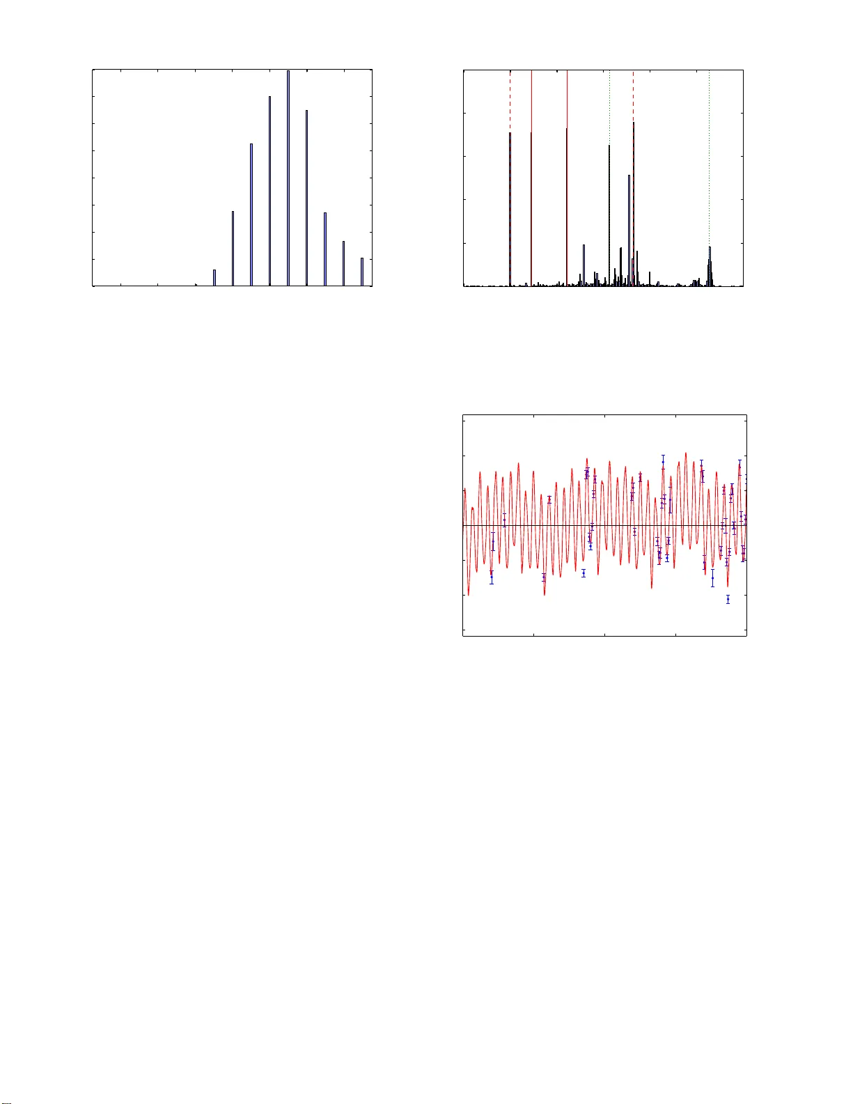
Mon. Not. R. Astron. So c. 000 , 000–000 (0000) Printed 15 August 2018 (MN L A T E X st yle file v2.2) F ast Ba y esian Inference for Exoplanet Disco v ery in Radial V elo cit y Data Brendon J. Brewer 1 ⋆ , Court ney P . Donov an 1 1 Dep artment of Statistics, The Univ ersity of Auckland, Private Bag 92019, Auckland 1142, New Ze aland T o be s ubmitted to MNRAS ABSTRACT Inferring the nu mber of planets N in an exoplanetar y system fro m radial v elo city (R V) data is a challenging task. Recently , it has b eco me clear that R V data can con- tain p erio dic signa ls due to s tellar activity , which can b e difficult to dis tinguish from planetary sig nals. How ever, even doing the infere nc e under a given s et of simplifying assumptions (e.g. no stella r activity) can b e difficult. It is co mmo n for the p oste- rior distr ibution for the planet parameters , such as o rbital pe r io ds, to b e m ultimoda l and to have other awkw ard features. In addition, when N is unknown, the ma r ginal likelihoo d (or evidenc e ) as a function o f N is required. Rather than doing separ ate runs with different trial v alues of N , we propo se an alternative approach using a trans-dimensiona l Markov Chain Monte Ca rlo method within Nested Sampling. The po sterior distribution for N can b e obtained with a single run. W e apply the metho d to ν Oph a nd Gliese 581, finding mo derate e vidence for a dditional signa ls in ν Oph with p e r io ds of 3 6.11 ± 0.03 4 days, 75.58 ± 0.8 0 days, and 170 9 ± 183 days; the po sterior probability tha t a t least o ne of these exists is 85 %. The results also s ug gest Gliese 581 hosts many (7-15) “planets” (or o ther causes of o ther p erio dic sig nals), but only 4-6 hav e well determined p erio ds . The analy s is of b oth of these da tasets shows phase tr ansitions exist w hich are difficult to negotia te without Nested Sampling. Key w ords: stars: plane ta ry systems — techniques: radial velocities — metho ds: data a nalysis — metho ds: s tatistical 1 INTRO DUCTION The number of known extrasolar planets has exploded in the l ast t w o decades. This has b een driven b y improv emen ts in all of the different techniques used to d etect and charac- terise exoplanets, including the radial velocity (R V) metho d (e.g. Sato et al. 2012), the transit method (e.g. Batalha 2014), and gravitational micro lensing (e.g. Benn ett et al. 2014; Y ee et al. 2014). The problem of inferring the properties of an ex o- planetary system from observ ational data can b e challeng- ing. In the case of radial velocit y d ata, the exp ected sig- nal due to an exop lanet is p erio dic, and the goal is to infer the number of planets in the system, as w ell as their prop erties suc h as orbital p eriods and eccentricities. Man y differen t techniques have been prop osed for doing this. These tec hniques fall in to tw o main classes: i) those based on p eriodograms (e.g. Zechmeis ter & K ¨ urster 2009), and ii) th ose b ased on mo del fitting in the Bay esian in fer- ence framewo rk, to d escribe the un certain ties probabilisti- ⋆ b j . brewe r@auckland .ac.nz cally (e.g. Gregory 2011; F eroz & Hobson 2014; T uomi 2011; Hou, Go o dman, & Hogg 2014). Bay esian mod el fitting via Mark ov Chain Monte Carlo (MCMC ) tends to be compu- tationally intensiv e, especially if w e wa nt to calculate the p osterior distribution for N , the number of p lanets. It is well kno wn th at R V datasets can contai n p eri- odic signals resulting from stellar activity rather than plan- ets, which can affect the conclusions w e dra w ab out exo- planet systems (e.g. Qu eloz et al. 2001; Bonfils et al. 2007 ; Rob ertson et al. 2014) . Therefore, it is imp ortant to develop mod els which attempt to d istinguish stellar activity signals from K ep lerian planet signals based on the sh ap e of the os- cillations and/or add itional data constraining the p erio ds of any stellar activity signals. W e do not ad d ress t h is im- p ortant challenge in the present pap er. Rather, we consider the p roblem of inferring the number N of Keplerian signals in an R V dataset in a computationally efficien t w a y , und er the simplifying assumption t hat only Keplerian signals are present in the data. W e in trodu ce a trans-d imen sional birth-death MCMC approac h (Steph ens 2000) to inferring N . When N is treated as just another mo del parameter, w e can obtain its p oste- c  0000 RAS 2 Br ewer an d Donovan rior distribution in a single run . In addition, rather than trying to sample the posterior distribution, we use Diffu - sive Nested Sampling (DNS Brewe r, P´ arta y , & Cs´ anyi 2011) whic h replaces the p osteri or distribution with an alterna- tive mixtur e of c onstr ai ne d priors , allo wing mixin g b etw een separated mo des. A s a result, we are able to sample t h e p osterior d istribution for N , and eval uate the marginal like- lihoo d (inclu d ing the sum o ver N ) in a single run whic h takes ab out 10 minutes on a 2-3 planet system. On th e other hand the approach of Gregory (2011) takes approx- imately 30 minutes p er planet (Gregory , priv. comm.). A C++ implementation of our meth o d is av ailable online at https://gi thub.com/e ggplantbren/Exoplanet under the terms of th e GNU General Public Licence. 2 INFERENCE Ba yes ian inference is the use of probability the- ory to describ e uncertainty (Sivia & Sk illing 2006; O’Hagan and F orster 2004). In this framew ork, we ap- proac h data analysis problems by first constructing a hyp othesis sp ac e , whic h is th e set of p ossible answ ers to the p roblem we are considering. Normally , this is the set of p ossible v alues of a vector of parameters θ whose val ues w e wan t to know. W e then assign probabilit y distributions called th e prior and the sampli ng distribution . The prior distribution p ( θ ) describ es our initial uncertain ty ab out whic h v alues of the parameters θ are plausible, an d the sam- pling distribution p ( D | θ ) describ es our initial uncertaint y abou t the d ata set we’ re going to observe, as a function of the u nknown parameters θ . When the data is k now n, our state of k n ow ledge about the parameter is up dated from the p rior p ( θ ) to th e p osterior distribution given by Bay es’ rule: p ( θ | D ) = p ( θ ) p ( D | θ ) p ( D ) (1) where p ( D | θ ) as a function of θ is called the lik elihoo d, once the actual dataset has b een sub stituted in. N ote that some authors do not distinguish b etw een a sampling distribution and a likelihoo d. Throughout this p ap er w e use th e term sampling distribut ion for p ( D | θ ) if we are discussing a prob- abilit y distribu t ion (actually a family of th em, indexed by θ ) o ver the set of p oss ible datasets. W e use the term likeliho o d when the actu al dataset has b een plugged in, when p ( D | θ ) b ecomes a scalar function (n ot a probability distribution) o ver the parameter space. The denominator, often called the evidenc e or mar ginal likeliho o d , is given by the expected v alue of th e likelihoo d with respect to the prior: Z = p ( D ) = Z p ( θ ) p ( D | θ ) d n θ (2) where the integral is ov er the entire n -dimensional parameter space. In the context of Bay esian computation, the prior is often denoted π ( θ ), the lik elihoo d L ( θ ), and the marginal lik elihoo d Z . 2.1 Infe rring the num ber of plane ts The number of orbiting planets, N , is an imp ortant param- eter. T o calculate the p osterior distribution for N , most au- thors consider v arious trial v alues of N , and calculate th e marginal like lihoo d p ( D | N ) = Z p ( θ | N ) p ( D | θ , N ) d n θ (3) for e ac h possible v alue of N (e.g. Gregory 2011; F eroz, Balan, & H obson 2011; F eroz & Hobson 2014 ; Hou, Go o dman, & Hogg 2014 ) , marginalising ov er all other mod el parameters. The posterior distribution for N can then b e found straightforw ardly by u sing Bay es’ rule with N as t h e only unknown parameter: p ( N | D ) = p ( N ) p ( D | N ) P N p ( N ) p ( D | N ) . (4) P opular method s for calculating the marginal likel ihoo d are Nested Sampling (Skilling 2006) and ideas related to ther- mod y namic integrati on (e.g. Neal 2001). Relationships be- tw een these methods are discussed by Cameron & Pettitt (2014) and P olson & Scott (2014). This traditional approach can b e very time consum- ing. Metho ds for calculating the marginal likelihoo d are al- ready more intensive than standard MCMC metho ds for sampling the posterior, b ecause they usually involv e a se- quence of probabilit y distributions (e.g. the constrained pri- ors in Nested Sampling, or the annealed distributions in thermo d ynamic in tegration) rather than a single distribu- tion (the p osterior). This intensive pro cess needs t o b e run many times, for N = 0, N = 1, N = 2, and so on. The traditional approach to inferring N also contradicts fundamental ideas in Bay esian computation. Imagine we are trying to compu t e the p osterior distribution for a parameter a in the presence of a nuisance parameter b . This is usually solv ed by exploring the join t p osterior for a and b , and then only lo oking at the generated v alues of a . Nob od y would suggest the wasteful alternative of using a discrete grid of p ossible a v alues and doing an entire N ested Sampling run for eac h, to get the marginal like lihoo d as a function of a . When the hyp othesis space for a is d iscrete, MCMC is still p ossible and there is no reason to switch to t h e w asteful alternativ e. 2.2 T rans-dimensi onal MCMC T rans-d imensional MCMC metho ds such as birth-death MCMC (Stephens 2000) or the more general revers ible jump MCMC (Green 1995) treat th e mo del d imension N as just another model p arameter. At fixed N , stan- dard techniques such as th e Metrop olis algorithm can b e used to explore the p osterior distribution. Add i- tional mo ves th at prop ose to change the v alue of N are also defined . The simplest of these are birth-death mo ves. More complicated mov es, suc h as split-and-merge, are p ossible but not alw a ys n ecessary . T rans-dimensional MCMC is a natural tool fo r a wide ran ge of astronom- ical data analysis problems (e.g. Umst¨ atter et al. 2005 ; W almswell et al. 2013; Brew er, F oreman-Mac key , & Hogg 2013; Jones, Kashy ap, & v an Dy k 2014) . In the exoplanet context, a birth mov e prop oses to add one more p lanet to the mo del. The new planet’s prop erties (p eriod, amplitude, eccentricit y , etc) are drawn from their prior distribution which may dep end on other other mod el parameters or hyp erparameters. The corresp onding d eath c  0000 RAS, MNRAS 000 , 000–000 3 mo ve simply c ho oses a planet curren tly in the model, and remo ves it. The acceptance probability for th ese mo ves is 1 if we w ant t o ex p lore the prior. T o imp lemen t th ese mov es in Nested Sampling (Skilling 2006), where the t arget d istribu- tion is p rop ortional to the prior but with a hard likel iho o d constrain t, then the acceptance probabilit y is 1 if t he pro- p osed mo ve satisfies the likel ihoo d constraint, and 0 if it does n ot. A recent pap er (Brew er 2014) in t rodu ced a general approac h to implementing trans-dimensional mo dels within Diffusive Nested S ampling (Brewer, P´ arta y , & Cs´ anyi 2011), a general MCMC algorithm. The Brew er (2014) soft w are predefines the Metrop olis prop osals for exploring trans-dimensional target d istributions, including when t he prior for the p rop erties of each mo del comp onent (i.e. each planet) is defined hierarc hically . 2.3 Phase transitions It is well kn o wn that Bay esian computation (using MCMC for example) can b e difficult when the p osterior distribution is multimodal or has strong d ep endencies b etw een param- eters. An u ncommon but less well-kno wn difficulty is the existence of phase tr ansitions (Skilling 2006). Imagine a high-dimensional un imo dal posterior distri- bution that is comp osed of a broad, h igh v olume but low density “slab” with a narro w, low volume but high density “spike ” on top of it. An example is a mixtu re of tw o concen- tric h igh-dimensional gaussians with d ifferent widths. If you ran MCMC on such a p osteri or, it would b e difficult to jump b etw een th e slab and the spike comp onents. If the MCMC is currently in the spike region (or phase) it will b e unable to escap e: a proposed mo ve into the slab will be rejected b ecause of the ratio of densities. Conv ersely , if the MCMC w as in the slab region, it would b e unlikely to go into the spike region, b ecause its volume is so small: it wo uld b e very unlikely to pr op ose to mov e into the spike. Thus, the situa- tion b eha v es much like a multimodal p osterior, despite on ly b eing unimo dal. If the slab contains a very small amoun t of p osterior probabilit y , it is not a problem if an MC MC algorithm sp en ds all its time in the spike. How ev er, this situation could still cause problems with the calculation of the marginal like- lihoo d if an n ealing metho ds are used. The thermo dynamic integ ral form ula gives the log of th e marginal lik elihoo d Z as an a verag e of log likel ihoo ds: log( Z ) = Z 1 0 h log [ L ( θ )] i β dβ (5) where the expectation is taken with resp ect to the dis- tribution wi th “in vers e temperature” β , prop ortional to π ( θ ) L ( θ ) β . Even if the slab con tains virtually zero proba- bilit y when β = 1 (i.e. the p osterior), for some v alues of the inv erse temp erature β the slab and the spike will b oth b e important. At these temp eratures the MCMC will fail to mix (it will incorrectly sp end all its time in either the slab or the spike, rath er t han mixing b etw een the tw o) and will give a misleading estimate of the av erage log likelihoo d at that temp erature and t h erefore an incorrect marginal likelihood estimate. Phase t ransitions are well kn o wn in statistical mechan- ics, but can also occu r in Ba yesi an data analysis. Typ- ically this occors when the data contains a “big” effect whic h p ro vides a lot of information ab out some parame- ters, and a “small” su b tle eff ect as w ell. Nested S ampling, and va rian ts suc h as DNS, are not affected by phase tran- sitions because the exploratio n only makes use of lik eli- hoo d r ankings , rather th an likeli ho od v alues themselves, and are th erefore inv ariant under monotonic transformations of the likelihoo d function. Pa rt of their output, the relation- ship b etw een th e likelihoo d L and the en closed prior mass X ( L ) = R π ( θ ) 1 [ L ( θ ) > L ] d n θ can b e used to diagnose whether the problem contains a p hase t ransition. In p ar- ticular, if th e graph of log( L ) v s. log ( X ) is conv ex at some p oint, then a phase transition exists (Skilling 2006). 2.4 Parameters and Priors T o fit a planet model to R V data, w e need parameters to describe the p rop erties of each planet. F or simplicit y , we de- scribe eac h planet by five parameters: the orbital p erio d P i , the semi-amplitud e (in metres p er second) of the R V signal A i , th e phase of th e signal φ i (defined such t h at φ = 0 gives an R V signal whose maximum is at t = 0), the eccentricit y e i , and the “viewing angle” ω i (also known as the longitude of the line of sigh t). W e defin ed our parameters su ch that in th e limit of zero eccen tricit y , the R V signal of a planet reduces to A i cos (2 πt/P i + φ i ). The unknown parameters are: n N , α , { ψ } N i =1 , m 0 , σ extra , ν o (6) where N is th e n umber of planets, α = { µ P , σ P , µ A } are hyperparameters hyp erparameters used t o define the prior for the p rop erties of t h e planets, and ψ i = { P i , A i , e i , φ i , ω i } are th e prop erties of p lanet i . The parameter m 0 describes a DC offset in the data, and σ extra and ν are parameters of the noise distribution whic h are discussed further b elo w. Note th at our p arameter ω i is stand ard, how ever φ i is n on- standard b ecause w e assert that φ i = 0 alw a ys implies the signal is at its maxim um at t = 0. Our parameter space is equiv alen t to the standard on e, w e are just u sing a different coordinate system. A stand ard assumpt ion for th e probability distribution of the data given t he parameters (known as the sampling distribution, which b ecomes the likelihoo d fun ction when the d ataset is known) is a normal distribution with standard deviation σ i known from the error bars in the data set. How - ever, it is u sually recommended to put in “safet y features”, in case the data set contains any discrepant measurements, or in case the error bars in the data set are und erestimated. T o ac hieve this, we used a student- t distribution instead of a n ormal distribution, with scale parameter p σ 2 i + σ 2 extra and shap e p arameter ν . The p arameter σ extra is an “ext ra noise” parameter that effectively in creases the size of th e er- ror bars, and the shap e p arameter ν allow s for heavier tails than a normal distribution. If ν is large, the student- t dis- tribution is app ro ximately a normal distribution, and if ν is small the noise distribution has muc h h ea vier tails. F or instance, when ν = 1 the stud ent- t d istribu t ion b ecomes a Cauc hy distribution. All of t he mo del assumptions are sp ecified in detail in T able 1. W e assigned hierarc hical p riors to some of the planet’s parameters (i.e. the prior for the p lanets’ parame- c  0000 RAS, MNRAS 000 , 000–000 4 Br ewer an d Donovan ters is defined conditional on some hyp erparameters). This allo ws th e mo del t o captu re the idea th at knowing the val - ues of some p lanet’s parameters provides some information abou t the parameters of another planet. Not using hierar- chica l priors u su ally implies a strong prior commitment t o the hyp othesis that the prop erties of the planets are spread out across th e whole domain of p ossible v alues, which is not necessarily the case. Most of our priors we re chosen to represent v ague prior knowl edge, rather than the judgement of an informed ex- p ert on extrasolar planets. Uniform distributions were used for p arameters such as phases, where time-translation sy m- metry seems plausible. F or some parameters we assigned th e distribution in terms of th e log of the p arameter, rather than the parameter itself, when the parameter is p ositive and un- certain by orders of magnitude. T ru ncated Cauch y d istribu - tions were used when there is a preferred v alue, but since these ha ve very heavy tails, the assumption is qu ite fail safe relativ e to other p ossible “informativ e” assignments suc h as normal d istribu tions. F or example, t h e prior for µ P , the typ- ical orb ital p erio d, is centered around 1 year b u t could b e as low as ≈ e − 21 years or as high as ≈ e 21 years , a very generous range. A uniform distribution for log( µ P ) wo uld hav e b een more conv enti onal, whereas the Cauch y distribu- tion expresses a slight preference for µ P b eing of order one year. An apparen tly strange c hoice is the conditional prior for the (logarithms of ) the orbital p eriods, which is a biex - p onential distribution given a lo cation parameter µ P and a scale parameter w P whic h d et ermines the width of the dis- tribution 1 . Rath er than assigning indep en dent priors t o the log p eriod s, the hierarchical mo del allow s for the p erio ds to “cluster around” a typical p eriod µ P if there is evidence for this. On the oth er hand, indep endent priors for the p erio ds w ould imply a strong prior commitment to the hyp othesis that the p erio ds are spread out across the whole prior vol- ume (equiv alen t to assuming a fi xed large v alue for w P ). A more conve ntional choi ce for the conditional prior giv en µ P and w P w ould hav e b een a normal distribution. How ever, the Brew er (2014) soft w are need s to know th e corresponding cumulativ e d istribution and its inv erse, which are not a v ail- able in closed form for the normal distribut ion. O u r prior for w P , which controls the diversit y of the log-p eriods, was uniform betw een 0.1 and 3, since it is un likel y t hat many planets hav e extremely similar or ex tremely different (o ver sever al orders of magnitude) orbital p eriod s. F or the velocity semi-amplitudes { A i } , we chos e an ex- p onential distribution given t h e hyperparameter µ A whic h sets the mean of the exp onential distribution. Ou r p rior for µ A spans many orders of magnitud e but expresses a slight preference for µ A b eing of order unity , using a Cauch y dis- tribution. The prior for the semi-amplitudes will influence how many of these low amplitude planets will b e inferred: if w e b elieve there are many , and t he data are u ninformativ e abou t low amplitude planets, then t he p osterior distribution for N will also indicate that there ma y b e many low ampli- tude planets. H ow ever, their other p rop erties, such as their 1 A biexp onen tial distribution with lo cation parameter µ and scale parameter w has probability density function p ( x | µ, w ) = 1 2 w exp  − | x − µ | w  . orbital p erio ds, will not b e well determined. The Beta prior for eccentricit y was su ggested by Gregory ( priv. comm) and is an approximatio n t o the inferred frequen cy distribution of eccentricities in the p opulation (Kipping 2013). 3 ORBIT LOOK-UP T ABLE The exp ected (noise-free) signal du e to an exoplanet is p eri- odic, bu t n on-sinusoidal when the orbit is not p erfectly cir- cular. The exp ected shap e m ( t ) of the v ariations is needed in order to ev aluate the likelihood function for any prop osed setting of the parameters. T o sav e time, w e pre-computed the prop erties of orbits as a function of eccentricit y . W e also made the standard assumption that the planets d o n ot in- teract, so the exp ected signal due to seve ral planets is t h e sum of the con tributions of eac h planet. Consider a test particle mo ving in t he x - y p lane under the influence of a p oin t mass at the origin. The motion of the test particle represents the reflex motion of the h ost star orbiting around th e center of mass of th e system. The equations of motion for the particle are: d 2 x dt 2 = − x r 3 (7) d 2 y dt 2 = − y r 3 (8) (9) where r = p x 2 + y 2 . The solutions to this system of equa- tions are elliptical orbits with th e fo cus at the origin. W e set the in itial position to (1 , 0), and the initial velocity to (0 , v ) where v ∈ [0 . 4 , 1]. If v = 1, the orbit is circular and as v decreases the orbit b ecomes more elliptical. F or trial v alues of v ranging from 0.4 to 1 in steps of 0.005, w e calculated the orbit, and sa ved the velocities dx dt and dy dt as a function of time to d isk. These sa ved orbits were used as a lookup table for constru cting the ex p ected sig- nal y ( t ) due to a single planet. Because of the initial con- ditions, the sim ulated orbits were all horizon tally aligned. If the observer is located on the x -axis a large distance from the origi n, th ey will measure m ( t ) = ˙ x ( t ). How ever, if the observer is located at an angle ω with respect to the x -axis, then the radial velocity measured will in stead b e m ( t ) = cos( ω ) ˙ x ( t ) + s in( ω ) ˙ y ( t ). Since the our orien tation with resp ect to the orbits is u nknown, eac h planet req uires a “viewing angle” parameter ω also known as the longitude of the line of sight (O hta, T aruya, & S uto 2005). The eccentric- it y of the orbit, in terms of v , is e = 1 − v 2 . By precomputing a set of orbits b efore run ning the MCMC, we are able to do ∼ 15,000 lik elihoo d ev aluations p er second p er CPU core. 4 DEM ONSTRA TION ON SIMULA TED DA T A T o test our prop osed metho dology , w e generated a sim u- lated dataset for a system with N = 7 planets. The dataset w as “inspired by” the ν Oph dataset (S ection 5), and con- tains tw o large signals with p eriods of 530 and 3120 d ays, whose semi-amplitudes are 291 m s − 1 and 181 m s − 1 re- sp ectively . The other fi ve planets hav e muc h low er semi- amplitudes, ranging from 4-30 ms − 1 . The standard devia- tion for the n oise in the data was 5 m s − 1 , so some of these c  0000 RAS, MNRAS 000 , 000–000 5 Quan tit y Meaning Prior Hyperpar ameters N Number of planets Uniform( { 0 , 1 , ... , N max } ) µ P Median orbital per io d (y ears) log( µ P ) ∼ Cauch y(location = 5 . 9 , scale = 1) T ( − 15 . 3 , 27 . 1) w P Diversit y of orbi tal p erio ds w P ∼ Uniform(min = 0 . 1 , max = 3) µ A Mean amplitude (metres per second) log( µ A ) ∼ Cauch y(location = 0 , scale = 1) T ( − 21 . 2 , 21 . 2) Planet Parameters P i Orbital per i od log( P i ) ∼ Biexp onen tial(location = log( µ P ) , scale = w P ) A i Semi-amplitude of signal Exponential(mean = µ A ) φ i Phase of signal Uniform(min = 0 , max = 2 π ) e i Eccen tricit y of orbit Beta( α = 1 , β = 3 . 1) T (0 , 0 . 8) ω i Viewing angle Uniform(min = 0 , max = 2 π ) Other m 0 Constan t DC offset Uniform(min = m 0 , min , max = m 0 , max ) σ extra “Extra noise” parameter log( σ ) ∼ Cauc h y(location = 0 , scale = 1) T ( − 21 . 2 , 21 . 2) ν Shape parameter for t -distribution for noise log( ν ) ∼ Uniform(mi n = log(0 . 01) , max = log(1000)) Data Y i Radial v elocity measurement s Studen t- t  lo cation = m ( t i ) , scale = q σ 2 i + σ 2 extra , s hape = ν  T able 1. All of the prior distributions in our Bay esian model. The priors for the planet parameters are defined conditional on the v alues of the hyperparameters. Uniform priors were used for parameters like phases. F or parameters where a rough initial guess is p ossible, hea vy-tailed Cauch y distributions we re used so this inform ation could b e take n into accoun t in a non-dogmatic wa y . Tim e units are i n da ys and amplitude units are in metres p er second. The maximum num ber of planets, N max , was set to 10. The prior lim its for m 0 we re set to the mi nimum and maximum v alue in the dataset, which i s not strictly a v ali d strategy . Some of the distributions were truncated for nume rical reasons, the truncated i nterv als ar e sp ecified wi th the T ( a, b ) notation. 0 500 1000 1500 2000 2500 3000 3500 Time (days) − 600 − 400 − 200 0 200 400 600 Radial V elocity (m/s) Figure 1. A simulated dataset that “resembles” the ν Oph dataset, whi c h we used to test our m ethodology . The dominant signal is from tw o large planets with p erio ds per io ds of 530 and 3120 days and semi-amplitudes of 291 m s − 1 and 181 m s − 1 resp ectively . There are also five muc h smaller planets whi c h con- tribute small additional effects to the data. lo w-amplitude signals should b e detectable. The sim ulated data is shown in Figure 1, along with th e true radial velocit y curve m ( t ) that w as used to generate the data. W e ran our algorithm on the simulated dataset to ob- tain samples from the p osteri or distribution. W e obtained 520 posterior samples. The p osterior d istribution for N , th e num ber of planets, is shown in Figure 2. The true num b er of planets, 7, is not the most probable v alue, but it does hav e substantial p robabilit y . The p osterior distribution su ggests that N could b e anywhere from 6 to 10. The posterior distribution for the perio ds { P i } N i =1 is sho wn in Figure 3 . Because of the label switching degen- 0 2 4 6 8 10 Number of Planets 0 50 100 150 200 250 300 Number of Posterior Samples Figure 2. The p osterior distri bution for the num ber of planets N giv en the simulated dataset. The true num ber of planets was 7. eracy , the p osterior distribution for each p erio d is identical , so we p o oled the samples for all p eriod s. Defining t h e log- p eriods by S i = log 10 [ P i / (1 da y)], Figure 3 is a Monte Carlo representa tion of the mixture distribution f ( S ) = 10 X N =0 p ( N | D ) N X i =1 p ( S i | N , D ) . (10) If a certain p erio d is accurately measured (i.e. it ap p ears in close to 100% of t he p osterior samples and the distribution for its p eriod is very narrow) then it will app ear in Figure 3 with a height of ∼ 520. If the uncertaint y in the p erio d is larger th an the histogram bin width then the p eak will b e spread ov er several bins. The p osterior distribution for th e p erio ds, shown in Fig- c  0000 RAS, MNRAS 000 , 000–000 6 Br ewer an d Donovan 1 . 0 1 . 5 2 . 0 2 . 5 3 . 0 3 . 5 4 . 0 log 10 (Period/days) 0 100 200 300 400 500 600 Number of Posterior Samples Figure 3. The p osterior distribution for the p erio ds giv en the simulated data set. The solid lines are the true perio ds, s i x of which were detected wi th high p osterior probability . 1 . 0 1 . 5 2 . 0 2 . 5 3 . 0 3 . 5 4 . 0 − 1 . 0 − 0 . 5 0 . 0 0 . 5 1 . 0 1 . 5 2 . 0 2 . 5 3 . 0 log 10 [Amplitude (m/s)] 1 . 0 1 . 5 2 . 0 2 . 5 3 . 0 3 . 5 4 . 0 log 10 (Period/days) 0 . 0 0 . 1 0 . 2 0 . 3 0 . 4 0 . 5 0 . 6 0 . 7 Eccentricity Figure 4 . The joint p osterior distribution f or the p erio ds and the amplitudes (top panel) and the p erio ds and eccen tricities (b ottom panel) from the simulated dataset. The true v alues are plotted as circles. ure 3, shows th at six of t h e true p erio ds were reco vered, with probabilit y close to 1. One perio d (with log 10 P i ≈ 1 . 15) whic h w as actually present was not “detected” b ecause it had a very small amplitude. W e note that t h e p osterior p rob- abilit y near th is p erio d should not b e precisely zero. There is also some evidence for p erio ds whic h did not actually ex ist, how ever the p osterior probabilities for these p eaks are n ot close to 1. The joint p osterior distribution for th e p eriod s and the amplitudes of the signals is shown in Figure 4 along with t h e eccentri cities. As with Figure 3, th e samples for all planets w ere combined. The true va lues are also plotted as circles. Clearly , t h e reason the p eriod of log 10 ( P i ) ≈ 1 . 15 was not “detected” was that it had a very low amplitude of approx- imately 4 m s − 1 whic h is b elo w the noise level. 5 APPLICA TION TO ν OPH The ν Oph system is generally accepted to hav e tw o confirmed planets (e.g. Quirrenbac h, Reffert, & Bergmann 2011; S ato et al. 2012; H ou, Goo dman, & Hogg 2014), with 2 4 6 8 10 Number of Planets 0 50 100 150 200 250 300 350 Number of Posterior Samples Figure 5. The p osterior distri bution for the num ber of planets N orbiting ν Oph. The p osterior pr obabilit y of N > 2 is ab out 88%, ho w ev er the prior pr obabilit y of N > 2 was alr eady hi gh due to the uniform prior for N . p eriods of 530 . 3 and 3190 days. T o test our approach we applied it to th e R V data from Sato et al. (2012). The p os- terior d istribu tion for N , th e num ber of p lanets, is sho wn in Figure 5, show ing that N could b e an ywhere from 2 to 10, and t he p osterior p rob ab ility that N > 3 is ab out 88%. Of course, th ese extra p ossible signals are n ot necessarily a planet but a feature in the data which is bet t er explained by a p eriodic signal t han by n oise (and may hav e b een ex - plained by correlated noise, had we included it). The p osterior d istribution for the logarithms of the p e- riods is shown in Figure 6. As in Section 4, the p osterior samples for all p eriods w ere combined to make this figure, whic h shows several prominent p eaks. The tw o p eaks with vertica l dashed lines are the commonly accepted p eriods of 530 and 3190 days, and the other prominent p eaks (i.e. sig- nals which h a ve a moderate probabilit y of existence) ha ve p eriods of 36.11 ± 0.034 d a ys, 75.58 ± 0.80 days, and 1709 ± 183 days. As with an y MCMC output, if w e are inter- ested in the probabilit y of any prop osition Q (for example, “ Q ≡ a p lanet ex ists with p erio d b etw een 35 and 37 days”), w e can calculate th e p rop ortion of the p osterior samples for whic h Q is true, which (if we ha ve a lot of samples) is a Mon te Carlo estimate of t h e p osterior probability of Q . F or ν Oph, we calculated the p robabilit y that at least one of these “extra” signals (beyond the tw o commonly accepted ones) exists, as 85%. Given that they exist, th eir amp litud es are low, around 5-40 metres per second, whic h w e note is above the noise level. A n example mo del fit to the data is sho wn in Figure 7. Figure 8 shows the relationship b etw een the lik elihoo d L and th e enclosed prior mass X for the ν Oph analysis. These plots are a standard outp ut of Nested Sampling anal- yses, and p rovide insights into t h e structure of the problem. Conca ve-up regions of t his curve indicate p hase t ransitions whic h can cause severe p roblems for annealing-based meth- ods, and sometimes even for sampling the p osterior d istribu- tion. I n this analysis, the mo dels with a third signal exist to the left of the phase transition at log( X ) ≈ − 70, and mo dels without the signal exist to the right of the ph ase transition. c  0000 RAS, MNRAS 000 , 000–000 7 1 . 0 1 . 5 2 . 0 2 . 5 3 . 0 3 . 5 4 . 0 log 10 [Period (days)] 0 500 1000 1500 2000 Number of Posterior Samples Figure 6. The p osterior distribution f or the orbital p erio ds in the ν O ph system. The tw o dashed vertical li nes are the com- monly accepte d p eri ods of 530 . 3 and 3190 days. The next most prominent p eaks with w ell determined p erio ds are at log p erio ds of around 1.6, 2.4, and 3.3, corresp onding to p eri ods of 36.11 ± 0.034 da ys, 75.58 ± 0.80 days, and 1709 ± 183 day s. 0 500 1000 1500 2000 2500 3000 3500 Time (days) − 600 − 400 − 200 0 200 400 600 Radial V e locity (m/s) Figure 7. The ν Oph r adial velocity data and an example mo del fit which i ncludes a third p erio d. The amplitude of this additional signal is low but is ab out t wice the reported errorbars on the measuremen ts. Mixing b etw een th ese tw o phases is crucial for accurately computing th e p osterior probability that extra signals ex ist. The m arginal likelihoo d for our model was log( Z ) ≈ − 220 . 5. Nested Sampling also allows for calculation of the “information”, or Kullback-Leibler divergence (a quantit y in information theory) from the prior to the p osterior, whic h quantifies how muc h we learned ab out the p arameters: H = Z p ( θ | D ) log  p ( θ | D ) p ( θ )  dθ (11) An intuitive interpretation of this quantit y is th e num b er of times t h e prior distribut ion had t o b e compressed by a factor of e (if the logarithm in the form ula is a natural logarithm) − 120 − 100 − 80 − 60 − 40 − 20 0 log( X ) (nats) − 500 − 450 − 400 − 350 − 300 − 250 − 200 − 150 − 100 log( L ) Figure 8. Log li k eliho od vs. enclosed prior mass (a standard output of Nested Sampling al gorithms) f or the ν Oph analysis. There are several phase transitions (concav e-up regions) present. The small one at log ( X ) ≈ − 70 separates mo dels which contain additional si gnals from mo dels that do not. Without using Nested Sampling it w ould be more difficult to mix betw een these t wo situations and calculate the p osterior pr obability for the existence of the additional signals. to get to th e p osterior distribution. F or the ν O ph data the information w as H ≈ 76 . 6 nats (natu ral u n its) or 111 bits, so the p osterio r o ccupies ab out e − 76 . 6 times the p rior volume. 6 APPLICA TION T O GLIESE 581 The red dwarf star Gliese 581 is thought to h ost several p lan- ets. Exactly how many is a matter of considerable debate. According to Rob ertson et al. (2014), there are tw o plan- ets (b and c, with p erio ds 5.36 and 12.91 days resp ectively) whose existence is generally accepted, tw o more (d and e, with p eriods 66 and 3.15 d a ys resp ectively) whose existence w as mostly accepted, and another tw o (f and g, with p eriod s 433 and 36.5 d ays resp ectivel y) whose existence wa s gener- ally doubted. How ev er, Rob ertson et al. (2014) found th at planets d and g do not exist but are signals due to stellar activit y . While our model cannot accoun t for stellar v ari- abilit y and contribute to that particular discussion, it is a chal lenging and interesting dataset from an inference p oint of v iew. T o run our co de on the combined dataset from the HARPS and HIRES sp ectrographs, we extended the mo del to include separate DC offsets for each instrument, as wel l as separate “extra noise” parameters s 0 and ν . W e also in- creased N max from 10 to 15 for th is system. The p osterior d istribution for N is shown in Figure 9, and shows strong evidence for at least eigh t p eriod s ( P ( N 6 7 | D ) = 0 . 012). Some authors (e.g. T uomi 2011) recommend that th e probabilit y of N planets should b e > 15 0 times greater th an the probability of N − 1 planets existing b e- fore making a claim that N planets have b een definitively detected. Such a decision rule is presumably equiv alent to a utility function where false p ositives are muc h wors e than false negatives. W e n ote that app lying this ru le to our re- sults, we would assert N = 6, even though th is h as a very small p osterior probability . c  0000 RAS, MNRAS 000 , 000–000 8 Br ewer an d Donovan 2 4 6 8 10 12 14 Number of Planets 0 20 40 60 80 100 120 140 160 Number of Posterior Samples Figure 9. The posterior distri bution for the n umber of planets N orbiting Gliese 581. It is now recognised th at there are many p ossible sources for oscillations in a data set and not all such os- cillations should b e claimed as planets. Our mo del cannot distinguish betw een oscill ations due to planets and oscilla- tions due to stellar activit y: any oscillations found in the dataset will b e describ ed as “planets” by the mod el. An- other important consideration is t h e physical stabilit y of the orbital system which is ignored by t h is type of analysis (T´ oth & Nagy 2014 ). How ever it is interesting that we fin d many more signals in the d ata t h an previous authors. By insp ecting t he p osterior distribution for the p erio ds (Fig- ure 10), we see that only 4 of the p erio ds are w ell deter- mined and hav e a p osterior probability close t o 1 (i.e. they are present in all samples), correspond ing to th e known p e- riods of Gliese 581 b, c, d, and e. The oth er “p erio ds” are more uncertain. As with ν Op h, w e can calculate the p oste- rior probability of any hypothesis ab out Gliese 581 by com- puting t he fraction of t h e p osterior samples that h a ve that prop erty . The p osterior probabilities for planets b, c, d, and e, are close to 1. The p osterior p robabilit y a signal exists with log 10 ( P ) ∈ [1 . 55 , 1 . 57] is 88%, and the probab ility for a signal with log 10 ( P ) ∈ [2 . 6 , 2 . 8] is 85%. One p ossible explanation for the large n umber of in- ferred signals that a non- sinusoi dal signal d ue to stellar activit y is b eing mo delled as severa l p erio ds (e.g. as hap- p ens in asteroseismology when sinusoidal mo dels are used; Brew er et al. 2007 ), and if the model were extended to in- clude a “sto chastic” oscillation ( e.g. Brewer & St ello 2009), the number of perio ds detected ma y b e reduced su bstan- tially . Another contributing factor is the prior for the ampli- tudes. With these kind s of mo dels, t h e p osterior distribu tion for N can b e influ enced by th e prior for the amplitudes A i . Man y authors assig n indep endent b road priors t o t he am- plitudes, and this causes the “Occam’s razor” p enalt y for adding extra signals to b e qu ite strong. Since w e u se a hi- erarc hical prior for the amplitudes, if some amp litud es are found to b e lo w, µ A will b ecome small. When µ A is small, it is like ly th at any extra signals will hav e small amplitudes, so t he “Occam’s razor” effect is weak er. A n ex ample mod el fit for Gliese 581 is show n in Figure 11. The marginal like lihoo d w as log ( Z ) ≈ − 616 . 3 and the 0 . 0 0 . 5 1 . 0 1 . 5 2 . 0 2 . 5 3 . 0 log 10 [Period (days)] 0 200 400 600 800 1000 Number of Posterior Samples Figure 1 0. The p osterior distribution for the orbital per i ods in the Gliese 581 system. T he solid l i nes are Gliese 581 b and c, the dashed lines are “planets” d and e, and the dotted lines are f and g. 2700 2750 2800 2850 2900 Time (days) − 30 − 20 − 10 0 10 20 30 Radial V elo city (m/s) Figure 11. A p ortion of the Gliese 581 data and an example model fit. information was H ≈ 130 . 4 n ats. This compares fav ourably to the marginal likelihoo d of − 640 . 1 (for a 6-planet mod el) found by Hou, Go o dman, & H ogg (2014), although it is un- clear whether w e used exactly the same dataset. Interest- ingly , th e log-lik elihoo d curve (Figure 12) shows th is prob- lem h as tw o phase transitions. While these do not affect t h e p osterior d istribution (as they did for ν O ph), th ey w ould cause difficulties if w e tried to calculte the marginal likeli- hoo d using annealing. 7 CONCLUSIONS In t his pap er we introd uced a trans-d imensional MCMC ap- proac h to inferring the number of p lanets N in an exoplane- tary sy stem from radial vel ocity data. The MCMC was im- plemented using the framew ork of Brew er (2014) which de- fines trans-dimensional birth and death mo ves, and do es the c  0000 RAS, MNRAS 000 , 000–000 9 − 200 − 150 − 100 − 50 0 log( X ) (nats) − 1400 − 1200 − 1000 − 800 − 600 − 400 log( L ) Figure 1 2. Log l ikelihoo d vs. enclosed prior mass for the Gliese 581 analysis. The tw o concav e-up regions (at log( X ) ≈ − 25 and -45) corresp ond to phase transitions. Thermal approac hes to this problem would pr o duce misleading estimates of the mar ginal li ke - liho od b ecause they wou ld mi x p oorl y at temp eratures around 11 and 4. sampling with respect to a Nested Sampling target d istribu- tion, rather than directly sampling t h e posterior. This ap- proac h allo ws us to compute the results in a single ru n, which provides p osterior samples and an estimate of the marginal lik elihoo d. By using Diffusive N ested Sampling, instead of directly try in g to sample the p osterior distribution, we can o vercome difficult features in the problem, such as p h ase transitions and (to some extent) multiple mo des. W e applied the co d e to tw o well-studied R V datasets, ν Op h and Gliese 581. I n ν Oph , we found some evidence for additional signals with low amplitud e, but with severa l p ossible solutions for their p eriod s. Given our modelling as- sumptions, the posterior probability at least one of t hese additional signals is real is 85%. The p osterior distribution conta ins mo dels b oth with and without these additional sig- nals, how ever, these are separated by a p hase transition. Therefore mix ing b et w een th e tw o situations would b e in fre- quent if w e simply tried to sample th e p osterior distribution. With the com bined HIRES +HARPS dataset from Gliese 581, we found ev id ence for a large num ber of “plan- ets”, although only four h ave wel l determined p eriods, cor- respond ing to the Gliese 581 b, c, d, and e. Sin ce our mo del does n ot include any possibility of stellar v ariabilit y , any such p erio dic signals will b e attributed to “planets”. Includ - ing non-planetary stellar v ariabilit y is a crucial next step. ACKNO WLEDGEMENTS It is a p leasure to thank F eng ji Hou and David H ogg (NYU) for inspiring me (BJB) to finally wo rk o n this problem, and Phil Gregory (U BC) for writing so many interesting pap ers on it. W e al so thank T om Loredo (Cornell) and Dan F oreman-Mac key (NYU) for interesting con ve rsations and feedback, and Ben Montet (Caltec h) and Geraint Lewis (Sydney ) for helpful discussions. The referee also provided excellen t suggestions for improving the manuscript. This work was supp orted by a Marsden F ast Start grant from th e Roy al So ciety of New Zealand. REFERENCES Batalha N. M., 2014, PNAS, 111, 12647 Bennett D. P ., et al., 2014, Ap J, 785, 155 Bonfils, X., Ma yor, M., Delfosse, X ., et al. 2007, A&A , 474, 293 Brew er B. J., Stello D., 2009, MNRAS , 395, 2226 Brew er B. J., Bedding T. R., K jeldsen H ., Stello D ., 2007, ApJ, 654, 551 Brew er B. J., P´ artay L. B., Cs´ an yi G., 2011, St atistics and Computing, 21, 4, 649-656. arXiv:0912.238 0 Brew er B. J., F oreman-Mack ey D., Hogg D. W., 2013, AJ, 146, 7 Brew er, B. J., 2014, ArXiv: 1411.3921 Cameron E., Pettitt A., 2014, Statistical Science, V ol. 29, No. 3, 397-419 F eroz F., Hobson M. P ., 2014, MNRA S, 437, 3540 F eroz F., Balan S. T., Hobson M. P ., 2011, MNR A S, 415, 3462 Green, P . J., 1995, Reversible Jump Marko v Chain Monte Carlo Computation and Ba yesi an Mo del Determination, Biometrik a 82 (4): 711732. Gregory P . C., 2011, MNRAS, 415, 2523 Gregory P . C., 2011, MNRAS, 410, 94 Hou F., Goo dman J., Hogg D. W., 2014, arXiv, arXiv:1401.61 28 Jones D. E., Kashy ap V. L., v an Dy k D . A., 2014, arXiv, arXiv:1411.74 47 Kipping D. M., 2013, MNRAS, 434, L51 Neal, R. M., 2001, Statistics and Computing 11.2, 125-139. O’Hagan, A., F orster, J., 2004, Bay esian inference. London: Arnold. Ohta Y., T aruya A., S u to Y., 2005, ApJ, 622, 1118 P olson N. G., Scott J. G., 2014, arXiv, Queloz, D., Hen ry , G. W., Siv an, J. P ., et al. 2001, A&A, 379, 279 Quirrenbac h A., Reffert S., Bergmann C., 2011, AIPC, 1331, 102 Rob ertson P ., Mahadev an S., End l M., R o y A., 2014, Sci, 345, 440 Sato B., et al., 2012, P ASJ, 64, 135 Sivia, D. S., Skilling, J., 2006, Data A n alysis: A Bay esian T utorial, 2nd Edition, Oxford U niversit y Press Skilling, J., 2006, “N ested Sampling for General Bay esian Computation”, Ba yesia n Analysis 4, pp. 833-860 Stephens, M., 2000, “Ba yesia n analysis of mixture mo dels with an unkn own n umber of comp onents-an alternativ e to reversible jump method s.”, Annals of Statistics, 40-74. T´ oth Z., Nagy I., 2014, MNRA S, 442, 454 T uomi M., 2011, A& A, 528, L5 Umst¨ atter R., Christensen N., Hendry M., Meyer R ., Simha V., V eitch J., Vigeland S., W oan G., 2005, PhRvD, 72, 022001 W almswell J. J., Eldridge J. J., Brewer B. J., T out C. A., 2013, MN R AS, 435, 2171 Y ee J. C., et al., 2014, ApJ, 790, 14 Zec hmeister M., K ¨ urster M., 2009, A&A , 496, 577 c  0000 RAS, MNRAS 000 , 000–000