Defining a Trend for a Time Series Which Makes Use of the Intrinsic Time-Scale Decomposition

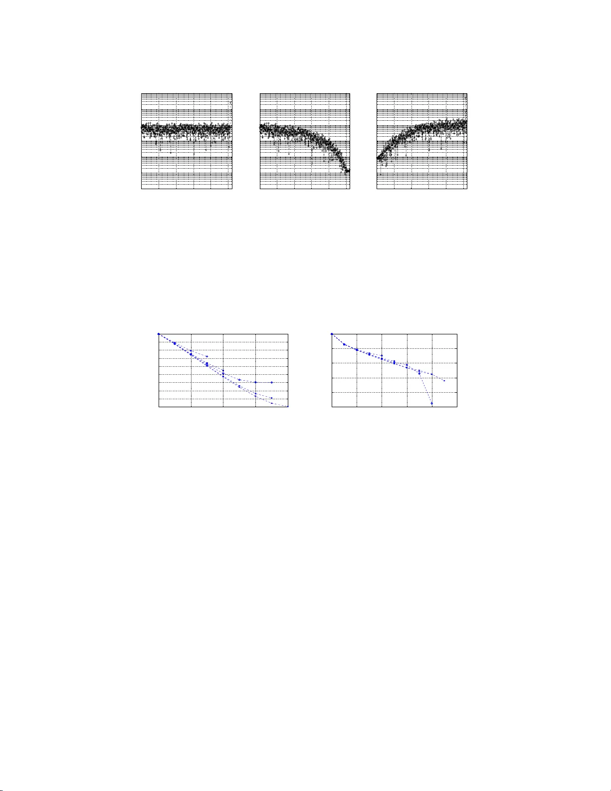
Defining a T rend for a Time S e ries Whic h Mak es Use of the Intrinsic T ime-Scale D e comp osition Juan M. Restrep o 1 , 2 , 3 , Shank a r V enk atarama ni 1 , 2 , Darin Comeau 2 & Hermann Flasc hk a 1 , 2 1 Mathematics Department, 2 Progr am of Applied Mathematics, 3 Physics Department, Univ ersity of Arizo na, T ucson AZ 8 5716 USA E-mail: restr epo@ma th.arizona.edu Abstract. W e prop ose criteria that define a tr e nd fo r time series with inhere nt multi- scale features. W e call this tr e nd the ten dency of a time ser ies. The tendency is defined empirically by a set o f criteria a nd ca ptur es the la rge-sca le temporal v aria bilit y of the original sig nal as well a s the most frequent even ts in its histogra m. Among other prop erties, the tendency has a v aria nce no larg er than that of the orig inal sig nal; the histogram of the difference b etw ee n the or iginal signal and the tendency is a s symmetric as p ossible; a nd with reduced co mplex it y , the tendency ca ptures essential features of the signal. T o find the tendency we first use the Intrinsic Time-Scale Decomp osition (ITD) of the signal, introduced in 2007 b y F r ei and Oso rio, to pro duce a set of ca ndidate tendencies. W e then a pply the cr iter ia to ea ch of the candidates to sing le out the o ne that be st agrees with them. While the criteria for the tendency are indep endent of the signal deco mpo s ition scheme, it is found that the ITD is a simple and stable methodology , well suited for m ulti-scale signals . The ITD is a relatively new decomp osition and little is known ab out its outcomes. In this study we take t he first steps tow a rds a probabilistic model of the ITD analysis of ra ndom time se r ies. This analys is yields details concerning the universalit y and scaling prop er ties of the comp onents of the decomp ositio n. AMS c lassification scheme n umbers: 62M0 9,62M10 ,62M20,6 2G05,62G08 Keywor ds : tendency , trend, non-statio na ry , non-parametrtic, m ulti-scale, in trinsic time- scale dec omp osition, time serie s, empirical model decomposition Submitted to: New J. Phys. 1. In tro duction Finding the trend of a time s eries is a fundamen tal analytical task. T o v arying degrees, the definition of t he term “trend” is dep enden t on the metho dolo g y used to compute it. Some trending strategies are optimal and thus v ery attr a ctiv e b ecause the optimalit y Ru nning title: The Time Series T endency 2 criteria provide mathematical constraints with whic h to in terpret the time series trend. Not all optimal trends deliv er us eful trends. A n example of a non-optimal trend is the Ho drick-Pres cott Filter (see (Ho dric k & Prescott 1997)) , which is widely used in econometrics. This pap er prop oses a new empirically-defined trend for an inheren tly m ulti-scale, finite time series. In an econometric con text, the trend is often used to capture the long er time scale structure of the mar kets, by filtering o ut high frequency ev ents that migh t b e more relev an t to shorter time scale c hanges. It is used this w ay in the ph ysical sciences a s w ell. Our in terest in this to pic was motiv ated by the problem of trend determination in a geoscience con text, where, in addition t o the remov al o f biases, one is often confronted with the necessit y of analysing signa ls with the aim o f reco v ering structural asp ects of the signal that can b e captured o r explained b y ph ysical mo dels. Geoscience problems often inv olv e m ulti-ph ysics and other sources of complexit y whic h manifest themselv es in a time series with a rich v a riet y of time scales. There is no rig orous definition of “m ulti-scale” signals, but in the phy sical mo deling commun ity the adjectiv e is applied to signals that are the result of the coupling of inheren t degrees of freedom (sometimes giv en b y sp ectral comp onen ts). F urthermore, it is frequen t ly the case in geoscience that the time series to b e analysed is short, of length muc h shorter than the n umber of degrees of freedom of the sys tem that generated the series; sometimes to o short to b e a menable to law-of-large n um b ers statistics. The pro cedure w e pro p ose to find the tendency is a tw o-stage pro cess: w e first decomp ose the signal in a series o f time series o f progressiv ely low er complexit y , and then w e apply a set o f criteria to these and single out the decomp osition mo de that b est satisfies the criteria. This mo de is declared to b e the tendency of the signal. While w e employ the In trinsic Time Decomp osition (ITD) of (F rei & Osorio 2007), the strategy could b e a pplied to other algorithms, suc h as the Emprical Mode Decomp osition (EMD), (Huang et al. 1998, W u & Huang 20 09, W u et al. 2007). In fact, a similar pro cedure has b een prop osed in connection with EMD (see (Moghtaderi et al. 2011, Mogh taderi et al. 2013 )): the EMD mo des a r e calculated, and a time series represen ting the t rend is built according to certain prescriptions. Most every thing that is know n to date ab out the ITD will b e review ed in Section 2; the algorithm that p erforms the decomp osition app ears in the App endix. In Section 2 w e summarize results of computer exp erimen ts on rando m signals tha t suggest certain probabilistic and scaling f eatures in the ITD decomp osition. In Section 3 w e initiate a mathematical analysis of these numerical results. This analysis migh t b e a pplicable to the EMD its v arian ts, suc h as those prop osed b y (Hou & Shi 20 11) and (Ob erlin et al. 2012). W e also use computer exp erimen t s to draw attention to the influence of b oundary conditions o n the o utcomes, fo cusing only on the ITD. Boundary effects are seldom highlighted in the EMD and ITD pap ers, but we find that for some signals, the b oundar y conditio ns can hav e a significan t effect on the outcomes a nd thus on t he construction of t he tendency from the comp onen ts of t he decomp osition. This discu ssion app ears in Section 4. Ru nning title: The Time Series T endency 3 Section 5 in tro duces the criteria that are us ed to pic k the ITD mo de that is de clared to b e the tendency . The criteria ar e empirically-based notions o f signal informat ion whose implemen tatio n is discussed in Section 6. In that section, w e illustrate the application of the tw o-step pro cess for finding the tendency on deterministic and random signals as w ell as on real geoph ysical signals. In the latter group, w e will feature an analysis o f the p ost-industrial temp erature record in Mosco w (a v ailable from (NASA/GISS 2013)). Ra hmstorf a nd Coumou (see (R ahmstorf & Coumou 2011)) set out to determine w hether the extrem e Mosco w summer tem p eratures of 2010 w ere outlier samples of climate or the result of a n ev er w arming Earth. Their analysis of extreme ev ents dep ends o n t he prop er determination of a sensible long-time trend, o r ”climate.” In Section 7 w e summarize the outcomes of the analysis and the o utcomes of the tendency calculations, and t a k e the opp ortunit y to compare, in general terms, the ITD tendency and the EMD trend. 2. The In trinsic Time-Scale Decomp osition The In tr insic Time-Scale Decomp osition (ITD) is a purely algorithmic, non-lossy iterativ e decomp osition of a time series { Y ( i ) } N i =1 . A t t he first stag e, the signal is decomp osed in to a pr op er r otation R 1 ( i ), an oscillating mo de in whic h maxima and minima are p ositive and negativ e, r espective ly , and a residual B 1 ( i ) called b aselin e . The baseline B 1 is no w decomp osed in the same fashion, pro ducing a proper rot a tion R 2 and a baseline B 2 , and so on. The pro cess stops when the resulting baseline has only t w o extrema, or is a constan t. If there are D steps a ltogether, the decomp o sition has the fo rm B 0 ( i ) := Y ( i ) = B D ( i ) + D X j =1 R j ( i ) , i = 1 , ..., N . (1) Rotations and baselines satisfy the relation B j ( i ) = B j +1 ( i ) + R j +1 ( i ) , i = 1 , ..., N ; j = 0 , ..., D . (2) P aren thetically , we note that in the algorit hm as describ ed in (F rei & Osorio 20 0 7) there is one, and o nly one, adjustable parameter denoted by α , whic h has b een set to α = 1 / 2 in ouer study . In general, the rota t ion signal at the j th lev el will b e ”noisier” than t he rotatio n signal at ( j + 1) th . The proper rotations are not orthogonal; moreov er, the de comp osition is not linear, in the sense tha t a decomp osition of the sum of time series is not equal to the sum of the decomp ositions of eac h of the signals. Let { τ j k } , k = 1 , 2 , .., K b e the times at which the extrema of B j ( i ) o ccur. (In the ev ent that there are sev eral succes siv e data p oints with the same extremal v alue, we tak e τ j k to corresp ond to the time of t he rightmost o f these extremal v alues). The ba seline B j +1 ( i ) is constructed by a piecewise linear formula: in the in terv al i ∈ ( τ j k , τ j k +1 ], Ru nning title: The Time Series T endency 4 b et w een successiv e extrema, B j +1 ( i ) = B j +1 k + ( B j +1 k +1 − B j +1 k ) ( B j k +1 − B j k ) ( B j ( i ) − B j k ) , (3) where the knots are B j k := B j ( τ k ). The formula that generates the knots is B j k +1 := B j ( τ k +1 ) = 1 2 " B j k − 1 + ( τ j k − τ j k − 1 ) ( τ j k +1 − τ j k − 1 ) ( B j k +1 − B j k − 1 ) # + 1 2 B j k . (4) The construction guarantees that the residual function R j +1 ( i ) = B j ( i ) − B j +1 ( i ) , i = 1 , 2 , ..., N , (5) is monotonic b et w een adja cen t extrema. F ig ures illustrating the construction ma y b e found in (F rei & Osorio 2007). One m ust also decide on a b oundary condition at the tw o ends. The effects of differen t c ho ices will b e discussed in Section 4 . W e shall inte rpret the end p oin ts as extrema, a nd tak e the corresp onding baseline knots to b e av erages of the first and last pair of extrema, B j 1 = B j (1), and B j K j = B j ( N ): B j +1 1 = 1 2 ( B j 2 + B j 1 ) and B j +1 K j = 1 2 ( B j K j − 1 + B K j ) . (6) These will b e called fr e e b oundary conditions. The decomp osition ends when j = D , whic h is when a prop er rot a tion cannot b e constructed from this last baseline. Baseline B D ( i ) will only hav e t w o knots: B D k =1 , 2 , the t w o end p oin ts. W e no w state a few imp ortan t prop erties of the ITD decomposition, largely follo wing (F rei & Osorio 200 7 ). (i) The baselines giv en in (3) can b e rewritten as a con vex com bination; viz. , B j +1 ( i ) = (1 − s j k ( i )) B j k + s j k ( i ) B j k +1 , s j k ( i ) = B j ( i ) − B j k B j k +1 − B j k , where s j k ( i ) ∈ [0 , 1], and j = 0 , 1 , .., D ; (ii) The knots, (3), at lev el j + 1 can also b e written as B j +1 k = 1 2 B j k + B j k + 1 2 τ j k +1 + τ j k − 1 − 2 τ j j τ j k +1 + τ j k − 1  B j k +1 − B j k − 1  , (7) where the ov erline indicates av erage of nearest neighbors; (iii) The ITD decomp osition is am big uo us with regard to ha ndling the end p oints of a finite time series, and thus, differen t end conditions can generate differen t ITD decomp ositions. See Section 4; (iv) The baseline extraction step can b e thought of as a nonlinear op erator L , homogeneous with resp ect to indep enden t rescaling of the abscissa and also the ordinate: B j +1 = L B j and R j +1 = (1 − L ) B j . (v) The B j and R j are monotonic b etw een successiv e extrema, since they are obtained, in succession, through linear transformations; Ru nning title: The Time Series T endency 5 (vi) It follows from t he ab o v e pro p ert y , that the ℓ 2 -norm o f B j is similar (to within a constan t) to the ℓ 2 -norm of a n approximation of the same signal, built b y connecting extrema with piece-wise linear segmen ts; (vii) The extrema of B j are inflection p oints or extrema of B j +1 ; (viii) Bet w een extrema of B j , B j +1 has the same smo othness a s B j ; (ix) At extrema of B j , B j +1 will b e contin uous and differentiable, but not alwa ys t wice differen tia ble; (x) R j +1 ( i ) will ha v e extrema at the same lo cations as B j ( i ). 2.1. R andom signals W e w ant to understand some basic features of the ITD b efore w e try to extract the tendency o f a realistic signal. Since w e use the ITD to strip r a ndom noise from a time series, it is appropriate to b egin by applying t he metho d to purely random signals, and furthermore, since t he ITD extracts the rotation comp onen ts in order of increasing w av elength, w e start with a random series in whic h ev ery p oint is a lo cal extrem um. As already men t ioned a b o v e, w e study the scaling pro p erties of t he w a v elengths of the baseline B j , numeric ally in this section, and analytically in the next. Our time series has the for m Z ( i ) = ( − 1) i | z i | , i = 1 , 2 , ..., N . (8) The random v ariables z i are draw n from a normal N (0 , σ 2 ). D efinition (4) for the baseline at the initial step b ecomes B 1 k = 1 4 ( Z k − 1 + 2 Z k + Z k +1 ) , k = 1 , 2 , . . . , N . The corresp onding prop er rotation is R 1 k = Z k − B 1 k = − 1 2 ( Z k − 1 − 2 Z k + Z k +1 ) . By perio dizing and taking N ev en data p oin ts, the ratio of the discrete F ourier transform of this B 1 to Z yields ˆ B 1 ˆ Z = 1 2 (1 + cos ω ) , (9) where ω = 2 π ν / N , and 0 ≤ ν ≤ N / 2, the in teger frequency . Similarly , the ratio of the transform of R 1 and Z giv es ˆ R 1 ˆ Z = 1 − ˆ B ˆ Z = 1 2 (1 − cos ω ) . (10) One sees that B 1 and R 1 are obtained b y conv olving the signal Z with a lo w-pass, resp. high-pass, filter. If Z w ere a discrete sin usoid with a highest frequency of N/ 2 , R w ould b e an exact cop y of Z , while B w ould b e zero, and there w ould b e no further decomp ositions. Generally , ho wev er, the av eraging op erato r (2.1) will tend to Ru nning title: The Time Series T endency 6 smo oth features that appear ed in the original signal, and th us, the resulting baseline will generally hav e a different distribution of extrema than the original signal, see Section 3. P aren thetically w e note that the Ho drik-Prescott filter (see (Ho dric k & Prescott 1997)), (a) 20 40 60 80 100 120 −8 −6 −4 −2 0 2 4 6 8 BASE1 (b) 20 40 60 80 100 120 −8 −6 −4 −2 0 2 4 6 8 BASE2 (a’) 20 40 60 80 100 120 −8 −6 −4 −2 0 2 4 6 8 ROTATION1 (b’) 20 40 60 80 100 120 −8 −6 −4 −2 0 2 4 6 8 ROTATION2 (c) 20 40 60 80 100 120 −8 −6 −4 −2 0 2 4 6 8 BASE3 (d) 20 40 60 80 100 120 −8 −6 −4 −2 0 2 4 6 8 BASE4 (c’) 20 40 60 80 100 120 −8 −6 −4 −2 0 2 4 6 8 ROTATION3 (d’) 20 40 60 80 100 120 −8 −6 −4 −2 0 2 4 6 8 ROTATION4 Figure 1. ( a) Sig nal Z , as in (8), with N = 1 28 a nd z i from N (0 , 4); (b), (c), (d) are the fir s t three ba selines, and (a’)-(d’) the corre s po nding rotations. used in econometrics to find the large-scale trend of financial data, pro duces a trend H with a transfer function ˆ H ˆ Z = 4 λ (1 − cos ω ) 2 1 + 4 λ ( 1 − cos ω ) 2 , where ˆ H is the F ourier transform of the filter output, and λ is a free parameter. This filter is a windo wed low pass filter, capable of handling data from a non-stationary pro cess, ho w ev er, it is hard to mak e sense of it s outcome if the time series is not at least I (2) ( no n-stationary and m ust b e differenced t wice to obtain statio narit y). Figure 1 illustrates a t ypical ITD decomp osition of a noisy signal; Figures 2, 3, and 4 depict empirical scaling prop erties that will b e studied quantitativ ely in Section 3. Panel (2a ) shows the sp ectum of the energy of (8). P anels (2 b) and (2c) sho w the normalized enegy sp ectrum of B and R , resp ectiv ely . W e can see how the energy is shared b et w een baseline and rotation: the ratio k B k 2 / k Z k 2 is ab out 0 . 37, and the ratio of k R k 2 / k Z k 2 is ab out 1 . 77. (Subscript 2 denotes the ℓ 2 norm.) Next, w e estimate the rate at which the w av elength of the baselines in our all- extrema signal inc reases as the high- frequency comp onen ts R j are remo v ed. W e measure this by computing the ratio of the spacings b etw een extrema from one stage to the next, a v eraged o v er an ensem ble of decomp ositions o f random all-extrema signals of the same length and statistical distribution. Exp eriments of this kind were done for the EMD in (W u & Huang 2004), (Flandrin & G oncalv es 2004); b ecause o f the v ery regular scaling Ru nning title: The Time Series T endency 7 (a) 100 200 300 400 500 10 −4 10 −3 10 −2 10 −1 10 0 10 1 10 2 frequency (b) 100 200 300 400 500 10 −4 10 −3 10 −2 10 −1 10 0 10 1 10 2 frequency (c) 100 200 300 400 500 10 −4 10 −3 10 −2 10 −1 10 0 10 1 10 2 frequency Figure 2. (a) Ener gy sp ectrum of Z , as in (8), norma liz ed to k Z k 2 = 1. N = 1 024, and z i drawn from N (0 , 4). Normalized spectr a o f resulting B 1 and R 1 are in panels (b) and (c), respec tively . Note that the original signal has mos t of its energy concentrated in the highest frequency , 512 . b eha vior, the EMD could b e in terpreted as a filter bank. W e found that the ITD has similar scaling univ ersalit y , a nd offer a partial ana lytical explanation in the next section. (a) 0 2 4 6 8 −9 −8 −7 −6 −5 −4 −3 −2 −1 0 j log 2 (Nodes/N) (b) 0 2 4 6 8 10 −10 −8 −6 −4 −2 0 j log 2 (B j /B 0 ) Figure 3. Ens e m ble average of the ITD of Z as per (8 ), wit h z i drawn from a Normal, with v ariance σ 2 = 4, as function of j . Mean v a lues a t ea ch j of 50,00 0 realizatio ns of Z and their analys es. The length of the signals was N = 1 6 , 64 , 128 , 512 , 1024. (a) The log 2 of the mean num b er of extrema , of the ba selines, normalized to N ; (b) log 2 (mean k B j k 2 / mean k Z k 2 ). The total num b er of j levels in the ITD decomp osition of r andom s ignals is o f or der lo g N . The slop es of the lines in panels (3a) and (3b) and the da t a in T able 1 sho w that the spacing of the extrema o f the B j increases by a fa ctor 2 . 6, and the num b er o f extrema drops b y a factor . 4, as j increases. The energy ratio k B j k 2 / k Z k 2 drops b y ab out 0.4 for j = 1 , and b y ab out 0 . 63 for j > 1. As w ould b e exp ected, the num b er D of lev els required for a full decomp osition increases with N . T able 1 summarizes the da t a for the N = 512 case in Figure 3 , up t o lev el j = 6. The trends sho wn in the table and the figures w ere v ery stable to changes in the v ariance of the orig inal signal c hanges in the outcomes of t he order of ten ths of a p ercen t for a rang e of v ariances b et w een 1 and 20. W e also tested a n all-extrema time series with the z i dra wn from a uniform distribution, and found tha t the scaling factors are close t o those of the normal case rep orted ab o v e. A decomp osition of a signal that consists of 2 16 normal v a riates drawn from N ( 0 , 4) (discrete white noise) yields the results p ortray ed in Figure 4 . There w ere 13 baselines (appro ximately log 2 2 16 ). F rom the slop es of the lines in panels (4a) and (4c) and the corresp onding data (not sho wn) w e estimate that the n um b er of extrema again drops b y the factor 0 . 4, t he distance b et w een extrema increases Ru nning title: The Time Series T endency 8 T able 1. Analysis of the av erage of the first six lev els of an ITD decomposition of all- extrema sig na ls, leng th N = 512, with z i drawn from N (0 , 4). See Figure 3 . Av erage results from 5 0,000 exp eriments (with B 0 = Z of the same length and statistica l distribution). NE denotes the av erage nu mber of extr ema, normalized to N . DE refers to the average distance b et ween extr e ma. In the last column, s ubs cript 2 denotes the ℓ 2 norm. j NE DE NE × DE mean k B j k 2 /mean k B 0 k 2 0 1.00 0 1.00 1.000 1.00 1 0.42 2 2.38 1.00 0.37 2 0.16 6 6.10 1.01 0.21 3 0.06 5 15.9 1.04 0.14 4 0.02 6 42.0 1.1 0.09 5 0.01 7 112 1.3 0.06 6 0.00 6 290 1.8 0.04 (a) 0 2 4 6 8 10 12 −16 −14 −12 −10 −8 −6 −4 −2 0 j log 2 (Nodes/N) (b) 0 2 4 6 8 10 12 0 2 4 6 8 10 12 14 16 j log 2 (dist) (c) 0 2 4 6 8 10 12 14 −8 −7 −6 −5 −4 −3 −2 −1 0 j log 2 (B j /B 0 ) (d) 0 2 4 6 8 10 12 −9 −8 −7 −6 −5 −4 −3 −2 −1 0 j log 2 (R j /B 0 ) Figure 4. F or an N = 2 16 random normally - distributed time series , with v ariance σ 2 = 4, as a function of j : (a) lo g 2 of the mean n umber of extrema, nor malized to N ; (b) log 2 of the mean distance b etw een the extrema of the ba s elines; (c) log 2 (mean k B j k 2 / mean k Z k 2 ); (d) lo g 2 (mean k R j k 2 / mean k Z k 2 ). b y the factor 2 . 55, and the normalized ℓ 2 of the baselines decreases by ab out 0 . 61. The analytical mo del dev elop ed in Section 3 yields a v alue of 0 . 5 5. The scaling pattern deteriorates as the baselines and rotations flatten. 3. In trinsic Time-scale Decomp osition of Random Signals: Univ ersalit y In this section, we will attempt to understand the scaling la ws fr o m the section 2.1 that were obta ined n umerically for ITD applied t o ra ndom signals. W e first pro p ose a surrogate mo del fo r the ba selines of a random ITD signal using the scaling/tra nslatio n symmetries of t he ITD pro cess and in tuition gained from n umerical exp erimen ts. W e then v alidate the surrogate mo del b y comparing predictions of the surroga te mo del with the ITD of random Gaussian signals. This comparison a lso suggests w ay s to impro v e the surrogate mo del. Finally , w e analyze one step of the ITD pro cess applied to t he Ru nning title: The Time Series T endency 9 surrogate baselines, and this analysis helps explain the observ ed self-similarit y of the ITD baselines for random signals, a nd a lso pro vides estimates for the deca y rates for the L 2 norm and the num b er of extrema in the baselines. 3.1. S urr o gate mo de l for the b aselines Asso ciated with the ITD at lev el j , w e define the set S j = { τ j 1 , τ j 2 , . . . , τ j m j } of cardinalit y m j = | S j | , the lo cation of the extrema in B j , and the v ector b j ∈ R m j , the v alues of the baseline B j at the extrema. W e denote by E the op erator that extracts the lo cations and v alues of the extrema of an arbitrary t ime series, so in particular, E [ B j ] = { S j , b j } . E is a nonlinear but homogeneous op erator i.e. E [ cB j ] = { S j , cb j } for an y constant c 6 = 0 . T o determine { S j +1 , b j +1 } w e do not need to kno w the entire baseline B j ; it suffices to kno w { S j , b j } (See Eq. (4)). The IT D pro cedure therefore giv es a reduced dyn amics on the pairs { S j , b j } = E ( B j ). The op erator E is not o ne-to-one, and hence not inv ertible. In o rder to compare the reduced dynamics on { S j , b j } with the “full” ITD baselines B j , w e define a surr o gate b aseline ˜ B j b y ˜ B j = P m j k =1 b j k e j k where e j k is a piecewise linear function (time-series) whic h is 1 at lo cation S j k and 0 on ev ery other S j ℓ . Then E ( ˜ B j ) = E ( B j ) = ( S j , b j ) and since B j and ˜ B j are b oth monotone b et w een their (common) extrema, w e expect ˜ B j to b e a go o d a ppro ximation to B j . The surroga t e baseline is a “rough” analog of the IMFs in the EMD metho d; in that construction, the mo des arise from cubic spline in terp olations of the maxima and minima in the signal (Huang et al. 1998 ). Certain extrema in S j “disapp ear” in S j +1 , so that the extrema a t lev el j + 1 satisfy S j +1 ⊆ S j . There a re tw o t yp es of pro cesses which decrease the n um b er of extrema. These are illustrated in Fig. 5. In the top panel, neighboring extrema flip their relative p ositions; in dynamical systems language, this is a saddle-no de bifurcation. In the b ottom panel an extrem um changes type and its t w o neigh b ors disapp ear; this is a pitc hfork bifurcation. W e ran the ITD pro cess with 2 16 initial p oints and computed (a) 1 1.5 2 2.5 3 3.5 4 1 1.5 2 2.5 3 3.5 4 (b) 1 1.5 2 2.5 3 3.5 4 1 1.5 2 2.5 3 3.5 4 (c) 1 1.5 2 2.5 3 3.5 4 4.5 5 0 0.5 1 1.5 2 2.5 3 3.5 4 (d) 1 1.5 2 2.5 3 3.5 4 4.5 5 0 0.5 1 1.5 2 2.5 3 3.5 4 Figure 5. The dark circles r epresent extrema, and the ligh t squares are p oints which go fro m b eing extre ma at le vel j to no t b eing extre ma at level j + 1. the frequencies of o ccurrence of the t w o bifurcation types. After an initial tra nsient (corresp onding to j = 1 and 2) the saddle-no de bifurcatio n o ccurs with probability γ ≈ 0 . 58, and the pitchfork bifurcation with probability β ≈ 0 . 21, and these probabilities Ru nning title: The Time Series T endency 10 are indep enden t of the lev el j . Also, (1 − γ − β ) ≈ 0 . 21 ≈ β , whic h corresp onds to t he probabilit y of no ( lo cal) c hange in the nature of the extrem um. This g iv es the ( a priori unexpected) conclusion that ev ery lo cal maxim um at lev el j remains a maximu m o r b ecomes a lo cal minim um with r o ughly equal pro babilities β at lev el j + 1. F urther, these probabilities ar e indep enden t of j . Our n umerical exp erimen ts suggest that after a few iterations, usually one or tw o, the extrema disapp ear indep enden tly o f their neigh b ors. A t tha t stage, the sets S j ev olve b y an indep enden t random decimation pro cess, so the “ lif etime” for an y giv en p oin t x ∈ S 1 as an extrem um, i.e, the maximal j suc h that x ∈ S j , has a geometric distribution with para meter γ (the probabilit y of losing an extremu m via the pitc hfork bifurcation). The probability that the lifetime equals j is (1 − γ ) j − 1 γ . The initial distribution of the in ter-extremal spacings is g iv en by the c hosen initial conditions. E.g., the distribution is concen trat ed at l = 1 for the all-extrem um signal Z ( i ) in (8). Ev olut io n b y indep enden t random decimation at eac h extrem um implies that each site at lev el j the inte r-extremal spacings l k are a sum of a random num b er n j k of “initial” separations, where n j k is drawn from a geometric distribution. Aft er an initial transien t, n j k ≫ 1, so the law of large nu m b ers will imply that l k ≈ n j k E [ l 0 k ] we re E [ l 0 k ] is the a v erage spacing b etw een extrema in the initial condition. Consequen tly , l k is a ppro ximately geometrically distributed with a j - dep enden t mean denoted b y λ k . This ag r ees qualitativ ely with n umerical sim ulations of the ITD with ra ndom gaussian initial conditions, as show n in Fig.6. Numerical exp erimen ts also suggest that the initial transien t is short, typically j = 1 or 2 ITD steps. 0 1 2 3 4 5 6 0 100 200 300 400 500 Evolution of the extrema j extrema location Figure 6. A gr aphical r e presentation of the s ets S j for 6 levels o f an ITD star ting with a r andom time series co nsisting o f 512 no rmal v a riates. The ITD alg orithm Eq. ( 4) whic h computes the extrema at lev el j + 1 can b e written as { S j +1 , b j +1 } = E [( I + M j ) b j ] , where I is the iden tity matrix and M j is a matrix whose r ows sum to zero; when w e are only in terested in baseline extraction, we omit the sym b ol S j +1 . ( I + M j ) is th us a sto chastic matrix, a nd the en tries o f M j are determined b y S j via (4). In particular, for an y v ector b , if v = M j b , then v k = 1 4 ( b k − 1 − 2 b k + b k +1 ) + q j k 4 ( b k +1 − b k − 1 ) (11) Ru nning title: The Time Series T endency 11 where q j k ∈ ( − 1 , 1) is giv en b y q j k = ( τ j k − τ j k − 1 ) − ( τ j k +1 − τ j k ) ( τ j k − τ j k − 1 ) + ( τ j k +1 − τ j k ) = 2 τ j k − τ j k − 1 − τ j k +1 τ j k +1 − τ j k − 1 . (12) (See Eq. (7)) . The para meter q j k measures t he asymmetry in the distances of the knot τ j k from the neigh b oring extrema. If the v ector b is obta ined b y sampling a smo oth function B ( x ), then M j b can b e in terpreted as sampling 1 4 B ′′ ( x ) + 1 2 q j ( x ) B ′ ( x ) . W e can th us interpret ( I + M j ) b j as the n umerical solution at one time step of the forward-time, cen ter- difference approximation to the solution to ∂ ∂ t B = 1 4 ∂ 2 ∂ x 2 B + 1 2 q j ( x ) ∂ ∂ x B = 1 4 w j ( x ) ∂ ∂ x  w j ( x ) ∂ B ∂ x  , where w j ( x ) = exp  2 R x 0 q j ( t ) dt  . In what follows , w e will b e assuming p erio dic b oundary conditions, so there a re as man y local minima as maxima, and the cardinalit y of S j is alwa ys ev en. If the underlying time signal is mean zero a nd stationary , then the exp ected v alue of a maximum is the negativ e of the expected v alue of a minim um. W e no w make tw o appro ximations to obtain a form for b j k . First, w e assume that eac h maxim um or minim um is a random Gaussian p erturbation of the exp ectation. Second, we p ostulate that the v alues of the maxima and minima are indep enden t random v ariables (for a test of this a ssumption, see b elo w, and Fig ur e 7 ( b) ) . It no w follows that b j k ≈ µ j ( − 1) k + α j n k where µ j is the mean v alue of the maxima (or the negativ e of the minima) in B j , the n k are indep enden t normal v aria tes and α 2 j is the v aria nce of the maxima (or also the minima). The fact that α j only dep ends on j a nd not o n τ j k is a consequence of the underlying random pro cess b eing stationary . W e can test this a nsatz n umerically b y computing the auto-correlation R j ( l ) := E [ b j k b j k + l ] = ( µ j ) 2 ( − 1) l + ( α j ) 2 δ l where δ is the Kronec k er delta. F ig. 7a depicts the a v erage ov er 10 0 runs of the normalized a uto correlation R ( l ) /R (0) for lags 0 ≤ l ≤ 3 1 for the first 6 lev els of the ITD (the six curve s are sup erimp osed). Note t ha t the a uto - correlation is for the signal b j at lev el j whic h consists o f o nly t he extremal v alues (the signal sampled at τ j k and then exhibited as a f unction of k ), a nd not the full baseline B j . In eac h run, the initial time series has 2 16 i.i.d normal v ariat es. R ( l ) /R (0) = 1 for l = 0 (zero lag) and otherwise | R ( l ) /R (0) | ≤ 1. As one w o uld exp ect, t here is a high frequency oscillation in the a uto-correlation cor r espo nding to the alternation b et w een maxima and minima. W e can remov e this oscillation by considering the absolute v alue of the auto correlation | R ( l ) | = ( α j ) 2 δ l + ( µ j ) 2 . The assumed ans a tz for b j k th us predicts that | R ( l ) | /R (0) should b e a constan t, less than 1, for all l 6 = 0. Figure 7 (b) sho ws | R ( l ) /R ( 0) | f o r differen t lev els j . After an initial tra nsient, the no rmalized correlations collapse on to a single univ ersal curv e for j ≥ 3. F urther, this univ ersal curv e is we ll describ ed by a single, j indep endent, constan t, except f o r Ru nning title: The Time Series T endency 12 p ersisten t deviations at l = 1 and l = 2. This implies there is a univers al self-similar description of b j k for large j , and there is indeed a short range correlation b et w een the extrema (nearest neigh b or l = 1 and next nearest neigh b or l = 2). Our a ssumption, that b j k ≈ µ j ( − 1) k + α j n k where the n k are indep enden t, can like ly b e impro v ed by accoun ting for this correlat io ns b et w een the v a lues of the extrema. (a) 0 5 10 15 20 25 30 −0.5 0 0.5 1 LAG (b) 0 5 10 15 20 25 30 0 0.2 0.4 0.6 0.8 1 LAG Figure 7. (a) The averaged auto-cor relation at the fir st 6 levels o f the ITD nor malized by the ℓ 2 -norm. (b) The abso lute v alue o f the av erag ed and no rmalized auto corr elation. 3.2. Analysis: Universa lity an d de c ay r ates Giv en this a pproximate description of the signal b j , w e can no w compute the signal b j +1 and also the surrog a te baseline ˜ B j , and th us study the ev olution of the baselines as a function of the index j of the ITD. Since ( I + M j )( − 1) k = 0, the mean p erio dic oscillation b etw een the ma xima and the minima is in the null space of the matrix (1 + M j ). Therefore (1 + M j ) b j = α j (1 + M j ) n k and b j +1 = α j E (( I + M j ) n ), where n = n k is a v ector o f indep enden t normal v ariates. This motiv a tes the consideration of the signal E (( I + M j ) n ). If x 1 , x 2 and x 3 are consecutiv e entries of the v ector ( I + M j ) n , w e hav e x =    x 1 x 2 x 3    ≈ 1 4    1 − q 1 2 1 + q 1 0 0 0 1 − q 2 2 1 + q 2 0 0 0 1 − q 3 2 1 + q 3           n 1 n 2 n 3 n 4 n 5        ≡ A n . where n 1 , n 2 , n 3 , n 4 and n 5 are indep enden t normal v ariates a nd q k is defined in (12). F or ev ery giv en realization o f q 1 , q 2 and q 3 , the entries x 1 , x 2 and x 3 are join tly Gaussian with mean zero and cov ariance Σ( q 1 , q 2 , q 3 ) = AA T = 1 16    6 + 2 q 2 1 4 + 2 q 1 − 2 q 2 (1 + q 1 )(1 − q 3 ) 4 + 2 q 1 − 2 q 2 6 + 2 q 2 2 4 + 2 q 2 − 2 q 3 (1 + q 1 )(1 − q 3 ) 4 + 2 q 2 − 2 q 3 6 + 2 q 2 3    The conditional joint densit y o f x 1 , x 2 and x 3 is giv en by p ( x 1 , x 2 , x 3 | q 1 , q 2 , q 3 ) = 1 p 8 π 3 Det(Σ( q 1 , q 2 , q 3 )) exp  − 1 2 x T Σ( q 1 , q 2 , q 3 ) − 1 x  . (13) T o pro ceed furt her, we no w compute the joint densit y of q 1 , q 2 and q 3 . F or this w e need the (as y et unkno wn) distribution of the in ter-extremal separations l k = τ k +1 − τ k . Ru nning title: The Time Series T endency 13 A typical realizatio n of the sets S j = { τ j 1 , τ j 2 , . . . } is sho wn in Fig. 6. As w e argued earlier, at ev ery leve l j the inter-extremal separations l k ha v e a geometric distribution, with a parameter that dep ends on j . If the n um b er of no des is large, then w e can ignore the discrete nat ure of the underlying sets S j and consider instead the exp onential distribution which is the contin uous analog of the discrete distribution. The probability densit y of the in ter-extremal separation is then give n by p j ( l ) = λ − 1 j exp( − l/ λ j ) where λ j is the mean in ter-extremal spacing at ITD lev el j ( See figure 6). The v ariables q j 1 and q j 2 are defined by ratios o f l 1 , l 2 and l 3 in Eq. (12), so their distribution do es not dep end on the parameter λ defining the mean of the exp onen tial distribution. Alternative ly , w e are free to pic k our unit for length for l 1 , l 2 and l 3 as the mean of the exp onen tial distribution for l k , and this do es not affect q k whic h are non- dimensional. Without loss o f generalit y , w e can th us assume the mean inter-extrem al spacing is 1. The probability P ( y , z ) = Prob(( q 1 > y ) and ( q 2 < z )) is the pro babilit y of the ev ent l 1 > 1+ y 1 − y l 2 and l 3 > 1 − z 1+ z l 2 , P ( y , z ) = Z ∞ 0 dl 2 Z ∞ 1 − z 1+ z l 2 dl 3 Z ∞ 1+ y 1 − y l 2 dl 1 e − ( l 1 + l 2 + l 3 ) = (1 − y )(1 + z ) 3 − y + z + y z . The joint densit y of q 1 and q 2 is giv en by ρ ( q 1 , q 2 ) = − ∂ 2 ∂ y ∂ z P ( y , z )     y = q 1 ,z = q 2 = 8(1 − q 1 )(1 + q 2 ) (3 − q 1 + q 2 + q 1 q 2 ) 3 . W e can also compute the marg inal distribution of q 2 b y Prob( q 2 > z ) = P ( − 1 , z ) = 1 + z 2 , sho wing that q 2 is uniformly distributed in ( − 1 , 1 ) . This yields the conditional density ρ ( q 1 | q 2 = z ) = 16(1 − q 1 )(1 + z ) (3 − q 1 + z + q 1 z ) 3 . Equation (12) shows that there are no common in t erv a ls l k in the definition of q 3 and q 1 , and b y translation in v ariance, the joint distribution of q 2 and q 3 is iden t ical in form to the computed j oin t distribution of q 1 and q 2 . The join t densit y of q 1 , q 2 and q 3 is therefore ρ ( q 1 , q 2 , q 3 ) = 128(1 − q 1 )(1 + q 2 )(1 − q 2 )(1 + q 3 ) (3 − q 1 + q 2 + q 1 q 2 ) 3 (3 − q 2 + q 3 + q 2 q 3 ) 3 . (14) The join t densit y f or ( x 1 , x 2 , x 3 , q 1 , q 2 , q 3 ) is the pro duct of the densities in Eqs. (13) and (1 4). An imp orta nt observ ation is that the joint density is ind e p endent of the level j of the ITD so w e sh ould exp e ct self-similar b eha vior in the ITD decomp osition of a r a ndom signal. W e will define an (approxim ate) marg inal distribution on x 1 , x 2 and x 3 b y p ositing that this distribution is still join tly Gaussian. W e can compute the co v ariance o f this Ru nning title: The Time Series T endency 14 distribution as Σ = Z 1 − 1 dq 2 Z 1 − 1 dq 1 Z 1 − 1 dq 3 Σ( q 1 , q 2 , q 3 ) ρ ( q 1 , q 2 , q 3 ) =    0 . 42 . . . 0 . 25 0 . 058 . . . 0 . 25 0 . 42 . . . 0 . 25 0 . 058 . . . 0 . 25 0 . 42 . . .    . W e no w obtain the join t densit y of x 1 , x 2 and x 3 b y in tegration, p ( x 1 , x 2 , x 3 ) ≈ 1 p 8 π 3 Det(Σ) exp  − 1 2 x T Σ − 1 x  . The probabilit y β that x 2 is a lo cal maxim um is the probabilit y of the ev en t x 1 < x 2 and x 2 > x 3 , i.e. β = Z ∞ −∞ dx 3 Z ∞ x 3 dx 2 Z x 2 −∞ dx 1 p ( x 1 , x 2 , x 3 ) ≈ 0 . 24 . The probability that a give n site is a lo cal minim um is a lso β since Z ∞ −∞ dx 3 Z ∞ x 3 dx 2 Z x 2 −∞ dx 1 p ( x 1 , x 2 , x 3 ) = Z ∞ −∞ dx 3 Z x 3 −∞ dx 2 Z ∞ x 2 dx 1 p ( x 1 , x 2 , x 3 ) b y the symmetry of p , th us explaining the observ ation that an extrem um in ITD lev el j + 1 w as equally lik ely to b e a maximum or a minim um indep enden t of its type at lev el j . The decay ra te for the num b er of extrema is given by m j +1 ≈ 2 β m j , whic h implies that m j ≈ ( 0 . 48) j m 0 , (15 ) whic h is in appro ximate agreemen t with the n umerically determined deca y rate of 0 . 4 for the n um b er o f extrema is ITD for a random i.i.d Gaussian signal (figure 4). W e can also compute the mean and the v ariance of the distribution of the maxima of ( I + M j ) n b y the conditional exp ectations µ = E [ x 2 | x 2 > max( x 1 , x 3 )] = 1 β Z ∞ −∞ dx 3 Z ∞ x 3 dx 2 Z x 2 −∞ dx 1 x 2 p ( x 1 , x 2 , x 3 ) = 0 . 48 and α 2 = E [ x 2 2 | x 2 > max( x 1 , x 3 )] − µ 2 = 1 β Z ∞ −∞ dx 3 Z ∞ x 3 dx 2 Z x 2 −∞ dx 1 x 2 2 p ( x 1 , x 2 , x 3 ) − µ 2 = 0 . 3 0 F rom this, we obta in E (( I + M j − 1 ) n ) = ( S j , b j ) where b j ≈ µ ( − 1) k + α n ′ = 0 . 48 × ( − 1) k + 0 . 55 n ′ , where n ′ is a v ector of | S j | i.i.d normal v ariates. If ˜ B j is the piecewise linear in terp olating function defined b y the extremal v alues b j k on the set S j = { τ j 1 , τ j 2 , . . . , τ j m j } , then a direct calculation shows that X i | ˜ B j i | 2 ≈ X i E h | ˜ B j i | 2 i ≈ m j X k =1 µ 2 + 2 α 2 3 l k = L 3 ( µ 2 + 2 α 2 ) , Ru nning title: The Time Series T endency 15 where L = P l k is the total n um b er of da t a p oints in the time series, and w e are assuming that | S j | = m j ≫ 1 so we ar e j ustified in replacing the (random) sum by its exp ected v alue. The second approximation is replacing t he sum by the corresp onding in tegral whic h is v alid for L ≫ 1. Observ e that the ℓ 2 norm of the surrogate baseline ˜ B j only dep ends on the tw o num b ers µ and α , a nd not on the set S j ! . Since E (( I + M j − 1 ) n ) = ( S j , b j ) and E ( α ( I + M j ) n ′ ) = ( S j +1 , b j +1 ), it immediately follo ws that k ˜ B j +1 k / k ˜ B j k = α = 0 . 55. This also giv es a deca y ra t e for the ℓ 2 norm equal to α ≈ 0 . 5 5 in comparison t o the n umerically obtained figure o f 0 . 61 (See figure 4). This estimate, as w ell as the deca y rate of the n umber of maxima in (15), b oth exceed the empirical parameters b y ab out 17%. W e saw that extrema disapp ear through nearest neigh b or inte ractions, F igure 5, a nd it is plausible that the nearest-neighbor correlations seen in Figure 7 cause extrema to p ersist longer than is predicted when indep endence is p ostulated. Finally , w e o bserv e tha t µ 2 / ( µ 2 + α 2 ) ≈ 0 . 4 5 in go o d ag reemen t with | R ( l ) | / R (0) for l 6 = 0 in Fig. 7(b). W e b eliev e tha t this type of analysis can b e extended to EMD a nd it is an in teresting question whether this will explain the observ ed self-similar b ehav ior in EMD for random signals (W u & Huang 200 4, F landrin & Goncalv es 2004 ). 4. End effects The results of the ITD decomp osition of a signal may dep end strongly on the b oundary conditions. Consider the time series f ( t i ) = 0 . 5 e t i + a cos(10 t i ) , t i = { 0 : 0 . 01 : 2 π } , where a = 10 or a = 50. V ariation of the parameter a will cause significan t c hanges in the baselines at the r ig h t endp o in t. Supp osing the knot conditions are free at b o th (a) 0 1 2 3 4 5 6 −50 0 50 100 150 200 250 300 350 (b) 0 1 2 3 4 5 6 −50 0 50 100 150 200 250 300 Figure 8. (a) The s ignal is f ( t i ) = 0 . 5 e t i + 50 cos(10 t i ); the tendency is s hown as thic k line. The ITD was computed with fre e b oundar y conditions at b o th ends; (b) The signal is f ( t i ) = 0 . 5 e t i + 10 co s(10 t i ); the tendency is shown a s a thick line. It was c o mputed with free b oundary conditions at b oth ends; for co mparison, the first ITD baseline co mputed using a free knot condition on the left, and a clamp ed knot condition on the right, is shown as a das hed line . This mixed b oundary co ndition is designed to ca pture the end b ehavior. ends, Fig ur e 8a sho ws the time series (thin), for a = 5 0, as w ell a s one of the baselines that will b ecome the tendency (thick ), described in Section 5 b elow. No w, w e decrease a = 10 . W e note that the right-most lo cal extrem um has mo v ed aw a y significantly from Ru nning title: The Time Series T endency 16 the end o f the time in t erv a l. The tendency , with b oth end knots free, is the thick line in Fig ure 8b. The dashed line, on the other hand, was the result of a decomp osition with the left end knot f ree, but the righ t one clamp ed: B j +1 K j = B j ( N ). The da shed-line tendency in this case is argua bly mo r e reasonable. There are o ther end effects. W e emphasize j ust one. As stated in the Introduction, the ITD decomp osition of a signal of sp ecified length will not b e necess arily the same as the same signal with added p oin ts t o the right, sa y . (This is also the case in the Empirical Mo de Decomp osition of (Huang et al. 1998)). Hence, the outcomes o f these metho ds are b y no means unambiguous when used fo r extrap olating or forecasting ov er a t ime r ange exceeding that of the time series. 5. The T endency Most notions of trend fo r a time series come equipp ed with a metho dolo gy that in itself defines the sense in whic h it captures a c haracteristic of the o riginal signal. In order to distinguish our trend from ot her v ersions, we refer to our analysis as the pro cess o f computing the tend e ncy { T ( i ) } N i =1 of t he t ime series { Y ( i ) } N i =1 . The pro cess of determining a tendency for a time series amounts to applying a set o f criteria that w e define a t endency to hav e to a collection of time series that a re related to the orig inal one. The tendency is th us indep endent of the manner used to obtain the collection of time series. W e use the ITD decomp osition pro cess to generate this collection of time series. W e use the ITD b ecause it is adaptive , fast, ro bust, and b ecause t he application of a mulits cale diffusion pro cess as a filter captures the spirit of the mo deling en t erprise, wherein one w ants to find c haracteristics o f the signal that are prominen t and obtain a complemen t that could b e conceiv ably w ell captured by a simple sto chastic parametrization. The tendency , in some informal wa y , should capture some essen tial elemen ts of a time series: its inheren t time scale structure and the most significan t part of its histogram; the tendency of a strictly monotonic series is the series itself; and the tendency of a series of constan t v alues is the series itself. The m ultiscale structure of a signal can b e a scertained qualitativ ely fro m the distribution of t he lo catio ns of its lo cal extrema, and the imp ortance of these lo cal extrema to the total densit y , estimated b y the histogram. This is extracted from pro jections onto the time axis. The distribution o f the data is enco ded in a histog r a m of t he pro jection of the signal on the v ertical axis. Our tw o principal diagnostics extract certain quan titativ e information from these tw o asp ects o f the decomp osition. 5.1. Horizo n tal Pr oje ction: the Corr e l a tion c j The measure that m ost critically determines the choice of the baseline to b e the tendency is the empirically determined correlation. W e ha v e found that the quan tit y c j := 1 − ˜ c j 1 − ˜ c 1 , where ˜ c j = corr( Y , Y − B j ) , j = 1 , 2 , .., d − 1 . Ru nning title: The Time Series T endency 17 is con v enient for graphical depiction of n umerical results. W e think o f the pro cess of ITD iteration as extraction o f the noise-lik e rotation comp onen ts to rev eal the part of the signal t ha t carries inheren t information found in the signal. When a ll this noise has b een remo v ed, t he next baseline is declared to b e the tendency . As can b e inferred from the analysis in Section 3, the correlatio n b etw een the signal and the first rotations should b e low, and the corr elat io n b et w een the first baselines a nd the signal, high. F urther iterations break up the meaningful comp onen t artificially , and those baselines and rotat ions should b e more correlated. Indeed one can see in Fig ure 11, whic h is ty pical in this resp ect, tha t b o t h B j and R j b ecome fla t t er, and are therefore correlated fo r a trivial reason. In our exp erience, there is a noticeable do wn w ar d jump of the parameter c j at a certain j , and a fter that, not m uc h of a pattern. The tendency is t he a baseline tha t is still highly correlated with the signal, but one that is not to o highly correlated with the rotations. The choice of a suitable baseline for the tendency is made less a mbiguous by the symmetry statistic s j described next. 5.2. V ertic al Pr oje ction: the Symmetry S tatistic s j The other determining diagno stic is a measure comparing the symmetry of the baselines to the symmetry of the signal. Define the fluctuation time series of the signal Y with resp ect to a signal T (whic h will b e the candidate ten dency) b y F ( i ) := Y ( i ) − T ( i ) , i = 1 , 2 , ..., N . After the ITD decomp osition is done, the histog ram of the fluctuation is computed for eac h baseline. Eac h B j is considered to b e a p oten tial tendency . W e emplo y an empirical measure of symmetry , namely , the x -p ercen tiles, P r j x := P r x ( F j ), from whic h w e define the symmetry estimator s j for lev el j to b e s j = P r j 75 − 2 P r j 50 − P r j 25 ( P r j 75 − P r j 25 ) W e pic k baseline candidates whose asso ciated fluctuation time series is the most symmetric, s j ∼ 0 . In most instances w e just compare the absolute v alues of s j ; how ev er, w e retain sign information as it is sometimes useful in further c ho ices b et w een p otential tendencies. 5.3. S upp l e m entary diagnostics Symmetry and correlation are the most imp orta n t prop erties of our tendency , but w e lo ok for confirmation to tw o other diagnostics (they are included in the examples b elow). The spread v j : F or a g iv en j , the spread v j is the unsigned difference b et w een the standard deviation of the baselines and the rot a tions. These are normalized t o the standard deviation of the signal Y . The standar d deviation of the baseline is alw a ys decreasing. The spread will reflect certain qualities of t he signal and its decomp o sition. A signal that is random and stationary will ha v e a v j that remains small throughout the j ra nge. This is esp ecially so for a signal that ha s all scales, in the sense of having a dense and wide sp ectrum. If the signal is m utiscale, meaning that its sp ectrum con tains Ru nning title: The Time Series T endency 18 sev eral dense sp ectral r anges separated by gaps, the spread is large and it decreases as j increases. It is typical that the spread reac hes zero b efore j reac hes the last baseline index D . The Hellinger Distance: F or t w o probabilit y densities p 1 and p 2 on R , define H ( p 1 , p 2 ) = 1 2 R [ √ p 1 − √ p 2 ] 2 = 1 − R √ p 1 p 2 . This is a sp ecial case of the Hel linger distanc e , a measure of the difference b et w een probability measures. Since the tendency should capture the most importa n t, non-random, features of the time series , its Hellinger distance to the p df o f the o riginal signal should b e small. 5.4. C h o osing B j ∗ = T , the b asel i n e that b e c omes the tendency In the examples presen ted in the next section, w e fo llow these steps. 1) By normalization, the correlation parameter is initially equal to 1. Ty pically , it decreases gradually as j increases, indicating that the correlations b etw een baselines and rotations are small. Often, there is a j ∗ b ey ond whic h c j drops significan tly , meaning that the ro tation a nd baseline b ecome cor r elated. See F igure 11, first pa nel, b elo w. The baseline B j ∗ b ecomes the candidate tendency . 2) As in Figure 14, the corr elation parameter may sometimes decrease gradually . In tho se cases, we may need to ch o ose tw o or three candidat es B j for the tendency , a nd use the symmetry criterion, i.e. that s j b e close to zero, to single out j ∗ . 3) The c hoice of a particular baseline as tendency can be further tested b y examination of spread and Hellinger distance. Those quan tities are sho wn in the examples b elow. The recen t pap ers (Moghtaderi et al. 2 011, Mogh taderi et al. 2013) hav e prop osed a definition of trend in terms of the intrins ic mo de f unctions (IMFs) of the EMD. The n um b er of zero cro ssings of IMFs decreases , on a v erage, by a factor of 1 / 2 p er step. A t some p oint, this pa ttern breaks do wn. The trend is no w defined to b e the sum of all the subsequen t IMFs. This criterion is probably r elated to our requiremen t of an increase in correlation b et w een rotation a nd baseline. In b oth approac hes, t he oscillatory comp onen ts extracted b y the resp ectiv e a lgorithms b ecome spurious mo des; they no longer represen t noisy fluctuations. 6. Examples 6.1. S ynthetic signals. 6.1.1. A sto chastic pr o c ess W e ana lyzed a signal consisting of 512 p oin ts f r o m a fractional Brownian motion pro cess with Hurst exp onen t of 0.7. W e pretended that it consists of a non-random “ carrier” p erturb ed b y noise. This is of course not true; the signal is ra ndom, but nonetheless, our criteria com bine to pic k out the b est prosp ect for a t endency . They a re satisfied o nly a ppro ximately , but tha t is the ty pical situatio n. The tendency app ears as the hea vy line in Figure 9(a). It w as determined to b e the baseline B 5 , based on the fo llo wing observ ations (see Figure 10 and F igure 9(b)). The Ru nning title: The Time Series T endency 19 correlation par ameter c j jumps do wn at j = 5. The symmetry measure s 5 is not close to zero, but Figure 9(b) sho ws that the fluctuation time series, Y − B 5 , nonetheless has a quite symmetric empirical p df , with v a r ia nce smaller tha n that of the original signal. Because the correlation jump a t c 5 is so pronounced, we w ound up choosing B j ∗ = B 5 . There ar e eigh t baselines; it is generally t r ue tha t the first baseline is close to the original signal, and the last one is flat and uninformat iv e. The first six baselines sho w significant large-scale structures with small-a mplitude small sc ale structures, sup erimp osed. This is clear in Figure 11. The spread v j (the difference b etw een the to p a nd b ottom curv es in Figure 10 (b)) decreases more rapidly from j = 5 on, indicating that the v ariances o f rotation and baseline b ecome mo r e equal; this suggests that they fluctuate on the same scale, and the noise has b een remov ed. The Hellinger distance of B 5 from the signal is small. The histograms of the signal and the baseline are similar (they are not pictured here). It is true that the baseline B 5 is more or less the “tendency” one w ould draw by hand. Ho wev er, here it is pro duced algo r it hmically b y the ITD, and c hosen from the list of candidates by reasonable quantitativ e measures. (a) 100 200 300 400 500 −10 −5 0 5 10 (b) −15 −10 −5 0 5 10 15 20 0 0.1 0.2 0.3 0.4 Figure 9. T he tendency is baseline B 5 for the 512-p oint H = 0 . 7 fra ctional Brownian motion s ignal. (a) The signa l (thin) and the tendency (thick), (b) T he empirical pdfs of the or iginal signal Y (thin) a nd of the fluctuation time ser ies Y − B 5 (heavy). See the text for explanation. 6.1.2. Deterministic Signals . F ully deterministic signals with strong m ult iscale c ha racter are particularly problematic for the estimation of trends, when nothing is kno wn ab out the underlying structure o f the signal. Here we consider dat a that hav e b een carefully engineered to ha v e m ulti-scale character. An example of a m ultiscale signal with challenging qualities is Y ( i ) = 1 1 . 5 + sin (2 π t i ) cos[32 π t i + 0 . 2 cos(64 π t i )] + 1 (1 . 2 + cos(2 π t i )) (16) for t i ∈ [0:0.0025:1]. This signal w as in v estigated in (Hou & Shi 201 1). It w as designed to b e a test of standard F ourier-based resolution or w av elet-based multi-resolution tec hniques. The result of the determination of the tendency app ears in Fig ure 12. Ru nning title: The Time Series T endency 20 2 4 6 8 0 0.2 0.4 0.6 0.8 1 CORRELATION c 2 4 6 8 0.2 0.4 0.6 0.8 SPREAD DIFFERENCE v 2 4 6 8 0 0.05 0.1 0.15 0.2 SYMMETRY s 0 5 10 0 0.2 0.4 0.6 0.8 1 THE HELLINGER DISTANCES baselines rotations Figure 1 0. Diag nostics for the 5 12-p oint H = 0 . 7 fractional B r ownian motio n signal. In (a) we plot the c j as connected do ts. The signal ha s a multiscale nature, as evidenc e d by the lighter solid curve, which corresp onds to co rr( Y , Y − B j ) and the dashed curve which is a plo t of co rr( Y , B j ). In (b)-(d) the baseline data are dotted a nd ro tation data are so lid. See the text for discussion. 500 1000 1500 2000 2500 3000 3500 4000 0 5 10 15 Raw Signal 500 1000 1500 2000 2500 3000 3500 4000 0 5 10 15 Baseline B1 500 1000 1500 2000 2500 3000 3500 4000 0 5 10 15 Baseline B2 500 1000 1500 2000 2500 3000 3500 4000 0 5 10 15 Baseline B3 500 1000 1500 2000 2500 3000 3500 4000 0 5 10 15 Baseline B4 500 1000 1500 2000 2500 3000 3500 4000 0 5 10 15 Baseline B5 500 1000 1500 2000 2500 3000 3500 4000 0 5 10 15 Baseline B6 500 1000 1500 2000 2500 3000 3500 4000 0 5 10 15 Baseline B7 500 1000 1500 2000 2500 3000 3500 4000 0 5 10 15 Raw Signal 500 1000 1500 2000 2500 3000 3500 4000 −2 0 2 4 proper rotation R1 500 1000 1500 2000 2500 3000 3500 4000 −2 0 2 4 proper rotation R2 500 1000 1500 2000 2500 3000 3500 4000 −2 0 2 4 proper rotation R3 500 1000 1500 2000 2500 3000 3500 4000 −2 0 2 4 proper rotation R4 500 1000 1500 2000 2500 3000 3500 4000 −2 0 2 4 proper rotation R5 500 1000 1500 2000 2500 3000 3500 4000 −2 0 2 4 proper rotation R6 Figure 1 1. The or iginal sig nal, bas elines a nd r otations B j , R j , for the 5 12-p oint H = 0 . 7 fractiona l Brownian motion. The sixth from the top is the tendency B 5 . Because the ITD algorithm is based on extraction of extrema, ev en if they are not equally spaced, it is capable of remo ving the fa ster oscillations more efficien tly than a global sp ectral metho d, for example. F or this example, the j = 1 ba seline is the c hosen Ru nning title: The Time Series T endency 21 (a) 0 0.2 0.4 0.6 0.8 1 −2 0 2 4 6 (b) −6 −4 −2 0 2 4 6 0 0.2 0.4 0.6 0.8 Figure 12. Determination of the tendency for the sig nal given by (16). (a ) The s ignal (thin) and the tendency (heavy); (b) The empirica l p dfs of the original signal (thin) and o f the fluctua ting co mp onent for the IT D tendency (heavy) tendency . W e f o und that the ITD decomp osition w a s sensitiv ely dep enden t on the sampling rate. W e did not pursue this issue further, other than to confirm its existence computationally . 6.2. C l i mate Da ta 6.2.1. Oc e an temp er atur es . W e next consider a lo ng time series of mon thly o cean tem- p erature anomalies dating bac k to 1880 (av ailable via ftp://ftp.n cdc.noaa.gov/pub/data/anomalies/monthly.ocean.90S ). The anomaly signal consists of fluctuations ab out the 20 th Cen tury av erage. The analysis app ears in Figures 13 and 14. In Figure 1 3a we displa y the temp erature anomaly (light) and the (a) 200 400 600 800 1000 1200 1400 −1 −0.5 0 0.5 1 (b) −0.8 −0.6 −0.4 −0.2 0 0.2 0.4 0.6 0.8 0 2 4 6 (c) −0.2 −0.1 0 0.1 0.2 0.001 0.003 0.01 0.02 0.05 0.10 0.25 0.50 0.75 0.90 0.95 0.98 0.99 0.997 0.999 Data Probability Normal Probability Plot Figure 13. (a) Oc ean tempera ture anomalie s (thin), in deg rees Celsius. T he horizontal ax is is the num b er of months, sta rting with Ja n uary of 1880, and ending in Decem b er of 201 2 . The tendency is (dar k). (b) Histogra m of the signa l (thin), histogram of the fluctuation ass o ciated with the tendency (dark) (c) Fit to a no rmal distribution (da shed) of the fluctuatio n asso ciated with the tendency (solid). See a ls o Figure 14. tendency (dark). The baseline c hosen for the tendency corresp onds to j ∗ = 3. According to t he correlation criteria, baselines j = 3 a nd j = 4 are suitable, but the symmetry is higher for j = 3. See Figure 14. The diagnostics indicate that the tendency is suitably close, with rega rd to the Hellinger distance, to the signal itself. The spread difference suggests that this is an inherently m ultiscale signal. The tendency choice leads to a fluctuation histogram sho wn in F igure 1 3 b. Its symmetry and fast deca y in the tails lead us to compare the fluctuation to a Gaussian. The fit app ears in Figure 13c. Ru nning title: The Time Series T endency 22 1 2 3 4 5 6 0 0.2 0.4 0.6 0.8 1 CORRELATION c 1 2 3 4 5 6 0.2 0.4 0.6 0.8 SPREAD DIFFERENCE v 1 2 3 4 5 6 −0.15 −0.1 −0.05 0 0.05 0.1 0.15 SYMMETRY s 0 2 4 6 0 0.2 0.4 0.6 0.8 1 THE HELLINGER DISTANCES baselines rotations Figure 14. Dia g nostics for the tendency , acco mpanying Figure 13. In lexicogr a phic order: c j , v j baselines (dots), rotations (lines), s j , and the Hellinge r dis tance of the baselines (dots) and the rotations (lines). 6.2.2. A rizona surfac e temp er atur e anom alies T he ann ually-a v eraged temp erature in South w est Arizona for the p erio d 1948 -2011 app ears in Figure 15a, with tendency in red. F ig ure 15b sho ws the corresp onding empirical p dfs of the raw data (thin) and tendency fluctuation (heavy ). The da t a can b e obtained from the NO AA Nat ional W eather Service GISS system. When a ll 768 monthly records are used for the input time series we obtain the results p ortray ed in Figure 1 5c and d. In this case w e note that the tendency is consisten tly b elow the data mean (dashed), and as a result the empirical p df of the tendency fluctuation will shift to the rig h t, as compared to the data p df. The reason is that the tendency is more sensitiv e to the a symmetry of the input signal: the low er p ortion of the signal is fa r less unifo rm than the highs. 6.2.3. Mosc ow temp er a tur es . W e now apply our metho d to the time series of July temp eratures in Moscow from 1881 to 2011. The data are found at the NO AA w eb site and on the homepage of S. Rahmstorf. (Ra hmstorf & Coumou 2011) define a nonlinear trend of this series, and conclude that t he un usually high Mosco w summer temp eratures of 2010 w ere a result of a g radual increase in the global temp erature, ra t her than b eing an exceptionally large but otherwise normal fluctuation o f the weather. Since the data set was relativ ely short (131 points), their conclusion w as also based on exp ert kn ow ledge of Earth’s climate, e.g. , o f climate scales, o n whic h to base the windo wing of a moving a v erage calculation, and an a ssumption of an underlying Gaussian distribution, ab o ut a mean, for the temp erature da ta. Our goal here is not to fo cus on the authors’ conclusions o r metho dology . Ra ther, w e are in terested in estimating the mo ving av erage and testing the Gaussianit y using only the in trinsic structure of the time series. In Figure 16a we sho w the filtered, or mo ving, av erage (which they call “nonlinear trend line”) calculated b y Ra hmstorf and Coumou (ligh t), and the tend ency (hea vy). W e follo w ed the pro cedure describ ed in their pap er. The empirical cum ulativ e distribution functions asso ciated with these dat a are sho wn in Figure 16b. The tendenc y w a s Ru nning title: The Time Series T endency 23 (a) 1950 1960 1970 1980 1990 2000 2010 −64 −62 −60 −58 (b) −4 −3 −2 −1 0 1 2 3 4 0 0.2 0.4 0.6 0.8 (c) 100 200 300 400 500 600 700 40 60 80 100 (d) −50 0 50 0 0.01 0.02 0.03 Figure 15. Determination of the tendency for th e signal given by annual temp eratur e data in Southw est Arizona, from 1948 to 2011 . The data a re drawn from the NOAA /NWS/GISS web site. (a) Annu ally-averaged temper ature anomalies. The signal (lig h t), and the tendency (heavy); (b) Annually-av eraged tempe r ature anomalies. The empirical p df of the fluctuating comp onent and the p df of the signal (light) . (c) The tendency for the time ser ies of monthly temp era ture anomalies. The mean is shown as dotted line. (d) The empirical p dfs of the signal and of the fluctuating fields. (a) 1880 1900 1920 1940 1960 1980 2000 15 20 25 (b) −5 −4 −3 −2 −1 0 1 2 3 4 0 0.1 0.2 0.3 0.4 0.5 0.6 0.7 0.8 0.9 1 temperature Figure 16. July temp eratur es at the Moscow Station (data from NOAA/NWS/GISS), for 18 81-20 11. (a) The sup erp ositio n of the r eal data (light) and the tendency (dark). The Rahmstorff and Coumou nonlinear tr end (dashed). (b) Empirical cdf of the fluctua tions asso c iated with the tendency (stars ) the filtere d curve c a lculated by Rahmstorff a nd Coumou (circles). calculated using o nly the 131 data p oin ts, without av ailing ourselv es of kno wledge ab out the underlying climate dynamics or statistics of the temp erature distribution. 7. Discussion and Conclusions With t he aim of addressing the challe nge of computing trends for m ulti- scale signals whic h are not a menable to law-of-large-num b er arguments w e prop ose a notio n of a signal trend whic h w e call the tendency of the time series. This tendency has b een designed to agree closely with an in tuitiv e, rather than a statistical, notion o f what a trend for a discrete time series could b e. It is a time series, of lesser complexit y than the o r iginal series, that con v eys the most salien t features of the histogram and the lo cal Ru nning title: The Time Series T endency 24 time deve lopmen t of the series b eing analyzed. It emphasizes the imp ortance of more frequen t time series v alues and more uncommon extremal v alue lo cations. The ITD process y ields a decomp osition that respects the inheren t m ultiscale nature of complex signals. In t his regard, the ITD and the EMD yield similar decomp ositions. The tendency is found by then applying a set of criteria that will identify one of the mem b ers of the ITD decomp osition as a candidate for the tendency . Recen tly , (Mogh taderi et al. 20 1 1) and (Mogh taderi et al. 2013) prop osed criteria to determine a trend for a signal using an EMD decomposition. (Another alternat ive definition of trend, based up on the EMD decomp osition, is found in (W u et al. 200 7)). When the metho d in (Mogh taderi et al. 201 1, Mogh taderi et al. 2013 ) is applied to the Moscow temp erature series, the tr end is v ery similar to ours. The criteria prop osed for the trend in connection with the EMD analysis consists of examining the ratio of t he energy in the IMF’s as w ell as the ratio of the num b er of zero crossings. F or random signals it has b een observ ed that the energy rat ios of consecutiv e IMF’s as w ell as the ratio of the n um b er zero crossings o f consecutiv e IMF’s are v ery similar. On the other hand, a signal consisting sp ectrally-uniform random noise ov er a structured signal with long timescale features will yield a decomp osition whose ratios will differ at the IMF lev el corresp onding to when the decomp osition metho d no longer pic ks o ut mostly noise. The EMD trend consists of the sum of the remaining IMF’s. The tendency will qualitativ ely agree with the EMD trend for signals of this sort. The tendency and the EMD trend will differ when t he underlying pro cess that b est describ es t he time series is a r a ndom, in termitten t jump pro cess (see (Branic ki & Ma jda 2013)), and for signals tha t hav e underlying trends with significant jumps. Un til no w, v ery few analytical prop erties of the pro ducts of the ITD pro cess w ere kno wn, and those were deriv ed in the origina l pa p er (F rei & Osorio 2007) . It w a s established that the decomp osition metho d iterativ ely pro duces baselines that are guaran teed to ha v e mono t onicit y when the signal o r the adj a cen t low er baseline has lo cal monotonicit y . F rom this w e can infer that the tendency resp onds to this b y pro ducing a notion of trend tha t has a high H 1 -lik e norm (a norm that com bines the ℓ 2 -norm of the signal and t ha t of its time-scaled difference v alues). Moreo v er, if a signal is globally monotonic t he tendency w ould also b e globally monotonic. W e feel that this is a very strong c haracteristic of a ra w signal that should b e included in some not ion of a trend for this signal. In this pap er we made some headw a y in understanding the ITD pro cess. W e studied the decompo sition of random stationary signals, n umerically and analytically . The n umerical results suggested existence o f a certain scaling unive rsalit y , and w e prop ose a probabilistic mo del of the ITD algo rithm that exhibits scaling of precisely the t yp e observ ed exp erimen tally . The scaling co efficien ts obtained by our metho d are reasonably close to the computed ones, but refinemen ts o f the mo del are needed. Because the num b er of extrema in the baselines scales geometrically , the n um b er of baselines generated from a signal of length N is only of order log N , we susp ect that a rigorous explanation will require an N → ∞ limit, together with some sort of renormalization. W e observ e that in a fo r ma l con tin uum limit, still f o r a random signal, Ru nning title: The Time Series T endency 25 the ITD steps amoun t to the solution of a diffusion equation; this feature should b e exploited. It would b e interesting to extend this analysis to t he EMD. The tendency , we b eliev e, can find use in the analysis o f data in whic h one w ould lik e to discern structure in a signal from asp ects of the signal that might well b e described as random no ise of high frequency v ariability , b ey ond the standard examples from econometrics. This sort of analysis is commonly done in climate v ariability , where one wan ts to iden tify asp ects of the signal that can b e explained b y phys ical mo dels. Just as ot her notions of a trend, the tendency r equires inte rpretation. This c hallenge is presumably one w e are willing to accept. Ac kno wledgmen t s JMR, SV, and D C we re supp orted b y NSF gra n t D MS–1109856. SV also receiv ed supp ort from NSF gran t DMS–0807501. W e also a c knowledge the supp ort from GoMRI/BP . The authors wish to thank the anon ymous review ers for suggesting w a ys to impro ve t he readabilit y of the pap er, and further, for alerting us o f importa n t literature o n finding trends of time series. JMR and DC wish to thank the Statistics and Applied Mathematics Science Institute (SAMSI) for their supp ort. Researc h at SAMSI is supp orted b y the NSF. JMR also tha nks Prof. Andrew Stuart, W arwick , for stim ula t ing discussions, and the J. T. Oden F ello wship Prog ram at the Institute for Computational Engineering a nd Sciences (ICES), at The Univ ersit y o f T exas. Ru nning title: The Time Series T endency 26 App endix A. Algorithm 1 The ITD Algorithm for i = 1 → N do B 0 ( i ) ← Y ( i ), end for Find ( τ 0 , B 0 k ) if an extr em a l value is r ep e ate d, pick the right-most of the se quenc e. K 0 = dim ( τ 0 ) j ← 0 while K j ≥ 2 do B j +1 1 = 1 2 ( B j 2 + B j 1 ); B j +1 K j = 1 2 ( B j K j − 1 + B j K j ); ”fr e e” knot c onditions at b oth ends. for k = 2 : K j − 1 do B j +1 k = 1 2 " B j k − 1 + ( τ j k − τ j k − 1 ) ( τ j k +1 − τ j k − 1 ) ( B j k +1 − B j k − 1 ) # + 1 2 B j k . (A.1) end for for k = 1 : K j − 1 do for i = 1 : N ∩ ( τ j k , τ j k +1 ] do B j +1 ( i ) = B j +1 k + ( B j +1 k +1 − B j +1 k ) ( B j k +1 − B j k ) ( B j ( i ) − B j k ) , (A.2) R j +1 ( i ) = B j ( i ) − B j +1 ( i ) , (A.3) end for end for j ← j + 1 Find ( τ j ) if an extr em a l value is r ep e ate d, pick the right-mos t o n e. K j ← dim ( τ j ) end while Ru nning title: The Time Series T endency 27 Branicki M & Ma jda A 2013 Communic ations in Mathematic al Scienc es 11 , 55–10 3. Flandrin P & Goncalves P 2004 International Journ al of Wavelets, Multir esolution and In formation Pr o c essing 2 , 1– 20. F re i M G & Oso rio I 2 0 07 Pr o c e e dings of the R oyal S o ciety A 46 3 , 32 1–34 2 . Ho drick R & Prescott E C 1 997 J ournal of Money, Cr e dit, and Banking 29 , 1 16. Hou T Y & Shi Z 2 011 Ad vanc es in A daptive Data Analysis 3 , 1– 28. Huang N E, Shen Z, Long S R, W u M C, Shi H H, Z heng Q , Y en N C, T ung C C & Liu H H 19 98 Pr o c e e dings of the R oyal So ciety A 454 , 90 3–995 . Moghtaderi A, Borgna t P & Fla ndr in P 2011 A dvanc es in A daptive Data Analysis 3 , 4 1 61. Moghtaderi A, Borg nat P & Flandrin P 201 3 Computational Statistics and Data Analysis 58 , 11 4–126 . NASA/GISS 2 013 ‘Sur face temp era ture analysis ’ data.giss.na sa.gov/gistemp/. Ob erlin T, Meignen S & Perrier V 2012 IEEE T r ansactions on Signal Pr o c essing 6 0 , 2 2 3622 4 6. Rahmstorf S & Coumou D 2 011 Pr o c e e dings of the National Ac ademy of Scienc es 108 , 17 905–1 7909. W u Z & Huang E 200 4 Pr o c e e dings of the R oyal So ciety of L ondon, Series A 460 , 15 97–16 11. W u Z & Huang N E 200 9 A dvanc es in A daptive Data Ana lysis 1 , 1–4 1. W u Z, Huang N, Long S R & Peng C K 20 0 7 Pr o c e e dings of the National A c ademy of S cienc es 104 , 14889 –1489 4.