Reconstructing the intermittent dynamics of the torque in wind turbines

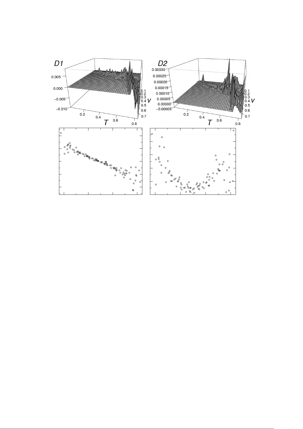
Reconstructing the intermittent dynamics of the tor que in wind turbines Pedr o G. Lind, Matthias W ¨ achter and Joachim Peinke ForW ind - Center for W ind Ener gy Research, Institute of Physics, Carl-v on-Ossietzky Uni versity of Oldenb urg, DE-26111 Oldenbur g, Germany E-mail: pedro.lind@uni-oldenburg.de Abstract. W e apply a framew ork introduced in the late nineties to analyze load measurements in off-shore wind energy con verters (WEC). The frame work is borrowed from statistical physics and properly adapted to the analysis of multiv ariate data comprising wind velocity , po wer production and torque measurements, taken at one single WEC. In particular, we assume that wind statistics driv es the fluctuations of the torque produced in the wind turbine and show how to extract an ev olution equation of the Langevin type for the torque driven by the wind velocity . It is known that the intermittent nature of the atmosphere, i.e. of the wind field, is transferred to the po wer production of a wind energy con verter and consequently to the shaft torque. W e sho w that the derived stochastic differential equation quantifies the dynamical coupling of the measured fluctuating properties as well as it reproduces the intermittenc y observ ed in the data. Finally , we discuss our approach in the light of turbine monitoring, a particular important issue in off-shore wind farms. 1. Introduction While wind energy can be taken as one of the best answers to the world-wide energetic problem[1], due to its particular physical features and turbulent nature it also presents challenging problems to be solved, e ven in more theoretical research fields such as physics and data analysis[2, 3]. One of such open problems is the ability for dev eloping methods that reproduce the particular statistical properties shown in data series of po wer output or wind v elocity measured at one wind turbine or wind ener gy con verter (WEC). As it is known[2], since wind speed presents non-Gaussian fluctuations in time, the power output of one turbine sho ws also this intermittent behavior[4] making predictions of energy production rather dif ficult. Similarly , the intermittenc y of wind speed is also reflected in the torque of the shaft. Moreo ver , the loads applied by the wind on the WEC contrib ute significantly to determine the f atigue beha vior and life expectanc y of WECs[5, 6, 7]. Therefore, establishing good models for the intermittent ev olution of the torque is an important task for better understanding and predicting the energy production and monitor the fatigue loads in WECs. In this paper we focus on the fluctuations of the torque, assuming them as a direct result of atmospheric wind fields sho wing a high frequenc y of extreme events (non Gaussian). Recently , Milan et al[8] have conjectured that the anomalous wind statistics are responsible for the intermittent time e volution of the load, promoting additional fatigue of the turbine itself. Here we sho w that this is indeed the case, by deri ving an e v olution equation for the series of torque measurements that is constrained to the value of corresponding wind speeds. T o this end we use and analyze measurements of wind, power and torque at one WEC of Alpha V entus wind farm at the North Sea. As we sho w below , initializing the differential ev olution equation with the first values of our data series we are able to properly reproduce the time series of the torque as well as its main statistical features, Figure 1. (Left) Location of the R04 WEC at the Alpha V entus wind farm (red bullet) [Photo: Sean Gallup/Getty Images]. (Right) Joint probability density function as a function of the torque and of the wind velocity . All data w as masked through normalization to the lar gest values (see te xt). including its intermittent behavior . Our approach follows from the method proposed in Ref. [4, 8] already applied to the po wer output of single WEC. W e start in Sec. 2 by describing the data analyzed and in Sec. 3 the method is described in further detail. Our results and comparati ve analysis is presented in Sec. 4 and conclusions and further discussions on this topic are gi ven in Sec. 5. 2. Data: the Alpha V entus off-shore wind farm The data analyzed in this paper comprehends three sets of measurements, namely wind speed, po wer output and torque during the full month of January 2013. The data was measured at one WEC of the Alpha V entus wind farm (see Fig. 1, left), also kno wn as Borkum W est. This wind farm is the first off- shore wind f arm in German y and it is located approximately at 54 . 3 o N- 6 . 5 o W . The torque is computed from the measurements of the po wer output P and rotation number n , as T = P /ω , with ω = nπ / 30 the angular v elocity of the operating shaft in units of rotations per minute. The selected WEC w as A V04 from Sen vion, formely RePo wer . The sampling rate of the po wer output and torque is 50 Hz and the sampling rate of the wind speed is 1 Hz. Since we need to use the same sampling rate for all data series, we only consider power and torque measurements at instants for which a velocity measurement also e xists ( 1 Hz). All data series were analyzed according to all confidential protocols and were properly masked through the normalization by their highest v alues. Therefore the scientific conclusions are not af fected by such data protection requirements. The joint probability density function (PDF) ρ ( T , v ) of both the wind speed and torque measurements is sho wn in Fig. 1 (right) and is according to the torque-velocity curv e known in the literature[2, 9]. A time sampling of each data series is plotted in Fig. 2 (left) together with an e xample of one time period where both torque and power change abruptly (right). These abrupt fluctuations are the ones responsible for the intermittent behavior of the wind ener gy production and wind loads which can be easily seen in the increment statistics sho wn in Fig. 3. T o obtain the increment statistics of the torque T we consider torque difference taken within a fixed time-gap τ , namely ∆ T τ ( t ) = T ( t + τ ) − T ( t ) , (1) and similarly for the wind speed and power output. As one sees from Fig. 3, for up to one hour or more, 0 0,2 0,4 0,6 0,8 v 0,25 0,3 0,35 0,4 0 0,2 0,4 0,6 0,8 P 0,25 0,3 0,35 0,4 0,45 1,8e+07 1,9e+07 2e+07 2,1e+07 t 0 0,2 0,4 0,6 0,8 T 1,9384 1,9388 1,9392 t 0,3 0,33 0,36 0,39 0,42 0,45 0,48 0,51 (s) ( 10 7 s) (a) (b) (c) Figure 2. Sketch of time series of (a) the wind velocity v , (b) the power output P and (c) the torque T . On the right a shorter time-interval of each series is plotted to illustrated a stronger fluctuation of power and torque. All data was masked through normalization to the lar gest v alues of v , P and T respectively . the increment distributions are clearly non-Gaussian, particularly the ones of torque and power . It is our purpose to pro vide a reconstruction procedure that reproduces the same intermittent statistics at se veral time scales, in order to better quantify the torque fluctuations. 3. Methodology: the conditioned Langevin approach In 1997 a direct method to extract the e v olution equation of stochastic series of measurements was proposed by Peinke and Friedrich[10]. Since then several applications of this frame work were proposed and de veloped, ranging from turbulence modeling, to medical EEG monitoring and stock markets. F or a re view in this methods see Ref. [11] and references therein. The method was also applied in the context of wind energy , where it was shown its ability to properly define the po wer characteristic of single WECs[8, 12, 13]. The Langevin approach can briefly be described as follows. Assume we have a set of measurements X ( t ) in time t of one particular property x ev olving according to the stochastic equation dx dt = D (1) ( x ) + q D (2) ( x )Γ t , (2) where Γ t is a Gaussian δ -correlated white noise, i.e. h Γ( t ) i = 0 and h Γ( t )Γ( t 0 ) i = 2 δ ij δ ( t − t 0 ) . Equation (2) is usually called a Lange vin equation[11]. W ith such an Ansatz , one separates the deterministic contribution to the e v olution of x , giv en by the function D (1) (the drift), from the stochastic fluctuations -8 -6 -4 -2 0 2 4 6 8 ∆ v 0,0001 1 10000 1e+08 1e+12 τ = 1 s τ = 16 s τ = 64 s τ = 256 s τ = 1024 s τ = 4096 s -12 -8 -4 0 4 8 12 ∆ P -12 -8 -4 0 4 8 12 ∆ T (a) (b) (c) Figure 3. Probability density functions (PDFs) for the increments of (a) the wind velocity ∆ v , (b) the po wer output ∆ P and (c) the torque ∆ T , for dif ferent time-lags τ . The increments are plotted in units of the corresponding standard de viation (see text). The shift in the v ertical axis is for better visualization. incorporated by function D (2) , called the dif fusion. The constant in δ -correlation and the square root in the Lange vin equation are usually chosen for con venience. By simple integration of the Langevin equation, one easily extracts a set of points similar to the sequence of, e.g., the torque measurements in Fig. 2(c). But the problem here is the in verse one: how can we arri ve to a Lange vin equation directly from the analysis of the set of measurements X ( t ) ? The answer has two main steps. The first one concerns to test if there is a time interv al t ` usually called the Mark ov length for which the succession of measurements are Marko vian, i.e. the ne xt v alue only depends on the present one and is independent of the values previous to it. Mathematically , to be Marko vian means to fulfill the condition ρ ( X ( t + t ` ) | X ( t ) , X ( t − t ` ) , X ( t − 2 t ` ) , . . . ) = ρ ( X ( t + t ` ) | X ( t )) , (3) with ρ representing the conditional probability density functions that can be extracted from histograms of the data set. There are simple standard ways to perform this test[11]. When the measurements obe y this Marko v condition the next step can be carried out. Howe ver , in the case the Markov test f ails, for instance in the presence of measurement noise[14], the ne xt step can still be applied, after taking some cautions that we do not mention here. See Ref. [15] for details. The second step, concerns the computation of both D (1) and D (2) that define Eq. (2), done through the corresponding conditional moments, illustrated in Fig. 4: M (1) ( x, τ ) =  X ( t + τ ) − X ( t ) | X ( t )= x  (4a) M (2) ( x, τ ) =  ( X ( t + τ ) − X ( t )) 2 | X ( t )= x  (4b) (4c) where h·| X ( t )= x i symbolizes a conditional av eraging ov er the full measurement period. Figure 4a and 4b shows the first and second conditional moments respectiv ely , for different v alues of the torque, extracted from the data sets in Alpha V entus. As one sees, for the lowest range of values 0 5 10 15 20 25 τ -0,2 -0,16 -0,12 -0,08 -0,04 0 0,04 0,08 0,12 M (1) (T, ) T in [0.68,0.72] T in [0.72,0.76] T in [0.76,0.81] T in [0.81,0.85] T in [0.85,0.90] 5 10 15 20 25 τ 0 0,002 0,004 0,006 0,008 0,01 0,012 0,014 M (2) (T, ) T D (1) T D (2) (a) (b) D (1) (T) 2D (2) (T) τ τ Figure 4. Conditional moments of the (a) first and (b) second order , for different values of the torque. In blue one illustrates the definition of the corresponding Kramers-Moyal coef ficient, drift and dif fusion, sho wn in the insets of (a) and (b) respectiv ely . of τ , the conditional moments depend linearly on τ . Since the two functions in Eq. (2) are, apart one multiplicati ve constant, the deriv ati ve of the two corresponding conditional moments with respect to τ , namely D ( k ) ( x ) = lim τ → 0 1 k ! M ( k ) ( x, τ ) τ , (5) with k = 1 , 2 they can be directly extracted from the data sets. As illustrated in Fig. 4 with dashed lines, for each value T both D (1) ( T ) and D (2) ( T ) are gi ven by the slope of the linear interpolation of the corresponding conditional moments. Important additional insight can be taken from such plots. For instance, the linear fits of the conditional moments (dashed lines) for the lowest range of τ -values typically cross the zero-axis. The absence of an offset for the conditional moments giv es e vidence of the absence of measurement noise[14, 15]. One important assumption ho we ver must be added: the set of measurements must be stationary . This is of course not the case of power and torque series. T o ov erwhelm this shortcoming, Milan et al propose to consider a Langevin equation, but restricted to a sufficiently confined range of wind velocities[16]. Indeed, the statistical moments of the property being addressed are approximately constant if only a narro w range of wind velocities is considered. Such v ariant leads to what we call the conditioned Lange vin equation: dT dt = D (1) ( T , v ) + q D (2) ( T , v )Γ t , (6) where, for our purpose, T represents the torque on the WEC and v is the wind v elocity . 4. Results: Reconstruction of the torque time series and statistics Applying the methodology described in the previous section for ranges of wind velocity within [ ˜ v , ˜ v +∆ v ] with ∆ v = 0 . 5 and ˜ v within the full range of observed values, we deriv e the numerical estimates of the 0,7 0,75 0,8 0,85 T -0,01 -0,005 0 0,005 0,01 D (1) 0,7 0,75 0,8 0,85 T 0 5e-05 0,0001 0,00015 0,0002 0,00025 D (2) Figure 5. (T op) Numerical result for the drift D (1) ( T , v ) and diffusion D (2) ( T , v ) in the Lange vin equation from which the time series of the torque is reconstructed. (Bottom) For the upper range of v alues of the wind v elocity (around rated wind speed) one plots the projection of drift and dif fusion on the T -axis. See text and Fig. 6. drift D (1) and of the dif fusion D (2) in Eq. (6). Figures 5 (top) show the drift and dif fusion coefficients respectiv ely , each one as a function of the wind velocity and of the torque. While for lo w v alues of the velocity , v . 0 . 3 , both coefficients are poorly defined, due to the lack of sampling, in the most sampled range 0 . 3 . v . 0 . 7 (check with Fig. 1) the drift and diffusion depend respectiv ely linearly and quadratically on T . This dependence can be better seen in the two-dimensional plots of Fig. 5 (bottom). Having e xtracted the functional dependence of both coef ficients D (1) and D (2) we are now able to describe the e volution of the torque by k eeping track of the wind v elocity , simply through an Euler-like discrete version of the conditioned Langevin equation. W e take the first measurement of both wind speed and torque as initial conditions for the stochastic equation and integrate it with respect to t using at each integration step the observ ed wind velocity . The reconstructed series are plotted in Fig. 6(a) together with the empirical series of torque measurements. Clearly , the reconstructed series are close to the real measurements. Moreover , the statistical distrib ution of the increments ∆ T τ are also well reproduced for time scales from seconds up to hours (Fig. 6(b)). All in all, from Fig. 6, one can clearly conclude the ability for the conditioned Lange vin model to properly describe the ev olution of the torque in one WEC. 5. Discussion and conclusions In this paper we sho w how to reconstruct the series of torque measurements through a Lange vin model conditioned to the wind v elocity . The model reproduces well not only the series of torque measurements but also the intermittent feature of its increment statistics. It should be noticed that the validity of Eq. (6) 3,2e+05 3,4e+05 3,6e+05 3,8e+05 4e+05 t 0 0,2 0,4 0,6 0,8 T Empirical Reconstruction -15 -10 -5 0 5 10 15 ∆ T 0,0001 0,01 1 100 10000 1e+06 1e+08 PDF (a) (b) τ=4096 τ=1024 τ=256 τ=64 Figure 6. Reconstruction of the torque (in red) of torque measurements (black): (a) The explicit time- series of the torque and (b) the probability density function of the increments (fluctuations) of the torque within dif ferent time-lags. Time is in seconds, and the T orque increments is in units of corresponding standard de viations ( σ τ ). is not fully guaranteed, since P awula condition[17], D (4) = 0 , was not tested. This condition is necessary for assuming a Langevin ev olution equation. Still, e ven in the case Pawula theorem is not fulfilled, the conditioned Langevin equation can be taken as a first approximation of the stochastic ev olution of the torque in one WEC. The reproduction of torque time series of WECs here described is already significant, though the approximations used for the drift and dif fusion coefficients are of first order only (see Fig. 4). Higher order approximations are possible and would improve the reproduction further[18, 19, 20, 21]. In these higher order corrections one considers the numerical values of the drift for the computation of the corresponding dif fusion. A critical remark should be stated at this point: while the model in Eq. (6) properly reproduces the stochastic e v olution of the torque in WECs it depends on the wind velocity measurements. On one hand, nacelle anemometer wind velocity measurements are typically much less accurate than the measurements of other properties on the WEC, such as the pitch angle. On the other hand, being always coupled to a measured property , in this case the wind speed, the conditioned Lange vin equation is not able to pro vide straightforward forecasts of loads e ven in the nearest time horizons. Still, being able to properly describe the ev olution of the torque, one can use it for pro viding additional input information for forecasting models, namely for training neural networks constructed for torque forecast. Another important ne xt step from this study is to ascertain if such an approach can be applied to other kinds of loads in WEC, namely bending moments. These points can contrib ute to improve monitoring protocols of WECs in of f-shore wind farms and will be addressed in the near future as the next steps. Acknowledgments The authors thank Patrick Milan for useful discussions. This work is funded by the German En vironment Ministry as part of the research project “Probabilistic loads description, monitoring, and reduction for the next generation of fshore wind turbines (OWEA Loads)” under grant number 0325577B. Authors also thank Sen vion for pro viding the data here analyzed. References [1] Johnson G 2006 W ind Ener gy Systems (Kansas State Univ ersity) [2] Burton T , Sharpe D, Jenkins N and Bossanyi E 2001 W ind Energy Handbook (W iley) [3] T M ¨ ucke D K and Peinke J 2011 W ind Ener gy 14 301–316 [4] P Milan M W and Peinke J 2013 Phys. Rev . Lett. 110 138701 [5] Ragan P and Manuel L 2007 W ind Engineering 31 83–99 [6] Moriarty P 2008 W ind Ener gy 11 559–576 [7] Freundenreich K and Argyriadis K 2008 W ind Energy 11 589–600 [8] P Milan T M ¨ ucke D K and Peinke J 2013 W ind Ener gy in print [9] P Rinn M W and Peinke J 2013 Private communication [10] Friedrich R and Peinke J 1997 Phys. Rev . Lett. 78 863 [11] Friedrich R, Peinke J, Sahimi M and T abar M 2011 Phys. Rep. 506 87 [12] E Anahua S Barth J P 2008 W ind Ener gy 11 219 [13] Raischel F , Scholz T , Lopes V and Lind P 2013 Physical Review E 88 042146 [14] FBoettcher, JPeink e, DKleinhans, RFriedrich, PGLind and MHaase 2006 Physical Revie w Letters 97 090603 [15] PGLind, MHaase, FBoettcher, JPeink e, DKleinhans and Friedrich R 2010 Physical Revie w E 81 041125 [16] P Milan M W and Peinke J 2013 Private communication [17] Risken H 1984 The F okker-Planck Equation (Heidelberg: Springer) [18] Friedrich R, Siegert S, Peinke J, L ¨ uck S, Siefert M, Lindemann M, Raethjen J, Deuschl G and Pfister G 2000 Phys. Lett. A 271 217 [19] Ragwitz M and Kantz H 2001 Phys. Rev . Lett. 87 254501 [20] Friedrich R, Renner C, Siefert M and Peinke J 2002 Phys. Rev . Lett. 89 149401 [21] Gottschall J and Peinke J 2008 New Journal of Physics 10 083034