Monte Carlo non local means: Random sampling for large-scale image filtering
We propose a randomized version of the non-local means (NLM) algorithm for large-scale image filtering. The new algorithm, called Monte Carlo non-local means (MCNLM), speeds up the classical NLM by computing a small subset of image patch distances, w…
Authors: Stanley H. Chan, Todd Zickler, Yue M. Lu
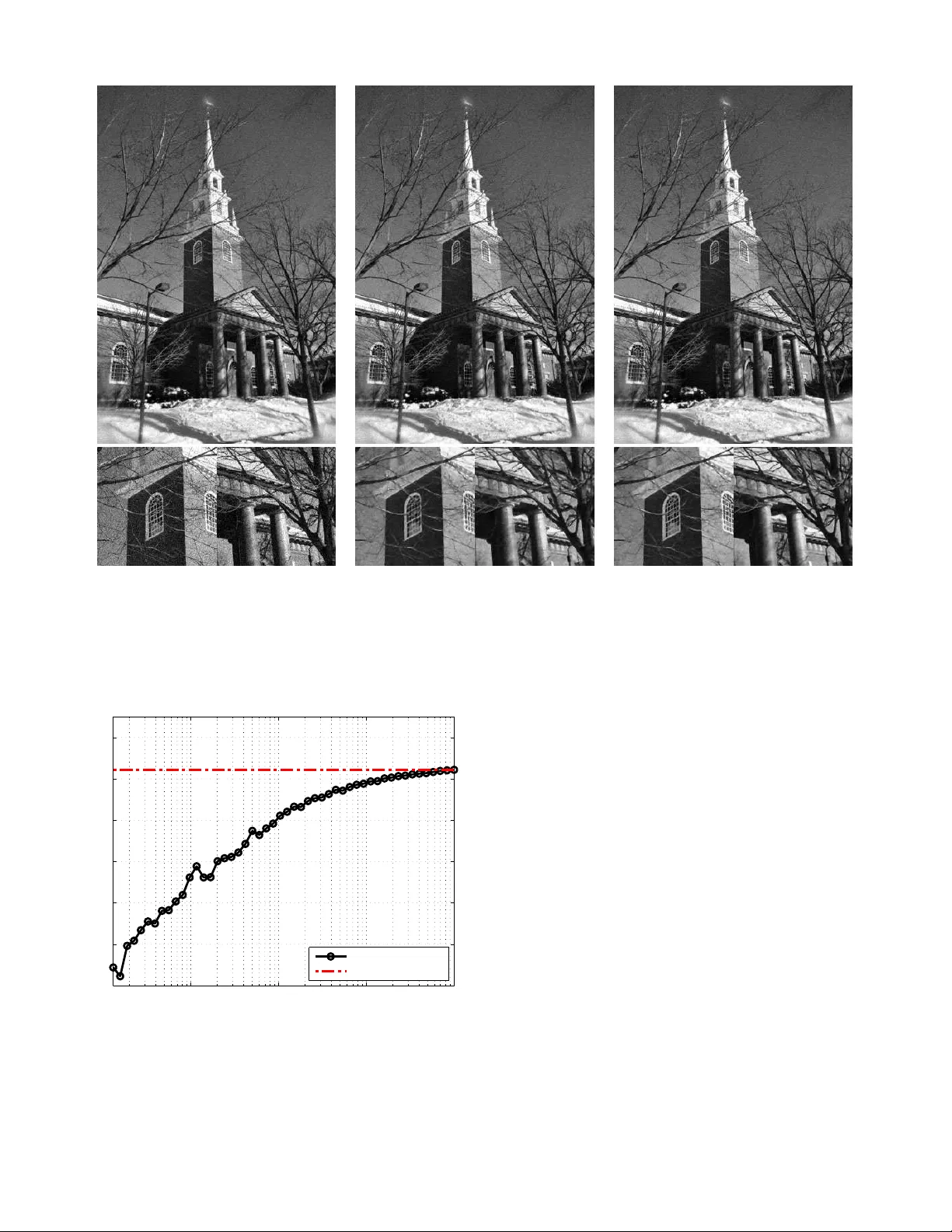
1 Monte Carlo Non-Local Means: Random Sampling for Lar ge-Scale Image Filtering Stanley H. Chan, Member , IEEE, T odd Z ickler , Member , IEEE , and Y ue M. Lu , Se nior Memb er , IEEE Abstract —W e propose a randomized version of th e non-local means (NLM) algorithm f or large-scale image filtering. The new algorithm, called Monte Carlo non -local means (MCNLM), speeds up the classical NLM b y computing a small subset of image patch distances, wh ich are randomly selected according to a designed sampling pattern. W e make two contributions. First, we analyze th e perfor mance of the MCNLM algorithm and show t hat, for large images or large external image databases, the random outcomes of MCNLM are tightly concentrated around the deterministic ful l NLM result. In p articular , our error probability bounds show that, at an y given sampling ratio, the pro bability f or MCNLM to ha ve a larg e deviation from th e original NLM solution decays exponentially as th e size of the image or database gr ows. Second, we deri ve explicit fo rmulas for opti mal sampling patter ns that minimize the error probability bound by exploiting partial knowledge of the pairwise similarity w eights. Numerical experiments show that MCNLM is competitiv e with other state-of-the-art fast NLM algorithms for single-image denoisin g. When appl ied to d enoising images using an external d atabase containing ten billion p atches, MCNLM returns a randomized solution that is within 0.2 dB of the full NLM solution whi le reducin g the r untime by three orders of magnitude. Index T erms —Non-local means, M onte Carlo, p atch-based filtering, sampling, ex ternal denoising, large deviations analysis I . I N T RO D U C T I O N A. B ackgr ound a nd Motivation In recent years, the image proce ssing com munity has wit- nessed a wav e of r esearch aimed at d ev eloping n ew image denoising algorithms that exploit similarities between non - local patches in natural images. Most of these can b e traced back to the non- local means (NLM) d enoising algorith m of Buades et al. [1], [2] pro posed in 200 5. Altho ugh it is no longer the state-of- the-art meth od (see, e.g. , [3], [4] for some more r ecent leading alg orithms), NLM rem ains one of the most influen tial algor ithms in the current denoising literature. Giv en a n oisy image, the NLM algorithm uses two sets of image patches for denoising . Th e first is a set o f noisy patches Y = { y 1 , . . . , y m } , where y i ∈ R d is a d -dim ensional ( i.e. , The authors are with the School of Engineering and Applied Sci- ences, Harv ard Univ ersit y , Cambridge , MA 02138, USA. E-mails: { schan,zickler,yu elu } @seas.harvard. edu . This work wa s support ed in part by the Crouc her Foundat ion Post-doctoral Researc h Fello wship (2012-2013), and in part by the U. S. National Science Founda tion unde r Gra nt CCF-1319140. Prel iminary mate rial in this paper w as presente d at the 38th IEEE Internationa l Conference on Acoustics, Speech and Signal Processing (ICASSP), V ancouv er , May 2013. This paper follo ws the concept of reproducible research. All the results and exa mples presented in the paper are reproducibl e using the code and images av ailable onli ne at htt p://lu.seas.har vard.edu/ . d -pixel) patc h cente red at the i th pixel o f the noisy image. The secon d set, X = { x 1 , . . . , x n } , con tains patches that are o btained f rom som e reference imag es. Conc eptually , NLM simply replaces each i th noisy p ixel with a weig hted a verage of pixels in the r eference set. Specifically , the filtered value at the i th p ixel (for 1 ≤ i ≤ m ) is gi ven by z = P n j =1 w i,j x j P n j =1 w i,j , (1) where x j denotes the value of the center pixel of the j th referenc e patch x j ∈ X , and the weights { w i,j } measure the similarities be tween the patches y i and x j . A stand ard choice for the weigh ts is w i,j = e −k y i − x j k 2 Λ / (2 h 2 r ) , (2) where h r is a scalar parameter deter mined by the n oise level, and k·k Λ is th e weighted ℓ 2 -norm with a diagon al weight matrix Λ , i.e. , k y i − x j k 2 Λ def = ( y i − x j ) T Λ ( y i − x j ) . In most implem entations of NLM (see, e.g. , [5]–[ 11]), the denoising process is ba sed on a single ima ge: the refer ence patches X are the same as the noisy patches Y . W e re fer to this setting, when X = Y , as internal den oising . T his is in contrast to the setting in wh ich the set of referen ce patch es X c ome fro m external image databa ses [12]–[1 4 ], which we refer to as external d enoising . For examp le, 15 , 00 0 images (correspo nding to a ref erence set of n ≈ 10 10 patches) were used in [13], [14]. One theor etical argument for using large- scale external den oising was provid ed in [ 13]: It is shown that, in th e limit of large referenc e sets ( i.e. , when n → ∞ ), external NLM converges to the minimum mean squared error estimator of the und erlying clean images. Despite its strong p erform ance, NLM has a limitation of high computational complexity . It is easy to s ee that computing all the weigh ts { w i,j } re quires O ( mnd ) arith metic oper ations, where m, n, d are, respectively , th e num ber of pixels in th e noisy im age, the number of ref erence p atches u sed, and the patch d imension. Additionally , abo ut O ( mn ) o perations are needed to car ry out th e su mmations and m ultiplications in (1) for all pixels in th e imag e. In the case of intern al denoising , these number s are non trivial sin ce current digital photog raphs can easily contain tens of millions of pixels ( i.e . , m = n ∼ 10 7 or g reater). For external denoising with large reference sets ( e.g. , n ∼ 10 10 ), the com plexity is even m ore o f an issue, making it very challenging to f ully utilize the vast numbe r of images that ar e readily available o nline and po tentially useful as external databases. 2 B. R elated W ork The high complexity of N LM is a well-known challenge. Previous metho ds to speed u p NLM can be ro ughly classified in the fo llowing categories: 1. Reducing the r eference set X . If searching throu gh a large set X is com putationally intensi ve, one natural solutio n is to pre-select a subset of X an d p erform computation o nly on th is subset [1 5]–[17]. For example, fo r inter nal den oising, a spatial weight w s i,j is often inc luded so that w i,j = w s i,j · e −k y i − x j k 2 Λ / (2 h 2 r ) | {z } w r i,j . (3) A common choice of the spatial weig ht is w s i,j = ex p {− d 2 i,j / (2 h 2 s ) } · I { d ′ i,j ≤ ρ } , (4) where d i,j and d ′ i,j are, respectively , the Eu clidean distance and the ℓ ∞ distance between the spatial locations of th e i th and j th pixels; I is the in dicator func tion; and ρ is the width of the spatial search window . By tunin g h s and ρ , one can adjust the size of X acc ording to the heuristic tha t n earby patch es are more likely to be similar . 2. Reducin g dimension d . The patch d imension d can be reduced by se veral method s. First, SVD p rojection [1 0], [18]– [20] can be used to project the d -dim ensional p atches onto a lower dimension al space spanned by the principal c ompon ents computed from X . Seco nd, the integra l image me thod [2 1]– [23] can b e used to fur ther speed up the c omputatio n of k y i − x j k 2 Λ . Th ird, by assum ing a Gaussian m odel on the p atch data, a probab ilistic early termin ation scheme [2 4] can be used to stop compu ting the squared patch difference be fore go ing throug h all the pixels in the pa tches. 3. Optimizing data structur es. The third class of meth ods embed the p atches in X and Y in som e form of optimized data structures. Some examp les include the fast bilateral gr id [25], the fast Gaussian tran sform [26], the Gaussian KD tree [27], [28], th e adap tiv e manifold method [ 29], an d the ed ge patch dictionary [30]. T he data structur es u sed in these algo rithms can sign ificantly r educe the co mputation al complexity of the NLM algo rithm. Howe ver, building th ese data structur es often requires a le ngthy pre- processing stage, or require a large amount of memor y , thereby p lacing limits o n o ne’ s ab ility to u se large refe rence patch sets X . For example, building a Gaussian KD tree requir es the storage of O ( nd ) do uble precision numbers (see, e.g. , [28], [31].) C. Contributions In this paper , we prop ose a rand omized alg orithm to reduce the com putationa l comp lexity o f NLM for b oth in ternal and external deno ising. W e call the metho d Monte Carlo Non - Local Means (MCNLM) , and the basic idea is illustrated in Figure 1 for the case of inter nal denoising . For each pixel i in the noisy image, we randomly select a set of k r eference pixels accor ding to some samplin g p attern and compu te a k -subset of the weights { w i,j } n j =1 to form an appro ximated solution to (1). The com putation al co mplexity of MCNLM is O ( mk d ) , which can be significantly lower than the origin al complexity O ( mnd ) when only k ≪ n weights are compu ted. + + + + + + + + + + + + + + + + + + + + + + + + + + + + + + + + + + + + + + + + + + + + + + + + + + + + + + + + + + + + + + + + + + + + + + + + + + + + + + + + + + + + + + + + + + + + + + + + + + + + + + + + + + + + + + + + + + + + + + + + + + + + + + + + + + + + + + + + + + + + + + + + + + + + + + + random sam ples { w i,j 1 , . . . , w i,j k } Fig. 1: Illu stration of the pr oposed MCNLM algo rithm fo r internal denoising : W e rand omly select, accord ing to a given sampling pattern, a set of k weights { w i,j 1 , . . . , w i,j k } , and use these to com pute a n approximation of the f ull NLM resu lt in (1). The outpu t of MCNLM is rando m. Ho wev er , as the size of the prob lem ( i.e. , n ) gets larger , these rand om estimates become tightly co ncentrated ar ound the tru e re sult. Furthermo re, since there is no need to re-organize the data, th e memory r equireme nt of MCNLM is O ( m + n ) . Th erefore, MCNLM is scalable to large referen ce patch sets X , as we will demonstrate in Section V. The tw o main contributions o f this paper are as follows. 1. P erformance g uarantee . MCNLM is a rando mized algo- rithm. It would not be a useful on e if its rando m ou tcomes fluctuated widely in different executions on the same inpu t data. In Section III, we ad dress this c oncern by sho wing that, as the size of the re ference set X increases, the randomized MCNLM solu tions beco me tightly co ncentrated aro und the original NLM solution. In particular, we show in Theo rem 1 (and Proposition 1) that, for an y given sampling pattern , the probab ility o f having a large deviation from the o riginal NLM solution drops expo nentially as the size o f X g rows. 2. Optimal sampling p atterns . W e derive optimal sampling patterns to min imize the approx imation error pr obabilities established in our perfor mance analysis. W e show that seeking the optimal samplin g pattern is equiv alent to solving a variant of the classical water-filling p roblem, for which a c losed-for m expression ca n be fou nd (see Th eorem 2). W e also present two pr actical samp ling p attern designs that exploit par tial knowledge of the pairwise similarity weights. The rest of the pape r is organ ized as follows. After present- ing the MCNLM algorithm and discuss its basic pro perties in Section II, we analy ze the p erform ance in Section III and derive the optimal sampling p atterns in Section IV. Ex peri- mental results are g i ven in Section V, and co ncludin g remark s are gi ven in Section VI . I I . M O N T E C A R L O N O N - L O C A L M E A N S Notatio n: Throug hout the pap er , we use m to denote the number of pixels in the noisy image, and n the n umber patches in the referen ce set X . W e u se up per-case letters, such as X , Y , Z , to represent rand om variables, an d lower -case letter s, such as x, y , z , to represen t deterministic v ariables. V ectors are represented by b old letters, and 1 denotes a co nstant vector of which all entries are one. Fina lly , for n otational simplicity in presen ting our theoretica l analysis, we assume th at all pixel intensity v alues h av e b een normalized to the range [0 , 1] . CHAN et al. : MONT E-CARLO NON-LOCAL MEANS 3 A. Th e Sampling Pr ocess As discussed in Section I, comp uting all the weights { w i,j } 1 ≤ i ≤ m, 1 ≤ j ≤ n is c omputatio nally proh ibitiv e wh en m and n are large. T o reduce the comp lexity , the basic idea o f MCNLM is to random ly select a su bset of k representatives of { w i,j } (referr ed to as samp les) to appro ximate the sum s in the numer ator and denom inator in (1). The samp ling process in the p roposed algo rithm is applied to each of the m pixels in the noisy image indep endently . Since the sampling step and subsequen t computatio ns ha ve the same fo rm for each pixel, we shall drop the pixel ind ex i in { w i,j } , writing the weights as { w j } 1 ≤ j ≤ n for n otational simplicity . The samplin g pro cess of MCNLM is determ ined by a sequence o f indepen dent rand om variables { I j } n j =1 that take the value 0 or 1 with the follo wing p robabilities Pr[ I j = 1] = p j and Pr[ I j = 0] = 1 − p j . (5) The j th weight w j is sampled if and only if I j = 1 . I n what follows, we assume tha t 0 < p j ≤ 1 , and refer to the vector of all these pro babilities p def =[ p 1 , . . . , p n ] T as the sampling pattern of the algo rithm. The ratio between the nu mber o f samples taken an d th e number of r eference patches in X is a ran dom v ariable S n = 1 n n X j =1 I j , (6) of which the expected v alue is E [ S n ] = 1 n n X j =1 E [ I j ] = 1 n n X j =1 p j def = ξ . (7) W e ref er to S n and ξ as the empirical sampling ratio and the a verage sampling ratio , respectively . ξ is an importan t parameter of the MCNLM algorithm. Th e original (o r “fu ll”) NLM correspo nds to the setting when ξ = 1 : In th is case, p = 1 def = [1 , . . . , 1 ] T , so that all the samples are selected with probab ility one. B. Th e MCNLM Alg orithm Giv en a set of random samp les fro m X , we approx imate the numerato r and denominato r in (1) by two random variables A ( p ) def = 1 n n X j =1 x j w j p j I j and B ( p ) def = 1 n n X j =1 w j p j I j , (8) where the ar gument p emphasizes the fact that the distrib utions of A and B are de termined by the sampling pattern p . It is easy to comp ute the expected values of A ( p ) and B ( p ) as µ A def = E [ A ( p )] = 1 n n X j =1 x j w j , (9) µ B def = E [ B ( p )] = 1 n n X j =1 w j . (10) Thus, up to a commo n mu ltiplicativ e constan t 1 /n , the two random variables A ( p ) and B ( p ) are u nbiased estimates of the true numerator and denomin ator, respectively . Algorithm 1 Mo nte Carlo No n-local Means (MCNLM) 1: For each n oisy pixel i = 1 , . . . , m , do the followings. 2: In put: Noisy pa tch y i ∈ Y , databa se X = { x 1 , . . . , x n } and sampling p attern p = [ p 1 , . . . , p n ] T such that 0 < p j ≤ 1 , and P n j =1 p j = nξ . 3: Ou tput: A ran domized e stimate Z ( p ) . 4: for j = 1 , . . . , n do 5: Generate a random variable I j ∼ Bernoulli ( p j ) . 6: If I j = 1 , then co mpute the weigh t w j . 7: end for 8: Com pute A ( p ) = 1 n P n j =1 w j x j p j I j . 9: Com pute B ( p ) = 1 n P n j =1 w j p j I j . 10: Outp ut Z ( p ) = A ( p ) /B ( p ) . The full NLM result z in (1) is then appro ximated by Z ( p ) def = A ( p ) B ( p ) = P n j =1 x j w j p j I j P n j =1 w j p j I j . (11) In gen eral, E [ Z ( p )] = E h A ( p ) B ( p ) i 6 = E [ A ( p )] E [ B ( p )] = z , an d thus Z ( p ) is a biased estimate of z . Howev er , we will sh ow in Section III that the pro bability of ha ving a large deviation in | Z ( p ) − z | d rops exponentially as n → ∞ . Thus, for a large n , the MCNLM solu tion ( 11) can still f orm a very accurate approx imation of the original NLM solution (1). Algorithm 1 sho ws the pseudo-co de of MCNLM for internal denoising . W e n ote that, except for th e Bernou lli sampling process, all o ther steps are identical to th e o riginal NLM. Therefo re, MCNLM can be thoug ht of as add ing a com ple- mentary sampling process on to p of the o riginal NLM. The marginal cost of implementation is thus minimal. Example 1: T o empirically d emonstrate the usef ulness of the simple sampling mechan ism of MCNLM, we apply the algorithm to a 1072 × 712 imag e shown in Figure 2(a). Here, we u se X = Y , with m = n ≈ 7 . 6 × 1 0 5 . I n this experiment, we let the noise be i.i.d . Gaussian with zero mean and standar d deviation σ = 15 / 25 5 . The patch size is 5 × 5 . In computing the similarity w eights in ( 3) and (4), we set the param eters as follows: h r = 15 / 255 , h s = ∞ , ρ = ∞ ( i.e. , no spatial windowing) and Λ = 1 25 I . W e choose a unifor m sampling pattern, i.e., p = [ ξ , . . . , ξ ] T , for som e sam pling ratio 0 < ξ < 1 . The re sults of this experiment are shown in Figure 2 and Figure 3. Th e peak signal-to -noise ratio (PSNR) curve detailed in Figure 3 shows that MCNLM conv erges to its limiting value rapidly as the sampling ratio ξ approa ches 1 . For examp le, at ξ = 0 . 1 ( i.e. , a roug hly ten-fold reduction in co mputation al complexity), MCNLM achieves a PSNR that is only 0 . 2 d B away from the full NL M result. More n umerical e xperimen ts will be presen ted in Section V. I I I . P E R F O R M A N C E A N A L Y S I S One fu ndamenta l q uestion abou t MCNLM is whether its random estimate Z ( p ) as define d in (11) will be a g ood approx imation of the full NLM so lution z , especially wh en the sampling r atio ξ is small. In this sectio n, we an swer this 4 noisy (24.60 dB) ξ = 0 . 005 (27.58 dB) ξ = 0 . 1 (28.90 dB) Fig. 2: Denoising an image of size 1072 × 712 b y MCNLM with u niform samp ling. ( a) The original imag e is corrupted with i.i.d. Gaussian no ise with σ = 15 / 2 55 . (b) and ( c) Denoised imag es with samplin g ratio ξ = 0 . 005 and ξ = 0 . 1 , respecti vely . Shown in parenthesis are the PSNR v alues (in dB) av eraged ov er 100 trials. 10 −3 10 −2 10 −1 10 0 24 25 26 27 28 29 30 ξ PSNR (dB) Monte Carlo NLM Classical NLM Fig. 3: PSNR as a function of th e a verag e sampling ratio ξ . The “circled” line indicates th e result of MCNLM. The horizon tal line in dicates the result of the full NLM ( i.e. , MCNLM at ξ = 1 ). Note that at ξ = 0 . 1 , MCNLM achieves a PSNR that is only 0 . 2 dB b elow the full NLM result. Add itional experiments ar e p resented in Sectio n V. question by pr oviding a rigoro us analy sis o n the a pprox imation error | Z ( p ) − z | . A. La r ge Deviations Bo unds The mathem atical tool we use to analyze the propo sed MCNLM alg orithm come s from the pro babilistic lar ge de- viations theo ry [32]. This theory has be en widely used to quan tify the following pheno menon: A smoo th fun ction f ( X 1 , . . . , X n ) of a large nu mber of indepen dent rando m variables X 1 , . . . , X n tends to concentrate very tigh tly around its mean E [ f ( X 1 , . . . , X n )] . Roughly speaking, th is concen- tration phe nomeno n happens bec ause, while X 1 , . . . , X n are individually random in n ature, it is unlikely f or m any of them to work collabor ativ ely to alter the overall system by a sign ificant amo unt. Thus, for la rge n , the rando mness of these variables tends to be “canceled out” and the functio n f ( X 1 , . . . , X n ) stays roughly con stant. T o gain insights f rom a concrete examp le, we first apply th e large deviations th eory to stud y the empirical sampling ratio S n as defined in (6). Here, the indepen dent rand om variables are the Bernoulli r andom variables { I j } 1 ≤ j ≤ n introdu ced in (5), and the smooth function f ( · ) computes th eir a vera ge. It is well known fro m the law of large numb ers (LLN) that the empirical mean S n of a large number of in depend ent random variables stays very clo se to the true mean, which is CHAN et al. : MONT E-CARLO NON-LOCAL MEANS 5 0 0.02 0.04 0.06 0.08 0.1 10 −8 10 −6 10 −4 10 −2 10 0 10 2 10 4 ε Pr[ S n − E [ S n ] > ε ] True probabilities Law of large numbers bounds Large deviations bounds Fig. 4: Com paring th e large deviations bound (13), the LLN bound ( 12), and the true e rror p robab ility Pr[ S n − E [ S n ] > ε ] as estimated by Monte Carlo simulations. Fixing n = 10 6 , we plot the b ound s and probabilities for different values of ε . equal to the average sampling ratio ξ in ou r case. In particular, by the standard Cheby shev inequality [ 33], we kn ow that Pr[ S n − E [ S n ] > ε ] ≤ Pr[ | S n − E [ S n ] | > ε ] < V ar[ I 1 ] nε 2 , (12) for e very positive ε . One drawback o f th e bound in (12) is that it is overly loose, providing on ly a linear r ate of decay for the error prob abilities as n → ∞ . In contrast, the large d eviations theo ry p rovides many powerful p robability ine qualities which of ten lead to much tigh ter boun ds with exponen tial d ecays. In this work, we will use one particular inequality in the large deviations theory , due to S. Bernstein [34]: Lemma 1 (B ernstein Inequality [34]): Let X 1 , . . . , X n be a sequence of independen t r andom variables. Suppose that l j ≤ X j ≤ u j for a ll j , wher e u j and l j are constants. Let S n = (1 /n ) P n j =1 X j , an d M = max 1 ≤ j ≤ n ( u j − l j ) / 2 . Th en for e very positive ε , Pr [ S n − E [ S n ] > ε ] ≤ exp − nε 2 2 1 n P n j =1 V ar[ X j ] + M ε/ 3 . (13) T o see how Bernstein’ s inequ ality can gi ve us a better pr oba- bility bound for the emp irical sampling ratio S n , we note that X j = I j in o ur case. Thus, M = 1 and E [ S n ] = ξ . Mor eover , if th e sampling pattern is un iform, i.e. , p = [ ξ , . . . , ξ ] T , we have 1 n P n j =1 V ar[ X j ] = 1 n P n j =1 p j (1 − p j ) = ξ (1 − ξ ) . Sub- stituting these num bers into (13) yields an exponentia l u pper bound on the erro r probab ility , which is plotted and compared in Figure 4 ag ainst the LLN bound in (12) an d a gainst th e tru e probab ilities estimated b y M onte Carlo simulation s. It is clea r that the expon ential bo und provided by Bernstein’ s inequality is much tig hter than that provided by LLN. B. Ge neral Err or P r ob ability Bound for MCNLM W e now derive a gener al boun d for the error pr obabilities of MCNLM. Specifically , for any ε > 0 and any sampling pattern p satisfying the cond itions that 0 < p j ≤ 1 and 1 n P n j =1 p j = ξ , we want to study Pr [ | Z ( p ) − z | > ε ] , (14) where z is the full NLM result defin ed in (1) and Z ( p ) is the MCNLM e stimate defined in (11). Theor em 1 : Assum e that w j > 0 for all j . Then for every positive ε , Pr [ | Z ( p ) − z | > ε ] ≤ exp {− nξ } + e xp − n ( µ B ε ) 2 2 1 n P n j =1 α 2 j 1 − p j p j + ( µ B ε ) M α / 6 + e xp − n ( µ B ε ) 2 2 1 n P n j =1 β 2 j 1 − p j p j + ( µ B ε ) M β / 6 , (15) where µ B is the average similarity weigh ts defined in (10), α j = w j ( x j − z − ε ) , β j = w j ( x j − z + ε ) , and M α = max 1 ≤ j ≤ n | α j | p j , and M β = max 1 ≤ j ≤ n | β j | p j . Pr oo f: See App endix A. Remark 1: In a prelimin ary versio n of o ur work [35], we presented, based on the idea of martingale s [36], an erro r probab ility b ound for the special case wh en the sampling pattern is u niform . The result of Theo rem 1 is mo re g eneral and applies to any sampling patterns. W e also note that the bound in (15) quan tifies the deviation o f a ratio Z ( p ) = A ( p ) /B ( p ) , where the nu merator an d denom inator are bo th weighted sums of independ ent rand om v ariables. It is therefor e more g eneral than the ty pical conc entration bound s seen in the literature (see, e.g . , [37], [38]), where only a sing le weighted sum of rand om variables ( i.e. , either the nu merator or the denomin ator) is considered . Example 2: T o illustrate the result of Theorem 1, we con- sider a one-d imensional signal as shown in Fig ure 5(a). The signal { x j } n j =1 is a piecewise continuo us fu nction corru pted by i.i.d. Gaussian noise. The noise standard deviation is σ = 5 / 255 and the signal length is n = 10 4 . W e use MCNLM to denoise the 5001 - th pixel, and the samp ling pattern is uniform with p j = ξ = 0 . 05 fo r all j . For ε = 0 . 01 , we can com pute that 1 n P n j =1 α 2 j = 1 . 335 × 10 − 4 , 1 n P n j =1 β 2 j = 1 . 452 × 10 − 4 , µ B = 0 . 3015 , M α = 0 . 458 , and M β = 0 . 617 . It then fo llows from (15) th at Pr[ | Z ( p ) − z | > 0 . 01] ≤ 6 . 51 6 × 10 − 6 . This boun d shows th at the ran dom MCNLM estimate Z ( p ) , obtained by taking o nly 5% of the sam ples, stays within one per cent of the tru e NLM result z with overwhelming probab ility . A co mplete rang e of results fo r d ifferent values 6 0 2000 4000 6000 8000 10000 0 0.1 0.2 0.3 0.4 0.5 0.6 0.7 j x j si g n a l { x j } n j =1 0 0.05 0.1 0.15 0.2 0 0.5 1 1.5 2 ε Pr [ | Z ( p ) − z | > ε ] sam p lin g p ro b a b ilit y p j = 0 . 0 5 Large deviations bounds True probabilities 0 0.002 0.004 0.006 0.008 0.01 0 0.5 1 1.5 2 Zoom−in view (a) Noisy signal { x j } n j =1 (b) Probability P r[ | Z ( p ) − z | > ε ] Fig. 5: Ex ample to illustrate Theo rem 1. (a) A o ne-dimen sional sign al with length n = 1 0 4 , corrup ted by i.i.d. Ga ussian noise with σ = 5 / 255 . W e use the MCNLM algorithm to den oise th e sig nal. The patch size is d = 5 and the parameters are h r = 15 / 255 and h s = ∞ , respectiv ely . (b) The error pro bability as a fu nction of ε . In th is plot, the “crosses” d enote the true probabilities a s estimated b y 10 5 indepen dent trials and the “circles” denote the an alytical upper bound p redicted by Theorem 1. For easy comparisons, we also provide a zoomed-in v ersion of th e p lot in the insert. of ε are shown in Figure 5(b), where we compa re the true error probab ility as estimated by Mon te Carlo simulations with the analy tical upp er b ound pred icted by Theorem 1. W e see from the “zoom ed-in” portion of Figure 5(b) that the analytical bound approach es the true pr obabilities f or ε ≥ 0 . 005 . C. Special Case: Un iform S ampling P atterns Since the error probab ility boun d in (15) holds for all sampling p atterns p , we will use (15) to design o ptimal nonun iform sampling pattern s in Sec tion IV. But before we discuss th at, we first con sider the special case where p is a unifor m sampling p attern to p rovide a c onv enient and easily interpretab le bou nd on the error p robabilities. Pr op osition 1 (Unifo rm S ampling) : Assum e that the sam- pling pattern is unifo rm, i.e. , p = ξ 1 . Then fo r every ε > 0 and e very 0 < ξ ≤ 1 , Pr [ | Z ( p ) − z | > ε ] ≤ exp {− n ξ } + 2 exp {− nµ B f ( ε ) ξ } , (16) where f ( ε ) def = ε 2 / 2(1 + ε )(1 + 7 ε/ 6) . T o interpr et (16), we note th at, for large n , the first te rm on the righ t-hand side o f (16) is negligible. For example, when n = 10 4 and ξ = 0 . 01 , we have e − nξ = 3 . 7 × 10 − 44 . Thu s, the error p robab ility bou nd is do minated by the second term, whose negati ve exponent is determined by fo ur factors: 1. The size of the r eference set X . If all other par ameters are kept fixed or strictly bounded below b y so me positive constants, the erro r probability goes to zero as an expo nential function of n . This shows that the random estimates ob tained by MCNLM can be very ac curate, when the size of the image (f or inter nal den oising) or the size o f th e diction ary (for external deno ising) is large. 2. S ampling ratio ξ . T o reduce the samp ling ra tio ξ wh ile still keeping the e rror prob ability small, a larger n , inversely propo rtional to ξ , is needed. 3. Precision ε . Note that th e fun ction f ( ε ) in ( 16) is of order O ( ε 2 ) fo r small ε . Thus, with all other terms fixed, a k -fold reduction in ε requires a k 2 -fold increase in n or ξ . 4. P atch r edunda ncy µ B . Recall th at µ B = 1 n P n j =1 w j , with the weig hts { w j } measuring the similar ities between a noisy p atch y i and all patche s { x j } n j =1 in the re ference set X . Thus, µ B serves as an ind irect m easure o f th e n umber of patches in X th at are similar to y i . If y i can find many similar (redunda nt) p atches in X , its corr espondin g µ B will be large an d so a relatively small n will be sufficient to make the probability small; and vice versa. Using the simplified expre ssion in (16), we d erive in Ap- pendix C the following upper b ound on the mean squared erro r (MSE) of the MCNLM estimation: Pr op osition 2 (MSE ): Let th e sampling pattern be unifo rm, with p = ξ 1 . Then for a ny 0 < ξ ≤ 1 , MSE p def = E p h ( Z ( p ) − z ) 2 i ≤ e − nξ + 1 nξ 52 3 µ B . (17) Remark 2: The above result indicates that, with a fixed av erage sampling ratio ξ and if the patch redun dancy µ B is bound ed from b elow by a positi ve constant, then the MSE of the MCNLM estimation conver ges to zero as n , the size o f the reference set, goes to infinity . Remark 3: W e note that the MSE p stated in Proposition 2 is a me asure o f th e deviation between the r andomiz ed solution Z ( p ) and the deter ministic (fu ll NLM) solution z . I n oth er words, th e expectation is taken over the dif ferent r ealizations of th e samp ling pattern, with the noise (and thus z ) fixed. Th is CHAN et al. : MONT E-CARLO NON-LOCAL MEANS 7 is different from the standard M SE used in image processing (which we deno te by MSE η ), where the expectation is taken over different noise realizations. T o make this po int more precise, we defin e z ∗ as th e grou nd truth noise free image, Z ( p , η ) as th e MCNLM so lution using a random sampling pattern p for a p articular noise realization η . No te that the fu ll NLM result can be written as Z ( 1 , η ) ( i.e. wh en the sampling pattern p is the all-on e vector .) W e consider the f ollowing two q uantities: MSE η = E η [( Z ( 1 , η ) − z ∗ ) 2 ] (18) and MSE η, p = E η, p [( Z ( p , η ) − z ∗ ) 2 ] (19) The fo rmer is the MSE ach iev ed by th e full NLM, whereas the latter is the MSE achieved by the propo sed MCNLM. While we do not have the oretical b ound s linking MSE η to MSE η, p (as do ing so wou ld re quire th e kn owledge of the groun d truth im age z ∗ ), we refe r the read er to T ab le I in Sec. V, where num erical simulations show that, even fo r relatively small sampling ratios ξ , the MSE achieved by MCNLM stays fairly clo se to the MSE achieved by the full NLM. I V . O P T I M A L S A M P L I N G P A T T E R N S While the un iform sampling scheme ( i.e. , p = ξ 1 ) allows for easy analysis and provides useful insigh ts, the perf ormanc e of the propo sed MCNLM algorith m can be significantly improved by using pr operly chosen nonu niform samp ling patterns. W e pre sent the design o f such p atterns in this sectio n. A. De sign F ormulation The startin g po int of seek ing an optimal samplin g patter n is the gen eral probability bound provided b y Theor em 1. A challenge in applying this pro bability boun d in practice is th at the right-han d side of (15) in v olves the com plete set of weights { w j } and the full NLM result z . One can of course compute these values, b ut doing so will def eat the purpo se of random sampling, which is to speed up NL M by not co mputing all the weights { w j } . T o address this pr oblem, we assume that 0 < w j ≤ b j ≤ 1 , (20) where the upper boun ds { b j } are either known a p riori or can be efficiently co mputed. W e will p rovide concr ete examples of such upper bound s in Section IV -B. For now , we assum e that the b ounds { b j } hav e alre ady b een obtained. Using (2 0) and notin g that 0 ≤ x j , z ≤ 1 (and thus | x j − z | ≤ 1 ), we can see that the p arameters { α j , β j } in (15) are bound ed by | α j | ≤ b j (1 + ε ) and | β j | ≤ b j (1 + ε ) , respectively . I t then fo llows from (15) th at Pr [ | Z ( p ) − z | > ε ] ≤ exp {− nξ } + 2 exp − n ( µ B ε ) 2 / (1 + ε ) 2 2 1 n P n j =1 b 2 j 1 − p j p j + M max 1 ≤ j ≤ n b j p j , (21) where M def = ( µ B ε ) / (6(1 + ε )) . Giv en the a verage samplin g ratio ξ , we seek samplin g pat- terns p to minimize the probab ility b ound in (21), so th at the random MCNLM estimate Z ( p ) will be tig htly co ncentrated around the full NLM result z . Equiv alently , we solve the following optimiza tion prob lem. ( P ) : arg min p 1 n P n j =1 b 2 j 1 − p j p j + M max 1 ≤ j ≤ n b j p j sub ject to 1 n n P j =1 p j = ξ and 0 < p j ≤ 1 . (22) The o ptimization for mulated has a clo sed-form solution stated as b elow . The d eriv ation is gi ven in Append ix D. Theor em 2 (Optimal Sampling P atterns): The solu tion to ( P ) is gi ven by p j = max(min( b j τ , 1) , b j /t ) , for 1 ≤ j ≤ n, (23) where t def = max 1 nξ P n j =1 b j , max 1 ≤ j ≤ n b j , and the parameter τ is chosen so that P j p j = nξ . Remark 4: It is easy to verify th at the fun ction g ( x ) = n X j =1 max(min( b j x, 1) , b j /t ) − nξ (24) is a piecewise linear an d monoton ically increasing function . Moreover , g (+ ∞ ) = n (1 − ξ ) > 0 and g (0) = n X j =1 b j t − n ξ ≤ P n j =1 b j 1 nξ P n j =1 b j − n ξ = 0 . Thus, τ can be unique ly determ ined as the root of g ( τ ) . Remark 5: The cost fu nction of ( P ) contain s a quan tity M = ( µ B ε ) / (6(1 + ε )) . On e po tential issue is that th e two parameters ( µ B and ε ) that are not necessarily known to the algorithm . Howe ver , as a remarkab le pro perty of the solution giv en in Theorem 2 , th e o ptimal samp ling p attern p does not depend on M . Th us, o nly a single parame ter , namely , the av erage sampling ratio ξ , will be neede d to fully sp ecify the optimal sampling pa ttern in practice. B. Op timal Sampling P atterns T o construct the o ptimal sampling p attern prescribed b y Theorem 2, we need to find { b j } , which are the upper bo unds on the tru e similarity weigh ts { w j } . At o ne extreme, the tightest upp er boun ds are b j = w j , but this o racle schem e is not realistic as it req uires that we k now all the weights { w j } . At the o ther extreme, we can use the trivial upper boun d b j = 1 . It is easy to verify that, und er this setting, the sampling pattern in (4 0) b ecomes the unifo rm pattern, i.e. , p j = ξ for all j . In what follows, we pr esent two choices for the uppe r bound s th at can be efficiently com puted and that can utilize partial knowledge of w j . 1) Bou nds fr om spatial information : The first u pper bound is designed fo r internal ( i.e. , single image) denoising wher e there is of ten a spatial term in the similarity weight, i.e. , w j = w s j w r j . (25) 8 One example o f the spatial weight can be fou nd in ( 4). Sin ce w r j ≤ 1 , we alw ays h av e w j ≤ w s j . T hus, a possible choice is to set b s j = w s j . (26) The advantage of the above upper boun d is that b s j is a function of the spatial distanc e d i,j between a pair of pixels, which is independ ent of th e image data X and Y . Therefore, it can be pre-comp uted befo re running th e MCNLM algorithm. Moreover , since { b j } is sp atially in variant , they can be reused at all p ixel locatio ns. 2) Bound s fr o m intensity info rmation: For external image denoising , th e patch es in X and Y do not h av e any spatial relationship, as they can come fr om different images. I n this case, the similarity weig ht w j is on ly due to th e difference in pixel intensities ( i.e. , w j = w r j ), and thus we can not use the spatial bo unds given in (26). T o d erive a new bound for this case, we first recall the Cauchy-Schwartz in equality: For any two vectors u , v ∈ R d and f or any positive-definite weig ht matrix Λ ∈ R d × d , it h olds that | u T Λ v | ≤ k u k Λ k v k Λ . Setting u = y − x j , we then have w j = e −k y − x j k 2 Λ / (2 h 2 r ) ≤ e − ( ( x j − y ) T Λ v ) 2 / ( 2 h 2 r k v k 2 Λ ) ≤ e − ( x T j s − y T s ) 2 = b r j , (27) where s def = Λ v / √ 2 h r k v k Λ . The vector v can be any no nzero vector . In practice, we choose v = 1 with Λ = diag { 1 / d, . . . , 1 /d } and we fin d this ch oice e f- fective in our n umerical experimen ts. In this case, b r j = exp − ( x T j 1 − y T 1 ) 2 / (2 d 2 h 2 r ) . Remark 6: T o obtain the upper bound b r j in (27), we need to compute the terms y T s and x T j s , which are the pro jections o f the vectors y and x j onto the one-dimen sional sp ace sp anned by s . These p rojections can be efficiently computed by con- volving the noisy image and the images in the refer ence set with a spatially-limited kernel correspon ding to s . T o further reduce the com putation al complexity , we also adopt a two- stage importan ce sampling proc edure in our implem entation, which allows u s to av oid the computation of the e xact values of { b j } at most p ixels. Details of our implementation are given in a supplementary technical report [39]. Remark 7: Given the o racle samp ling patter n, it is possible to improve the performan ce of NLM b y deterministically choosing the weights accordin g to the oracle sampling p attern. W e refer the read er to [1 1], where similar approache s based on spatial ad aptations were pro posed. Example 3: T o dem onstrate th e p erform ance of the various sampling patter ns presented above, we consider denoising one pixel o f the Camer aman image as sh own in Figur e 6 (a). The similarity weights are in the form of (25), co nsisting of both a spatial and a radian ce-related part. Ap plying the result of Theorem 2, we der iv e four optimal sampling patter ns, each associated with a different choice of the up per bound, namely , b j = w j , b j = b s j , b j = b r j , and b j = b s j b r j . Note tha t th e first choice correspon ds to an oracle setting, wh ere we assum e that the weights { w j } are known. The latter th ree are p ractically (a) T arget p ixel to be denoised 50 100 150 200 250 50 100 150 200 250 0.1 0.2 0.3 0.4 0.5 0.6 0.7 (b) Oracle samp ling p attern 50 100 150 200 250 50 100 150 200 250 0.05 0.1 0.15 0.2 (d) I ntensity 50 100 150 200 250 50 100 150 200 250 0.02 0.04 0.06 0.08 0.1 0.12 0.14 0.16 0.18 (c) Spatial 50 100 150 200 250 50 100 150 200 250 0.1 0.2 0.3 0.4 0.5 0.6 (e) Spatial + Inten sity Fig. 6: Illustration o f optimal sam pling prob ability for th e case h r = 15 / 255 , h s = 50 . (a) Cameraman image and the target pixel. W e ov erlay the spatial weight on top of cameraman fo r visualization. (b) Optimal samp ling pattern w .r .t. w j (oracle scheme). (c) Spatial upp er bou nd b s j . (d) I ntensity up per boun d b r j . (e) Spa tial and inte nsity upper bou nd b s j · b r j . achiev able sam pling patter ns, where b s j and b r j are defined in (26) and (2 7), r espectively . Figure 6(b)–(e) sh ow the resulting sampling pa tterns. As can be seen in the figures, various aspects of the oracle samp ling pattern are reflected i n the approximated patterns. F or instance, the spatial app roximatio n has m ore emphasis at th e center than the per ipherals wherea s the intensity appro ximation has m ore emphasis on p ixels that are similar to the target pixel. T o comp are these sampling patterns quantitatively , we plot in Figure 7 the reco nstruction relative error associated with different patter ns as functions of the average sampling ratio ξ . Here, we set h r = 15 / 2 55 an d h s = 50 . For benchm ark, we also show the perfor mance of the un iform sampling pattern. It is cle ar from th e figure tha t all th e optimal samp ling patterns outperfo rm th e uniform patter n. I n p articular, the pattern obtain ed by incorpo rating both the spatial an d intensity informa tion approa ches the perform ance of the oracle scheme. CHAN et al. : MONT E-CARLO NON-LOCAL MEANS 9 0 0.2 0.4 0.6 0.8 1 0 0.01 0.02 0.03 0.04 0.05 0.06 0.07 0.08 E [ | Z − z | / | z | ] ξ Oracle Sampling Spatial Approximation Intensity Approximation Spatial+Intensity Approximation Uniform Sampling Fig. 7: Denoising results of using different samplin g schemes shown in Fig ure 6 . Settin g o f e xperimen t: n oise σ = 15 / 2 55 , h s = 50 , h r = 1 5 / 255 , patch size 5 × 5 . V . E X P E R I M E N TA L R E S U LT S In this section we present additional n umerical experiments to ev aluate the per forman ce of the MCNLM algorith m and compare it with several other accelerated NLM algor ithms. A. I nternal Denoising A ben chmark of ten standard test images are u sed for this experiment. F or each image, we add zero-mean Gaussian noise with standard deviations equal to σ = 10 255 , 20 255 , 30 255 , 40 255 , 50 255 to simulate n oisy images at different PSNR le vels. T wo c hoices of the spatial search window size ar e used: 21 × 21 an d 35 × 35 , following the original configuration s used in [1]. The pa rameters o f MCNLM are as follows: The p atch size is 5 × 5 ( i. e. , d = 25 ) and Λ = I /d . For each ch oice of the spatial search window size ( i.e. , ρ = 2 1 or ρ = 35 ), we define h s = ( ⌊ ρ/ 2 ⌋ ) / 3 so that three standard deviations of the spatial Gau ssian will be insid e the spa tial search window . The intensity parameter is set to h r = 1 . 3 σ / 2 55 . In this experime nt, we use the spatial info rmation b ound (26) to compu te the optimal sampling pattern in (40). In - corpor ating additional intensity in formatio n as in (27) would further improve th e performan ce, but we choose not to do so because the PSNR gains are found to be mod erate in this case due to the r elativ ely small size of the spatial search window . Fi ve average sampling ratios, ξ = 0 . 05 , 0 . 1 , 0 . 2 , 0 . 5 , 1 , are ev a luated. W e no te that when ξ = 1 , MCNLM is iden tical to the fu ll NLM. For comparisons, we test the Gaussian KD tree (GKD) algo- rithm [28] with a C++ imp lementation (ImageStack [40]) and the adaptive manifold (AM) algorithm [ 29] with a MA TLAB implementatio n provided by the autho rs. T o create a mean- ingful common gr ound for compa rison, we adapt MCNLM as follows: First, since both GKD and AM use SVD projection [20] to re duce the dimension ality of patch es, we also use in MCNLM the same SVD p rojection metho d b y computing the 10 lea ding singular values. Th e implementatio n of this SVD step is perfo rmed using an off-the-sh elf MA TL AB code [41]. W e also tune the major param eters o f GKD and AM f or their best performa nce, e.g. , fo r GKD we set h r = 1 . 3 σ / 2 55 an d for AM we set h r = 2 σ / 25 5 . Other param eters are kept at their default values as reported in [28], [29]. F or comp leteness, we also sho w th e r esults of BM3D [3]. T able I and T able II s ummarize the results of the e xperimen t. Additional results, with visual compar ison of denoised images, can be foun d in the supplementar y tech nical repor t [39]. Since MCNLM is a randomize d alg orithm, we report the av erage PSNR v alues of M CNLM over 24 indepen dent runs using rando m samp ling pattern and 20 indepen dent noise realizations. The stand ard d eviations of the PSNR values over the 24 ran dom sampling pattern s are shown in T able I I. Th e results show that f or the 10 images, even at a very low sampling ratio, e.g. , ξ = 0 . 1 , the averaged perform ance o f MCNLM (over 10 testing imag es) is only about 0 . 3 5 dB to 0 . 7 dB away (depen ding on σ ) from the f ull NLM solutio n. When th e samplin g ratio is furthe r increased to ξ = 0 . 2 , the PSNR values become very close (about a 0 . 09 dB to 0 . 2 dB drop depending on σ ) to those o f the f ull so lution. In T able I II we repo rt the r untime of MCNLM, GKD an d AM. Since th e three algo rithms are implemen ted in different en vironme nts, na mely , MCNLM in MA TLAB/C++ (.m ex), GKD in C++ with o ptimized library a nd data-structur es, and AM in MA TLAB (.m) , we caution that T able III is only meant to provide some roug h re ferences on comp utational times. For MCNLM, its spe ed imp rovement over the full NLM c an be reliably e stimated by the average samplin g ratio ξ . W e note that th e classical NLM algo rithm is no longer th e state-of-the- art in image deno ising. It has b een outpe rformed by sev eral m ore recent appro aches, e.g. , BM3 D [3] (See T able I and II) and glo bal image denoising [4]. Thus, for internal ( i.e. , sing le-image) denoising , the con tribution of MCNLM is main ly o f a theoretical nature: It provid es th e theoretical found ation and a proo f-of- concept demon stration to sho w the effecti veness of a simple ran dom samp ling schem e to acceler- ate the NLM algor ithm. More work is needed to explore the application of similar ideas to more advanced image den oising algorithm s. As we will show in th e following, the practical usefulness of the prop osed MCNLM algorithm is mor e significant in the setting of external dictionar y-based d enoising, f or wh ich the classical NLM is still a leading alg orithm enjoyin g theo retical optimality as the dictiona ry size grows to infinity [13]. B. E xternal Dictionary-based Image Denoising T o test MCNLM for external diction ary-b ased image de- noising, we consid er the dataset of Levin and Nad ler [13], which co ntains about 1 5,000 tra ining im ages ( about n ≈ 1 0 10 image patches) fro m th e Lab elMe d ataset [42]. For testing, we use a separate set o f 2000 n oisy patches, which are mutually exclusi ve from the training imag es. The results are shown in Figure 8. Due to the massi ve size of the ref erence set, fu ll evaluation of (1) requir es about one week on a 10 0-CPU cluster, a s 10 T ABLE I: Sing le image denoising by MCNLM, using the optimal Gaussian sampling pattern . The case when ξ = 1 is eq uiv alent to the standard NLM [2]. GKD refer s to [28]. AM refe rs to [2 9]. BM3D ref ers to [3]. Shown in the table are PSNR values (in d B). The results o f MCNLM is averaged over 24 ind ependen t tr ials of using d ifferent samp ling pattern s, and over 20 indepen dent noise realizations. ξ 0.05 0.1 0.2 0.5 1 GKD AM BM3D 0.05 0.1 0.2 0.5 1 GKD AM BM3 D σ Baboon 512 × 512 Barbara 512 × 512 10 30.70 31.20 31.56 31.60 31.60 31.13 28.88 33.14 32.14 32.68 33.05 33.19 33.19 32.72 30.47 34.95 20 26.85 27.12 27.23 27.31 27.31 26.68 25.80 29.07 28.19 28.76 29.09 29.24 29.24 28.38 26.87 31.74 30 24.59 24.86 25.01 25.10 25.10 24.59 24.28 26.83 25.82 26.37 26.71 26.85 26.86 25.90 24.91 29.75 40 23.17 23.58 23.81 23.92 23.93 23.27 23.37 25.26 24.14 24.75 25.12 25.27 25.27 24.28 23.77 28.05 50 22.16 22.71 23.02 23.16 23.16 22.29 22.70 24.21 22.85 23.52 23.92 24.08 24.08 23.08 22.96 26.85 σ Boat 512 × 512 Bridge 512 × 512 10 32.16 32.58 32.86 32.93 32.93 32.51 30.94 33.90 29.47 29.25 29.03 29.07 29.07 29.61 28.49 30.71 20 28.63 29.23 29.58 29.70 29.70 28.68 28.00 30.84 25.41 25.36 25.33 25.38 25.38 25.68 25.41 26.75 30 26.47 27.15 27.53 27.68 27.68 26.46 26.11 29.02 23.60 23.72 23.81 23.88 23.88 23.89 23.72 24.99 40 24.82 25.58 26.03 26.20 26.21 24.89 24.82 27.60 22.33 22.59 22.76 22.84 22.84 22.68 22.63 23.87 50 23.50 24.35 24.86 25.06 25.06 23.66 23.86 26.36 21.36 21.73 21.95 22.06 22.06 21.75 21.86 22.96 σ Couple 512 × 512 Hill 256 × 256 10 31.97 32.39 32.65 32.72 32.72 32.39 30.85 34.01 30.54 30.48 30.41 30.46 30.46 30.85 30.10 31.88 20 28.14 28.56 28.78 28.88 28.89 28.19 27.58 30.70 26.98 27.12 27.19 27.26 27.26 27.17 26.95 28.55 30 25.91 26.41 26.69 26.82 26.82 25.99 25.77 28.74 25.11 25.45 25.65 25.75 25.75 25.34 25.36 26.93 40 24.36 25.00 25.37 25.52 25.52 24.51 24.58 27.29 23.83 24.34 24.65 24.78 24.78 24.09 24.33 25.82 50 23.18 23.94 24.40 24.58 24.58 23.37 23.71 26.07 22.81 23.48 23.87 24.02 24.02 23.11 23.56 24.89 σ House 256 × 256 Lena 512 × 512 10 33.95 34.77 35.35 35.48 35.48 34.46 33.03 36.70 34.76 35.54 36.02 36.15 36.15 34.90 34.03 37.04 20 30.37 31.53 32.26 32.48 32.48 30.37 29.57 33.82 30.98 31.94 32.52 32.72 32.72 30.96 30.52 33.95 30 27.89 29.05 29.78 30.03 30.03 27.80 27.24 32.13 28.44 29.55 30.24 30.48 30.49 28.53 28.44 31.83 40 26.04 27.25 28.01 28.28 28.29 26.07 25.78 30.80 26.53 27.73 28.48 28.75 28.76 26.71 26.95 30.10 50 24.53 25.76 26.55 26.83 26.84 24.69 24.71 29.52 25.00 26.24 27.03 27.31 27.32 25.31 25.81 28.59 σ Man 512 × 512 P epper 512 × 512 10 32.28 32.57 32.71 32.78 32.78 32.53 31.49 33.95 32.83 33.52 33.97 34.06 34.06 33.42 31.68 34.69 20 28.67 29.13 29.38 29.49 29.49 28.76 28.36 30.56 28.98 29.81 30.28 30.42 30.42 29.31 28.35 31.22 30 26.64 27.30 27.68 27.83 27.83 26.72 26.59 28.83 26.57 27.39 27.86 28.02 28.03 26.76 25.87 29.15 40 25.16 25.98 26.48 26.67 26.67 25.27 25.40 27.61 24.73 25.54 26.03 26.20 26.21 24.95 24.22 27.56 50 23.95 24.90 25.49 25.71 25.71 24.12 24.49 26.60 23.23 24.04 24.52 24.70 24.70 23.56 23.07 26.11 T ABLE II : Mean and stand ard deviations of the PSNRs over 24 indepen dent sampling p atterns. Reported are the average values over 10 testing images. Bold values are the minimum PSNRs that surpass GKD an d AM. σ 0.05 0.1 0.2 0.5 1 GKD AM BM3 D 10 32.08 ± 1.01e-03 32.50 ± 6.95e-04 32.76 ± 1.67e-04 32.84 ± 3.52e-05 32.84 32.45 31.00 34.10 20 28.32 ± 1.09e-03 28.86 ± 8.55e-04 29.17 ± 4.10e-04 29.29 ± 5.56e-05 29.29 28.42 27.74 30.72 30 26.10 ± 1.27e-03 26.72 ± 8.84e-04 27.10 ± 3.46e-04 27.24 ± 4.25e-05 27.25 26.20 25.83 28.82 40 24.51 ± 8.07e-04 25.23 ± 7.20e-04 25.67 ± 3.63e-04 25.84 ± 5.57e-05 25.85 24.67 24.59 27.40 50 23.26 ± 8.67e-04 24.07 ± 9.69e-04 24.56 ± 3.49e-04 24.75 ± 6.75e-05 24.75 23.49 23.67 26.22 T ABLE III: Runtime ( in seco nds) of M CNLM, GKD and A M. Im plementatio ns: MCNLM: MA TL AB/C++ (.mex) o n W ind ows 7, GKD: C++ on W ind ows 7, AM: MA TLAB on W indows 7. Image Size Search W indo w / Patch Size / PCA dimension 0 .05 0.1 0.2 0.5 1 GKD AM 512 × 512 21 × 21 / 5 × 5 / 10 0.495 0.731 1.547 3.505 7.234 3.627 0.543 ( Man ) 35 × 35 / 9 × 9 / 10 1.003 1.917 3.844 9.471 19.904 4.948 0.546 256 × 256 21 × 21 / 5 × 5 / 10 0.121 0.182 0.381 0.857 1.795 0.903 0.242 ( House ) 35 × 35 / 9 × 9 / 10 0.248 0.475 0.954 2.362 4.851 1.447 0.244 reported in [13]. T o demonstra te how MCNLM ca n be used to speed up the co mputation , we repeat the same experim ent on a 12-CPU cluster . The testing cond itions of the experiment are iden tical to those in [13]. Each o f the 200 0 test p atches is co rrupted by i.i.d. Gaussian noise o f stand ard deviation σ = 18 / 255 . Patch size is fixed at 5 × 5 . The weight matrix is Λ = I . W e con sider a ran ge of samp ling ratios, from ξ = 10 − 6 to ξ = 10 − 2 . For each sampling ra tio, 20 CHAN et al. : MONT E-CARLO NON-LOCAL MEANS 11 10 −6 10 −5 10 −4 10 −3 10 −2 29 29.5 30 30.5 31 31.5 32 32.5 33 Sampl ing Rati o PSNR (dB) Optimal Sampling Uniform Sampling Full Solution Fig. 8 : Ex ternal den oising u sing MCNLM. The external dataset contains n = 1 0 10 patches. 2 000 testing p atches are used to comp ute the PSNR. The “dotted ” line in dicates the full NLM result reported in [13]. The “ crossed” line indicates the MCNLM result using uniform samplin g pa ttern, and the “circled” lin e indicates the MCNLM result using the in tensity approx imated sampling pattern. indepen dent trials are perform ed and their average is recor ded. Here, we sh ow the resu lts o f th e un iform sampling pattern and the optimal sampling pattern obtained using the u pper bound in (27). T he results in Fig ure 8 in dicate that MCNLM achieves a PSNR w ithin 0 . 2 dB of th e full com putation at a samp ling ratio of 10 − 3 , a speed- up o f about 1 000 -fo ld. V I . C O N C L U S I O N W e pro posed Mon te Carlo no n-local mean s (M CNLM), a random ized algorithm for large-scale patch -based im age filter- ing. MCNLM ran domly chooses a f raction of the similarity weights to generate an approx imated result. At any fixed sampling ratio, the p robability of ha ving large appr oximation errors decays exponentially with the p roblem size, implying that the ap proxima ted solution of MCNLM is tightly con- centrated around its limiting value. Add itionally , o ur analysis allows deriving optimized sampling patterns that exp loit p artial knowledge o f weigh ts of th e type s that are read ily av ailable in both internal and external denoising applications. Experi- mentally , MCNLM is competitive with other state-of -the-art accelerated NLM algo rithms for sing le-image d enoising in standard tests. When denoising with a large external database of imag es, MCNLM returns an a pprox imation close to the full solution with speed-up o f th ree orders of m agnitude , suggesting its u tility f or large-scale image processing. A C K N O W L E D G E M E N T The au thors thank Anat Levin for sharin g the experimental settings and d atasets reported in [13]. A P P E N D I X A. P r oof of Theor em 1 For notational simplicity , we shall drop the argument p in A ( p ) , B ( p ) an d Z ( p ) , since the samp ling p attern p remains fixed in our p roof. W e also define A/B = 1 for th e case when B = 0 . W e observe th at Pr [ | Z − z | > ε ] = Pr [ | A/B − z | > ε ] = Pr [ | A/B − z | > ε ∩ B = 0 ] + P r [ | A/B − z | > ε ∩ B > 0] ≤ Pr [ B = 0] + P r [ | A − z B | > εB ∩ B > 0 ] ≤ Pr [ B = 0] + Pr [ | A − z B | > εB ] . (28 ) By assumptio n, w j > 0 for all j . It then follows from the definition in (8) that B = 0 if and on ly if I j = 0 for all j . Thus, Pr[ B = 0] = n Y j =1 (1 − p j ) = exp n X j =1 log(1 − p j ) ( b 1) ≤ exp − n X j =1 p j ( b 2) = exp {− nξ } . (29) Here, ( b 1 ) holds becau se lo g(1 − p ) ≤ − p for 0 ≤ p ≤ 1 ; and ( b 2) is d ue to th e d efinition th at ξ = 1 n P n j =1 p j . Next, we p rovide an u pper bo und fo r Pr [ | A − z B | > εB ] in (28) by considerin g the two tail probabilities Pr [ A − z B > ε B ] and P r [ A − z B < − εB ] separately . Our go al here is to rewrite th e two in equalities so that Bernstein’ s ine quality in Lemma 1 can be app lied. T o this end, w e define α j def = w j ( x j − z − ε ) and Y j def = α j I j p j − 1 . W e n ote that z = µ A /µ B , where µ A and µ B are defin ed in (9) and ( 10), respecti vely . It is easy to verify that Pr [ A − z B > ε B ] = Pr 1 n n X j =1 Y j > − 1 n n X j =1 α j = P r 1 n n X j =1 Y j > εµ B . (30) The random variables Y j are of zero -mean, with variance V ar [ Y j ] = α 2 j p 2 j V ar[ I j ] = α 2 j 1 − p j p j . Using Bernstein’ s inequality in Lemma 1, we can then bound the probability in (30) as Pr [ A − z B > εB ] ≤ ex p − n ( µ B ε ) 2 2 1 n P n j =1 α 2 j 1 − p j p j + M ′ α ( µ B ε ) / 3 , (3 1) 12 where the con stant M ′ α can be d etermined a s follows. Since Y j = ( α j 1 − p j p j , if I j = 1 , α j , if I j = 0 , it holds tha t M ′ α = max 1 ≤ j ≤ n 1 2 α j 1 − p j p j − α j = ma x 1 ≤ j ≤ n | α j | 2 p j . The other tail proba bility , i.e. , Pr [ A − z B < − εB ] , can be bound ed similarly . In this case, we let β j def = w j ( x j − z + ε ) and e Y j def = − β j I j p j − 1 . Then, following the sam e deriv ations a s above, we can show that Pr [ A − z B < − εB ] ≤ exp − n ( µ B ε ) 2 2 1 n P n j =1 β 2 j 1 − p j p j + M ′ β ( µ B ε ) / 3 , (32) where M ′ β = max 1 ≤ j ≤ n | β j | 2 p j . Substitutin g (29), (31) and (32) into (28), and defining M α = 2 M ′ α , M β = 2 M ′ β , we are done. B. P r oof of Pr oposition 1 The goal of the p roof is to simplify (15) by utilizing the fact that 0 ≤ x j ≤ 1 , 0 ≤ z ≤ 1 , 0 < w j ≤ 1 and p = ξ 1 . T o this end, w e first ob serve the following: | α j | = w j | x j − z − ε | ≤ w j || x j − z | + ε | ≤ w j (1 + ε ) . Consequently , M α is bounded as M α = max 1 ≤ j ≤ n | α j | p j ( a ) ≤ 1 + ε ξ , where in ( a ) we used the f act th at w j ≤ 1 . Similarly , | β j | ≤ w j (1 + ε ) and M β ≤ 1 + ε ξ . Therefo re, the two n egati ve exponen ts in (15) are lower bound ed by the following co mmon quantity: n ( µ B ε ) 2 2 1 n P n j =1 w 2 j (1 + ε ) 2 1 − ξ ξ + µ B ε (1 + ε ) 1 ξ / 6 ( b ) ≥ nξ ( µ B ε ) 2 2 1 n P n j =1 w j (1 + ε ) 2 + µ B ε (1 + ε ) / 6 = nξ ( µ B ε ) 2 2 ( µ B (1 + ε ) 2 + µ B ε (1 + ε ) / 6) = nξ µ B ε 2 2(1 + ε )(1 + 7 ε/ 6) , where in ( b ) we used the fact that 0 ≤ w j ≤ 1 ⇒ 0 ≤ w 2 j ≤ w j . Definin g f ( ε ) def = ε 2 / (2(1 + ε )(1 + 7 ε/ 6)) yield s the d esired result. C. Pr oof of Pr oposition 2 The MSE ca n be comp uted as E h ( Z ( p ) − z ) 2 i ( a ) = Z ∞ 0 Pr h ( Z ( p ) − z ) 2 > ε i dε ( b ) = Z 1 0 Pr h ( Z ( p ) − z ) 2 > ε i dε, where ( a ) is due to the “layer representation” o f the e xpecta- tions (See, e.g. , [43, Chapter 5.6]), and ( b ) is due to the fact that | Z ( p ) − z | ≤ 1 . T hen, by ( 16), we have that Z 1 0 Pr h ( Z ( p ) − z ) 2 > ε i dε ≤ e − nξ + 2 Z 1 0 exp − nµ B f ( √ ε ) ξ dε. By the definition of f ( ε ) , it is easy to verify f ( √ ε ) ≥ 3 ε / 26 . Thus, Z 1 0 Pr h ( Z ( p ) − z ) 2 > ε i dε ≤ e − nξ + 2 Z 1 0 exp {− nµ B (3 ε/ 26) ξ } dε ≤ e − nξ + 1 nξ 52 3 µ B . D. Pr oof of Th eor em 2 By in troducin g an auxiliary variable t > 0 , we rewrite ( P ) as the f ollowing equiv alent prob lem minimize p ,t 1 n P n j =1 b 2 j p j + M t sub ject to b j p j ≤ t, P n j =1 p j = nξ , 0 < p j ≤ 1 . (33) Combining the first and the third co nstraint, ( 33) becomes minimize p ,t 1 n P n j =1 b 2 j p j + M t sub ject to P n j =1 p j = nξ , b j t ≤ p j ≤ 1 . (34) W e note that the optimal solutio n of ( P ) can b e fou nd by first minimizing (34) over p while keeping t fixed. For fixed t , th e lower bo und b j /t in (3 4) is a constant with respect to p . The refore, b y applying Lem ma 2 in App endix E, we ob tain that, for any fixed t , th e solution of (34) is p j ( t ) = max (min ( b j τ ( t ) , 1) , b j /t ) , (35) where τ ( t ) is the unique solution of the following equatio n with r espect to th e v ariable x : n X j =1 max (min ( b j x, 1) , b j /t ) = nξ In order to make (34) feasible, we note that it is necessary to h ave t ≥ max 1 ≤ j ≤ n b j and 1 nξ n X j =1 b j . (36) The first co nstraint is due to the fact that b j /t ≤ p j ≤ 1 for all j , and the second co nstraint is an immediate consequence by substituting th e lower bound co nstraint b j /t ≤ p j into CHAN et al. : MONT E-CARLO NON-LOCAL MEANS 13 the equ ality constraint P n j =1 p j = nξ . For t satisfying (3 6), Lemma 3 in Append ix E shows that τ t = τ ∗ is a constant with respect to t . Therefor e, (35) can b e simplified a s p j ( t ) = ma x ( c j , b j /t ) , (37) where c j def = min( b j τ ∗ , 1) is a constant in t . Substituting (37) into (34), the minim ization o f (34) with respect to t beco mes minimize t ϕ ( t ) def = 1 n n P j =1 b 2 j max( c j ,b j /t ) + M t sub ject to t ≥ 1 nξ n P j =1 b j , an d t ≥ ma x 1 ≤ j ≤ n b j . (38) Here, the inequality con straints f ollow from (36). Finally , the two inequality con straints in (38) can be co m- bined to yie ld t ≥ max 1 nξ n X j =1 b j , max 1 ≤ j ≤ n b j def = t ∗ . (39) Since the function f ( x ) = max( c, x ) is n on-de creasing for any c ∈ R , it follows that max ( c j , b j /t ) ≤ ma x ( c j , b j /t ∗ ) , and h ence ϕ ( t ) ≥ ϕ ( t ∗ ) . Th erefore , the minimum o f ϕ is attained at t = max 1 nξ P n j =1 b j , max 1 ≤ j ≤ n b j . E. Auxiliary Results for Theorem 2 Lemma 2: Consider the optimization pr oblem ( P ′ ) : minimize p n P j =1 b 2 j p j sub ject to n P j =1 p j = ξ and δ j ≤ p j ≤ 1 . The solution to ( P ′ ) is p j = max(min( b j τ , 1) , δ j ) , for 1 ≤ j ≤ n, (4 0) where the par ameter τ is chosen so th at P j p j = nξ . Pr oo f: T he Lagrangian of ( P ′ ) is L ( p , λ , η , ν ) = n X j =1 b 2 j p j + ν n X j =1 p j − n ξ + n X j =1 λ j ( p j − 1 ) + n X j =1 η j ( δ j − p j ) , (41) where p = [ p 1 , . . . , p n ] T are the p rimal variables, λ = [ λ 1 , . . . , λ n ] T , η = [ η 1 , . . . , η n ] T and ν are the Lagr ange multipliers associated with th e con straints p j ≤ 1 , p j ≥ δ j and P n j =1 p j = nξ , respectively . The first or der optimality conditions im ply the fo llowing: • S tationarity : ∇ p L = 0 . Th at is, − b 2 j p 2 j + λ j − η j + ν = 0 . • P rimal feasibility : P n j =1 p j = nξ , p j ≤ 1 , and p j ≥ δ j . • Du al feasibility : λ j ≥ 0 , η j ≥ 0 , and ν ≥ 0 . • Comp lementary slackness : λ j ( p j − 1) = 0 , η j ( δ j − p j ) = 0 . The first part of the complem entary slackn ess implies that for each j , one o f th e following cases alw ays holds: λ j = 0 or p j = 1 . Case 1: λ j = 0 . I n this case, we nee d to furthe r consider the condition that η j ( δ j − p j ) = 0 . First, if η j = 0 , then p j ≥ δ j . Substituting λ j = η j = 0 into the stationarity conditio n yields p j = b j / √ ν . Since δ j ≤ p j ≤ 1 , we must have b j ≤ √ ν ≤ b j /δ j . Second, if p j = δ j , then η j > 0 . Su bstituting p j = δ j and λ j = 0 into the stationar ity co ndition yields η j = ν − b 2 j /δ 2 j . Since η j > 0 , we ha ve √ ν > b j /δ j . Case 2: p j = 1 . I n this case, η j ( δ j − p j ) = 0 implies that η j = 0 because p j = 1 > δ j . Substituting p j = 1 , η j = 0 into the stationarity co ndition su ggests that λ j = b 2 j − ν . Since λ j > 0 , we h av e √ ν < b j . Combining these two cases, we o btain p j = δ j , if b j < δ j √ ν , b j / √ ν , if δ j √ ν ≤ b j ≤ √ ν , 1 , if b j > √ ν . By defining τ = 1 / √ ν , we p rove (40). It remain s to determine ν . This can b e don e by u sing the primal feasibility condition that 1 n P n j =1 p j = ξ . In particu lar , consider the f unction g ( τ ) defined in (24), wher e τ = 1 / √ ν . The desired value o f ν ca n thus be ob tained by findin g the root of the equa tion g ( τ ) . Since g ( τ ) is a mon otonically in - creasing piecewise-linear function, the paramete r ν is unique ly determined , so is p . Lemma 3: Let g t ( x ) = P n j =1 max (min ( b j x, 1) , b j /t ) , and for a ny fixed t , let τ t be the solution of the eq uation g t ( x ) = nξ . For a ny t ≥ t ∗ , wh ere t ∗ is defined in ( 39), τ t = τ ∗ for some co nstant τ ∗ . Pr oo f: Fir st, we claim that g t ( x ) = ( P n j =1 b j /t, x ≤ 1 /t, P n j =1 min ( b j x, 1) , x > 1 /t. (42) T o show the first case, we observe that b j /t ≤ 1 implies b j x ≤ b j /t ≤ 1 . Thus, g t ( x ) = n X j =1 max ( b j x, b j /t ) = n X j =1 b j /t. For the second case, since x > 1 /t , it follows that b j /t < b j x . Also, b ecause b j /t ≤ 1 , w e ha ve b j /t ≤ min ( b j x, 1) . Thus, g t ( x ) = n X j =1 min ( b j x, 1) . Now , b y assum ption that t ≥ 1 nξ P n j =1 b j , it f ollows from (42) that g t 1 t ≤ nξ . (43) Since g t ( x ) is a con stant for x ≤ 1 / t or x ≥ 1 / min j b j , the on ly possible ran ge fo r g t ( x ) = nξ to h av e a solutio n is when 1 /t < x < 1 / min j b j . In this case, g t ( x ) = P n j =1 min ( b j x, 1) is a strictly incr easing fu nction in x and so the solution is uniqu e. Let τ ∗ be the solution of g t ( x ) = nξ . Since P n j =1 min ( b j x, 1) do es not inv olve t , it follows that τ ∗ is a con stant in t . 14 R E F E R E N C E S [1] A. Buades, B. Coll, and J. Morel, “ A revi e w of image denoisin g algorit hms, with a ne w one, ” Multi scale Mod el. Simul. , v ol. 4, no. 2, pp. 490–530, 2005. [2] A. Buades, B. Coll, and J. Morel, “Denoising image sequences does not require moti on est imation, ” in Pr oc. IEEE Conf. Advanced V ideo and Signal Based Surveill ance (A VSS) , Sep. 2005, pp. 70–74. [3] K. Dabov , A. Foi, V . Katkovni k, and K. Egiaza rian, “Image denoising by sparse 3D transform-domai n collaborat i ve filtering, ” IE EE T rans. Imag e Proc ess. , vol. 16, no. 8, pp. 2080–2095, Aug. 2007. [4] H. T alebi and P . Milan far , “Global image denoising, ” IEEE T rans. Imag e Pr ocess. , vol. 23, no. 2, pp. 755–768, Feb. 2014. [5] M. P rotter , M. Elad, H. T akeda, and P . Milanfa r , “Gene ralizi ng the non-loca l-means to super-re solution reconstruc tion, ” IEEE Tr ans. Image Pr ocess. , vol. 18, no. 1, pp. 36–51, Jan. 2009. [6] J . Mairal, F . Bach, J. Ponce, G. Sapiro, and A. Zisserman, “Non-loc al sparse models for image restoration , ” in Pro c. IEEE Int. Conf. Computer V ision (ICCV) , Oct. 2009, pp. 2272–227 9. [7] K. Chaudhury and A. Singer , “Non-loc al patch regression : Robust image denoising in patch space, ” in Proc. IEEE Int. Conf. Acoustics, Speec h and Signal Pr oce ss. (ICASSP) , 2013, av ailable onlin e at http:/ /arxi v .org/ abs/1211.4264. [8] P . Milanf ar , “ A tour of modern image filtering , ” IE EE Signal Proc essing Magazi ne , vol. 30, pp. 106–128, Jan. 2013. [9] W . Dong, L . Zhang, G. Shi, and X. Li, “Nonloc ally centra lized sparse represent ation for image restoratio n, ” IE EE T rans. Image Pr ocess. , vol. 22, no. 4, pp. 1620–163 0, Apr . 2013. [10] D. V an De V ille and M. Koche r , “SURE-based non-local means, ” IEEE Signal Pr ocess. Lett. , vol. 16, no. 11, pp. 973–976, Nov . 2009. [11] C. K ervra nn and J. Boulange r , “Optimal spatial ad aptati on for patch- based image denoising, ” IEEE T rans. Image Process. , vol. 15, no. 10, pp. 2866–287 8, Oct. 2006. [12] M. Z ontak and M. Irani, “Internal statistics of a single natural image, ” in Proc. IEEE Conf. Computer V ision and P attern Recogni tion (CVP R) , Jun. 2011, pp. 977–984. [13] A. L e vin and B. Nadler , “Natur al image denoi sing: Optimality and inheren t bounds, ” in Pr oc. IE EE Conf . Computer V ision and P attern Recogn ition (CVP R) , J un. 2011, pp. 2833–2840. [14] A. L e vin, B. Nadler , F . Durand, and W . Freeman, “Patc h co mplexi ty , finite pixel correla tions and optimal denoising, ” in P r oc. 12th E ur opean Conf . Computer V ision (ECCV) , Oct. 2012, vol. 7576, pp. 73–86. [15] M. Mahmoudi and G. Sapiro, “Fast image and video denoising via nonloca l m eans of similar neighborhoods, ” IEEE Signal Pr ocess. Lett. , vol. 12, no. 12, pp. 839–842, Dec. 2005. [16] P . Coupe, P . Yger , and C. Barill ot, “Fa st non local means denoisi ng for 3D MR image s, ” in P r oc. Medic al Imag e Comp uting and Computer - Assisted Interve ntion (MICCAI) , 2006, pp. 33–40. [17] T . Brox, O. Kleinsc hmidt, and D. Cremers, “Ef ficient nonloc al means for denoising of textural patterns, ” IE EE T rans. Image Pro cess. , vol. 17, no. 7, pp. 1083–1092 , Jul. 2008. [18] T . T asdizen, “Principal components for non-loca l m eans image denois- ing, ” in Pro c. IEEE Int. Conf . Image Proc ess. (ICIP) , Oct . 2008, pp. 1728 –1731. [19] J. Orchard, M. E brahimi, and A. W ong, “Effici ent nonlocal-mean s denoisin g using the SVD, ” in P r oc. IEEE Int. Co nfe. Image Proc ess. (ICIP) , Oct. 2008, pp. 1732 –1735. [20] D. V an De V ille and M. Kocher , “Nonlocal means with dimensional ity reducti on and SURE-based paramete r selection, ” IEEE T rans. Image Pr ocess. , vol. 20, no. 9, pp. 2683 –2690, Sep. 2011. [21] J. Darbon, A. Cunha, T . Chan, S. Osher , and G. J ensen, “Fast nonlocal filterin g appl ied to elect ron c ryomicroscop y , ” in P r oc. IEEE Int. Sym. Biomedical Imagin g , 2008, pp. 1331–1334. [22] J. W ang, Y . Guo, Y . Y ing, Y . L iu, and Q. Peng , “Fast non-local algorith m for image denoisi ng, ” in Pr oc. IE EE Int.Conf . Imag e Proce ss. (ICIP) , Oct. 2006, pp. 1429–1432. [23] V . Karnati , M. Uliyar , and S. Dey , “Fast non-local algorithm for image denoisin g, ” in Proc. IEEE Int. Conf . Image Proce ss. (ICIP) , 2009, pp. 3873–3876. [24] R. Vi gnesh, B. Oh, and J. Kuo, “Fa st non-local means (NLM) computat ion with probabilistic early terminat ion, ” IEEE Signal Pr ocess. Lett. , vol. 17, no. 3, pp. 277–280, Mar . 2010. [25] S. Paris and F . Durand, “ A fast approximation of the bilate ral filter using a signal processing approach, ” Int. J . Computer V ision , vol. 81, no. 1, pp. 24–52, Jan. 2009. [26] C. Y ang, R. Duraisw ami, N. Gumerov , and L. Davis, “Improve d fa st Gauss transfo rm and effic ient kernel density estimatio n, ” in Pro c. Int. Conf . Computer V ision (ICCV) , Oct. 2003, pp. 664–671. [27] A. Adams, J. Baek, and M. A . Davis, “F ast high-dimension al filtering using the permutohedral latti ce, ” in Proc. EUROGRAPHICS , 2010, vol. 29, pp. 753–762. [28] A. Adams, N. Gelf and, J. Dolson, and M. Lev o y , “Gaussian KD-trees for fast high-dimensi onal filtering, ” in Proc . of ACM SIGGRAPH , 2009, Article No. 21. [29] E . Gastal and M. Oliv eira , “ A dapti ve manifolds for real-time high- dimensiona l filte ring, ” ACM T rans. Graphics , vol. 31, no. 4, pp. 33:1– 33:13, 2012. [30] H. Bhujle and S. Chaud huri, “Novel speed-up strategie s for non-local means denoising with patch and edge patch based dicti onaries, ” IEEE T rans. Imag e Proce ss. , vol. 23, no. 1, pp. 356–365, Jan. 2014. [31] S. Arietta and J. La wrence, “Buildi ng and using a data base of one trilli on natural -image patches, ” IEEE Computer Graphic s and Applications , vol. 31, no. 1, pp. 9–19, Jan. 2011. [32] A. Dembo and O. Zeitouni , Large devia tions techniqu es and applica- tions , Springer , Berlin , 2010. [33] G. R. Grimm ett and D. R. Stirzak er , Pro babili ty and Random Proce sses , Oxford Uni ve rsity Press, 3rd edition, 2001. [34] S. Bernstein, The Theory of Pr obabili ties , Gastehiz dat Publishing House, Mosco w , 1946. [35] S. H. Chan, T . Zickle r , and Y . M. Lu, “Fast non-local filtering by random sampling: It wor ks, especi ally for large images, ” in Proc. IEEE Int. Conf . Acoust., Speec h, Signal Proc ess. (ICASSP) , 2013, pp. 1603–1607. [36] R. Serfling, “Probability inequaliti es for the sum in sampling without replac ement, ” The Annals of Statistic s , vol. 2, pp. 39–48, 1974. [37] F . Chung and L. Lu, “Concentrat ion inequa litie s and martingale inequal itie s: a surve y , ” Internet Mathematic s , vol. 3, no. 1, pp. 79–127, 2006. [38] P . Drineas, R. Kannan, and M. Mahoney , “Fast Monte Carlo algorith ms for matrices I: Approximating matrix m ultipl icati on, ” SIAM J . Comput- ing , vol. 36, pp. 132–157, 2006. [39] S. H. Chan , T . Zickler , and Y . M. L u, “Monte-Ca rlo non-loc al means: Random sampling for lar ge-sca le image filtering — Supple- mentary material, ” T ech. Rep., Harv ard Uni ve rsity , 2013, [Online] http:/ /arxi v .org/ abs/1312.7366. [40] A. Adams, “Imagestack, ” https:/ /code.goog le.com/p/ imagestack/ . [41] G. Peyre, “Non-local means MA T LAB toolbox, ” http:/ /www .mathworks.com/matl abcentral/filee xchange/13619. [42] B. Russell, A. T orralba, K. Murphy , and W . Freeman, “LabelMe: a databa se and web-based tool for image annot ation, ” Int. J . Computer V ision , vol. 77, no. 1-3, pp. 157–173, May 2008. [43] W . Feller , An Intr oduction to Pro babili ty Theory and its Applications , vol. 2, John Wi ley & S ons, 2nd editi on, 1971. 1 Monte Carlo Non-Local Means: Random Sampling for Lar ge-Scale Image Filtering (Supplementary Materia l) Stanley H. Chan, Member , IEEE, T odd Zi ckler , Member , IEEE , and Y ue M. Lu, Senior Member , IEEE Abstract This su pplemen tary docu ment pr ovides the following addition al infor mation of the main article. • Impleme ntation of Theorem 2 (Gen eral Sampling Case) • Impleme ntation of Uniform Sampling Patterns • Impleme ntation of Spatially Approximated Samp ling Patterns (for Internal Deno ising) • Impleme ntation of Intensity Approximated Samplin g P atterns ( for E xternal Denoising) • Additiona l Exper imental Results I . I M P L E M E N TA T I O N O F T H E O R E M 2 ( G E N E R A L S A M P L I N G C A S E ) The o ptimal s ampling pa ttern pre sented in The orem 2 of the main a rticle is p j = m ax (min ( b j τ , 1) , b j /t ) , f or 1 ≤ j ≤ n, (1) where t = max 1 nξ P n j =1 b j , max 1 ≤ j ≤ n b j , and the parame ter τ is the root of the function g t ( τ ) = n X j =1 max(min( b j τ , 1) , b j /t ) − nξ . (2) It is easy to verify that g t ( · ) is piecewise linear and monoton ically increasing for 1 /t < τ < 1 / min j b j . Thus , the solution of g t ( τ ) = 0 is uniqu e. In this section, we d iscuss a n efficient way to de termine τ . A. The Bisection Method T o determine the u nique root τ , we app ly the bisection method be cause of its efficiency and robustness . Gradient- based and Newt on type of algorithms are not recommended because these algorithms r equire regions of con vergence, which c ould be cha llenging to identify for the fun ction g t ( · ) defined in (2). The bisec tion method is an iterati ve p rocedure that checks the signs of the two points τ a , τ b and their midpoint τ c = ( τ a + τ b ) / 2 . If τ c has the same s ign as τ a , the n τ c replaces τ a . Othe rwise, τ c replaces τ b . Th e iteration continues until the res idue | τ a − τ b | is les s than a tolerance lev el, or when g t ( τ c ) is su f ficiently clos e to 0. A piece of pseu do-code of the b isection method is shown in Algorithm 1. For a small ξ , we find that by setting τ a = 1 /t and τ b = 1 / min j b j , the bisection method typically conv er ges in 1 0 iterations with a p recision | g t ( τ c ) − 0 | < 10 − 1 , which is sufficient for our problem. B. Cost Reduc tion by Qu antization The cost of ev aluating the function g t ( τ ) for a fix ed τ is O ( n ) : there are n multiplications of b j · τ , n mu ltiplications of b j · 1 /t , and n minimum/maximum op erations. T o reduce the cost, we note that it is pos sible to qu antize the weights b j by c onstructing a histogram of b j as follows. The authors are with the S chool of E ngineering and Applied S ciences, Harv ard Univ ersity , Cambridge, MA 02138 , USA. Contact Emails: { schan,zickler,yuel u } @seas.harvard. edu . 2 Algorithm 1 The Bisection Method Input: τ a , τ b . Output: τ c . Initialize: F a = g t ( τ a ) , F b = g t ( τ b ) , F c = ∞ . while | τ a − τ b | > tol and | F c − 0 | > tol do Define τ c = ( τ a + τ b ) / 2 , a nd evaluate F c = g t ( τ c ) . if F a < 0 and F c > 0 then Set τ b = τ c , and F b = F c . else Set τ a = τ c , and F a = F c . end if end wh ile Let Q be a prede fined integer denoting the nu mber of bins of the h istogram. W e define two se quence s { u q } Q q =1 and { l q } Q q =1 such that l q ≤ b q ≤ u q for so me q , a nd for 1 ≤ j ≤ n . Tha t is, u q and l q are the up per and lower bounds of the values in the q -th bin, resp ectiv ely . Also, we let the center o f e ach bin be b c q = u q + l q 2 , and we let the numbe r of elements in the q -th bin be n q = { b j | l q ≤ w j ≤ u q , for j = 1 , . . . , n } . Then, the value g t ( τ ) ca n be approx imated by g t ( τ ) ≈ Q X q =1 n q max(min 1 , b c q τ , b c q /t ) − nξ . (3) Essentially , the idea of quantization is to partit ion the weigh ts { b j | j = 1 , . . . , n } into Q bins, and a pproximate all weights in the same bin to a common value. The advantage of using (3) instead of (2) is that the cos t of e valuating (3) is O ( Q ) , which is signific antly smaller than O ( n ) . I I . I M P L E M E N TA T I O N O F U N I F O R M S A M P L I N G P A T T E R N S Uniform sa mpling is the funda mental building block o f MCNLM’ s optimal sa mpling patterns. In this section, we disc uss the implementation o f uniform sampling for MCNLM. The techn iques presented h ere will be used in other sections o f this report. For clarity we present t he pse udo-code s using MA TLAB language , although i n practice the codes are implemented in C+ +. A. Naive Implementation T o begin with, we co nsider the follo wing n aiv e implementation of uniform s ampling: if (rand(1) 3 h s , we set a cutoff ρ = 3 h s so that a ny pixel j loc ated at a position farther than ρ from the i -th pixel will be d iscarded. (See Section I.B.1 for the definition of ρ .) W e let the number of nonzero elements of { b s j } be n s . A. Pre-Defined Sampling Indices The goal of the f ast implementation is to generate a sequence of sampling ind ices j 1 , . . . , j k by exploiting { b s j } . T o this end, we firs t co mpute the parame ter τ using the bisec tion method: 4 tau = bisection_meth od(bs, xi , n_s); where the limit n s is the numbe r of non-zero { b s j } . Th e co mputed parame ter τ determines the sa mpling pattern { p j } : p j = m ax (min ( b j τ , 1) , b j /t ) . The s ampling p attern thus returns a seq uence of ind ices for den oising: for j=1:n_s if (rand(1)
Original Paper
Loading high-quality paper...
Comments & Academic Discussion
Loading comments...
Leave a Comment