Improving self-calibration

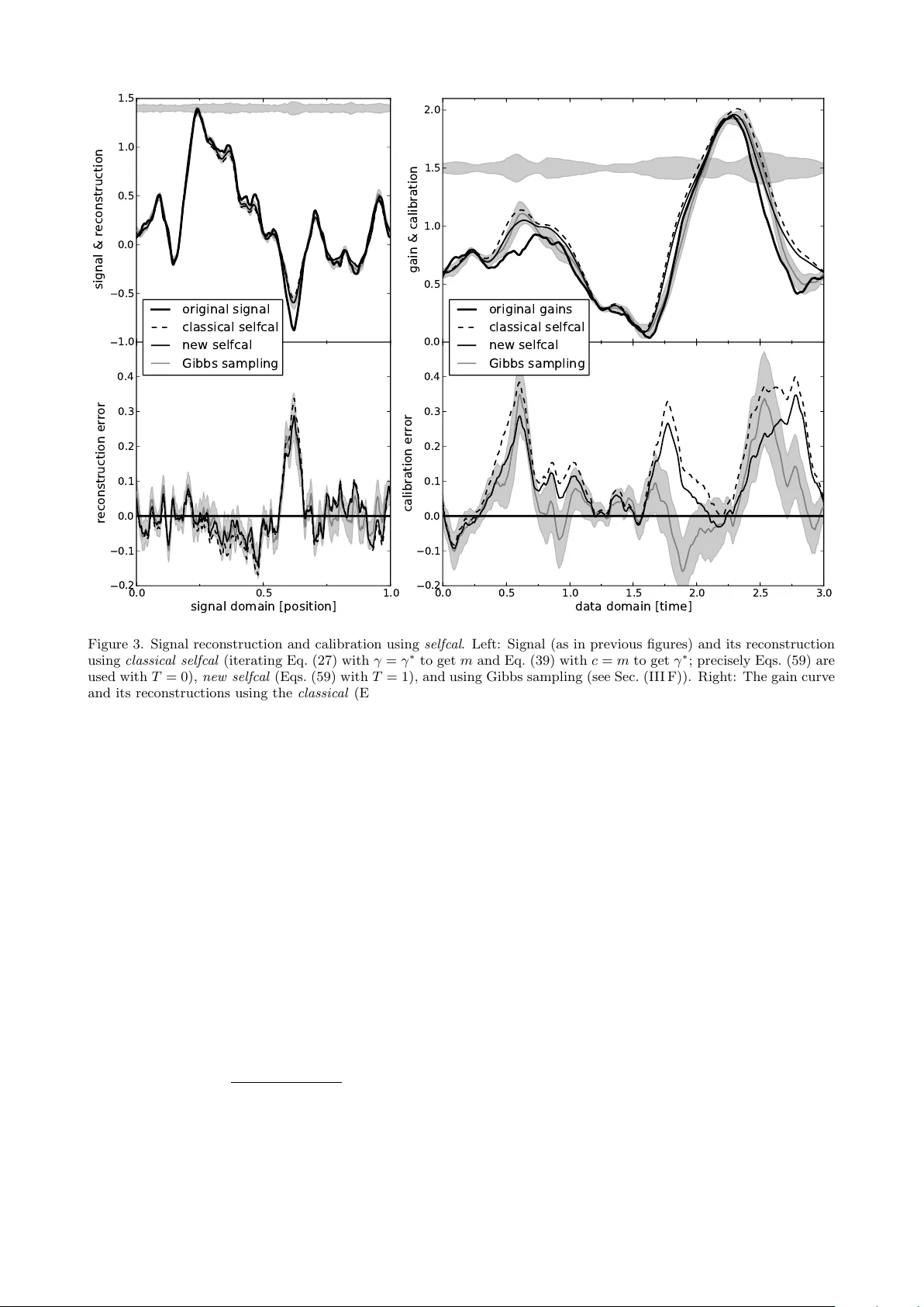
Impro ving self-calibration T orsten A. Enßlin, Henrik Junklewitz, Lars Winderling, Maksim Greiner, Marco Selig Max-Planck-Institut f¨ ur Astr ophysik, Karl-Schwarzschildstr. 1, 85748 Gar ching, Germany and Ludwig-Maximilians-Universit¨ at M¨ unchen, Geschwister-Schol l-Platz 1, 80539 Munich, Germany Resp onse calibration is the pro cess of inferring how m uc h the measured data dep end on the sig- nal one is in terested in. It is essen tial for any quantitativ e signal estimation on the basis of the data. Here, we inv estigate self-calibration methods for linear signal measurements and linear de- p endence of the resp onse on the calibration parameters. The common practice is to augmen t an external calibration solution using a known reference signal with an internal calibration on the un- kno wn measurement signal itself. Con temp orary self-calibration sc hemes try to ﬁnd a self-consisten t solution for signal and calibration b y exploiting redundancies in the measuremen ts. This can b e understo o d in terms of maximizing the joint probability of signal and calibration. Ho wev er, the full uncertain ty structure of this joint probability around its maximum is thereby not taken into accoun t b y these sc hemes. Therefore b etter sc hemes – in sense of minimal square error – can b e designed b y accounting for asymmetries in the uncertaint y of signal and calibration. W e argue that at least a systematic correction of the common self-calibration scheme should b e applied in many measuremen t situations in order to properly treat uncertain ties of the signal on whic h one calibrates. Otherwise the calibration solutions suﬀer from a systematic bias, whic h consequently distorts the signal reconstruction. F urthermore, we argue that non-parametric, signal-to-noise ﬁltered calibra- tion should pro vide more accurate reconstructions than the common bin a verages and pro vide a new, impro ved self-calibration scheme. W e illustrate our ﬁndings with a simplistic numerical example. P ACS n um b ers: 89.70.Eg, 11.10.-z, 02.50.Tt, 06.20.fb, 07.05.Kf Keywords: Information theory – Field theory – Inference metho ds – Standards and calibration – Data analysis: algorithms and implementation I. INTR ODUCTION A. Motiv ation An y measuremen t device needs a prop er calibra- tion, otherwise an accurate translation of the ra w mea- suremen t data into a common system of units is im- p ossible. Our abilit y to pro cess, combine, communi- cate, and draw conclusions from the results of mea- suremen ts dep ends critically on the ac hiev ed calibra- tion accuracy . The calibration problem is widespread across dif- feren t ﬁelds. Kno wing the ampliﬁer gain factors and detector eﬃciencies of ph ysical measuremen t appara- tuses is necessary to a nalyze their data. In astron- om y , the p oint spread function of a telescope obser- v ation migh t b e unkno wn, since it could dep end on v arying atmospheric inﬂuences. In analyzing sociolog- ical questionnaires, the reliability of p eople’s answ ers migh t diﬀer from topic to topic, but needs to b e taken in to accoun t. In all those cases, the measurement re- sp onse to the quan tity of interest, our signal, needs to b e known. This resp onse expresses how the data reacts (on av erage) to changes in the signal. Only if one knows the resp onse precisely , one can accurately reco ver the signal of interest correctly from data. The pro cess of the resp onse determination is called c ali- br ation , its result the c alibr ation solution , c alibr ation r e c onstruction , or just c alibr ation for brevity . Sev eral kinds of calibration uncertainties app ear in practice: oﬀsets (or additive noise), gain uncertain ties (or multiplicativ e noise), and nonlinearities (e.g. re- ceiv er saturation). This work deals with the ﬁrst tw o kinds of problems, multiplicativ e and additiv e noise. Noise denotes here an y inﬂuence of the data which is not due to the signal of interest, b e it sto chastic or just unkno wn in nature. Non-linear signal responses complicate the signal inference considerably . If the non-linearities are known, the generic insigh ts ab out the calibration of additiv e and m ultiplicativ e noise de- riv ed in this w ork still apply . The calibration of un- kno wn non-linearities is beyond the scop e of this pa- p er, though. The classical w a y to calibrate a measuremen t device is to apply it to a kno wn reference signal, the calibra- tor. The obtained instrument resp onse to this can then b e used to gauge the instrument and to in terpret the data obtained from measuring an unknown signal [1 – 6]. Ho wev er, in many measurement situations the re- sp onse dep ends strongly on time, lo cation, temp era- ture, energy , frequency , or other dimensions. A sim ul- taneous measurement of b oth calibrator and signal is often imp ossible. The external calibration needs then to b e extrap olated within the time (space, energy , ...) domain of the signal measuremen t. Extrapolation in time is only possible if the calibration exhibits suﬃ- cien t auto-correlation. This auto-correlation could be used to optimally ﬁlter out noise in the calibration so- lution. In practice, how ev er, usually only a veraging of the individual calibration solutions within suitably c hosen interv als is p erformed. An calibration obtained migh t b e further improv ed b y exploiting redundancies in the signal measuremen t. If the same asp ects of the signal are measured rep eat- edly , but the data sho w signiﬁcant deviations b etw een the individual measurements, this indicates a change in the instrument’s sensitivity . Thus, an external cal- ibration can often b e improv ed by an internal calibra- tion using the unkno wn signal itself as an additional source of calibration information. The usual in ternal calibration or self-calibration ( selfc al [7 – 14]) scheme pro ceeds as follows. A coarse external calibration is obtained and then applied to 2 the data to get a ﬁrst signal reconstruction. This sig- nal reconstruction is then used for a reﬁnemen t of the calibration, whic h in turn helps to further impro v e the signal reconstruction. The reconstruction and calibra- tion op erations are rep eated un til some desired con- v ergence criteria are met. It is, in general, unclear whether such a pro cedure con verges and whether the obtained solution is rea- sonable. There are selfc al schemes derived from min- imizing an ob jective function [6] and conv ergence can b e prov en for them. How ever, for empirically designed selfc al schemes, as used, e.g., in radio interferometry , suc h a pro of is often missing. It could well b e that only a self-consistent solution of an incorrect signal and an incorrect calibration is obtained, although the join t ﬁt to the data is perfect. This problem is of generic nature. If a measured da- tum dep ends on tw o unknowns, the signal and the in- strumen t sensitivity , these cannot unam biguously b e reconstructed. The additional presence of measure- men t noise makes this inference problem even harder. External calibration is essential, but often relies on the abilit y to extrapolate it in to domains in time or lo ca- tion, where – strictly sp eaking – it was not measured for. In this work, we show that the classical selfc al sc heme can b e understo o d as a join t maximization of the joint p osterior probability of signal and cali- bration giv en the data. This p osterior represents all a v ailable information on signal and calibration. A sta- ble ﬁx point of the selfc al scheme is a maxim um of this join t p osterior. It therefore represents the most likely com bination of signal and calibration, at least in some vicinit y of the ﬁx point. Ho wev er, such Maximum A Posteriori (MAP) es- timators are known to b e prone to ov er-ﬁtting the data. A posterior mean signal w ould b e optimal with resp ect to an exp ected square error norm [e.g. 15]. In case of a symmetric p osterior, mean and maximum co- incide and the MAP estimator is also optimal in this sense. Ho w ever, the presence of a nuisance param- eter, here being the unknown calibration, can turn an originally symmetric problem into a skew ed one. As a consequence, the maxim um of suc h a sk ewed, non-symmetric p osterior is systematically biased a wa y from the lo cation of the posterior mean [e.g. 16]. In- deed, we will show in this work that using the joint MAP estimator of signal and calibration, as the selfc al sc heme do es, implies a systematical bias with resp ect to the more optimal p osterior mean of signal and cal- ibration. B. Previous w ork The previous w ork on calibration is v ast, in par- ticular the mathematical-statistical literature. It may b e classiﬁed into whether it deals with univ ariate or m ultiv ariate calibration problems, concentrates on ex- ternal or in ternal calibration, and uses frequen tist or Ba yesian metho dologies. A review of v arious math- ematical treatments of external calibration (uni- and m ultiv arian t as w ell as frequen tistic and Bay esian) can b e found in [3]. External calibration means that an external, high- qualit y dataset is used to map out and reconstruct the resp onse of a measuremen t device. This could b e a single real function (univ ariate calibration, e.g. [1]) or a vector v alued function (m ultiv ariate calibra- tion, e.g. [2]). This calibrated resp onse is then used in the interpretation of the following measurements. The main challenge in external calibration is to con- struct a noise suppressing reconstruction op eration, whic h takes the often unknown noise v ariance prop- erly in to account. The function might be of para- metric form [1], or non-parametric estimators might b e used [4, 17]. It was realized that in many situ- ations a calibration obtained at some instant is not accurate for subsequen t measuremen ts, as the instru- men t migh t ha ve c hanged with time. An appropriate calibration transfer metho d should b e emplo y ed that tak es such uncertainties prop erly into accoun t [5]. In ternal calibration deals with the situation that an external calibration solution is not a v ailable, or is kno wn to b e inaccurate. F or example, the instrument resp onse might change on timescales comparable to the one needed to switc h the instrumen t to the cali- brator signal. This, for example, is a common problem in radio interferometry , where the rapidly changing Earth ionosphere can b e regarded as part of the tele- scop e optics. In suc h cases, the signal of in terest has to serv e as a calibration signal as w ell. The resulting selfc al sc hemes image the signal with an assumed cal- ibration, calibrate on this signal reconstruction, and rep eat these op erations un til conv ergence [7–14]. T o the knowledge of the authors, an information theoret- ical inv estigation is lacking ab out under which condi- tions this leads to reliable results, and when it fails, al- though practitioners certainly hav e developed a go o d in tuition on this. A rigorous information theoretical treatment of the problem of unknown calibration should b e build on the calibration marginalized lik eliho o d, since it con- tains all the av ailable information from the data and on the measurement pro cess. F or a measuremen t with Gaussian noise, linear resp onse, a nd linear calibration uncertain ties with a Gaussian distribution of known co v ariance this marginal likelihoo d can b e calculated analytically [18] and is repro duced here in Eq. (43). This likelihoo d is a Gaussian probability densit y in the data, with a signal dep endent cov ariance. Thus, the resulting signal p osterior is v ery non-Gaussian. If the mean of this signal p osterior can b e calculated, all the a v ailable internal calibration information is taken im- plicitly into account, and there is no need for a deter- mination of the calibration. In case of non-parametric measuremen t and calibration problems, the dimen- sionalit y of the problem is, how ever, often to o large (virtually unbound) for the usual Monte-Carlo meth- o ds to sample the p osterior. T o tac kle such and other problems information ﬁeld theory [15, 19, 20] was de- v elop ed. This exploits the mathematical and concep- tual similarities of the non-parametric inference prob- lem with statistical ﬁeld theories well-kno wn in math- ematical physics. F or example, the reconstruction of Gaussian random ﬁelds with unkno wn cov ariance, as 3 also needed for calibration, w as successfully treated in this framework [16, 17, 21–23]. F or the eﬀectiv e treatmen t of non-Gaussian p oste- riors the metho d of minimal Gibbs free energy [24] (a thermo dynamical incarnation of the v ariational Bay es approac h) has prov en to b e useful and was applied to the calibration marginalized signal inference problem b y Ref. [25]. Ho wev er, due to the contriv ed structure of the marginal likelihoo d, relatively coarse appro xi- mations had to b e used there to get to analytical for- m ulas. F or this reason, a more pragmatic approach shall b e follow ed here in tac kling the internal calibra- tion problem. C. Structure of this w ork This work is organized as follows. In order to de- v elop an in tuitive understanding, we in v estigate an illustrativ e example from a frequentist and Ba yesian p ersp ective in Sec. I I. Then, we inv estigate in Sec. I I I the general theory of calibration of linear measure- men ts with partly unknown resp onse operators, in particular external calibration, classical selfc al , and a new, uncertaint y corrected selfc al schemes. These diﬀeren t approac hes are compared in Sec. IV via a n umerical example that is based on the illustrative example of Sec. I I. W e conclude in Sec. V with a sum- mary of our main ﬁndings and a brief p ersp ectiv e on what would b e required to dev elop a full theory of calibration. I I. ILLUSTRA TIVE EXAMPLE It is the goal of this work to improv e the present selfc al schemes suc h that the reconstructed signal is closer to the a p osteriori mean. It turns out that this is a problem of high mathematical complexit y ev en for linear resp onses. The most imp ortant correction w e ﬁnd can b e understo o d in tuitiv ely , though. F or this, w e ﬁrst turn to a simplistic example, which we inv es- tigate using a less formal language. A more general and rigorous treatmen t will b e given in Sec. II I, which is able to deal with the complex linear resp onses one can ﬁnd in practice, lik e conv olving telescope b eams etc. The illustrativ e example introduced here will b e sim ulated in Sec. IV and is also the basis of the ﬁgures in this article. A signal s should b e observed with an instrumen t that has a sensitivit y or gain g . In our illustrative example, which will b e replaced by a more general case later on, the instrument’s data, d = g s + n, (1) is further corrupted b y noise n . Here and in the fol- lo wing, any calibration oﬀset in the data is regarded as part of the noise n . Signal, noise, and gains should b e indep endent sto c hastic processes so that their joint probability sep- arates according to P ( n, g , s ) = P ( n ) P ( g ) P ( s ) . (2) A t this stage, the problem of signal and gain recon- struction is symmetrically degenerate, since w e kno w as muc h ab out the signal as about the gain giv en the data. Typically , the gain is not completely unkno wn, for example, the sign of the instrument gain is usually kno wn. F or deﬁniteness, let us assume it to b e posi- tiv e and actually g = 1 + γ , with 1 b eing the kno wn part of the gain and γ denoting the unkno wn part that w e need to calibrate. This could as well b e p ositive as negativ e with the same probability . W e will refer to an y estimate of γ as a c alibr ation . A. F requen tist p ersp ective In frequen tist data analysis, rep eated instances of the data are assumed to exist. These permit to p er- form data a v erages that can b e tailored tow ards sta- tistical a verages. W e adopt for a momen t this p er- sp ectiv e, since it allows us to highlight the essence of the calibration problem. If we would know the calibration, we could infer the signal by av eraging ov er the data in a w ay that a verages ov er noise realizations, h d i ( n | γ ,s ) = (1 + γ ) s + h n i ( n ) | {z } =0 . (3) Here, w e assumed the noise to ha v e a zero mean and denote av erages ov er the probability of a giv en b by h f ( a ) i ( a | b ) ≡ ˆ D a f ( a ) P ( a | b ) . (4) Here ´ D a denotes the phase space integral of a , at the momen t a ﬁnite dimensional in tegral like ´ dn, and later on also path-integrals ov er functional spaces. In case we do not know the calibration, we could still learn something about the signal, if w e are able to av erage ov er the data in a wa y that a verages o v er noise and calibration realizations. This reveals the signal, since h d i ( n,γ | s ) = (1 + h γ i ( γ ) | {z } =0 ) s + h n i ( n ) | {z } =0 = s. (5) This is less sensitiv e to the signal since we need more data to p erform our a veraging of t w o sto chastic pro cesses, noise and calibration. But the p oint we w ant to mak e is that the signal can b e estimated from a suitable linear data av erage, even without kno wing the precise calibration, since there is a known and p ositiv e part of the response of the data to the signal. Obtaining information on the unknown calibration γ , which w ould help us to get the signal more accu- rately , is more diﬃcult. If we w an t to perform an analogous av eraging to retriev e some information on γ , now ov er noise and signal realizations, we ﬁnd h d i ( n,s | γ ) = (1 + γ ) h s i ( s ) | {z } =0 + h n i ( n ) | {z } =0 = 0 , (6) while assuming a zero mean for the signal as w ell. Th us, at linear order in the data, there is no calibra- tion information av ailable. W e cannot pro ceed with- out some kno wledge of the signal since the resp onse 4 of the data to our calibration could as w ell be p osi- tiv e (for s > 0) as negative (for s < 0). F urthermore, whenev er the signal is close to z ero, the data resp ond only p o orly to the calibration. In selfc al we obtain some information on the signal from the data, e.g., by using only the kno wn part of the response, which then might b e used to analyze the data for a b etter guess on the calibration. This means the data ha v e to b e used at least twice (ﬁrst a rough signal reconstruction, then calibrating on this) and w e end up with a scheme that is at least quadratically in the data. Indeed, if we in vestigate av erages ov er squared data, h d 2 i ( n,s | γ ) = h s 2 i ( s ) (1 + γ ) 2 + h n 2 i ( n ) , (7) w e ﬁnd that this con tains terms that are directly sen- sitiv e to the calibration and therefore calibration in- formation is a v ailable. It should b e noted that the sensitivity of this squared data to the gains depends on the signal (and noise) v ariance, which we therefore would need to kno w. Any systematic error in its determination from data will lead to a systematic bias in the calibration. If such a biased calibration is used again for impro v- ing the signal v ariance in an attempt to iterativ ely impro ve the calibration solution, the bias is even in- creased. Without any external calibration constraints, the selfc al solution w ould easily drift far aw ay from an initially acceptable calibration. 1 Th us, a strong, but self-consisten t bias can b e present in the results of selfc al . In practice, selfc al is rarely done using Eq. (7) as this requires to o muc h data with comparable calibra- tion co eﬃcients for getting reliable a verages to mea- sure the calibration from the data v ariance. More di- rect and more sensitive calibration metho ds are used, e.g. the men tioned iteration of reconstruction and cal- ibration steps. The selfc al instabilit y exists there as w ell, in a sligh tly more subtle form. F or the detailed information theoretical dev elopmen t and inv estigation of suc h metho ds, w e switc h no w to a Bay esian persp ec- tiv e. B. Ba yesian p ersp ective In probabilistic logic (see, e.g., Refs. [26 – 28]), only a single realization of a data set needs to b e a v ail- able. All reasoning has to be done conditional to these data and av erages o ver diﬀerent data realizations are not part of the resulting data analysis metho d. Prob- abilities express the strength of b elieve in a certain p ossibilit y conditionally that some other statement is assumed to b e true and not necessarily how often this p ossibilit y happens to be the case as in frequentist thinking. The data are regarded as a vector of v alues 1 This instability is well known in radioastronomical interfer- ometry . T o suppress it, it is common practice to apply selfc al only to either the phases of the complex gain coeﬃcients and to k eep the gain amplitudes ﬁxed or vice versa. d = ( d 1 , . . . , d n ) ∈ R n , n ∈ N , for whic h any datum d i could be the result of an unique, non-repro ducible measuremen t, as e.g. its gain g i = 1 + γ i probably nev er takes exactly the same v alue again. 2 The measurement equation of our illustrative exam- ple is still Eq. (1) if we read it as a v ector equation with comp onents d i = (1 + γ i ) s i + n i . (8) W e migh t wan t to calculate the signal av eraged ov er all unknowns, but conditioned to the data, m = h s i ( n,γ ,s | d ) , (9) since this is known (see, e.g., Ref. [15]) to minimize the exp ected square error h ( s − m ) 2 i ( n,γ ,s | d ) . (10) On linear order in the data, the optimal estimator of this mean is known to b e given b y (see e.g. [29]) m = h s d † i ( n,γ ,s ) h d d † i − 1 ( n,γ ,s ) d + O ( d 2 ) (11) with h s d † i ( n,γ ,s ) = h s s † i ( s ) | {z } ≡ S and (12) h d i d j i ( n,γ ,s ) = (1 + h γ i γ j i ( γ ) | {z } ≡ Γ ij ) S ij + h n i n j i ( n ) | {z } ≡ N ij , where the bar denotes complex conjugation. Here we deﬁned the matrices S = h s s † i ( s ) , Γ = h γ γ † i ( γ ) , and N = h n n † i ( n ) that express the a priori uncertaint y co v ariances in signal, calibration and noise, as well as the notation † for the transp ose of a vector (and its complex conjugate in case it is a complex num ber). This optimal linear estimator is known under many names, like Minimal Square Error (MSE) estimator, generalized Wiener ﬁlter [30], and others. Using matrix notation and deﬁning the comp onen t- wise matrix product ( S ∗ Γ) ij = S ij Γ ij (no summa- tion), we get m ≈ S [ S + S ∗ Γ + N ] − 1 | {z } F d (13) and ﬁnd that the reconstruction is a ﬁltered version of the data. The ﬁlter F reduces the v ariance since its “denominator” S + S ∗ Γ + N is sp ectrally 3 larger than the “n umerator” S . W e can w rite F < 1 (sp ectrally). As larger the noise v ariance N is with respect to the signal v ariance S , as stronger the down-w eighting of the data. F urther down-w eigh ting comes from the com bined signal and calibration v ariation S ∗ Γ. How- ev er, if N  S and Γ  1 (sp ectrally) the ﬁlter is 2 Repeated measurements or measurements with diﬀeren t in- struments can be combined into a single data vector b y simple concatenation of the individual data vectors. 3 Meaning that ξ † ( S + S ∗ Γ + N ) ξ > ξ † S ξ for ∀ ξ ∈ R n \ 0. 5 close to the identit y 1 and the signal estimate F d is nearly unﬁltered data. In any case, the expected co v ariance of this recon- struction, h mm † i ( n,s,γ ) = S [ S + S ∗ Γ + N ] − 1 S = F S < S, (14) is (sp ectrally) smaller than that of the signal, S. Using this linear data ﬁlter F , Eq. (13), is in general not a bad idea since it is a conserv ativ e approach to signal reconstruction under calibration uncertainties. It adds the impact of the calibration uncertaint y S ∗ Γ to the noise budget N of a generalized Wiener ﬁlter [30], which is then applied to the data. The disadv an- tage of this approach is that even in case the signal is so strong that the signal-to-noise ratio is excellent, S  N (spectrally), the calibration-noise co v ariance, S ∗ Γ, can still be substan tial as it increases with in- creasing signal strength. F or large calibration uncer- tain ties, b etter, and necessarily non-linear metho ds ha ve to b e used, since among all p ossible linear data ﬁlters, F is already the optimal one (in the sense of minimizing Eq. (10)). The optimal (non-linear) metho d can b e con- structed by rewriting (9) as m = ˆ D n ˆ D γ ˆ D s P ( n, γ , s | d ) s = ˆ D γ ˆ D s P ( γ , s | d ) s = ˆ D γ P ( γ | d ) ˆ D s P ( s | d, γ ) s = hh s i ( s | d,γ ) i ( γ | d ) . (15) Here, we hav e p erformed a noise marginalization 4 and hav e split P ( s, γ | d ) via the pro duct rule into P ( s | d, γ ) P ( γ | d ). The inner signal a verage h s i ( s | d,γ ) assumes the calibration to b e kno wn. How ev er, the outer a v erage goes o v er the unknown calibration while w eighting eac h p ossible calibration according to its p osterior probability given the data, P ( γ | d ). The inner signal av erage might in many situations b e well dealt with b y using the optimal linear estima- tor, h s i ( s | d,γ ) ≈ h s d † i ( n,s | γ ) h d d † i − 1 ( n,s | γ ) d = S R †  R S R † + N  − 1 | {z } ≡ W d, (16) where R = diag(1 + γ ) is the calibration dep en- den t resp onse matrix of our measurement. The pre- viously problematic signal suppression by the term S ∗ Γ in Eq. (13) b ecame more sp eciﬁc, since R S R † = S + S ∗ ( γ γ † ) and therefore Γ → γ γ † . W e therefore exp ect to obtain a higher ﬁdelity signal recov ery even when the subsequently applied calibration a veraging in Eq. (15) might smo oth out some of the features 4 This marginalization is trivial since the term P ( d | n, γ , s ) = δ ( d − (1 + γ ) s − n ) can b e obtained using Bayes theorem, which cancels the noise phase space integral ´ D n . presen t in h s i ( s | d,γ ) as the p osterior av erage h γ γ † i ( γ | d ) implies muc h less a veraging than the prior av erage Γ = h γ γ † i ( γ ) . It is common practice to use a single “b est” cali- bration solution γ ? , a so-called p oint estimate , instead of av eraging ov er all p ossible calibrations. Thus, im- plicitly P ( γ | d ) ≈ δ ( γ − γ ? ) is assumed. This is in- deed often a go o d approximation, as w e will argue in Sec. I I I G. The next order corrections that take in to accoun t the width of the distribution P ( γ | d ) are usu- ally small. An imp erfectly chosen γ ? has t ypically a larger impact on the reconstruction qualit y than these corrections and our fo cus should, therefore, b e on ho w to calibrate most reliably . Again, we regard the posterior mean as a goo d es- timate choose it as a starting p oint, γ ? = h γ i ( s,γ | d ) = hh γ i ( γ | d,s ) i ( s | d ) . (17) If we would kno w the signal close enough, calibra- tion would be simple, as we could ignore the outer av- eraging o ver P ( s | d ). W e would form signal subtracted data d 0 = d − s = γ s + n from which we could con- struct the optimal linear estimator of the calibration, γ ? ≈ h γ i ( γ | d 0 ,s ) ≈ h γ d 0† i ( n,γ | s ) h d 0 d 0† i − 1 ( n,γ | s ) d 0 = Γ R 0†  R 0 Γ R 0† + N  − 1 ( d − s ) , (18) with R 0 = diag( s ) b eing the resp onse of the data to the calibration parameters γ . Iterating the linear estimators for signal and cali- bration, (16) and (18) while assuming s = W d and γ = γ ? , is then a plausible selfc al scheme. It ig- nores, how ever, the uncertainties in signal reconstruc- tion and calibration and therefore migh t suﬀer from a bias similar to the one discussed b efore using frequen- tist argumen ts. In particular, the outer av eraging in Eq. (17) ov er P ( s | d ) is crucial. If we ignore for a momen t, for simplicity , the signal dependence of the “denominator” in Eq. (18) we see that our calibration estimator γ ? = h Γ R 0† [ . . . ] − 1 ( d − s ) i ( s | d ) ≈ O ( h s i ( s | d ) ) − O ( h s s † i ( s | d ) ) (19) requires the knowledge of the a p osteriori signal mean m = h s i ( s | d ) and v ariance h s s † i ( s | d ) since the tw o underlined “numerator” terms b oth contain the un- kno wn signal. In classical selfc al sc hemes h s s † i ( s | d ) is appro ximated b y m m † . The latter has, how ever, less v ariance than the former if m is a ﬁltered version of s as assumed here 5 . This means that a systematic bias is present in suc h schemes, as the O ( h s s † i ( s | d ) ) term is systematically underestimated by m m † leading to an ov erestimation of γ ? . The most imp ortant result of this w ork is to show ho w to correct for this bias. 5 See Eq. (14), which is v alid also here if w e set S ∗ Γ → 0 there. If m resulted from naive data av eraging, noise rem- nants might b e signiﬁcantly present and can lead to an ov er- estimation of the p osterior signal v ariance and therefore also to a systematically biased calibration. 6 Suc h a bias was not presen t in case of the signal es- timation using a p oin t estimator γ ? for the calibration (instead of the calibration av eraging). The diﬀerence lies in the fact that for the chosen illustrative data mo del, Eq. (8) (as well as for many realistic measure- men t situations), the symmetry of signal and gain as suggested by Eq. (1) is broken, since s v aries around zero and g around a kno wn non-zero v alue. Thus, signal estimators can b e built on a more reliably non- zero gain than calibration estimators, which hav e to exploit opp ortunistically any suﬃcien tly non-zero sig- nal ﬂuctuation suitable for calibration. I I I. THEOR Y OF CALIBRA TION A. Generic problem A more rigorous and more abstract treatmen t of the calibration problem should b e addressed now. The signal and data domain are not necessarily the same an ymore as signals liv e typically in con tinuous do- mains (time, p osition, or spectral spaces) and data sets are alwa ys ﬁnite. F or dealing with probabilities o ver spaces of contin uous functions (ﬁelds in physical language) we use the formalism of information ﬁeld theory [15, 19, 20]. A generic, linear resp onse that maps the signal into data domain will b e assumed. This co vers many real- istic measuremen t situations. Unknown prop erties of this response are to b e calibrated. The unknown sig- nal, calibration, and noise components are all assumed to ﬂuctuate around zero with known individual cov ari- ances, but no cross-correlations b etw een them. As we do not assume any higher order statistics of these com- p onen ts to b e known, the maximum entrop y criterion [27, 28, 31, 32] suggests we should model our a priori kno wledge states as Gaussian distributions. This do es not imply that our analysis is only v alid for Gaussian statistics. If signal, noise, or calibration follo w non- Gaussian distributions and those are known, the here deriv ed metho ds still pro duce sensible results. Just more eﬃcient metho ds migh t b e constructed that ex- ploit the additional statistical knowledge. W e assume that a signal s = ( s x ) x o ver some con- tin uous domain (parametrized by x ) was targeted by a linear measurement device that produced the ﬁnite dimensional data d = ( d i ) i with signal indep endent Gaussian noise n = ( n i ) i that includes also calibra- tion oﬀsets, d = R s + n. (20) The signal response R = R γ = ( R γ i x ) i x dep ends on the unknown calibration parameters γ = ( γ a ) a as w ell as on the signal and data domain coordi- nates, here x and i , b etw een which it translates via ( R γ s ) i = ´ dx R γ i x s x . This is the general form for an y linear signal resp onse. It not only embraces the illustrativ e example of the previous section, where R γ ix = δ ( i − x ) (1 + γ i ) , but also a conv olution with a calibration dep endent kernel, R γ ix = f ( i − x, γ ), F ourier-transformations, R γ kx = exp( ik x ), and more complex measurement situations. In general, the resp onse can dep end in a very com- plicated wa y on the unkno wn parameters γ . W e sup- p ose that a ﬁrst order T a ylor expansion captures the most relev an t dep endence, R γ = R 0 + X a γ a R γ ,γ a   γ =0 + O ( γ 2 ) , (21) with R 0 = R γ | γ =0 b eing the well calibrated part of the resp onse and R γ ,γ a = ∂ R γ /∂ γ a its linear dep en- dence on the calibration parameter. Thereby , w e ig- nore second order corrections in γ . T o hav e a compact notation, we deﬁne scalar pro d- ucts for the contin uous u -dimensional signal domain and its F ourier space as j † s = ˆ dx u j x s x = ˆ dk u (2 π ) u j k s k , (22) for the discrete data domain as n † d = X i n i d i , (23) and for the calibration parameter domain something analog to (23) or (22), dep ending on whether the cali- bration parameters form a discrete set or a con tin uous function. Discrete calibration parameters are instru- men t gains, since there are at most a ﬁnite num ber of parameters p er data v alue, so that the calibration do- main can b e mapp ed onto the data domain (the set of data indices). A contin uous set of calibration param- eters w ould b e the spatial sensitivity map of a tele- scop e, the so-called telescop e b eam, for which the do- main in which the calibration parameters reside (the sphere S 2 of directions in the telescop e frame) can of- ten b e mapp ed onto the signal domain (p ositions in the sky , also S 2 ).In order to hav e an illustrative case, w e assume further that the signal ob eys a priori a Gaussian distribution, P ( s ) = G ( s, S ) ≡ 1 | 2 π S | 1 / 2 exp  − 1 2 s † S − 1 s  , (24) with known cov ariance S =  s s †  ( s ) = ´ D s s s † P ( s ). This and other cov ariances are assumed here to b e kno wn either from similar previous measurements or on theoretical grounds. In practice, they might need to b e determined from the data themselves. This is of- ten well possible, as sho wn in Refs. [16, 21, 23, 24], and explained in Sec. II I C. The extension to non-Gaussian cases can be treated in future studies along the lines sk etched in Refs. [15, 16, 21, 24]. The noise co v ariance N =  n n †  ( n ) is assumed to b e known as well, leading to the likelihoo d P ( d | s, γ ) = P ( n = d − R γ s | s ) = G ( d − R γ s, N ) . (25) Lik eliho o d and prior can b e combined into the join t probability of data and signal, P ( d, s | γ ) = P ( d | s, γ ) P ( s | γ ) = P ( d | s, γ ) P ( s ) (see Eq. (2) for the last step), from whic h the signal p osterior for known calibration can be obtained via Ba y es theorem, P ( s | d, γ ) = P ( d, s | γ ) P ( d | γ ) = e −H ( d, s | γ ) Z ( d | γ ) . 7 0.0 0.5 1.0 signal domain [position] 1.0 0.5 0.0 0.5 1.0 1.5 signal & estimate s m + γ m + γ = 0 0.0 0.5 1.0 1.5 2.0 2.5 3.0 data domain [time] 1.0 0.5 0.0 0.5 1.0 1.5 2.0 2.5 3.0 data & signal response R γ s R γ = 0 s d Figure 1. Simulated signal (according to Eqs. (24) and (58)) and data realization from observing the signal three times (according to Eqs. (20), (25) and (57)). Left: Signal (line), its prior-free and therefore noisy estimation by Eq. (32) using the correct calibration ( γ , black dots), and no calibration ( γ = 0, gray triangles). Right: Data (dots), the signal resp onse R γ s (gray line, Eqs. (57) and (58)) and the resp onse in case of zero calibration, R γ =0 s (dashed, gray line, basically three rep etitions of the signal pattern). The diﬀerence betw een these t wo lines contains information on the calibration. The corresp onding gain curve is shown in Fig. (2). Here, we hav e introduced the information Hamilto- nian, H ( d, s | γ ) ≡ − log P ( d, s | γ ), and its partition function, Z ( d | γ ) ≡ ˆ D s e −H ( d, s | γ ) = ˆ D s P ( d, s | γ ) = P ( d | γ ) , (26) in order to exploit the mathematical and conceptual analogies of Ba y esian inference and thermo dynamics. B. Wiener ﬁlter Under these conditions, the optimal signal recon- struction for a given calibration γ is known to b e the Wiener ﬁlter (e.g., see Ref. [15]), m γ = h s i ( s | d γ ) = D γ j γ , (27) where D γ =  S − 1 + R γ † N − 1 R γ  − 1 , (28) j γ = R γ † N − 1 d, (29) are the information propagator (or Wiener v ariance) and information source, resp ectively [15]. This for- m ula is equiv alen t to the data space centric form ula for Wiener ﬁltering, see Eq. (16), we had argued to b e the optimal linear ﬁlter (minimizing Eq. (10)). The re- maining a p osteriori uncertaint y of the signal is giv en b y the Wiener v ariance,  ( s − m γ ) ( s − m γ ) †  ( s | d, γ ) = D γ . (30) Since the signal p osterior for kno wn calibration is a Gaussian (for this case comp osed of a Gaussian prior and likelihoo d, and a linear resp onse), it m ust b e P ( s | d, γ ) = G ( s − m γ , D γ ) , (31) as can also b e veriﬁed by a direct calculation. The often used so-called prior-fr e e or maximum lik eliho o d reconstruction can as w ell b e repro duced b y taking the limit of S → ∞ or S − 1 → 0, whic h remo ves an y prior con tribution to the ﬁlter formula, and in terpreting the matrix inv ersion in Eq. (28) as a pseudo-in verse 6 , so that m + γ = ( R γ † N − 1 R γ ) + R γ † N − 1 d. (32) This prior-free signal estimator is v ery noisy , as can b e seen from Fig. 1. There, a simulated signal, the resulting data, and the corresp onding prior-free sig- nal estimator are shown. The latter exhibits a lot of noise 7 compared to the reconstructions exploiting the kno wledge on co v ariances shown in Fig. 2. In the following, w e often suppress the γ - dep endence of R , D , j , m and other quantities for notational compactness, as we also do not note ex- plicitly that m is a function of the data d . 6 W e deﬁne the pseudo-inv erse of a Hermetian matrix A = P i a i a † i λ i with eigenv alues λ i and normalized eingenv ectors a i as A + = X i a i a † i ( λ − 1 i λ i 6 = 0 0 λ i = 0 . 7 This noise could b e reduced by binning, av eraging, or smo oth- ing. This requires that an a veraging length scale has to b e speciﬁed. The optimal a veraging length scale should be a trade oﬀ between suppressing noise and keeping signal fea- tures. How ev er, the Wiener ﬁlter, see Eq. (27), p erforms al- ready this a veraging in an optimal w ay (minimizing Eq. (10)) with an av eraging length that depends on the lo cal signal- response-to-noise ratio and therefore can v ary with p osition. W e therefore use in the following the Wiener ﬁlter metho d and regard binning and av eraging scheme applied in practice as approximativ e realizations thereof. 8 1.0 0.5 0.0 0.5 1.0 1.5 signal & reconstruction 0.0 0.5 1.0 signal domain [position] 0.2 0.1 0.0 0.1 0.2 0.3 0.4 reconstruction error original signal external calib. known calib. no calibration 0.0 0.5 1.0 1.5 2.0 gain & calibration 0.0 0.5 1.0 1.5 2.0 2.5 3.0 data domain [time] 0.2 0.1 0.0 0.1 0.2 0.3 0.4 calibration error original gains external calib. known signal no calibration Figure 2. Signal reconstruction and calibration without selfc al . Left: Original signal (as in Fig. (1)), and signal recon- structions using only the external calibration data (according to Eq. (39) with external calibrator c at only four moments as describ ed in Sec. IV), the correct gains ( g = 1 + γ , Eq. (27)), and no calibration ( g = 1, γ = 0 in Eq. (27)). Right: Original gains (according to Eqs. (35) and (58)) and their calibration reconstruction using only the external calibration data (as on the right hand side), calibrating on the correct signal (Eq. (39) with c = s ), and assuming no calibration ( g = 1, γ = 0). The gra y areas in the left and right panels sho w the one sigma p osterior uncertain ties of the signal and calibration reconstructions using the correct calibration and signal, respectively . These are the accuracies of the b est achiev able reconstructions and show that recov ering the calibration accurately is more diﬃcult than recov ering the signal. In the top panels these uncertainties are shown twice, once around the signal/calibration reconstructions and once at an arbitrary lo cation for b etter visual insp ection of their structures. C. P ow er sp ectrum estimation A problem in setting up the Wiener ﬁlter is of- ten that the signal and noise co v ariances are not kno wn precisely or migh t even b e completely un- kno wn. Thus, these need to b e inferred from the same data used for imaging. The prop er wa y is to form u- late h yp er-priors on these sp ectra, and to solve the com bined problem of simultaneous signal and sp ectra reco very . A suitable, how ev er numerically exp ensive metho d for this is Gibbs sampling [33, 34], here intro- duced in Sec. I I I F. An approximativ e, but numerically cheaper ap- proac h of iteratively analyzing a reconstruction for its cov ariance and using this cov ariance in improv ed reconstructions was developed in [16, 21, 23, 24]. The basic idea works for a statistical stationary sig- nal, for which the signal cov ariance is diagonal in F ourier space, with the p ow er sp ectrum P s ( k ) = h| s k | 2 i ( s ) on the diagonal (here, quan tities with the index k denote F ourier transformed quantities like s k = ´ dx s x exp( ik x )). In case of a Jeﬀreys prior on the p ow er sp ectra, a uniform distribution on loga- rithmic scale, the form ula to get a p oint estimate for the sp ectrum is P s ( k ) ≈ | m k | 2 + D kk , (33) where D kk corrects for the missing v ariance in the Wiener ﬁlter reconstruction m . Eq. (27) for m , Eq. (28) for D , and Eq. (33) for P s ( k ) hav e to b e iter- ated un til conv ergence. The accuracy of this sp ec- tral estimate can b e improv ed by a veraging F ourier mo des with similar spectrum and b y exploiting a v ail- able prior information on the spectral v alues and their smo othness as a function of w a vev ector [23, 35]. The metho d can even b e extended to estimate simultane- ously the signal and noise cov ariance [21] and b e com- bined with non-linear signal estimators [24, 36, 37]. Th us, an unknown cov ariance can be dealt with in principle. In order to b e able to concentrate on the essen tials of the calibration problem, we assume in the 9 1.0 0.5 0.0 0.5 1.0 1.5 signal & reconstruction 0.0 0.5 1.0 signal domain [position] 0.2 0.1 0.0 0.1 0.2 0.3 0.4 reconstruction error original signal classical selfcal new selfcal Gibbs sampling 0.0 0.5 1.0 1.5 2.0 gain & calibration 0.0 0.5 1.0 1.5 2.0 2.5 3.0 data domain [time] 0.2 0.1 0.0 0.1 0.2 0.3 0.4 calibration error original gains classical selfcal new selfcal Gibbs sampling Figure 3. Signal reconstruction and calibration using selfc al . Left: Signal (as in previous ﬁgures) and its reconstruction using classic al selfc al (iterating Eq. (27) with γ = γ ∗ to get m and Eq. (39) with c = m to get γ ∗ ; precisely Eqs. (59) are used with T = 0), new selfc al (Eqs. (59) with T = 1), and using Gibbs sampling (see Sec. (I I I F)). Righ t: The gain curve and its reconstructions using the classic al (Eqs. (59) with T = 0) and the new selfc al (Eqs. (59) with T = 1) scheme as w ell as using Gibbs sampling (Sec. (I I I F)). The uncertaint y estimates of the Gibbs sampling are shown as gray bands in all panels. In the top panels it is sho wn t wice, once around the Gibbs sampling mean and once at an arbitrary lo cation for b etter visual insp ection of its structure. follo wing known cov ariances as well as Gaussian prior distributions for signal, noise, and unknown calibra- tion parameters. Although w e sho wed that metho ds exist to obtain estimates of these cov ariances from the data them- selv es, we should in vestigate ho w sensitiv e a recon- struction is to inaccuracies in those estimates. F or this, we consider the sp ecial case of a signal and data space b eing identical, the resp onse the identit y ma- trix, and signal and noise b eing statistically homoge- neous pro cesses. In this case, their co v ariances are di- agonal in F ourier space, with the corresponding pow er sp ectra P s ( k ) and P n ( k ) on the diagonals. The Wiener ﬁlter in F ourier space is then m k = d k 1 + P n ( k ) /P s ( k ) . (34) Th us, high signal-to-noise (S/N) mo des with P n ( k ) /P s ( k )  1 are unmo diﬁed by the ﬁlter, m k ≈ d k , whereas low S/N mo des with P n ( k ) /P s ( k )  1 are strongly suppressed by the ﬁlter, m k → 0. Only for S/N ratios around one, the precise v alue of the sp ectra matters. Over- or underestimation of the S/N ratio leads to to o muc h noise in the reconstruction or an unnecessary strong signal suppression, respectively . Ho wev er, this eﬀect is mainly relev ant for the mo des with a S/N around unity . Therefore, mo derate inac- curacies in the p ow er sp ectra or cov ariances lead only to a minor degradation of the reconstruction ﬁdelity [16]. This usually also holds for more complex mea- suremen t situations than used in this argumentation [38]. D. External calibration Someho w, the calibration parameters γ hav e to b e measured in order that Eq. (27) can b e used to de- termine the a p osteriori mean of the signal. The sim- plest strategy is to use an external calibrator signal as a known reference from which the calibration can b e determined. In case the calibration parameters are constant in time, they can b e determined using a kno wn calibra- tion signal c and then b e transferred to the measure- men t of interest. The calibrator c = ( c x ) x is just a sig- nal, which ideally is known b efore the measuremen t, 10 whic h is strong enough to hav e a signal resp onse R γ c dominating ov er the noise, and which is suﬃcien tly complex to prob e the relev ant calibration uncertain- ties. The last requirement means that the calibrator resp onse should depend on the calibration parameters suc h that ∂ R γ c/∂ γ a ≡ R γ ,γ a c is signiﬁcan tly non-zero for any relev an t γ a . F or the calibration parameters we assume here and in the follo wing a Gaussian, zero-centered prior 8 , P ( γ ) = G ( γ , Γ) , (35) with known uncertaint y cov ariance Γ = h γ γ † i ( γ ) . The knowledge on Γ can come from theoretical con- siderations, previous measuremen ts, or migh t b e ob- tained from the data themselv es. Prior and likeli- ho o d, Eq. (25), form the join t probability P ( d, γ | c ) = P ( d | γ , c ) P ( γ ) that con tains all a v ailable information on the calibration. In general, the calibration inference from this is a non-linear and non-trivial problem. In many cases, the MAP approximation provides a reasonable esti- mate for γ . This is obtained by minimizing the corre- sp onding Hamiltonian H ( d, γ | c ) = − log P ( d, γ | c ) = 1 2 γ † Γ γ + 1 2 ( d − R γ c ) † N − 1 ( d − R γ c ) +const . (36) The gradient of this Hamiltonian, ∂ H ( d, γ | c ) ∂ γ = Γ − 1 γ − c † R γ † ,γ N − 1 ( d − R c ) , (37) should then b e follow ed (downhill) until it is zero and the Hamiltonian minimal. Here  R γ ,γ  a ≡ R ,a ≡ ∂ R γ /∂ γ a denotes the deriv ative of the resp onse with resp ect to the calibration. It is apparent that the dis- crepancy of the data from the calibration signal re- sp onse, d − R γ c , driv es the calibration solution aw a y from the default v alue γ = 0 preferred b y the prior of the calibration, P ( γ ) = G ( γ , Γ). In case the calibration parameters enter only lin- early , R γ = B 0 + X a γ a B a , (38) with B 0 and B a kno wn and γ -indep endent, we ha v e R ,a = R γ ,γ a = B a and the minimum of the Hamilto- nian is at γ ? = ∆ h, with (39) ∆ − 1 ab = Γ − 1 ab + c † B a † N − 1 B b c , and h b = c † B b † N − 1  d − B 0 c  . 8 The mean can alw ays b e subtracted by a redeﬁnition of the calibration parameters. As it is known, it should b e part of the known part of the resp onse, whereas the calibration parameter should only aﬀect the unknown part. This MAPstimator for the calibration γ ? is actually also the calibration p osterior mean h γ i ( γ | d, c ) , since this particular p osterior is a Gaussian for which mean and maximum coincide. This Gaussian calibration p osterior is P ( γ | d, c ) = G ( γ − γ ? , ∆) , (40) with the uncertaint y cov ariance ∆ = h ( γ − γ ? ) ( γ − γ ? ) † i ( γ | d, c ) giv en in Eq. (39). In this speciﬁc linear calibration case, external cal- ibration is Wiener ﬁltering. This can b e seen b y com- paring Eq. (39) with the Wiener ﬁlter equations for the signal, Eqs. (27)-(28), while recognizing that the roles of the follo wing terms corresp ond to eac h other: γ ? ↔ m , Γ ↔ S , N ↔ N , B 0 c ↔ R , ∆ ↔ D , d − B 0 c ↔ d , and h ↔ j . There is, how ev er, an interesting diﬀerence. The signal information source j = R † N − 1 d ≈ R † N − 1 R s =  B 0 N − 1 B 0 + O ( γ )  s contains a calibration-indep enden t term, B 0 N − 1 B 0 s , whic h re- acts to s ev en when γ = 0, whereas the calibra- tion information source h a ≈ c † B a † N − 1  R − B 0  c = P b  c † B a † N − 1 B b c  γ b = P a Q ab γ b is a quadratic function of the calibration signal c , which v anishes for lo cations with v anishing c . The quadratic depen- dence of Q ab = c † B a † N − 1 B b c on the calibration sig- nal strength will b ecome imp ortant again later on, when we inv estigate selfc al , the attempt to calibrate on an unkno wn signal. E. Calibration binning It should be noted that the usage of an a priori calibration cov ariance Γ = h γ γ † i ( γ ) to suppress the calibration estimation noise is not standard practice. Instead, bin-a veraging and interpolation is often p e r- formed on χ 2 or maximum likelihoo d calibration esti- mators. There is, how ev er, no consensus on the question how to c ho ose the bin size and in terp olation sc heme. The optimal bin size should, on the one hand, b e suﬃ- cien tly large to av erage down the noise, and on the other hand, b e suﬃciently small in order not to iron out existing small scale (spatial or temp oral) v aria- tions in the gain parameters. Therefore, the optimal bin choice depends on the in terplay of exp ected cal- ibration v ariations as enco ded in Γ, the noise level N , and the strength of the calibrator signal in data space R γ c . Since all these elements are part of the MAP gain estimator, c.f. Eq. (37), that reduces to the Wiener ﬁlter solution for linear calibration problems, Eq. (39), we exp ect the latter to implement (nearly) an optimal av eraging and interpolation scheme. The optimal bin size could b e read of from this sc heme (it should b e of the order of the correlation length of ∆), or, even b etter, the binning and a v eraging b e replaced with the more accurate calibration solution given by Eq. (37) or Eq. (39). In the following, we use the un-binned, non- parametric Wiener ﬁlter solution since it is optimal or close to optimal. W e b elieve that binning schemes used in practice and c hosen with exp erience can come 11 suﬃcien tly close to the Wiener ﬁlter p erformance as that the diﬀerence do es not matter muc h for our discussion. When they matter, an adoption of the here prop osed non-parametric Wiener ﬁlter calibra- tion metho dology w ould b e b eneﬁcial and highly rec- ommended for the application. F. Gibbs sampling The signal and the calibration are the tw o un- kno wns. Their join t p osterior probability distribu- tion P ( s, γ | d ) can b e prob ed via Gibbs sampling in case it is p ossible to draw samples from P ( s | d, γ ) and P ( γ | d, s ) [34, 39, 40]. These are Gaussian distribu- tions in our case, given b y Eqs. (31) and (40) (with c = s ), resp ectively , from which it is w ell possible to dra w samples. The Gibbs sampling pro cedure is then to up date a combined signal and calibration probe p ( i ) = ( s ( i ) , γ ( i ) ) → p ( i +1) = ( s ( i +1) , γ ( i +1) ) via s ( i +1) ← - P ( s ( i +1) | d, γ ( i ) ) , γ ( i +1) ← - P ( γ ( i +1) | d, s ( i +1) ) . (41) If this up dating is an ergo dic process for the combined p -space, as it is in our case of Gaussian probabilities, the sample distribution can be sho wn to conv erge to- w ards P ( s, γ | d ). Marginalization with respect to s or γ to obtain P ( γ | d ) and P ( s | d ), resp ectively , can b e obtained from the samples by forgetting the corresp onding marginal v ariable. Any posterior av erage, like h s i ( s | d ) , is given b y the corresp onding sample av erages. The Gibbs sampling provides therefore a route to calculate any desired estimate from the full p osterior, without in- v oking appro ximations, except for replacing the p os- terior in tegration by ﬁnite sampling and therefore get- ting some shot noise. Beating down this shot noise b y generating a large num b er of samples can b ecome computationally expensive, wh y it makes sense also to in vestigate analytical alternatives as we do in the fol- lo wing. Analytical inv estigations also provide deeper insigh t into the structure of the problem, which is less easily obtained from the sampling mac hinery . An yhow, we pro vide Gibbs sampling results as an optimal b enchmark for the diﬀerent selfc al sc hemes implemen ted in Sec. IV. G. Calibration marginalized imaging All relev an t information on the signal is con tained in the calibration marginalized p osterior, P ( s | d ) = ˆ D γ P ( s, γ | d ) . (42) In the case of linear calibration co eﬃcients, R γ = B 0 + P a γ a B a , see Eq. (38), the calibration marginal- ized likelihoo d, from which this posterior can b e con- structed, can be calculated analytically , P ( d | s ) = ˆ D γ P ( d | s, γ ) P ( γ ) = ˆ D γ G ( d − R γ s, N ) G ( γ , Γ) (43) = G d − B 0 s, N + X ab B a s Γ ab s † B b † ! . This result can b e found in Ref. [18]. 9 The resulting p osterior P ( s | d ) = P ( d | s ) P ( s ) / P ( d ) is non-Gaussian, as the signal ﬁeld appears as part of the calibration marginalized eﬀective noise, N + P ab B a s Γ ab s † B b † . Ideally , the mean of this signal p osterior is calculated since this gives the optimal sig- nal estimate. Ho wev er, integrating ov er this non-Gaussian func- tion is often infeasible. The quadratic dep endence of the eﬀective noise on the unknown signal inhibits that this can b e calculated via a simple Gaussian in- tegration. In high-dimensional settings, Mon te-Carlo metho ds used to estimate phase space integrals might b ecome to o exp ensive. In such cases, appro ximative strategies are needed. One is to use the MAP estima- tor for this p osterior. How ever, due to the sk ewness of the distribution, this can b e exp ected to give biased results. It is b etter to c haracterize the calibration p os- terior P ( γ | d ) by its mean γ ? and uncertaint y cov ari- ance ∆ and to use them to construct an appro ximative signal estimation. Let us assume we managed someho w to estimate the calibration as γ ? with some uncertaint y cov ariance ∆ and that w e can w ell approximate 10 P ( γ | d ) ≈ G ( γ − γ ? , ∆) . (44) F or a Gaussian signal ﬁeld with P ( s ) = G ( s, S ) we could simply use γ = γ ? in the Wiener ﬁlter formula, Eq. (27). Ho wev er, this is sub optimal if the calibra- tion uncertain ty is signiﬁcant. In that case, correction terms might b ecome imp ortant, whic h w e calculate no w to ﬁrst order in the calibration uncertaint y ∆. The optimal, calibration marginalized signal esti- 9 One can also simply calculate the ﬁrst tw o moments of the data giv en the signal av eraged o ver noise and calibration real- izations, ¯ d = h d i ( n,γ | s ) = B 0 s , h ( d − ¯ d ) ( d − ¯ d ) † i ( n,γ | s ) = N + P ab B a s Γ ab s † B b † , and realize that the calibration marginal- ized likelihoo d has to b e a Gaussian with this mean and v ari- ance, since b oth, noise and calibration uncertaint y , just add Gaussian v ariance to the data. 10 In the case of an external calibration of only linear calibration parameters, Eq. (38), we had shown in Eq. (40) this to b e an exact result. 12 mator is m = h s i ( s | d ) = D h s i ( s | d, γ ) E ( γ | d ) (45) = ˆ D γ P ( γ | d ) h s i ( s | d, γ ) ≈ ˆ D γ G ( γ − γ ? , ∆) m γ ≈ D ( j + 1 2 X ab [∆ ab ( j ,ba − M ,ba D j + 2 M ,b D M ,a D j − 2 M ,b D j ,a )] ) γ = γ ? . In the last step, we T aylor expanded m γ = D γ j γ up to second order in γ − γ ? , p erformed the Gaussian in tegration, exploited the Hermitian symmetry of ∆, suppressed in the notation the dependence of all cali- bration dep enden t terms on γ , and introduced further the notations M = R † N − 1 R, M ,a = R † ,γ a N − 1 R + R † N − 1 R ,γ a , M ,ab = R † ,γ a N − 1 R ,γ b + R † ,γ b N − 1 R ,γ a + R † ,γ a γ b N − 1 R + R † N − 1 R ,γ a γ b , j = R † N − 1 d, j ,a = R † ,γ a N − 1 d, and j ,ab = R † ,γ a γ b N − 1 d. (46) In case of only linear calibration parameters as in Eq. (38), R = B 0 + P a γ a B a , the deriv ativ es sim- plify to M ,a = B a † N − 1 R + R † N − 1 B a , (47) M ,ab = B a † N − 1 B b + B b † N − 1 B a , j ,a = B a † N − 1 d, and j ,ab = 0 . F rom Eq. (45) it b ecomes apparen t that the op- timal signal reconstruction in the presence of cali- bration uncertainties should con tain a correction to m ? = D γ ? j γ ? , which corrects for the p ossibility that certain structures in the data might well b e due to a miscalibration rather than b eing caused by real signal structures. Th us, the reconstruction will b e less prone to ov er-ﬁtting calibration errors. The expected level of this correction can, how ev er, b e exp ected to b e mo derate in typical situations. The individual correction terms in Eq. (45) can b e paired in to similar ones with opposite signs whic h partly , but not fully , balance each other. As a consequence, we exp ect only a mo derate net correction by them. F or the sake of clarit y of the following discussion, we will therefore neglect these corrections and only w ork with the lo west order signal estimator m ? = D γ ? j γ ? . The accuracy of this dep ends, how ev er, crucially on the qualit y of the calibration, which should therefore b e our fo cus. H. Self-calibration 1. Motivation In man y situations, only insuﬃcien t external cali- bration measuremen ts are a v ailable. In this case, the signal s of scientiﬁc interest has also to serv e as a cal- ibration signal. Some selfc al procedure has to b e ap- plied in which signal and calibration parameters hav e to b e determined simultaneously from the same data. F urthermore, the case of a p erfectly known exter- nal calibration is rarely met in practice. Usually , the calibration signal c was measured with another imp er- fect reference instrument as well as with the scientiﬁc instrumen t that is also used to observe the science signal s . W e can no w regard the combined measure- men ts ( c with reference instrumen t, c with scientiﬁc instrumen t, and s with scientiﬁc instrument) as a sin- gle measurement, with combined signals, resp onses, noises, and calibration parameter sets. In our mathematical description, w e can combine these individual measuremen ts into a single measure- men t of a m ulticomp onen t signal s 0 = ( c, s ) t b y a m ulticomp onent instrument delivering the combined data d 0 = ( d r c , d s c , d s s ) t . Here, the data d r c result from the measurement of the calibration signal c with the reference instrument r, the data d s c from the calibra- tion measuremen t of c with the scien tiﬁc instrumen t s, and data d s s from the science signal s measurement with the scien tiﬁc instrument s. The com bined mea- suremen t equation reads   d r c d s c d s s   =   R r c 0 R s c 0 0 R s s    c s  +   n r c n s c n s s   or d 0 = R 0 s 0 + n 0 , with the com bined noise v ector n 0 , and the combined resp onse R 0 of the three original measurements. In order that the calibration measuremen t provides an y b eneﬁt, the calibration parameters of the last t w o measuremen ts with the scientiﬁc instrument need to b e identical or at least suﬃciently correlated with each other. Since for this combined measurement no external calibration exists (we hav e incorp orated all external measuremen ts), it should as well be reconstructed with a selfc al scheme. 2. Pr actic e Selfc al usually consists of rep eatedly reconstructing the signal, assuming a calibration to b e correct, and determining the calibration, while assuming the sig- nal to be giv en. These steps are rep eated un til signal and calibration estimates hav e con verged suﬃciently . Ho wev er, a pro of that this conv erges and the meaning of the ﬁx p oint seem are often missing in the selfc al literature. Using simultaneously MAP estimators for the signal inference and the calibration actually means that the join t p osterior of signal and calibration parameters is extremized in b oth unknowns. This is equiv alen t to 13 the minimum of the information Hamiltonian, H ( d, γ , s ) = − log P ( d, γ , s ) = 1 2 ( d − R γ s ) † N − 1 ( d − R γ s ) + 1 2 γ † Γ γ + 1 2 s † S − 1 s + const , (48) whic h is as given by 0 = ∂ H ( d, γ , s ) ∂ s = D − 1 s − j     γ and (49) 0 = ∂ H ( d, γ , s ) ∂ γ = Γ − 1 γ − s † R † ,γ N − 1 ( d − R s ) . The resulting form ula are identical to the Wiener ﬁlter signal reconstruction, Eq. (27), and the calibration on this signal, Eq. (37). Thus, the joint MAP selfc al sc heme is equiv alen t or at least similar to the usual practice of iterating signal and calibration estimation. It has b een noticed, e.g. b y Ref. [16], that using a joint MAP solution simultaneously for signal and n uisance parameters (here the unkno wn calibration, in [16] the unkno wn signal cov ariance) can b e sub- optimal. It is b etter to use the signal marginalized p osterior to determine the calibration parameters and then to use the resulting parameters in the signal re- construction. This appro ximation is also known under the term Empiric al Bayes [e.g., Ref. 41]. I. Signal marginalized calibration The signal marginalized Hamiltonian, H ( d, γ ) = − log ˆ D s P ( d, γ , s ) (50) = 1 2  γ † Γ − 1 γ − T r (log D ) − j † D j  + const , can be minimized with respect to γ to ﬁnd the MAP calibration solution γ ? . The gradient and Hessian of this Hamiltonian are ∂ H ( d, γ ) ∂ γ a =  Γ − 1 γ  a + 1 2 T r ( D M ,a ) − j † D j ,a + 1 2 j † D M ,a D j and (51) ∂ 2 H ( d, γ ) ∂ γ a ∂ γ b = Γ − 1 ab + 1 2 T r ( D M ,ab − D M ,a D M ,b ) + 1 2 j † D M ,ab D j + j † D M ,a D j ,b + j † D M ,b D j ,a − j † ,a D j ,b − j † D j ,ab − j † D M ,a D M ,b D j. (52) The Hessian can be used to construct an approxima- tiv e calibration uncertain ty co v ariance matrix via ∆ − 1 ab ≈ ∂ 2 H ( d, γ ) ∂ γ a ∂ γ b     γ = γ ? (53) so that a Gaussian appro ximation of the calibration p osterior, Eq. (44), as well as an calibration marginal- ized signal reconstruction, Eq. (45), can b e obtained. It is instructiv e, to compare the classical formula used for external calibration, Eq. (37), to the one of selfc al (51). F or this w e ha v e to iden tify m = m γ = D γ j γ in Eq. (51), which reads no w ∂ H ( d, γ ) ∂ γ a =  Γ − 1 γ  a + 1 2 T r ( D M ,a ) − m † R ,a N − 1 ( d − R m ) , (54) with c in Eq. (37). W e see that the only change is the additional term 1 2 T r ( D M ,a ), which ensures that the signal uncertain ty is taken in to accoun t in the calibra- tion. In case of only linear calibration parameters as in Eq. (38), R γ = B 0 + P a γ a B a , a nearly closed cali- bration formula can b e giv en, γ ? = ∆ 0 h, with (55) ∆ 0 − 1 ab = Γ − 1 ab + T r  m m † + D  B a † N − 1 B b  , and h b = m † B b † N − 1 d − T r  m m † + D  B 0 † N − 1 B b  . This formula is not exactly closed, since m = m γ ? and D = D γ ? are still calibration dep endent. How- ev er, iterations as performed usually in selfc al schemes should con verge to a ﬁx p oin t. In practice, one might prefer to use a gradient sc heme based on Eq. (54) rather than to iterate Eq. (55) since the latter con- tains nested matrix inv ersions that are n umerically exp ensiv e. The apparent calibration co v ariance ∆ 0 is also not exactly identical to ∆ obtained from the in verse Hes- sian, Eq. (52), since precisely the calibration depen- dence of m and D w ere ignored in the iden tiﬁcation of ∆ 0 . It should, how ev er, b e a useful appro ximation with low er computationally complexit y than Eq. (52). A comparison of the calibration formulas, Eqs. (39) and (55) while identifying c with m , rev eals the main eﬀect of the signal marginalization. This inserts an additional signal uncertaint y cov ariance D wherev er a term m m † app ears. As w e had seen in case of the external calibration, the quan tity determining ho w sensitiv e the calibration information h reacts to γ , Q ab = s † B a † N − 1 B b s = T r  s s † B a † N − 1 B b  in h a ≈ P b Q ab γ b (neglecting the noise impact), depends quadratically on the unknown signal s . Using m m † as an estimator for the quadratic signal s s † underes- timates the v ariance of the latter, since m is a ﬁltered v ersion of s with less p ow er. The correct a posteriori exp ectation v alue for s s † ,  s s †  ( s | d,γ ) = m m † + D, (56) con tains the signal uncertain t y cov ariance D in order to correct for this bias. This is therefore the appro- priate term to b e used in Q ab . The calibration propagator ∆ also gets a similar term Q ab = T r  B a † N − 1 B b  m m † + D  that ensures that a go o d guess for the signal v ariance is used in the term describing the calibration measurement pre- cision. This additional p ositiv e term due to the D correction in ∆ − 1 decreases ∆ and makes therefore the calibration reconstruction γ ? = ∆ h less reactiv e 14 to v ariations in the data. This prev ents an ov er- calibration on data features that might b e caused by noise. F urthermore, the new selfc al scheme corrects a systematic bias of classical selfc al to wards delivering higher calibration v alues 11 . W e therefore susp ect the signal marginalized calibration pro cedure to provide a more accurate calibration and signal reconstruction than the classical join t MAP calibration pro cedure. Whether this is indeed the case, w e inv estigate nu- merically . IV. NUMERICAL EXAMPLE A. Gain uncertain ties As an illustrative case to compare the p erformance of the diﬀerent calibration schemes we inv estigate a simple one-dimensional measuremen t problem with gain ﬂuctuations in the spirit of th e simplistic example of Sec. I I. A signal ﬁeld s = ( s x ) x o ver the p erio dic domain Ω = { x } x = [0 , 1) ⊂ R is observed u = 3 times by a scanning instrument. The instrumen t has a p erfect p oin t like resp onse at scanning location x t = t mo d 1 at time t but a time v arying gain g t = 1 + γ t . The instrumen t samples with a p erio d τ = 2 − 9 ≈ 2 · 10 − 3 so that the i th data p oint is at lo cation x iτ = ( iτ ) mo d 1. It is con venien t to regard the data as a func- tion of time (which is discrete with p erio d τ , so that t ∈ { 0 , τ , 2 τ , . . . u } ) and to exploit the fact that the spatial and temp oral co ordinates are well aligned (ex- cept that the temp oral domain is u times larger than the spatial domain). The resp onse operator R tx = (1 + γ t ) δ ( x − x t ) (57) is of the linear calibration parameter form R γ = B 0 + P a γ a B a , Eq. (38), with B 0 tx = δ xx t and B a tx = δ at δ xx t so that R tx,t 0 = ( R γ tx ) ,γ t 0 = δ tt 0 δ xx t and R tx,t 0 t 00 = ( R tx ) ,γ t 0 γ t 00 = 0. 12 The Gaussian signal, noise, and calibration co v ari- ances are assumed to b e kno wn and to b e desc rib ed b y p ow er sp ectra in F ourier space. In our concrete 11 This is v alid in the here discussed case in which the signal is obtained via noise suppressing ﬁltering, otherwise the bias could even b e opp osite in cases, in which noise remnants add spurious v ariance to the reconstruction. 12 As a consequence of this simple resp onse and noise structure while assuming white noise with N tt 0 = σ 2 n δ tt 0 , we get M xy = δ xy X t δ xx t (1 + γ t ) 2 σ − 2 n , M xy,t = 2 δ xy δ xx t (1 + γ t ) σ − 2 n , M xy,tt 0 = 2 δ xy δ xx t δ tt 0 σ − 2 n , j x = X t (1 + γ t ) δ xx t d t σ − 2 n , j x,t = δ xx t d t σ − 2 n , and j x,tt 0 = 0 . example, we use P s ( k ) = a s [1 + ( k/k s ) 2 ] 2 , P γ ( ω ) = a γ [1 + ( ω/ω γ ) 2 ] 2 , and P n ( ω ) = a n , (58) resp ectiv ely . W e express the amplitudes as a s = σ 2 s λ s , a γ = σ 2 γ τ γ u , and a n = σ 2 n τ n in terms of their re- sp ectiv e v ariances σ 2 s = h s 2 x i ( s ) , σ 2 γ = h γ 2 t i ( γ ) , and σ 2 n = h n 2 t i ( n ) and correlation lengths λ s = 4 /k s , τ γ = 4 /ω γ , and τ n = τ . W e choose σ s = 1, σ γ = 0 . 75, and σ n = 0 . 2 and correlation lengths λ s = 0 . 3 and τ γ = 1 . 5. This wa y , we ha ve a unit v ariance signal, a 75% calibration uncertaint y and 20% white noise p er measuremen t (in terms of typical signal strength). The noise is white, the signal short-correlated (with ab out 3 correlation regions within the signal domain Ω) and the gain correlates ov er a sligh tly larger region (a bit more than the size of the signal domain Ω). The gains are only slightly correlated b et ween subsequent passages ov er the same p osition ( τ γ = 1 . 5). An y systematic diﬀerence in the data resulting from iden tical signal p ositions should b e due to gain v aria- tions. A decent selfc al sc heme should b e able to ex- ploit this redundancy to estimate the gains and there- fore the signal. Ho wev er, a global degeneracy of the data with re- sp ect to its v ariations b eing caused by signal and gain v ariations can only partly b e brok en b y the three redundan t scans o ver the signal domain. The data d t ≈ (1 + γ t ) s x t only rep ort a product of signal and resp onse and one of those can b e traded of for the other. Therefore, a few external calibration measure- men ts are essen tial to break the degeneracy globally . T o ﬁx this degeneracy , we assume that four addi- tional external calibration measuremen ts of the gain v alue hav e b een p erformed at certain times t j ∈ { 0 , 0 . 75 , 1 . 5 , 2 . 25 } , with d 0 j = (1 + γ t j ) c + n 0 j b y mo- men tarily switching the observ ation to a strong cali- bration source with a kno wn strength of c = 4. W e assume that the noise during these calibration mea- suremen ts is as b efore, n 0 j ← - G ( n 0 j , σ 2 n ). 13 The selfc al equations become γ ? = ∆ h, with (59) ∆ − 1 tt 0 = Γ -1 tt 0 + δ tt 0   q t + c 2 X j δ tt j   σ − 2 n , h t =   d t m x t − q t + c 2 X j δ tt j d 0 j   σ − 2 n , and q t = m 2 x t + T D x t x t . Here we introduced the exp ected p osterior v ariance of the signal realization as constrained by the data, 13 F or mental and notational conv enience w e ignore that dur- ing the external calibration measurement usually no science signal data can b e taken by real instruments. How ev er, this idealization is inessential and has only a negligible impact on the results. 15 T able I. Reconstruction error of the diﬀeren t reconstruc- tion for the example shown in Figs. 1-3. reconstruction metho d ε s ε γ Wiener ﬁlter using kno wn gains/signal 0.037 0.056 exp ected uncertainties of abov e 0.040 0.063 Gibbs sampling 0.073 0.116 exp ected uncertaint y of ab ov e 0.042 0.076 no calibration, unit gains 0.110 0.533 only external calibration 0.081 a 0.246 classical selfc al 0.089 0.192 new selfc al 0.073 0.141 a In this particular realization of signal, gain, and data, despite the external calibration b eing relatively p o or it has coincidentally provided a b etter signal reconstruction than classical selfc al . q t = h s 2 x t i ( s | d,γ ) = m 2 x t + D x t x t . F urthermore we in- tro duced T as a parameter that switches b etw een clas- sical selfc al ( T = 0) and the new signal marginalized selfc al ( T = 1). B. Calibration comparison A simulated signal, gain, and resulting data real- ization using the ab ov e sp eciﬁcations, as well as their reconstructions using diﬀeren t information, assump- tions, and approximations can b e seen in Figs. 1, 2, and 3. These were generated using the generic signal inference framework NIFT Y 14 [42]. W e quan tify the signal and gain reconstructions in terms of their a v erage squared errors, ε 2 s = ( m − s ) † ( m − s ) and ε 2 γ = 1 u ( γ ? − γ ) † ( γ ? − γ ), resp ectively . Their expectation v alues, in case of known Gaussian statistics, are giv en by h ε 2 s i ( d,s | γ ) = ˆ 1 0 dx D xx and h ε 2 γ i ( d,γ | s ) = 1 3 ˆ 3 0 dt ∆ tt . (60) The b est results are of course obtained when signal or calibration are known. These Wiener ﬁlter solu- tions are optimal (dotted lines in Fig. 2) and their un- certain ty estimates are reliable (gray regions in Fig. 2). The worst signal reconstruction is the one obtained while assuming unit gains (thin gray lines in Fig. 2). Using only the four external calibration measuremen ts giv es slightly b etter results (dashed lines in Fig. 2). The classical selfc al pro vides more accurate calibra- tion (dashed lines in Fig. 3), which is further im- pro ved by the uncertaint y corrections included in the new selfc al scheme (solid lines in Fig. 3). The b est selfc al solutions are pro vided b y the Gibbs sampling. Despite some numerical noise in the results, whic h can only be suppressed by inv esting a large n umber of samples, these are optimal and therefore provide 14 T o b e found at www.mpa- garching.mpg.de/ift/nifty . a go o d b enchmark for comparison. The new selfc al sc heme ob viously do es not fully reach the accuracy of the Gibbs sampling. Nev ertheless, it is a signiﬁcan tly impro vemen t ov er the classic al selfc al as its solutions are visibly closer to the optimal Gibbs sampling re- sults. These n um b ers and also the b ottom panels of Fig. 3 sho w further that the uncertain ties in the calibration are systematically larger than those of the signal. This is due to the fact that the selfc al has to rely on the sig- nal b eing signiﬁcan tly non-zero, which is not the case for many lo cations, whereas the signal reconstruction is data driv en for all positions except some rare points where the gain g = 1 + γ happ ens to v anish. Since the signal uncertaint y correction of the cal- ibration remov ed a systematic bias of the classical sc heme, whic h had let to ov erestimated gain solutions, the corresp onding reconstructed signal sho ws more v ariation as the one without this correction. This is visible by careful insp ection of the top left panels of Fig. 3. V. CONCLUSIONS W e inv estigated the calibration problem of signal reconstruction from data. Although w e concentrated on simpliﬁed cases, approximating all uncertain ties in signal, calibration, and noise to b e Gaussian dis- tributed, we b elieve that the gained qualitativ e in- sigh ts are also v alid in man y other circumstances. In case a p erfect or suﬃcient external calibration measuremen t is missing, the signal to be measured has also to serv e as a calibrator. This is usually done b y selfc al sc hemes, which reconstruct the sig- nal assuming some calibration, calibrate on the re- constructed signal, and iterate this until con v ergence or other termination criteria are met. W e hav e shown that suc h selfc al schemes arise naturally from trying to maximize the joint p osterior of signal and calibra- tion. W e therefore demonstrated that any ﬁx p oint of such selfc al iterations must b e a maximum of this p osterior. There is, how ev er, no guarantee that the obtained maximum is a global one. The joint MAP estimator is not necessarily optimal in the sense of an minimal exp ected square error. Due to the in terw ov en coupling b etw een signal and calibra- tion in the data this maximum is indeed not optimal. In order to obtain impro ved signal and calibration sc hemes, w e w ork ed out the calibration marginalized signal p osterior and the signal marginalized calibra- tion p osterior and the resulting maximum a posteri- ori estimators. Both contain corrections terms taking in to account the remaining uncertain ties of calibration and signal, respectively . F or the canonical situation that the signal is a quan- tit y that v aries around zero, whereas the signal re- sp onse has a known non-zero part, we argue that the calibration corrections due to signal uncertainties are more essential than the signal reconstruction correc- tions due to calibration uncertainties. The reason is that in this case, the information source of the data on the unkno wn signal con tains a calibration indep endent 16 term, whereas the information source for the calibra- tion requires signal information. This is reﬂected b y the observ ation that the calibration uncertaint y cor- rections for the signal as given b y Eq. (45) con tain pairs of m utually nearly canceling terms. In con trast to this, the calibration correction for signal uncertain ties as giv en b y Eq. (55) is of a sys- tematic nature. It reduces, on a v erage and for p ositive kno wn part of the resp onse, the v alues of the inferred calibration solution. This leads to a more pronounced and thereb y more accurate signal reconstruction as more of the data v ariance can b e assigned to the sig- nal. W e ha ve illustrated this with a simplistic numer- ical example. The prop osed improv emen t of selfc al schemes should not b e regarded as the ultimate theory of cal- ibration. A num b er of appro ximations ha v e been in- corp orated in order to limit the computational com- plexit y . In particular the mutual dependence of signal and calibration uncertain ties are not fully taken in to accoun t and only the dominant inﬂuence of the un- certain ties on the p osterior means of signal and cal- ibration were calculated. A comparison with a n u- merically exp ensive, but asymptotically exact Gibbs sampling scheme shows that the corrections are indeed a go o d step in the right direction. How ever, they also sho w that there is still space for further improv emen ts. Th us, w e b elieve that these corrections can help to reﬁne the contemporary art of calibration and thereb y impro ve measuremen t results in man y areas of science and technology . Ac knowledgemen ts W e gratefully thank V anessa B¨ ohm, Sebastian Dorn, and Niels Op ermann, for discussions, feedback, and commen ts. The calculations w ere performed us- ing the generic signal inference framew ork NIFT Y to b e found at www.mpa- garching.mpg.de/ift/nifty [42]. [1] H. Sc heﬀ´ e, The Annals of Statistics , 1 (1973). [2] P . J. Bro wn, Journal of the Roy al Statistical So ciety . Series B (Metho dological) 44 , pp. 287 (1982). [3] C. Osb orne, International Statistical Review / Revue In ternationale de Statistique 59 , pp. 309 (1991). [4] M.-A. Gruet, Ann. Stat. 24 , 1474 (1996). [5] R. N. F eudale, N. A. W oo dy , H. T an, A. J. Myles, S. D. Brown, and J. F err´ e, Chemometrics and Intel- ligen t Lab oratory Systems 64 , 181 (2002). [6] N. Padmanabhan, D. J. Schlegel, D. P . Finkb einer, J. C. Barentine, M. R. Blanton, H. J. Brewington, J. E. Gunn, M. Harv anek, D. W. Hogg, ˇ Z. Ivezi ´ c, D. Johnston, S. M. Kent, S. J. Kleinman, G. R. Knapp, J. Krzesinski, D. Long, E. H. Neilsen, Jr., A. Nitta, C. Lo omis, R. H. Lupton, S. Row eis, S. A. Snedden, M. A. Strauss, and D. L. T uck er, ApJ 674 , 1217 (2008), astro-ph/0703454. [7] J. F. Jones, Journal of Spacecraft and Ro ck ets 4 , 554 (1967). [8] F. R. Sch w ab, in 1980 International Optic al Comput- ing Confer enc e I , Society of Photo-Optical Instrumen- tation Engineers (SPIE) Conference Series, V ol. 231, edited by W. T. Rho des (1980) pp. 18–25. [9] T. J. Cornw ell and P . N. Wilkinson, MNRAS 196 , 1067 (1981). [10] T. Cornw ell, in Synthesis Mapping , edited by A. R. Thompson and L. R. D’Addario (1982) p. 13. [11] T. J. P earson and A. C. S. Readhead, ARA&A 22 , 97 (1984). [12] R. D. Ekers, in Ser endipitous Disc overies in R adio Astr onomy , edited by K. I. Kellermann and B. Sheets (1984) p. 154. [13] J. E. No ordam and O. M. Smirnov, A&A 524 , A61 (2010), arXiv:1101.1745 [astro-ph.IM]. [14] A. Lannes and J.-L. Prieur, Astronomisc he Nac hrich ten 332 , 759 (2011). [15] T. A. Enßlin, M. F rommert, and F. S. Kitaura, Ph ys. Rev. D 80 , 105005 (2009), [16] T. A. Enßlin and M. F rommert, Phys. Rev. D 83 , 105014 (2011), arXiv:1002.2928 [astro-ph.IM]. [17] J. H. Davis, C. Bœhm, N. Opp ermann, T. Enßlin, and T. Lacroix, Phys. Rev. D 86 , 015027 (2012), arXiv:1203.6823 [hep-ph]. [18] S. L. Bridle, R. Crittenden, A. Melchiorri, M. P . Hob- son, R. Kneissl, and A. N. Lasenb y, MNRAS 335 , 1193 (2002), astro-ph/0112114. [19] J. C. Lemm, ArXiv Physics e-prin ts (1999), ph ysics/9912005. [20] T. Enßlin, in Americ an Institute of Physics Confer- enc e Series , American Institute of Ph ysics Conference Series, V ol. 1553, edited b y U. von T oussaint (2013) pp. 184–191, arXiv:1301.2556 [astro-ph.IM]. [21] N. Opp ermann, G. Robb ers, and T. A. Enßlin, Ph ys. Rev. E 84 , 041118 (2011), [astro-ph.IM]. [22] N. Opp ermann et al., A&A 542 , A93 (2012), arXiv:1111.6186 [astro-ph.GA]. [23] N. Opp ermann, M. Selig, M. R. Bell, and T. A. Enßlin, Phys. Rev. E 87 , 032136 (2013), arXiv:1210.6866 [astro-ph.IM]. [24] T. A. Enßlin and C. W eig, Phys. Rev. E 82 , 051112 (2010), arXiv:1004.2868 [astro-ph.IM]. [25] L. Winderling, On the The ory of Calibration , Master’s thesis, Ludwig-Maximilians-Universit¨ at M ¨ unc hen (2012). [26] R. T. Co x, American Journal of Ph ysics 31 , 66 (1963). [27] E. T. Jaynes, Pr ob ability The ory, by E. T. Jaynes and Edite d by G. Larry Br etthorst, pp. 758. ISBN 0521592712. Cambridge, UK: Cambridge University Pr ess, June 2003. , edited b y Bretthorst, G. L. (2003). [28] A. Catic ha, ArXiv e-prints (2008), [ph ysics.data-an]. [29] S. Zaroubi, Y. Hoﬀman, K. B. Fisher, and O. Lahav, ApJ 449 , 446 (1995), astro-ph/9410080. [30] N. Wiener, Extr ap olation, Interp olation, and Smooth- ing of Stationary Time Series (New Y ork: Wiley , 1949). [31] E. T. Jaynes, Physical Review 106 , 620 (1957). [32] E. T. Jaynes, in Pro c. IEEE, V olume 70, p. 939-952 (1982) pp. 939–952. [33] S. Geman and D. Geman, IEEE T ransactions on P at- tern Analysis and Machine Intelligence 6 , 721 (1984). [34] B. D. W andelt, D. L. Larson, and A. Laksh- minara yanan, Ph ys. Rev. D 70 , 083511 (2004), 17 arXiv:astro-ph/0310080. [35] T. A. Enßlin and M. F rommert, ArXiv e-prin ts (2010), [36] M. Selig and T. Enßlin, ArXiv e-prints (2013), arXiv:1311.1888 [astro-ph.IM]. [37] H. Junklewitz, M. R. Bell, M. Selig, and T. A. Enßlin, ArXiv e-prints (2013), [astro-ph.IM]. [38] N. Opp ermann, H. Junklewitz, G. Robb ers, M. R. Bell, T. A. Enßlin, A. Bonafede, R. Braun, J. C. Brown, T. E. Clarke, I. J. F eain, B. M. Gaensler, A. Hammond, L. Harv ey-Smith, G. Heald, M. Johnston-Hollitt, U. Klein, P . P . Kron b erg, S. A. Mao, N. M. McClure-Griﬃths, S. P . O’Sulliv an, L. Pratley , T. Robisha w, S. Roy, D. H. F. M. Sc hnitzeler, C. Sotomay or-Beltran, J. Stev ens, J. M. Stil, C. Sunstrum, A. T anna, A. R. T a ylor, and C. L. V an Eck, A&A 542 , A93 (2012), [astro-ph.GA]. [39] B. D. W andelt, ArXiv Astroph ysics e-prin ts (2004), arXiv:astro-ph/0401623. [40] J. Jasche, F. S. Kitaura, B. D. W andelt, and T. A. Enßlin, MNRAS 406 , 60 (2010), [astro-ph.CO]. [41] S. Petrone, J. Rousseau, and C. Scricciolo, ArXiv e-prin ts (2012), arXiv:1204.1470 [math.ST]. [42] M. Selig, M. R. Bell, H. Junklewitz, N. Opp er- mann, M. Reineck e, M. Greiner, C. P acha joa, and T. A. Enßlin, A&A 554 , A26 (2013), [astro-ph.IM].

Improving self-calibration

Original Paper

Comments & Academic Discussion

Leave a Comment

Original Paper

Related Papers

Comments & Academic Discussion

Leave a Comment