Hierarchical Reverberation Mapping

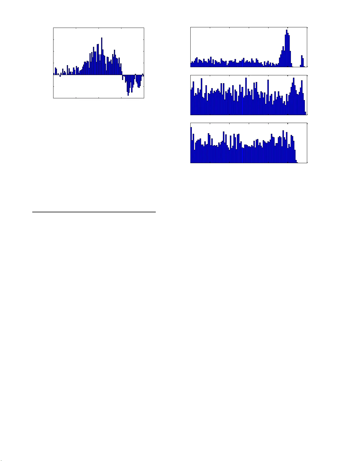
Mon. Not. R. Astron. So c. 000 , 000–000 (0000) Printed 21 July 2018 (MN L A T E X st yle file v2.2) Hierarc hical Rev erb eratio n Mappin g Brendon J. Brewer 1 ⋆ , T om M. Ellio tt 1 1 Dep artment of Statistics, The University of Auckland, Private Bag 920 19, Auckland 1142, New Ze aland T o b e submitted to MNRAS Letters ABSTRACT Reverberatio n mapping (RM) is a n important tec hnique in studies of activ e galactic nu clei (A GN). The key idea of RM is to measure the time la g τ betw een v ariations in the con tin uum emissio n fro m the accretion disc and subsequen t res po nse of the br o ad line region (BLR). The measurement of τ is t ypically used to estimate the physical size of the BLR and is co mbined with other mea surements to estimate the blac k ho le ma ss M BH . A ma jor difficult y with RM campaig ns is the large amount of data needed to measure τ . Recently , Fine et al. (20 12) intro duced a new appro ach to RM where the BLR light curv e is sparsely sampled, but this is counteracted b y observing a large sam- ple of AGN, rather than a single system. The r esults are combined to infer prop erties of the sample o f AGN . In this letter we implement this method using a hierarchical Bay esian mo del a nd contrast this with the results from the previous s ta ck ed cross - correla tion technique. W e find tha t our inference s are more pre c is e and allow for more straightforward interpretation than the stack ed cross-cor relation r esults. Key w ords: galaxies :a ctive — metho ds: data ana lysis 1 INTRO DUCTION Reverberation mapping (R M) is a key technique for the study of active galactic nuclei (AGN). The tec hnique is based on the temp oral fluctuations of the central contin- uum source, and t he subsequent response of the broad line region (BLR ) emission. The time d ela y b et w een the con tin- uum and th e broad line fl uctuations p ro vides an estimate of the size of the BLR, and can also b e u sed to estimate the blac k hole mass (P eterson 200 8). RM is a observ ationall y intensiv e, requiring observ a- tions of an AGN o v er a perio d of a few tens of days (Barth et al. 20 13). As a result, many au thors have stud ied the data analysis techniques in v olved in RM, and substantial adv ances hav e b een made in recent years . The data analysis metho ds introduced range from those that attempt to in- fer t he transfer function (the distribution of lags in a single ob ject, e.g. Krolik & Done 1995 ; Zu, Kochanek, & Peterso n 2011), th e vel ocity-resolved t ransfer function (Ben tz et al. 2010), or the physical structure of the B LR it- self (Pancoast, Brewer, & T reu 2011 ; Brewer et al. 2011; P ancoast et al. 2012; Li et al. 2013). There are many subtleties and challenges inv olv ed in reverberation mapping, th at we will ig nore for th e pur- p oses of t his letter. W e note tw o of them here for com- pleteness. Firstly , the mean lag ¯ τ = R τ Ψ( τ ) dτ , where Ψ( τ ) is the n ormalised transfer function, is not equ al to ⋆ b j . brewe r@auckland .ac.nz c times the mean radius of the BLR matter distribution, ¯ r = R p x 2 + y 2 + z 2 ρ ( x, y , z ) d 3 x . Second ly , the mean lag ¯ τ is not equiv alen t to the p eak of the cross-correlation function, except in the case of very narro w transfer func- tions. D irect physical mo delling of the BLR resolves these issues ( P ancoast, Brew er, & T reu 2011 ; Brewer et al. 2011; Li et al. 2013). Recently , Fine et al. (2012, 2013) in trod uced an inno- v ativ e approac h to reverberation mapping where the results from multiple AGN can b e combined to yield in ferences abou t the entire sample of AGN, d espite the fact that the constrain ts on any individual AGN are p oor. R ather than accurately measuring τ in a single ob ject, it is p ossible to roughly measure τ for a la rge num ber of ob jects (for exam- ple, by only measuring the BLR emission line flux at tw o ep ochs), and to infer properties ab out th e distribution of τ v alues in the sample of ob jects (and hence in a b roader p opulation, if the sample can b e considered representativ e). The data anal ysis approach of Fine et al. (2012) was based on an extension of t he traditional cross-correlatio n metho d to N separate ob jects. By “stac king” th e cross-correlation functions (CCFs) from the N ob jects in the sample, a p eak app ears which indicates a t ypical lag v alue in t he sample of AGN. Ho w eve r, this p eak is difficult to interpret. Sp ecif- ically , the width of th e p eak may b e influenced either by uncertaint y (du e to the sparse data) or du e to a wide range of lags being present in t he sample (i.e. th e sample of AGN is d iverse ). In t his letter, we revisit the idea of “stac k ed” re- c  0000 RAS 2 Br ewer an d El liott verberation mapp ing (i.e. using a sample of AGN with sparse data to infer something ab out the sample) from a Bay esian persp ective. W e d evelo p a Bay esian hierarchi- cal mo del ( Loredo 2004; Kelly 2007 ; H ogg, Myers, & Bo vy 2010; Shu et al. 2012; Loredo 2012 ; Brewer et al. 2013; Brew er, F orema n-Mack ey , & Hogg 2013). which allo ws us to calculate the p osterior distribution for hyp erparameters whic h describ e the typical lag, and the div ersit y of the lags. In Section 2 w e d iscuss the general p rinciples needed to com bine information from multiple po orly-measured ob- jects. In Section 3 we discuss the methods used to infer the lag τ using RM data for a single AG N. W e then demonstrate the t ec hnique on simulated data in Section 4, and conclude in Section 5. 2 COMBINING INF ERENCES ABOUT MUL TIPLE OBJECTS Consider a sample of N ob jects, ea ch of whic h has parame- ters θ i . If the i th ob ject is analysed on its own, the inference abou t its parameters θ i is described b y a p osterior distribu- tion p ( θ i | x i ) ∝ π ( θ i ) p ( x i | θ i ) (1) where π ( θ i ) is the p rior distribution and p ( x i | θ i ) is the like- lihoo d function. If N ob jects are analysed separately , in- ferences can b e made ab out th e diversit y of θ i across the sample. H o w ever, these inferences may b e incorrect du e to the implicit assumption that the prior for all of th e { θ i } is indep endent (Brew er et al. 2013). A hierarc hical mo del may b e used to o verco me this problem. In a hierarchica l model, the prior for the parameters { θ i } is created b y introd ucing hyp erparameters α suc h that the joint prior for α and the { θ i } is: p ( α, { θ i } ) = p ( α ) N Y i =1 p ( θ i | α ) (2) The implied prior on the { θ i } parameters is then p ( { θ i } ) = Z p ( α ) N Y i =1 p ( θ i | α ) dα (3) whic h may imply that the θ val ues are “clustered” aroun d some typical v alue. The p osterior dis tribution fo r { θ i } and the hyperparam- eters α given the data { x 1 , ..., x N } , is then p ( α, { θ i }|{ x i } ) ∝ p ( α ) p ( { θ i }| α ) p ( { x i }|{ θ i } , α ) (4) = p ( α ) N Y i =1 f ( θ i | α ) p ( x i | θ i ) (5) It is p ossible to consider th e d ata for all N ob jects as one big data set and infer the hyp erparameters α and the parameters of all ob jects { θ i } simultaneously . H o w ever, this can b e compu tationally prohibitive. In some circumstances it is tractable to analyse eac h ob ject’s data separately (using a common prior π ( θ i )) and then p ost-p rocess the results, reconstructing what the results of the h ierarc hical mo del w ould ha ve b een. In this letter w e use this latter approach. The marginal p osterior distribution for t he hyp erpa- rameters α is p ( α |{ x i } ) = Z p ( α, { θ i }|{ x i } ) d { θ i } (6) ∝ p ( α ) Z N Y i =1 f ( θ i | α ) p ( x i | θ i ) d N θ (7) ∝ p ( α ) N Y i =1 Z f ( θ i | α ) p ( x i | θ i ) dθ i (8) ∝ p ( α ) N Y i =1 Z f ( θ i | α ) π ( θ ) p ( x i | θ i ) π ( θ i ) dθ i (9) ∝ p ( α ) N Y i =1 E  f ( θ i | α ) π ( θ )  (10) where the exp ectation is taken with respect to the individ- ual ob ject p osterior of Equation 1 , and thus can b e esti- mated u sing p osterior samples from th e p osterior distribu- tions for th e individu al ob jects. This result enables us to reconstruct the posterior distribution for the hyp erparame- ters even though the individual ob ject inferences were made without the h ierarc hical structu re in the p rior. This is es- senti ally an importance sampling approximation to the full hierarc hical mo del. One drawbac k of this approac h is th at it implies an independ ent (non- hierarc hical) prior on any p er- ob ject nuisance parameters, which can sometimes adversely affect the results (e.g. Brewer et al. 2013). In Section 3 w e define a simple mod el for inferring the lag of a single AGN from sparse R M data. W e will u se Mark ov Chain Monte Carlo (MCMC) to pro duce p osterior samples for th e lags of th e N ob jects, which can then b e com bined using Equation 10 to yield th e p osterior distribu- tion for some hyp erparameters d escribing the distribution of lags in the sample. 3 THE SINGLE OBJ ECT MODEL If the contin uum light cu rve of an AGN is describ ed by a function y ( t ), th en the line ligh t curv e l ( t ) is given by l ( t ) = A Z τ Ψ( τ ) [ y ( t − τ ) + C ] dτ (11) where Ψ( τ ) is the transfer function (assumed t o b e nor- malised), and A and C are resp onse coefficients. The idea of reverberation mapping is to use noisy measuremen ts of y ( t ) and l ( t ) to infer the transfer function Ψ ( τ ) or a summary of it suc h as the mean lag ¯ τ = R τ Ψ( τ ) dτ . Throughout this letter we consider y ( t ) and l ( t ) in flux units, as opp osed to magnitudes, and consider ¯ τ as the definition of “the lag” of an AGN. The p osterior dis tribution fo r the lag ¯ τ of a single ob ject i may b e o btained b y fitting the follo wing mod el. W e assume, for simplicit y , that the transfer fun ction is un iform b etw een limits a and b , where b > a : Ψ( τ ) =  1 b − a , τ ∈ [ a, b ] 0 , otherwise (12) and our goal is to measure the mean lag: ¯ τ = Z τ Ψ( τ ) dτ (13) = 1 2 ( b − a ) . (14) c  0000 RAS, MNRAS 000 , 000–000 Hier ar c hic al R everb er ation Mapp ing 3 Note that inferring ¯ τ from the data req uires that w e marginalise ov er an infinite num b er of nuisance parame- ters describing the b ehaviour of y ( t ) at unobserved times (Pa ncoast, Brew er, & T reu 2011). The prior for the un - derlying time vari ation of th e continuum emission is a continuous autoregressiv e pro cess of order 1, or a CAR(1) mod el. These mod els hav e b een studied extensively for AGN v ariabili ty (e.g. Kelly , Bec h told, & Siemiginows k a 2009; Zu, Kochanek, & Peterson 2011; Zu et al. 2013). This marginalisati on can b e done either analytically or inside MCMC. W e used the latter app roac h for simplicit y . W e dis- cretised time using ten time bins p er d a y , an d h a ve a d is- crete contin uum light curve y = { y 1 , ..., y n } , in cluded in the mod el as a set of unkn o wn parameters. The prior for these parameters is: p ( y i | y i − 1 , m, k , β ) ∼ N  m + k ( y i − 1 − m ) , β 2  (15) for i > 2. This is the discrete AR(1) model from time series theory . m d escribes th e mean level of the contin uum light curve, β controls the size of the short-term fluctuations, and k contro ls the correlation t imescale ( the timescale itself is giv en b y L = − 1 / ln( k )). F or the likelihoo d (or sampling distribution, really the prior for the data given the parameters) we made the con- ven tional assumption of “Gaussian noise”: Y i ∼ N  y ( t y i ) , σ 2 y i  (16) L i ∼ N  l ( t l i ) , σ 2 l i  (17) W e used vag ue priors for the parameters of the single- ob ject model. In practice these could be made substan tially narro w er. W e c h ose a log-uniform prior for L (the AGN v ari- abilit y timescale) b etw een 0 . 1 and 10 5 days, a log-uniform prior for β (the size of th e short- term flu ctuations) b et w een 10 − 3 and 10 3 flux units, a Cauch y(0, 100) prior for m (the mean flux leve l of the AGN), a log-uniform p rior for b (the upp er limit of the transfer function) betw een 10 − 4 and 10 2 days, a uniform prior for a (th e low er limit of th e transfer function) betw een 0 and b , a log-uniform prior b etw een 10 − 3 and 10 3 for the resp onse co efficient A and a Ca uch y(0, 100) prior fo r the second resp onse parameter C . T o implement the MC MC for a single ob ject, w e implemented our model in the ST AN sampler (Hoffman & Gelman 2011) and Diffu sive Nested Sampling (Brew er, P´ artay , & Cs´ anyi 2011). Due to the large num ber of parameters, multiple mod es, and strong correlations in the p osterior distribut ion, w e found that Diffu siv e Nested Sampling was more effective than ST AN. Note t hat our single-ob ject model is already an impro vemen t ov er standard cross-correlatio n tec hniques and is similar to the approach used by Zu, Ko chanek, & P eterson (2011). 4 DEMONSTRA TION ON SIMULA TED DA T A T o test our h ierarc hical mo del, and compare it to the stac ked cross-correlatio n function, w e simula ted data from a sample of 100 AGN. W e assumed the continuum flux for eac h ob- ject fluctuates around a mean v alue m = 50 in arbitrary units. The v ariabilit y t imescales L were simulated from a very broad log-uniform distribution (i.e. a uniform distribu- tion for ln( L )) with a low er limit of 10 days and an u pp er limit of 1 , 000 days. The v ariabil ity amplitudes β were also sim ulated from a log-uniform dis tribution with lo w er li mit of 0 20 40 60 0 20 40 60 Flux 0 20 40 60 80 100 Time (days) 0 20 40 60 Contin uum Line Figure 1. Three simulated data set s, out of a total of 100. It i s difficult to inf er the lag ¯ τ f or an y of these ob jects (although there is some information av ailable). See Fi gure 3 for the ¯ τ p osterior distributions for these three data sets. 0.2 fl ux un its and an upp er limit of 1 fl ux u nit. This implies some ob jects are more v aria ble than others, as is t ypical in reverberation mapping. Eac h ob ject in the sample had its o wn transfer func- tion parameters. The upp er limit b of the transfer function w as sim ulated using a log-normal distribution with a me- dian val ue of 10 d a ys, and th e standard dev iation of ln( b ) w as 0.3. Given b , a wa s sim ulated from a uniform d istri- bution b etw een 0 and b . The resulting distribution of lags ¯ τ = ( a + b ) / 2 is v ery w ell approximated by a lognormal dis- tribution with a med ian of 7.4 d a ys and width (quantified by th e standard deviation of log 10 ( ¯ τ )) of 0.157 ( these tw o quantities are the ones w e will in fer u sing the hierarc hical mod el). The resp onse amplitudes A and C w ere set to 0.5 and 0 resp ectively , for all ob jects. N ote that the distribu- tion of the p arameters of the 100 ob jects is not the same as the p riors used w hen analysing t hem with the single-ob ject mod el. The measured data for each of the 100 AGN w as con- tinuum fl ux measurements, once p er da y , for 100 days. The standard deviation of the measuremen t noise is 1 flux unit (i.e. 2%). The line data is measured on only t w o da ys, with times selected from a uniform d istribution b etw een t = 50 and t = 100 days (i.e. corresp onding to th e latter h alf of the contin uum data). The flux of the line data is typically abou t h alf that of the contin uum data (since A = 0 . 5 for all ob jects), and t he measuremen t noise for the line data i s 0.25 flux units, or ab out 1%. S ee Figure 1 for three illustrative data sets from the sample. W e comput ed t he stacke d cross-correlation f unction for the 100 d ata sets. The cross-correlation function for a sin- gle ob ject is d efined as in Fine et al. (2012). F or a lag b in c  0000 RAS, MNRAS 000 , 000–000 4 Br ewer an d El liott 0 . 0 0 . 5 1 . 0 1 . 5 2 . 0 log 10 ( τ / (1 day)) − 400 − 200 0 200 400 600 800 Stack ed CCF Figure 2. T he stack ed cross-correlation function of the simulated data. A clear peak is seen around τ ≈ 10 days, but the stac ke d CCF has a large width. It is difficult to interpret the cause of this width, and to determine whether the w i dth is due to uncertain t y or diversity in the sample of AGN. These difficulties m otiv ate the hierarchica l Bay esi an model. b etw een τ and τ + δ the amount o f cross correlation is calcu- lated by looping o ver pairs of points (one selected from the conti nuum data set, and another from the line data set), and accumula ting mass when the lag b et w een the tw o p oints is b etw een τ and τ + δ . X ( τ ; δ ) = P N y i =1 P N l j =1 ( y i − ¯ y )  l j − ¯ l  1  ( t l j − t y i ) ∈ [ τ , τ + δ ]  P N y i =1 P N l j =1 1  ( t l j − t y i ) ∈ [ τ , τ + δ ]  (18) The den ominator is the num b er of pairs of p oints that fall within the lag range b eing considered, [ τ , τ + δ ], denoted n pair by Fine et al. (2012). The stack ed cross-correlation function for N ob jects is sum of the CCFs of the individu al ob jects. In Figure 2 , w e show th e stack ed CCF (on a log scal e) from our 100 simulated AGN data sets. There is a clear p eak around 10 days, and the full width at half maximum, while not strictly wel l defined, is roughly 0.25 d ex. As the d ata does not con tain meas urements at all p os- sible time lags, the stack ed CCF will alw a ys requ ire some smoothing. Here, the smooth ing is supplied by the choice of a bin width δ . The stack ed CCF has a substantial width. One weakness of the stack ed CCF meth od is t hat it is not clear wheth er this width is caused by real divers ity in the sample of AGN, or whether it is simply caused by the diffi- culty in measuring the lag ¯ τ of an ob ject with such sparse data. By contrast, the hierarc hical Bay esian approac h clearly separates these tw o concep ts. T o implement the hierarc hical Bay esian approach on the sim ulated data, we first used the single-ob ject model on eac h ob ject. The results for three ob jects (the same th ree ob jects shown in Figure 1 ) are plotted in Figure 3. Du e to the s parse data, there is a l arge a mount of uncertain t y ab out the v alue of ¯ τ for each system. Some ob jects do not al lo w an y real measuremen t of ¯ τ , but some do, as a result of fortuitous v ariabil ity of the con tin uum. Finally , w e combined th e results from the single-ob ject mod el into an inference ab out hyp erparameters µ and σ de- scribing the central v alue a nd th e divers ity of ¯ τ respectively , using the result of Equation 1. This req uires us to know the Posterior Probabilit y − 4 − 3 − 2 − 1 0 1 2 log 10 ( ¯ τ / (1 day)) Figure 3. Samples from the p osterior distri bution f or log 10 ( ¯ τ ) for three ob jects w hose data sets are shown in Figure 1. These posteriors were obtained by analysing each ob ject separately wi th the single-ob ject mo del. F or the first ob ject, there is a moderate “detect ion” of a l ag at ab out 10 days (although there is a small second mo de ab ov e 100 da ys, which can b e understoo d by in- specting the data in Figure 1). The second ob j ect’s lag w as not we ll constrained, and the third ob ject’s data only provided an upper limit on its lag. prior π ( ¯ τ ) implied by the simple-ob ject mo del, since we did not assign the prior d irectly to ¯ τ but indirectly through a and b . The prior for ¯ τ in the single-ob ject mo del is very wel l approximated by a log-uniform d istribution. Since lags ¯ τ are p ositiv e, our assumption for th e prior on ¯ τ giv en the h yp erparameters is a lognormal distribution with median µ and width (standard deviation of log 10 ( ¯ τ )) σ : log 10 ( ¯ τ ) ∼ N (log 10 ( µ ) , σ 2 ) (19) The joint p osterior d istribution for µ and σ , giv en the data from N = 100 AGN, is shown in Figure 4. The p rior for µ and σ was uniform inside th e rectangle show n, an d the p osterior distribution cov ers a m uch smal ler area, indi- cating that the data contained a lot of information ab out the hyperparameters. The true val ues used to generate t he sim ulated data are denoted by the star sym bol in Figure 4, and is typical of the posterior distribution, as it should b e. The marginal p osterior distribution for µ is show n in Figure 5 along w ith the p osterior predictiv e d istribution for the “next” ¯ τ v alue. The inference ab out µ can b e sum- marised as µ = 0 . 838 ± 0 . 047 (consistent with the known input v alue of 0 . 867 ≈ log 10 (7 . 4)), and t he p rediction ab out log 10 ( ¯ τ ) may b e summarised as log 10 ( ¯ τ ) = 0 . 838 ± 0 . 215. The Ba y esian approac h has clearly separated th e un cer- taint y ab out µ from the d iversi ty of the sample, describ ed by σ . Note t hat our metho d for combining indiv idual ob ject c  0000 RAS, MNRAS 000 , 000–000 Hier ar c hic al R everb er ation Mapp ing 5 − 2 . 0 − 1 . 5 − 1 . 0 − 0 . 5 0 . 0 0 . 5 1 . 0 1 . 5 2 . 0 µ 0 . 2 0 . 4 0 . 6 0 . 8 1 . 0 σ Figure 4. The joint p osterior distribution for µ and σ , hyper- parameters describing the distribution of ¯ τ v alues in the sample. The prior distribution was uniform ov er the ar ea shown. The true solution ( µ = 0 . 867 , σ = 0 . 157) is indicated by the white star symbol. µ = 0 . 867 corresp onds to a ty pical lag of 7.4 days. − 2 . 0 − 1 . 5 − 1 . 0 − 0 . 5 0 . 0 0 . 5 1 . 0 1 . 5 2 . 0 µ , log 10 ( ¯ τ / (1 day)) 0 2 4 6 8 10 Probability Density Posterior distribution for µ Predictive distribution for new ¯ τ Figure 5. The marginal posterior distribution for µ , the hyper- parameter descri bing the cen ter of the distribution for log 10 ( ¯ τ ), is plotted as the solid line. results into an inference ab out the p opulation (S ection 2 ) assumes t hat the hierarc hical prior app lies to only a single parameter (in our case ¯ τ ). If we incorp orate additional in- formation by using a hierarc hical prior for the other mo del parameters, allo wing u s to detect (for ex ample) th at all of the res p onse amplitudes A w ere e qual to 0.5, w e may be able to make more accurate inferences. How ev er, this w ould in- crease th e complexity of th e meth od and th e computational exp ense. 5 CONCLUSIONS Reverberation mapping campaigns are observ ationally in- tensive, yet p otentiall y very in formativ e. This has led to researc h into RM data analysis techniques, as wel l as less costly observing strategies. The recent approach of Fine et al. ( 2012) demonstrated th at it is p ossible to com- bine information from many sparsely-measured AGN and infer prop erties of the sample rather than insisting on accu- rate results ab out a p articular ob ject. In this letter w e exten ded the approac h of Fine et al. (2012) by implementing a Ba yesi an hierarc hical model for the data analysis. The main advan tage of this app roac h is a clear interpretation of the output, which is a p osterior distribution for hyp erparameters describing th e sample of AGN. W e demonstrated this approac h on a sim ulated data set consisting of 100 A GN with well-meas ured continuum light curves but sparsel y measured (t w o ep o chs per A GN) b road line light curves. F or the simula ted data set we were able to obtain an inference on µ , a hyp erparameter describing the typical val ue of the lag, to within 0.0 47 dex (1- σ uncer- taint y), whereas th e stac ked cross-correlation function had a FWHM of ∼ 0.25 dex. This is p ossible b ecause a sub set of the ob jects in th e sample will h a ve a measureable lag. W e hope this approac h will facilitate informative studies of samples of AGN. ACKNO WLEDGEMENT S It is a pleasure to thank T ommaso T reu, Ann a Pan- coast (U CSB), and Brandon Kelly (UCSB) for many use- ful conv ersations ab out reverberation mapp ing. The ST AN ( mc-stan.or g ) team provided helpful advice ab out the u se of their softw are. BJB is partially supp orted by the Mars- den F und (Roy al Society of New Zealand). W e are grateful to the referee, Stephen Fine, for his helpful commen ts. REFERENCES Barth A. J., et al., 2013, ApJ, 769, 128 Bentz M. C., et al., 2010, ApJ, 720, L46 Brew er B. J., et al., 2011, ApJ, 733, L33 Brew er B. J., P´ artay L. B., Cs´ anyi G., 2011, Statistics and Computing, 21 , 4, 649-656. Brew er B. J., F oreman-Mac key D ., Hogg D. W., 20 13, AJ, 146, 7 Brew er B . J., M arshall P . J., A uger M. W., T reu T., Dutton A. A ., Barnab` e M., 2013, arXiv, arXiv:13 10.5177 Fine S., et al., 201 3, MNRAS, 434, L16 Fine S., et al., 201 2, MNRAS, 427, 2701 Hogg D . W., Myers A. D., Bo v y J. , 2010, A pJ, 72 5, 2166 Kelly B. C., 2007, A pJ, 66 5, 1489 Kelly B. C., Bec htold J., Siemigino wsk a A., 2009, ApJ, 698, 895 Krolik J. H., Done C., 1995, ApJ, 440, 166 Li Y.-R., W ang J.-M., Ho L. C., Du P ., Bai J.-M., 2013, arXiv, Loredo T. J., 2004 , AIP Conference S eries, 73 5, 195 Loredo T. J., 2012 , arXiv, arXiv:1208. 3036 Hoffman M. D., Gelman A ., 20 11, arXiv, P ancoast A., Brewer B. J., T reu T., 2011, Ap J, 730, 139 P ancoast A., et al., 2012, Ap J, 754, 49 P eterson B. M., 2008, NewAR, 52, 240 Shu Y ., Bolton A. S., Schlege l D. J., Daws on K. S., W ake D. A., Brownstein J. R., Brinkmann J., W eave r B. A., 2012, A J, 14 3, 90 Zu Y., Ko chanek C. S ., Koz lo wski S., Udalski A., 2013, ApJ, 765, 106 Zu Y., Ko chanek C. S ., Peterson B. M., 2011, Ap J, 735, 80 c  0000 RAS, MNRAS 000 , 000–000