Group-Sparse Signal Denoising: Non-Convex Regularization, Convex Optimization
Convex optimization with sparsity-promoting convex regularization is a standard approach for estimating sparse signals in noise. In order to promote sparsity more strongly than convex regularization, it is also standard practice to employ non-convex …
Authors: Po-Yu Chen, Ivan W. Selesnick
LAST EDIT : DECEMBER 3, 2013 1 Group-Sparse Signal Denoising: Non-Con v e x Re gulariz ation, Con v e x Optimizati on Po-Y u Chen and Ivan W . Selesnick Abstract —Con ve x optimization with sparsity-promoting con- vex regularization is a standard approach for estimating sparse signals in n oise. In order t o p romo te sparsity more strongly than con v ex regularization, it is also standard practice to employ non - con v ex optimization. In this paper , we take a third approach. W e utilize a non-con vex r egularization term chose n such that the total cost fu nction (consisting of data consistency and regularization terms) is con vex . Theref or e, sparsity is more strongly promo ted than in the standard con v ex formulation, but wi thout sacrificing the attractive aspects of conv ex opti mization (u nique minimum, robust algorithms, etc.). W e use thi s i dea t o improv e the recently deve loped ‘ov erlapping group shrinkage’ (OGS) algorithm for the denoising of group-sparse signals. The algorithm is applied to the problem of speech enh ancement with fav orable results i n terms of both S NR and p erceptual quality . I . I N T R O D U C T I O N In th is work, we address the pr oblem of estimating a vector x from an observation y , y ( i ) = x ( i ) + w ( i ) , i ∈ Z N = { 0 , . . . , N − 1 } , (1) where w is additive white Gaussian noise (A WGN). W e assume that x is a gr oup-spar se vector . By gro up-sparse, we mean that large magn itude values o f x tend not to be isolate d. Rather , large magnitude values tend to f orm c lusters ( group s). Furthermo re, we do n ot assume th at the grou p loca tions are known, no r that the g roup boun daries a re known. In fact, we do not assume that the groups have well de fined bo undarie s. An example of such a vector ( in 2D) is the spectrog ram of a speech waveform. The spe ctrogram of a spee ch wa veform exhibits areas and ridges of large mag nitude, but n ot isolated large values. The method prop osed in this work will be demonstra ted on the prob lem of speech filtering. Con vex and non-conve x optimiza tion are both common practice fo r the estimation of sparse vecto rs from n oisy data [ 1 ]. In both cases one often seeks the solution x ∗ ∈ R N to the pr oblem x ∗ = arg min x n F ( x ) = 1 2 k y − x k 2 2 + λR ( x ) o where R ( x ) : R N → R is the regularization (or penalty ) term and λ > 0 . Con ve x for mulations a re advantageous in that a wealth o f con vex o ptimization th eory can be le ver - aged an d ro bust algo rithms with guara nteed conv ergence are av ailable [ 8 ]. On the other hand , non- con vex ap proaches are advantageous in that th ey u sually yield sparser so lutions for The authors are with the Department of Electric al and Computer Engi- neering , Polytec hnic Institute of Ne w Y ork Univ ersity , 6 Metrotech Center , Brooklyn, N Y 11201. Email: poyupaulc hen@gmail .com, selesi@ poly .edu, phone: 718 260-3416, fax: 718 260-3906. This research was support by the NSF under Grant No. CCF-1018020. a gi ven residu al energy . Howev er , non-c on vex formulatio ns are ge nerally mor e difficult to solve (due to subo ptimal local minima, initialization issues, etc.). Also, solutions produ ced by non-co n vex for mulations are generally discontinuou s f unctions of input da ta ( e.g., the discon tinuity o f the har d-thresho ld function ). Generally , conv ex appro aches are based on spar sity- promo ting conve x penalty fun ctions (e. g., th e ℓ 1 norm) , while non-co n vex appro aches are based on non-co n vex penalty f unc- tions (e.g., the ℓ p pseudo- norm with p < 1 [ 39 ], re- weighted ℓ 2 / ℓ 1 [ 10 ], [ 61 ] ). Oth er no n-conve x alg orithms seek sparse solutions directly (e.g., OMP [ 40 ], itera ti ve h ard thresholdin g [ 6 ], [ 25 ], [ 34 ], [ 51 ] , and greedy ℓ 1 [ 37 ]). In th is work , we take a different a pproach , p roposed by Blake and Zimmer man [ 5 ] an d by Nikolova [ 43 ]. Namely , the use of a no n-conve x non-smooth pena lty fu nction chosen such that the tota l cost fu nction F (consisting of da ta consistency and r egularization term s) is strictly conve x. This is possible “by balancing the positiv e secon d de riv ati ves in the [data consistency term] against th e n egati ve second deriv ati ves in the [pen alty] terms” [ 5 , pag e 1 32]. This idea has been f urther extended b y Nikolova e t al. [ 44 ], [ 46 ] –[ 48 ]. The con tribution o f this work relates to ( 1) the fo rmu- lation of the gr oup-spar se deno ising prob lem as a conv ex optimization problem albeit defined in terms of a non -conv ex penalty fun ction, an d (2) the derivation of a co mputation ally efficient iter ati ve algorithm that monoton ically red uces the cost fu nction value. W e utilize non- conv ex p enalty fu nctions (in fact, concave on the positiv e real line) with parametric forms; and we identify an in terval for the param eter that ensures the strict conve xity of the total cost function , F . As the total cost function is strictly con vex, the m inimizer is unique and can be o btained reliably using conv ex optimization technique s. The alg orithm we present is derived accord ing to the principle of majorization-m inimization (MM) [ 24 ]. The propo sed appro ach: 1) promotes sparsity more strongly than an y con vex penalty function can, 2) is translation in variant (due to group s in the p roposed method being fu lly overlapping), 3) is compu tationally e fficient ( O ( N ) per iteration) with decreasing cost f unction, and 4) requires no algo rithmic parameters (step-size, Lag range, etc.). W e dem onstrate be low th at the proposed app roach substan - tially improves u pon our e arlier work that consider ed only conv ex regularization [ 13 ]. 2 LAST EDIT: DECEM BER 3, 2013 A. Related W o rk The estima tion and reconstruc tion o f signals with gro up sparsity p roperties h as been addressed b y n umerou s authors. W e make a distinction betwe en two cases: non- overlapping group s [ 12 ], [ 21 ], [ 35 ], [ 36 ], [ 64 ] and overlapping gro ups [ 1 ]– [ 3 ], [ 14 ], [ 19 ], [ 23 ] , [ 32 ], [ 33 ], [ 41 ], [ 50 ] , [ 63 ]. The non - overlapping case is the easier case: whe n the grou ps are non-overlapp ing, ther e is a d ecouplin g of variables, which simplifies the o ptimization p roblem. When the group s are overlapping, the variables are coup led. In this case, it is com- mon to d efine auxiliary variables (e.g., thro ugh th e variable splitting techniqu e) and apply method s such as the alternatin g direction method of multiplier s (ADMM) [ 7 ]. Th is appr oach increases the num ber of variables (prop ortional to the gro up size) and hen ce increases memo ry usage an d data indexing . In previous work we describe the ‘overlapping grou p shrink age’ (OGS) algor ithm [ 13 ] fo r the overlappin g-grou p case that does not use auxiliary variables. The OGS algorith m exhibits fav or- able asymp totic conv ergence in co mparison with algorithm s that use au xiliary variables [ 13 , Fig. 5]. In co mparison with previous work on conve x optimizatio n for overlapping gro up sparsity , in cluding [ 13 ], the cu rrent work pro motes sp arsity more stro ngly . The curren t work extends the OGS algorith m to the case o f non-co n vex regularization, yet remains within the convex o ptimization f ramew ork. As note d above, the balancin g of th e data consistency term and the penalty term, so as to formulate a con vex pr oblem with a n on-convex p enalty term, was de scribed in Refs. [ 5 ], [ 43 ] and exten ded in [ 44 ], [ 4 6 ]–[ 48 ]. This approa ch was used to initialize a scheme named ‘graduated non-conv exity’ (GNC) in [ 5 ]. Th e go al of GNC is to minimize a no n-conve x fu nction F by min imizing a seq uence of fu nctions F k , k > 1 . The first one is a con vex approxim ation of F , and the subseq uent ones are non-co n vex an d pr ogressively similar to F . In order that the initial approxim ation of F be conve x, the penalty function mu st satisfy an eigen v alue co ndition [ 5 ]. A loo ser condition , which promotes sparsity more stro ngly , can b e expressed as a semidefinite pro gram (SDP), but this incu rs a higher compu tational co st [ 57 ]. In the m ethod described here , we use the same balancing idea as in GNC; however , o ur goal is to minimize a con vex function , not a n on-conve x o ne as in GNC. In p articular, we use the b alancing id ea to con struct a conv ex fu nction tha t m aximally p romotes spar sity , and we seek to subseq uently so lve this c on vex problem . W e n ote th at here our primary g oal is to captu re group sparsity behavior, which is not co nsidered in the GNC work. W e also no te that the computatio nally deman ding SDP arising in Ref. [ 57 ] does not arise in the curren t work. Th e algorithm developed here is compu tationally simp le. I I . P R E L I M I NA R I E S A. Notation W e will work with finite-leng th d iscrete sign als which we denote in lower case bold . The N -point signal x is written as x = [ x (0) , . . . , x ( N − 1)] ∈ R N . W e u se the n otation x i,K = [ x ( i ) , . . . , x ( i + K − 1 )] ∈ R K (2) to deno te the i -th group o f vector x of size K . W e consistently use K (a positive integer) to denote the gr oup size. At th e bound aries (i.e., for i < 0 and i > N − K ), some indice s of x i,K fall o utside Z N . W e take these values as zer o; i.e. , fo r i / ∈ Z N , we take x ( i ) = 0 . W e d enote the n on-negative real line a s R + := { x ∈ R : x > 0 } and the po siti ve real lin e as R ∗ + := { x ∈ R : x > 0 } . Given a fun ction f : R → R , the left-sided and right- sided d eriv ati ves of f at x are de noted f ′ ( x − ) an d f ′ ( x + ) , respectively . The notation A \ B d enotes set difference; i.e., A \ B = { a ∈ A : a / ∈ B } . B. P en alty Functio ns W e will m ake the following assumption s o n the penalty function , φ : R → R . 1) φ is co ntinuou s on R . 2) φ is twice differentiable on R \ { 0 } . 3) φ ( − x ) = φ ( x ) (symm etric) 4) φ ′ ( x ) > 0 , ∀ x > 0 (increa sing on R ∗ + ) 5) φ ′′ ( x ) 6 0 , ∀ x > 0 (con cav e on R ∗ + ) 6) φ ′ (0 + ) = 1 (u nit slope at zer o) 7) φ ′′ (0 + ) 6 φ ′′ ( x ) , ∀ x > 0 (maxim ally co ncave a t zero) W e will utilize p enalty function s parameterized by a scalar parameter, a > 0 . W e use the no tation φ ( x ; a ) to deno te th e parameteriz ed form . Examples o f param eterized penalty functions satisfying the assumptions above are the logar ithmic p enalty , φ log ( x ; a ) = 1 a log(1 + a | x | ) , (3) the arctang ent pe nalty [ 57 ], φ atan ( x ; a ) = 2 a √ 3 tan − 1 1 + 2 a | x | √ 3 − π 6 , (4) and the first order ratio nal fu nction [ 28 ] φ rat ( x ; a ) = | x | 1 + a | x | / 2 . (5) The ration al pen alty is defined for a > 0 . The log an d atan penalties are d efined for a > 0 . Note th at as a → 0 , th e three penalty fu nctions ap proach the absolu te value fun ction. They are illustrated in Fig. 1 . For later use, we record the value of the righ t-sided seco nd deriv ati ve of th e three penalty functions: φ ′′ log (0 + ; a ) = φ ′′ atan (0 + ; a ) = φ ′′ rat (0 + ; a ) = − a. (6) Note that the ℓ p pseudo- norm ( 0 < p < 1 ), i.e., φ ( x ) = | x | p , does n ot satisfy the above assumptions. It does n ot have unit slope at zer o nor can it be n ormalized or scaled to do so. 3 −20 −15 −10 −5 0 5 10 15 20 0 5 10 15 20 x Penalty functions, φ (x; a) with a = 0.2 abs log rat atan Fig. 1. Se vera l sparsity promoting penalty functions satisfying the assump- tions in Sec. II-B . C. Thres hold Functio ns Proximity operators are a fundam ental tool in efficient sparse signa l p rocessing [ 16 ], [ 17 ]. In the scalar case, proxim - ity opera tors are threshold ing/shrink age f unction derived using a conv ex penalty fu nction. I n th is work, we utilize n on-conve x penalty functio ns; howe ver , we can still define a th reshold function similar to the definitio n of a pro ximity operato r . The following prop osition is c losely r elated to L emma 3.1 in [ 42 ] and Theorem 3.3 in [ 45 ], b oth of wh ich an alyze the b ehavior of θ for non-smo oth, no t n ecessarily conve x, φ . Proposition 1. Define θ : R → R by θ ( y ) = ar g min x ∈ R n G ( x ) = 1 2 | y − x | 2 + λφ ( x ) o (7) where G : R → R , λ > 0 , and φ satisfies the assumptions in Sec. II-B . Suppose also th at G is strictly co n vex. If | y | 6 λ , then the unique min imizer of G is zero. That is, θ is a thr eshold function and λ is the th r eshold value. Pr o of: Th is is a special case of Prop osition 3 wherein θ is a mu lti variate thresho ld function , θ : R K → R K . Figure 2 illustrates threshold fu nctions corr espondin g to se veral penalty function s. W e use λ = 4 and a = 0 . 2 . Th e threshold fun ction corr espondin g to the abso lute value penalty function is called the soft threshold f unction [ 20 ]. Notice that, except fo r th e soft threshold fun ction, the th reshold f unctions approa ch the identity fu nction. T he atan thre shold fun ction approa ches identity the fastest. The fact that the soft threshold function redu ces large v alues by a constan t am ount is considered its deficiency . In the estimation of sparse signals in A WGN, this behavior results in a systematic under estimation (bias) of large magnitud e signal values [ 22 ]. Hence, threshold function s that are asymptotically unbiased are o ften pref erred to the sof t thresho ld func tion, and the penalty fu nctions fr om which they are derived promo te sparsity more strongly than the ℓ 1 norm [ 10 ], [ 11 ], [ 26 ], [ 27 ]. The atan p enalty fun ction is der i ved specifically fo r its fa vorable beh avior in th is regard [ 5 7 ]. As shown in Ref. [ 57 ], if φ satisfies the ab ove assumptio ns, then th e righ t-sided deriv ati ve of θ at the th reshold is given by θ ′ ( λ + ) = 1 1 + λφ ′′ (0 + ) . (8) 0 2 4 6 8 10 12 0 2 4 6 8 10 12 Threshold functions, θ atan rat log abs Fig. 2. Threshold functions deri v ed from the four penalty functions giv en in Sec. II-B ; three of which are non-con v ex. Hence, with param eters λ = 4 and a = 0 . 2 , we use ( 6 ) to find that θ ′ ( λ + ) = 5 fo r φ log , φ atan , and φ rat . Th at is, each of th ese thresho ld fu nctions in Fig. 2 have the same deriv ativ e at λ + , but they approac h the id entity at d ifferent rates. I I I . O G S W I T H N O N - C O N V E X R E G U L A R I Z AT I O N For de noising group- sparse signals in A WGN, we p ropose to minimize the cost functio n, F : R N → R , F ( x ) = 1 2 k y − x k 2 2 + λ X i ∈ Z φ ( k x i,K k 2 ; a ) (9) where φ is a (non -conve x) spar sity pr omoting penalty f unction satisfying th e assumptions in Sec. II-B , and λ > 0 . The gr oup size, K (a positive in teger), should be selected b ased on the size of the groups (clusters) arising in the data. This constitutes one’ s ‘prior knowledge’ regardin g the gr oup sparsity beh avior of the data and may need to be obta ined thr ough som e trial- and-err or . In o rder to lev erage convex optimizatio n princip les and av oid non-co n vex o ptimization issues (loc al m inima, sensi- ti vity to noise, etc.), we seek to restrict a so that F is strictly conve x. W e note that the min imization of F is not so straight fo rward. First, all th e variables a re coupled due to the overlapping group structure o f the regularization term. That is, each comp onent x ( i ) de pends on ev ery da ta sample y ( k ) (albeit the influence diminishes with distance | i − k | ). Secondly , F is not differentiable. In pa rticular, F is generally not d ifferentiable at the minimizer, x ∗ , du e to th e sp arsity of x ∗ induced by the regularizer . (The p enalty fu nction, φ , is non-d ifferentiable at zero ). For these rea sons, it is desirable that F be strictly co n vex. In the following, we add ress the qu estions: 1) For wh at values of a is F strictly conv ex? 2) When F is strictly conve x, how can the u nique mini- mizer, x ∗ , be efficiently comp uted? 4 LAST EDIT: DECEM BER 3, 2013 First, we make a few remark s. If K = 1 , then F simplifies to F ( x ) = X i h 1 2 | y ( i ) − x ( i ) | 2 + λφ ( x ( i ); a ) i , ( 10) the co mponen ts x ( i ) are not cou pled, and the minimization o f F amounts to comp onent-wise non-lin ear thresholdin g; i.e., x ∗ ( i ) = θ ( y ( i ); a ) . In this case, th e cost func tion F does no t promo te any group structu re. If φ is the ab solute v alue functio n, i.e., φ ( x ) = | x | , then th e cost func tion F in ( 9 ) is th e same cost fu nction considered in our earlier work [ 13 ] , which con siders only conv ex regularization. If K = 1 and φ is the absolute value f unction, then the minimizer of F is given by po int-wise soft threshold ing o f y . The current work addresses the case K > 1 and φ a non-co n vex regulariz er , so as to pro mote gro up sparsity mor e strongly in comp arison to conv ex regularization. The enhanced sparsity will be illustrated in Example 1 in Sect. IV -A . W e also have the following result, similar to lemma 1 of Ref. [ 63 ] which considered co n vex r egularizers prom oting group sparsity . Lemma 1. Let φ ( · , a ) : R → R satisfy the assumptions in Sec. II-B and define F as in ( 9 ). Su ppose F is strictly convex and that x ∗ is the m inimizer of F . 1) If y ( i ) = 0 f or some i , then x ∗ ( i ) = 0 . 2) If y ( i ) > 0 f or some i , then x ∗ ( i ) > 0 . 3) If y ( i ) < 0 f or some i , then x ∗ ( i ) 6 0 . 4) | x ∗ ( i ) | 6 | y ( i ) | , ∀ i ∈ Z N . Pr o of: 1) Defin e S = { i ∈ Z N : y ( i ) 6 = 0 } and ¯ S = Z N \ S . Gi ven x ∈ R N , define ˜ x ∈ R N as ˜ x ( i ) = x ( i ) for i ∈ S , and ˜ x ( i ) = 0 fo r i ∈ ¯ S . For each gro up i ∈ Z N , we have k x i,K k 2 > k ˜ x i,K k 2 . Since φ ( t ) is increasing for t > 0 , we have φ ( k x i,K k 2 ) > φ ( k ˜ x i,K k 2 ) . Theref ore, for all x ∈ R N , F ( x ) = 1 2 k y − x k 2 2 + X i λφ ( k x i,K k 2 ; a ) = 1 2 k y − ˜ x k 2 2 + 1 2 X i ∈ ¯ S | x ( i ) | 2 + X i λφ ( k x i,K k 2 ; a ) > 1 2 k y − ˜ x k 2 2 + X i λφ ( k ˜ x i,K k 2 ; a ) = F ( ˜ x ) . This imp lies x ∗ ( i ) = 0 for i ∈ ¯ S . 2) Proo f by contr adiction. Sup pose y ( i ) > 0 , but x ∗ ( i ) < 0 for some i . Define ˜ x by ˜ x ( i ) = 0 , and ˜ x ( n ) = x ∗ ( n ) for n 6 = i . I t can be shown as in 1) that F ( x ∗ ) > F ( ˜ x ) . This contradicts the o ptimality of x ∗ . 3) The pr oof is like 2). 4) Proof by con tradiction. Sup pose y ( i ) > 0 , but x ∗ ( i ) > y ( i ) for some i . Define ˜ x by ˜ x ( i ) = y ( i ) , and ˜ x ( n ) = x ∗ ( n ) for n 6 = i . It can shown as in 1) that F ( x ∗ ) > F ( ˜ x ) . This contradicts the o ptimality o f x ∗ . T o gether with 2), it follows that if y ( i ) > 0 , then 0 6 x ∗ ( i ) 6 y ( i ) . Similarly , if y ( i ) 6 0 , then y ( i ) 6 x ∗ ( i ) 6 0 . A. Gr oup Thr esholding In order to determ ine the conve xity of F , we fir st consider a simpler co st fu nction, H , which consists of a single gr oup. What values of a en sure that H is strictly conve x? Proposition 2. Consider the fun ctions H : R K → R and G : R → R , defined a s H ( x ) = 1 2 k ¯ y − x k 2 2 + λφ ( k x k 2 ; a ) (11) G ( v ) = 1 2 | ¯ y − v | 2 + λφ ( v ; a ) (12) where ¯ y ∈ R K , ¯ y ∈ R , λ > 0 , and φ ( · , a ) : R → R satisfies the assum ptions in Sec. II-B . Then H is strictly conve x iff G is strictly co n vex. Furthermor e, if φ ′′ (0 + ; a ) > − 1 λ , (13) then H an d G are bo th strictly convex. Pr o of: Let u s expand H and G as H ( x ) = 1 2 k ¯ y k 2 2 + 1 2 k x k 2 2 − ¯ y T x + λφ ( k x k 2 ; a ) (14) G ( v ) = 1 2 | ¯ y | 2 + 1 2 | v | 2 − ¯ y x + λφ ( v ; a ) . (15) Define A : R K → R and B : R → R , A ( x ) = 0 . 5 k x k 2 2 + λφ ( k x k 2 ; a ) , (16) B ( v ) = 0 . 5 | v | 2 + λφ ( v ; a ) . (17) It can be ob served that A is strictly conve x iff H is strictly conv ex. Similarly B is strictly conv ex iff G is. W e claim tha t A is strictly conve x if and only if the fu nction B is strictly co n vex. [ Note that A ( x ) = B ( k x k 2 ) .] Suppose B is strictly con vex. From ( 17 ), B is inc reasing on R + . Based on the conv exity of k x k 2 and Pr oposition 2.1.7 of Ref. [ 30 , page 8 9], B ( k x k 2 ) is strictly con vex, an d hen ce A is strictly conv ex. Suppose A is strictly conve x. Gi ven v 1 , v 2 ∈ R , defin e x 1 = v 1 e and x 2 = v 2 e with k e k 2 = 1 . Note tha t B in ( 17 ) is symmetric. For all α, β satisfy ing α ∈ (0 , 1) an d α + β = 1 , we have B ( αv 1 + β v 2 ) = B ( | αv 1 + β v 2 | ) = A ( α x 1 + β x 2 ) < αA ( x 1 ) + β A ( x 2 ) = αB ( | v 1 | ) + β B ( | v 2 | ) = αB ( v 1 ) + β B ( v 2 ) , which implies the strict conve xity of B . T o prove the second part o f th is p roposition, acco rding to the assum ptions on φ in Sec. II-B , B is continuous on R , twice differentiable on R \ { 0 } , and sym metric. Hence, fro m Corollary 3 (see Appen dix), it is sufficient that B ′′ be positive on R \ { 0 } and that B ′ (0 − ) < B ′ (0 + ) . Note tha t B ′ (0 + ) = λφ (0 + ; a ) = 1 ; and b y symm etry B ′ (0 − ) = λφ (0 − ; a ) = − 1 . Hen ce B ′ (0 − ) < B ′ (0 + ) . T o ensure the second derivati ve of B is positive on R \{ 0 } , we have the condition B ′′ ( v ) = 1 + λφ ′′ ( v ; a ) > 0 , for v > 0 (18) 5 or φ ′′ ( v ; a ) > − 1 λ , v > 0 . (19) Due to assumption 7 on φ [i.e., φ ′′ (0 + ) 6 φ ′′ ( x ) , ∀ x > 0 ] , we have ( 13 ). The con dition ( 13 ) can be used to de termine values of a that ensure strict conve xity of H . For the log, a tan, and ration al penalty functio ns ( φ log , φ atan , φ rat ), we use ( 6 ) to ob tain the following inter vals for a ensuring strict co n vexity of H . Corollary 1. Sup pose φ is one of the pe nalty fu nctions gi ven in Sec. II-B ( φ log , φ atan , φ rat ). Th en H is strictly conv ex if 0 < a < 1 λ . (20) Based o n a strictly conve x fu nction H , we may define a multiv ariate thr eshold/shrink age fu nction θ : R K → R K as in the scalar case ( 7 ). It is info rmative to n ote the threshold of the mu lti variate threshold ing fun ction. Proposition 3. Define θ : R K → R K by θ ( y ) = ar g min x ∈ R K n H ( x ) = 1 2 k y − x k 2 2 + λφ ( k x k 2 ) o (21) where λ > 0 , an d φ satisfies the assumptions in Sec. II-B . Suppose also that H is strictly conv ex. If k y k 2 < λ , the n the unique m inimizer o f H is the zero vector . That is, θ is a multiv ariate thr eshold function with threshold λ . Pr o of: W e co nsider the subgradien t o f a con vex function H ( see Ref. [ 30 , Definition 1.1.4, p age 165 ]), deno ted by ∂ H ( x ) , is equal to x − y + ∂ φ ( k x k 2 ) . Since φ ′ (0 + ) = 1 by assump tion 6 in Sec. II-B , we h av e ∂ φ ( k 0 k 2 ) = ∂ {k 0 k 2 } , which is eq ual to { v ∈ R K , k v k 2 6 1 } . This leads to ∂ H ( 0 ) = { λ v − y : k v k 2 6 1 } . (22) Since x ∗ is a minimizer of H iff 0 ∈ ∂ H ( x ∗ ) ( see [ 30 , Theorem 2.2 .1, page 177]) , we deduce the f ollowing. • Suppose k y k 2 6 λ . W e can choose v = y /λ satisfying k v k 2 6 1 such th at λ v − y = 0 . W e have 0 ∈ ∂ H ( 0 ) , which implies that 0 is th e minimize r of H . • Suppose k y k 2 > λ . T here is n o v satisfying k v k 2 6 1 such that λ v − y = 0 . Hence, 0 is not th e minimizer o f H . From the argume nts ab ove, we conclud e that λ defin es the threshold of θ . When φ is the abso lute value fu nction, the in duced multi- variate thresh old function θ can be expressed in closed f orm [ 58 ]. (Essentially , it performs soft-threshold ing on the 2-norm .) A g eneralization to th e case where the data consistency term in ( 2 1 ) is o f the form k y − Ax k 2 2 has also been addressed [ 52 ]. W e note that neither [ 52 ] nor [ 58 ] consid er either non -conv ex regularization or overlapping gr oup sparsity . If the pen alty fu nction, φ , is strictly concave on the posi- ti ve real line (log , atan, etc.), then the induced mu lti variate threshold fun ction r esults in less b ias of large magnitu de compon ents; i.e., θ ( y ) approach es the identity function for large y . An exploratio n alo ng these lines is given in [ 56 ]; howe ver , in that work , the non-conve xity was quite mild and not adjustable. (The no n-conve x regularization in [ 56 ] is based on the multiv ariate Laplace pr obability density function , which does no t h av e a shape par ameter , ana logous to a in the current work.) Furth ermore, overlappin g gro up sparsity is not considered in [ 56 ]. B. Overlappin g Gr oup Thresholding Using the results above, we can find a condition on a to ensure F in ( 9 ) is strictly convex. The result per mits the u se of non-co n vex regularizatio n to stron gly prom ote grou p sparsity while preserving strict conve xity of the total co st function, F . Theorem 1. Con sider F : R N → R , define d as F ( x ) = 1 2 k y − x k 2 2 + λ X i φ ( k x i,K k 2 ; a ) ( 23) where y ∈ R N , K ∈ Z + , λ > 0 , and φ ( · , a ) : R → R satisfies the assumption s in Sec. II-B . Then F is strictly conve x if φ ′′ (0 + ; a ) > − 1 K λ . (24) Pr o of: Write F as F ( x ) = X i F i ( x i,K ) (25) where F i : R K → R is defin ed as F i ( v ) = 1 2 K k y i,K − v k 2 2 + λφ ( k v k 2 ; a ) (26) for i ∈ Z . Suppose ( 24 ) is satisfied. The n by Prop. 2 the function s F i are strictly con vex. Since F is a sum of strictly conv ex function s, F is strictly conv ex. Corollary 2. Sup pose φ is one of the penalty fu nctions g i ven in Sec. II-B ( φ log , φ atan , φ rat ). Th en F is strictly co n vex if 0 < a < 1 K λ . (27) W e give som e practical commen ts o n using ( 27 ) to set the parameters { K, λ, a } . W e suggest that K be chosen first, based on the structur al pro perties of the sign al to be denoised. W e suggest that a then be set to a fixed f raction o f its m aximal value; i.e., fix β ∈ [0 , 1] and set a = β / ( K λ ) . So, we consider a as a fun ction of λ . W e then set λ a ccording to the noise variance. In Sec. III-E , we describ e two ap proaches f or the selection of λ . In our n umerical experimen ts on sp eech enhancem ent, we have f ound that setting a to its maximal value of 1 / ( K λ ) g enerally y ields the best results; i.e. , β = 1 . Hence, in the examples in Sec. IV , we set a to its max imal value. Equation ( 27 ) may suggest the prop osed metho d becom es ineffecti ve for large K . It can be n oted from ( 27 ) tha t for large K , aλ sho uld be small ( < 1 / K ). If λ is set so as to a chiev e a desired degree of noise suppr ession, then ( 27 ) implies a sho uld be sma ll. A small a , in tu rn, limits th e non- conv exity of the regularizer . Hen ce, it ap pears the be nefit of the p roposed no n-conve x regularization me thod is dimin ished for large K . Howe ver , tw o consider ations offset this reasoning. First, f or larger K , a smaller value of λ is n eeded so as to achieve a fixed level of n oise suppression (this can b e seen, 6 LAST EDIT: DECEM BER 3, 2013 −10 −5 0 v 5 10 0 2 4 6 8 10 x q(x,v) φ (x) φ (v) = q(v,v) Fig. 3. Majoriz ation of non-con vex φ ( x ) by q ( x, v ) . for example, in T ab le II I). Secondly , for larger K , there is greater overlap betwe en adjac ent gro ups because the g roups are f ully-overlapping ; so, r egularization may be more sensiti ve to a . C. Minimization A lgorithm T o de riv e an algo rithm min imizing the strictly conv ex function F in ( 9 ), we use the majorization-m inimization ( MM) proced ure [ 24 ] as in [ 13 ]. Th e MM procedu re replaces a single minimization problem b y a sequ ence o f (simp ler) on es. Specifically , MM is based o n the iteration x ( k +1) = a rg min x Q ( x , x ( k ) ) (28) where the f unction, Q : R N × R N → R , is a majo rizer (upper boun d) of F and k is th e itera tion index. For Q to be a ma jorizer of F it sh ould satisfy Q ( x , v ) > F ( x ) , ∀ x ∈ R N (29) Q ( v , v ) = F ( v ) . (30) The MM p rocedu re mono tonically r educes the cost fu nction value at each iteration . Under mild c onditions, the seque nce x ( k ) conv erges to the m inimizer of F [ 24 ]. T o specify a majorizer o f the co st fu nction F in ( 9 ), we first specify a majorizer of the p enalty fu nction, φ . T o simplify notation, we suppress the depe ndence o f φ o n a . Lemma 2. Assume φ : R → R satisfies th e assumptions in Sec. II-B . Then q : R × R → R , defined by q ( x, v ) = 1 2 v φ ′ ( v ) x 2 + φ ( v ) − v 2 φ ′ ( v ) , (31) is a ma jorizer of φ except for v = 0 , i. e., q ( x, v ) > φ ( x ) , ∀ x ∈ R , ∀ v ∈ R \ { 0 } (32) q ( v , v ) = φ ( v ) , ∀ v ∈ R \ { 0 } (33) The majo rization of φ ( x ) by q ( x, v ) is illu strated in Fig. 3 . Pr o of: By d irect substitution, on e m ay verify ( 33 ). W e now show ( 32 ). Let v > 0 and x > 0 . Using T ay lor’ s theor em [ 55 , Theor em 5 .15], we have φ ( x ) = φ ( v ) + φ ′ ( v )( x − v ) + φ ′′ ( v 0 ) 2 ( x − v ) 2 (34) for some v 0 between x an d v . By th e assumption s on φ , we have φ ′′ ( v 0 ) < 0 . Hence fr om ( 34 ), φ ( x ) 6 φ ( v ) + φ ′ ( v )( x − v ) . (35) T ABLE I O V E R L A P P I N G G R O U P S H R I N K A G E ( O G S ) W I T H P E N A LT Y φ . input: y ∈ R N , λ > 0 , K , φ x = y (initial izati on) S = { i ∈ Z N : y ( i ) 6 = 0 } repeat a ( i ) = " K − 1 X k =0 | x ( i + j ) | 2 # 1 / 2 , i ∈ S b ( i ) = φ ′ ( a ( i )) a ( i ) , i ∈ S r ( i ) = K − 1 X j =0 b ( i − j ) , i ∈ S x ( i ) = y ( i ) 1 + λ r ( i ) , i ∈ S S = { i ∈ Z N : | x ( i ) | > ǫ } ( ∗ ) until con vergenc e return: x ( ∗ ) For finite preci sion implementati ons only . Note that ( x − v ) 2 > 0 implies x 6 1 2 v x 2 + v 2 . (36) Using ( 36 ) for x on the left-hand side of ( 35 ) gives φ ( x ) 6 φ ( v ) + φ ′ ( v ) 1 2 v x 2 + v 2 − v . (37) Recognizing tha t the right-hand side of ( 37 ) is q ( x, v ) , we obtain φ ( x ) 6 q ( x, v ) for all x > 0 , v > 0 . By sym metry of q and φ , we ob tain ( 32 ). Since q is a m ajorizer of φ , the functio n Q ( x , v ) = 1 2 k y − x k 2 2 + λ X i q ( k x i,K k 2 , k v i,K k 2 ) ( 38) is a ma jorizer of F . Using ( 31 ), the fun ction Q is given by Q ( x , v ) = 1 2 k y − x k 2 2 + λ 2 X i φ ′ ( k v i,K k 2 ) k v i,K k 2 k x i,K k 2 2 + C where C d oes not depen d on x . After alg ebraic man ipulations, Q can b e expressed a s Q ( x , v ) = 1 2 k y − x k 2 2 + λ 2 X i r ( i ; v ) x 2 ( i ) + C (39) where r : Z × R K → R is defined as r ( i ; v ) = K − 1 X j =0 φ ′ ( k v i − j,K k 2 ) k v i − j,K k 2 . (40) Note that the compo nents x ( i ) in ( 39 ) are uncoupled . Fur- thermor e, Q is quadratic in x ( i ) . Hen ce, the minimizer of Q with respe ct to x is ea sily o btained. Th e quan tities r ( i , v ) in ( 40 ) are re adily comp uted; r is essentially a double K - point conv olution, with a nonlin earity between the tw o conv olutions. 7 Using ( 39 ) in the MM itera tion ( 28 ), we ob tain x ( k +1) ( i ) = y ( i ) 1 + λ r ( i ; x ( k ) ) , i ∈ Z N , ( 41) where r is giv en b y ( 40 ). Th is constitutes the OGS algorithm . The algor ithm is summarized in T able I . W e den ote the outpu t of the OGS algorith m as y = ogs( x ; λ, K, φ ) . Note that q in ( 31 ) is undefine d if v = 0 . T his singularity issue often arises when a quadratic function is used to majorize a non-smooth fu nction [ 24 ], [ 49 ]. Th is issue may manifest itself in the OGS algo rithm whenever a K -poin t gro up of x is equal to th e K - point zer o vector; i.e., if x ( k ) i,K = 0 ∈ R K for some index i and iteration k . In the event of su ch an occurre nce, the OGS algorith m would encounte r a ‘divide- by-zero ’ er ror . However , such an occ urrence is gu aranteed not to occur with suitable initialization , as described in [ 13 ]. For example, it is sufficient to initialize all x ( i ) to non-z ero v alues, i.e., x (0) ( i ) 6 = 0 for all i ∈ Z N . W ith such an initializatio n, it is r eadily observed that r ( i ; x ( k ) ) in the denomin ator of ( 41 ) is strictly positive and finite an d that x ( k ) ( i ) 6 = 0 for all i ∈ Z N and all iteration s k . When so me co mponen ts of the solution x ∗ are zer o (as expected , due to sp arse regulariza tion), those values x ( k ) ( i ) approa ch ze ro in limit; i.e., x ( k ) ( i ) → 0 as k → ∞ . W e propo se in itializing x to y ; i.e. , x (0) = y , and we exclude from the iteration ( 41 ) those i for which y ( i ) = 0 . Th e set S ⊂ Z N in T able I serves to exclu de these compo nents from th e iterati ve update . In this case, x ( k ) ( i ) = 0 for all iterations k , which is justified by part 1) of lem ma 1 . As a consequen ce of lemma 1 , initializing x (0) ( i ) to zero for i / ∈ S is optimal. Therefore, the algorithm excludes these values f rom the up date p rocedu re because th ey are already optimal. W ith the in itialization x (0) = y , it is readily observed, as above, tha t r ( i ; x ( k ) ) in the denomin ator of ( 41 ) is strictly positive and fin ite and that x ( k ) ( i ) 6 = 0 for all i ∈ S and all iterations k . Assuming infinite precision , it is sufficient to d efine S prior to the loop only ; the last line in T able I , indicated by ( ∗ ) , can be omitted. It is guaranteed that a di vision by zero will never occur, as discussed above. The OGS a lgorithm pro ceeds by grad ually attenuating the x ( i ) , i ∈ S , tow ard their optimal values ( including zero). The attenuation is multiplicati ve, so the the v alue never equ als zero, ev en thou gh it may c on verge to z ero. But if many values reach ‘machine epsilon’ then a divide by zer o may subsequently occur in the implem entation. Hence, to av oid possible divide- by-zero er rors due to finite precision ar ithmetic, the OGS algorithm upd ates S at the end o f the lo op in T able I . The small numb er , ǫ , may be set to ‘machin e epsilon ’, which fo r single precision flo ating point is ab out 1 0 − 16 . This value is usually con sidered the same as zero. W e d o not prove the co n vergence of the OGS algorithm to the minimize r of F due to the comp lication o f the singularity issue. Ho we ver , due to its deri v ation based on the majorization- minimization prin ciple, OGS is guaranteed to decrease the cost function at each iteration. Moreover , in p ractice, we have observed thro ugh exten si ve numerical investigation, that the algorithm has the sam e rapid convergence behavior as con vex regularized OGS [ 13 ]. T ABLE II S PA R S E P E NA L T I E S A N D C O R R E S P O N D I N G N O N L I N E A R I T I E S penalt y φ ( u ) φ ′ ( u ) /u abs | u | 1 | u | log 1 a log(1 + a | u | ) 1 | u | (1 + a | u | ) atan 2 a √ 3 tan − 1 1 + 2 a | u | √ 3 − π 6 1 | u | (1 + a | u | + a 2 | u | 2 ) rationa l | u | 1 + a | u | / 2 1 | u | (1 + a | u | ) 2 Note tha t in th e OGS alg orithm, summar ized in T able I , the penalty functio n ap pears in only on e place : the comp utation of b ( i ) . It can therefore b e ob served th at the role of the penalty is encap sulated by th e functio n φ ′ ( u ) /u . T a ble II lists this function for the p enalty f unctions given in Sec. II-B . The function φ ′ ( u ) /u have very similar function al forms. The similarity of these fun ctions r e veal the close relatio nship among the listed penalty fu nctions. D. The Multid imensional Case The results an d algo rithm described in the pr eceding sec- tions can be extended to the mu ltidimensional c ase straight- forwardly . In the numer ical experime nts b elow , we use a two- dimensiona l version of the a lgorithm in order to d enoise the time-frequ ency spectrogram of a n oisy speech waveform. Suppose x is a 2D array of size N 1 × N 2 ; i.e., x = { x ( i 1 , i 2 ) , 0 6 i 1 6 N 1 − 1 , 0 6 i 2 6 N 2 − 1 } . The array can be expressed using mu lti-indices as x = { x ( i ) , i ∈ Z N 1 × Z N 2 } . Let K = ( K 1 , K 2 ) den ote the size of a 2D gr oup. Then a sub-gro up of size K can be expressed as x i,K = { x ( i + j ) , j ∈ Z K 1 × Z K 2 } . In the two-dimensional ca se, the fun ction F in ( 9 ) is F ( x ) = X i ∈ Z 2 1 2 | y ( i ) − x ( i ) | 2 + λ φ ( k x i,K k 2 ; a ) , (42) and con ditions ( 24 ) and ( 27 ) b ecome φ ′′ (0 + ; a ) > − 1 K 1 K 2 λ (43) and 0 < a < 1 K 1 K 2 λ (44) respectively . The algo rithm in T a ble I is essentially th e sam e for the two-dimen sional case. The summ ations becom e doub le summations, etc. Exten sions to higher dimensio nal signals is similarly straight fo rward. 8 LAST EDIT: DECEM BER 3, 2013 E. Regularization P a rameter Selection Noise level suppression. Th e r egularization p arameter, λ , can be selected using existing g eneric techniqu es such as the L- curve metho d. However , in [ 13 ] we d escribed an app roach to set λ based directly o n the standard deviation, σ , of the A WGN, which we assume is known. This approach seeks to preserve o ne of th e co ncepts o f scalar th resholding (e.g., hard o r soft thresho lding), namely the pr ocessing of signal values based on relative magnitu de. Consider the pro blem of estimating a sparse sig nal in A WGN. If many of the non - zero values o f the sparse signal exceed the no ise floor, then a suitable thr eshold value, T , should exceed th e n oise floor . But T should n ot be too large, or else th e n on-zero values of the sparse sign al will be an nihilated. Hence, it is r easonable to use the value T = 3 σ . This thr eshold will set mo st o f no ise (about 99.7%) to zero. (If th e sparse signal h as non- zero values less than T in m agnitude, then those values will b e lost.) This simplicity of this ‘ three-sigma’ rule can not be lev er- aged so easily in th e p roposed OGS algo rithm. Howe ver , we can still imp lement the co ncept of setting λ so as to redu ce the noise down to a specified fraction of its original power . For this purpo se, the effect o f th e OGS algorith m on pu re zero-mea n Gaussian noise, x ( i ) = N (0 , σ 2 ) , can be measur ed thr ough computatio n. In particular, th e standard d eviation of th e OGS output as a fu nction o f ( λ, K , φ ) can be fou nd empirically a nd recorde d. For example, T ab le III recor ds the value α ( λ, K, φ ) = 1 σ std ogs( x ; λ, K , φ ) , x ( i ) = N (0 , σ 2 ) for se veral λ and gro up sizes K . F or this tab le we used the atan penalty fun ction with a set to its maxim um value of 1 / ( K λ ) ; i.e., φ ( · ) = φ atan ( · , 1 / ( K λ ) ) . T he value α also de pends on the numb er of iterations of the OGS algo rithm. In com puting T able III we h av e used a fixed n umber of 25 iterations. W e clarify h ow to use T able III to set the regularization parameter: Supp ose in on e-dimension al signal deno ising, one seeks to set λ so that the OGS algorithm r educes σ down to 10 − 4 σ . If on e uses a g roup size of K = 5 , th e atan pena lty function with a = 1 / (5 λ ) , and 25 iter ations, then accord ing to T able III , one should use λ = 1 . 2 σ (see the last column of the fifth row of the tab le). For each grou p size K , the table records a d iscrete set of ( λ, α ) pairs f or 1 0 − 4 < α < 10 − 2 . Linear inte rpolation on a α -lo garithmic scale can b e used to estimate λ for other α . For exam ple, if o ne seeks to set λ so that the OGS algorithm red uces σ d own to 1 0 − 3 σ , th en accordin g to the inter polation illustrated in Fig. 4 , one should use λ = 1 . 0 7 σ . T o set λ by this approa ch fo r o ther penalty function s, o ther values of a , and for complex data, it is necessary to compu te additional tables. W e h av e precomp uted a set o f such tables to be av ailable as sup plementary material. Using precom puted tables an d inte rpolation, a suitab le value for λ can be f ound very quic kly . These tables assume the noise is A WGN; f or other no ise mode ls, o ther tables n eed to b e pre computed . This approa ch is also effecti ve for two-d imensional d enoising (e.g., spectrogra m deno ising). Monte-Carlo SURE. Ano ther app roach to select the regular- ization par ameter, λ , is based on minimizing the me an square 10 −4 10 −3 10 −2 0.9 0.95 1 1.05 1.1 1.15 1.2 α λ Samples Interpolation Fig. 4. Solid dots indica te the v alues from T able III for the group size K = 5 . The circle indica tes the interpol ated val ue at α = 10 − 3 . 0 0.1 0.2 0.3 0.4 0.5 0.6 0.5 1 1.5 2 2.5 3 3.5 x 10 −4 λ MSE Estimate MSE True MSE Fig. 5. True MSE and MSE calc ulated using Monte-Ca rlo SURE. error ( MSE). For th e problem of den oising a signal in A WGN, the MSE is unkn own in p ractice, due to the noise-f ree signal being u nknown. But, th e MSE can be e stimated u sing Stein’ s unbiased r isk estimato r (SURE) [ 60 ]. T o estimate the M SE, SURE r equires only the observation y , n oise v ariance σ 2 , and di vergence o f the e stimator . Howe ver , th e computation of th e d i vergence is intractable for m any estimators, inc luding OGS. T o overcom e this issue, it is p roposed in Ref. [ 53 ] tha t Monte-Carlo meth ods be u sed. W e have applied this ap proach, i.e., ‘Monte-Car lo SURE’ (MC-SURE), to estimate the MSE for complex-valued speech spectrog ram denoising using OGS. Since th e spectro gram is complex, we calculate the MS-SURE MSE b y averaging r eal and im aginary divergences as in [ 9 ]. Figure 5 illustrates both the MSE, as calculated by MC- SURE, an d the tru e M SE, as fu nctions of λ . The estimated MSE is quite accur ate, an d the M SE-optimal value o f λ is about 0.33 . Howev er , a disad vantage of MC-SURE is its high computatio nal complexity . It requ ires two OGS optimizatio ns for each λ to emu late the diver gence. It is noted in Ref. [ 53 ] that for n on-smoo th estimators, the MSE, as calculated by MC-SURE, tends to deviate r andomly from the true MSE (see Fig. 4 in [ 53 ]). For OGS, the MSE calculated by MC-SURE closely f ollows the true MSE, as illustrated in Fig 5 , which shows that OGS is close to continuo us and bo unded . 9 T ABLE III O G S R E G U L A R I Z AT I O N PA R A M E T E R W I T H P E NA L T Y φ ( · ) = φ atan ( · , 1 / ( K 1 K 2 λ )) A N D 2 5 I T E R AT I O N S K λ , α ( λ, K , φ ) 1 × 1 4 . 25 , 1 . 00 · 10 − 2 4 . 59 , 4 . 33 · 10 − 3 4 . 93 , 1 . 51 · 10 − 3 5 . 27 , 4 . 05 · 10 − 4 5 . 61 , 1 . 00 · 10 − 4 1 × 2 2 . 14 , 1 . 00 · 10 − 2 2 . 31 , 4 . 35 · 10 − 3 2 . 48 , 1 . 49 · 10 − 3 2 . 64 , 3 . 99 · 10 − 4 2 . 81 , 1 . 00 · 10 − 4 1 × 3 1 . 45 , 1 . 00 · 10 − 2 1 . 56 , 4 . 52 · 10 − 3 1 . 68 , 1 . 56 · 10 − 3 1 . 79 , 4 . 06 · 10 − 4 1 . 91 , 1 . 00 · 10 − 4 1 × 4 1 . 11 , 1 . 00 · 10 − 2 1 . 20 , 4 . 47 · 10 − 3 1 . 29 , 1 . 58 · 10 − 3 1 . 38 , 4 . 11 · 10 − 4 1 . 47 , 1 . 00 · 10 − 4 1 × 5 0 . 91 , 1 . 00 · 10 − 2 0 . 98 , 4 . 37 · 10 − 3 1 . 05 , 1 . 55 · 10 − 3 1 . 13 , 4 . 07 · 10 − 4 1 . 20 , 1 . 00 · 10 − 4 2 × 2 1 . 08 , 1 . 00 · 10 − 2 1 . 16 , 4 . 37 · 10 − 3 1 . 24 , 1 . 47 · 10 − 3 1 . 33 , 3 . 95 · 10 − 4 1 . 41 , 1 . 00 · 10 − 4 2 × 3 0 . 73 , 1 . 00 · 10 − 2 0 . 79 , 4 . 41 · 10 − 3 0 . 85 , 1 . 49 · 10 − 3 0 . 90 , 3 . 96 · 10 − 4 0 . 96 , 1 . 00 · 10 − 4 2 × 4 0 . 56 , 1 . 00 · 10 − 2 0 . 61 , 4 . 18 · 10 − 3 0 . 65 , 1 . 44 · 10 − 3 0 . 70 , 3 . 91 · 10 − 4 0 . 74 , 1 . 00 · 10 − 4 2 × 5 0 . 47 , 1 . 00 · 10 − 2 0 . 50 , 3 . 89 · 10 − 3 0 . 54 , 1 . 33 · 10 − 3 0 . 58 , 3 . 74 · 10 − 4 0 . 61 , 1 . 00 · 10 − 4 3 × 3 0 . 50 , 1 . 00 · 10 − 2 0 . 54 , 4 . 11 · 10 − 3 0 . 58 , 1 . 38 · 10 − 3 0 . 62 , 3 . 81 · 10 − 4 0 . 66 , 1 . 00 · 10 − 4 3 × 4 0 . 40 , 1 . 00 · 10 − 2 0 . 43 , 3 . 57 · 10 − 3 0 . 46 , 1 . 19 · 10 − 3 0 . 49 , 3 . 51 · 10 − 4 0 . 51 , 1 . 00 · 10 − 4 3 × 5 0 . 34 , 1 . 00 · 10 − 2 0 . 36 , 3 . 26 · 10 − 3 0 . 39 , 1 . 04 · 10 − 3 0 . 41 , 3 . 23 · 10 − 4 0 . 43 , 1 . 00 · 10 − 4 4 × 4 0 . 33 , 1 . 00 · 10 − 2 0 . 35 , 3 . 24 · 10 − 3 0 . 37 , 1 . 02 · 10 − 3 0 . 39 , 3 . 16 · 10 − 4 0 . 41 , 1 . 00 · 10 − 4 4 × 5 0 . 29 , 1 . 00 · 10 − 2 0 . 30 , 3 . 09 · 10 − 3 0 . 32 , 9 . 61 · 10 − 4 0 . 33 , 3 . 04 · 10 − 4 0 . 35 , 1 . 00 · 10 − 4 5 × 5 0 . 25 , 1 . 00 · 10 − 2 0 . 26 , 3 . 05 · 10 − 3 0 . 28 , 9 . 44 · 10 − 4 0 . 29 , 3 . 01 · 10 − 4 0 . 30 , 1 . 00 · 10 − 4 2 × 8 0 . 33 , 1 . 00 · 10 − 2 0 . 35 , 3 . 33 · 10 − 3 0 . 37 , 1 . 05 · 10 − 3 0 . 39 , 3 . 22 · 10 − 4 0 . 41 , 1 . 00 · 10 − 4 T ABLE IV E X A M P L E 1 . O U T P U T S N R Estimator Param. Hard thr . Soft thr . OGS[abs] OGS[log] OGS[atan] max SNR 13.84 12.17 12.30 14.52 15.37 10 − 2 σ 6.74 3. 86 8.01 12.07 13.92 10 − 3 σ 5.05 2. 17 6.23 9.69 11.54 SNR is in dB; σ is the noise standard devia tion. I V . E X P E R I M E N TA L R E S U L T S A. Example 1 : One-dimen sional Sig nal De noising This example comp ares the prop osed non- conv ex regu- larized OGS algorithm with the p rior (con vex regular ized) version of O GS an d with scalar threshold ing. The SNRs are summarized in T able IV . Figure 6 a shows a synthetic grou p-sparse signa l (same as in [ 13 ]). The noisy signal, shown in Fig. 6 b, was o btained by adding wh ite Ga ussian n oise (A WGN) with SNR of 10 dB. For each of sof t and hard thresholdin g, we used the thresho ld, T , th at maximizes the SNR. T he SNR values are summ arized in the to p row of T ab le IV . The result o btained using th e prior version of OGS [ 13 ] is shown in Fig 6 c . This is equ i valent to setting φ to the absolute value f unction; i.e. φ ( x ) = | x | . So, we den ote this as OGS[abs]. Th e result u sing the propo sed non-co n vex regular- ized OG S is shown in Fig. 6 d. W e use the arctang ent penalty function with a set to the max imum value of 1 / ( K λ ) that pre- serves conv exity o f F ; i.e., we u se φ ( · ) = φ atan ( · , 1 / ( K λ ) ) . W e de note this as OGS[ atan]. W e also used the logar ithmic penalty ( not shown in the figure). For each version of OG S, we used a gro up size of K = 5 , and we set λ to maximize the SNR. Comparing soft thresholding and OGS[abs] (both of which are ba sed on conve x regular ization), it can be observed that OGS[abs] gi ves a higher SNR, but o nly m arginally . Both methods leav e residual noise, as can be o bserved for OGS[abs] in Fig. 6 c. O n the other hand, com paring OGS[atan] an d OGS[abs], it can b e obser ved that OGS[atan] (based on non-co n vex regularizatio n) is substantially superior: it ha s a substantially h igher SNR and almost n o residual noise is visible in the denoised signal. Com paring OGS[log ] and OGS[atan] with har d threshold ing (see T a ble IV ), it can be o bserved the new non- conv ex r egularized OGS algorithm also yield s h igher SNR than hard threshold ing. This example demonstra tes th e effecti veness of n on-convex regularization for pro moting g roup sparsity . T o mo re clearly comp are the result of OGS[a bs] and OGS[atan], these two results are shown tog ether in Fig. 7 . In Fig. 7 a, the o utput value, x ( i ) , is shown versus the input value, y ( i ) , for i ∈ Z N . Comp ared to OGS[ab s], the OGS[atan] algorithm b etter preserves the am plitude o f the non- zero values of the origina l signal, while better thresh olding small values. Figure 7 b shows the denoising error f or the two OGS methods. It can be o bserved that the denoised signal produ ced by OGS[atan] ha s m uch less err or than OGS[abs]. (For OGS[atan ], the erro r is e ssentially zero f or 5 0% of the signal values.) As a second experim ent, we selected T and λ f or each method, so as to red uce th e noise standar d deviation, σ , d own to 0 . 01 σ , as described in Sec . III-E . The resulting SNRs, given in the second row of T able IV , are m uch lower . ( This method does not maximize SNR, but it does ensure residu al noise is reduced to the specified level.) T he low SNR in these cases is due to the attenuation (b ias) of large magnitu de values. How- ev er , it can be observed that OGS, especially with non -conv ex regularization, significa ntly outper forms scalar threshold ing. B. Example 2: Speech Deno ising This example evaluates the use o f th e pro posed OGS algorithm for the p roblem of speech enhan cement (deno ising). W e comp are the OGS algo rithm with several other algo rithms. For th e ev aluation, we use f emale and male sp eakers, multiple sentences, two noise levels, an d two sampling rates. Let s = { s ( n ) , n ∈ Z N } denote the noisy speech wa veform and y = { y ( i ) , i ∈ Z N 1 × Z N 2 } = STFT { s } denote the complex-valued short-time Fourier transform of s . For speech 10 LAST EDIT : DEC EMBER 3, 2013 0 20 40 60 80 100 −5 0 5 (a) Signal 0 20 40 60 80 100 −5 0 5 (b) Signal + noise (SNR = 10.00 dB) 0 20 40 60 80 100 −5 0 5 (c) OGS[abs] (SNR = 12.30 dB) λ = 0.17, K = 5 0 20 40 60 80 100 −5 0 5 (d) OGS[atan] (SNR = 15.37 dB) λ = 0.49, K = 5 Fig. 6. Example 1: Group-sparse signal denoising. enhancem ent, we apply the two-dimensional form of the OG S algorithm to y and then comp ute th e inv erse STFT ; i.e., x = STFT − 1 { ogs(STFT { s } ; λ, K , φ ) } with K = ( K 1 , K 2 ) where K 1 and K 2 are the spectral an d temporal widths of the two-d imensional grou p. W e implem ent the STFT w ith 5 0% fra me overlap and a frame duration o f 32 milliseconds (e.g ., 5 12 samples at sam pling rate 16 kHz). Throu ghout this example , we u se the n on-convex ar ctan- gent pen alty function with a set to its max imum v alue of a = 1 / ( K 1 K 2 λ ) . In all cases, we u se a fixed number of 25 iterations within the OGS algo rithm. Each sentence in the e valuation is spoken by b oth a male and a female spea ker . There are 15 sen tences sampled at 8 kHz, an d 30 senten ces sampled at 16 kHz. The 8 kHz and 16 k Hz signals were ob tained from Ref. [ 38 ] and a Carn egie Mellon University (CMU) website, r espectiv ely . 1 T o simulate noisy speech , we adde d white Ga ussian noise. The time-freq uency spectrogram of a noisy speech signal ( arctic_a00 01 ) with an SNR of 10 dB is illustrated in Fig. 8 a. Figure 8 b illustrates the r esult of OGS[atan] using group size K = (8 , 2) ; i.e., eigh t spectral sam ples by two 1 The CMU fil es were do wnlo aded from http:/ /www .s peech .cs.cmu.edu/cmu arctic/cmu us bdl arctic/wa v and http:/ /www .s peech .cs.cmu.edu/cmu arctic/cmu us clb arctic/w av . This e v aluat ion used files a rctic_a0001 - arct ic_a0030 . 0 1 2 3 4 5 0 1 2 3 4 5 y x (a) Output versus input OGS[atan] OGS[abs] 0 20 40 60 80 100 0 0.2 0.4 0.6 0.8 1 1.2 (b) Sorted error OGS[abs] OGS[atan] Fig. 7. Example 1. Comparison of OGS[abs] and OGS[atan] in Fig. 6 . temporal samples. It can be observed that noise is effectiv ely suppressed while d etails are pr eserved. Figure 9 co mpares the proposed OGS[atan] alg orithm with the prior version of OGS [ 1 3 ], i.e ., OGS[abs]. Th e figure shows a sing le frame of the deno ised spectr ograms, corre- sponding to t = 0 . 79 seco nds. The prior an d prop osed OGS algorithm s are illustrated in p arts (a) and (b) r espectiv ely . In both (a) an d (b), samples o f the noise-free spe ctrogram, to be recovered, ar e indicated by dots. ( The n oisy spectr ogram is not illustrated). Comparing (a) and (b ), it can be ob served that above 2 k Hz, OGS[atan] estimates the noise-free spectrum more accurately th an OGS[abs]. In terms of ru n-time, for a sig nal of leng th N = 5176 1 ( i.e., 3.2 seconds at samplin g rate of 1 6 k Hz), alg orithms OGS[abs] and OGS[atan ] ran in 0.18 and 0.22 seconds, re spectiv ely . T imings were perfo rmed on a 2 013 Mac Book Pro (2.5 GHz Intel Core i5) runn ing Matlab R20 11a. Regularizatio n paramete r . W e h av e fo und empirically , that setting λ to maximize SNR yields speech with n oticeable undesirab le percep tual artifacts (‘musical no ise’). This known pheno menon is due to residual n oise in the STFT domain. Therefo re, w e instead s et the regularization pa rameter, λ , using the no ise su ppression ap proach describe d in Sec. III-E . I n particular, we set λ so as to reduce the noise standard de viation σ down to (3 × 10 − 4 ) σ . W e h av e selec ted this value so as to o ptimize th e per ceptual qua lity of the d enoised speech 11 Time (seconds) Frequency (kHz) ↑ 0.79 (a) Noisy signal (SNR = 10 dB) 0 0.5 1 1.5 2 2.5 3 0 1 2 3 4 5 6 7 8 Time (seconds) Frequency (kHz) (b) OGS[atan] (SNR = 16.28 dB, λ = 0.36 σ ) ↑ 0.79 0 0.5 1 1.5 2 2.5 3 0 1 2 3 4 5 6 7 8 Fig. 8. Spectrog rams before and after denoising (male speake r). (a) N oisy signal. (b) OGS[atan] with group size K = (8 , 2) . Gray scale represents decibe ls. accordin g to inform al listenin g tests. In par ticular , this value is effecti ve at suppr essing the ‘ musical n oise’ artifact. W e also note that this ap proach leads to greater regular ization (hig her λ ) than SNR-o ptimization of λ . Group size. Th e perceptu al qu ality of speech deno ised using OGS depe nds o n the specified group size. As we app ly OGS to a time-f requency spectrog ram, the size of th e grou p with respect to both th e temporal a nd sp ectral d imensions mu st b e specified. W e let K 1 and K 2 denote the numb er o f spectra l and tempo ral samp les, respectively . One approa ch to select the pair of par ameters, ( K 1 , K 2 ) , is to maximize the SNR fo r a set of deno ising exper iments. W e have perform ed OGS d enoising for each of 30 noisy speech signals using all pairs ( K 1 , K 2 ) such that 1 6 K 1 6 1 0 and 1 6 K 2 6 4 . In this exper iment, we hav e used speech sampled at 16 kHz, an SNR o f 10 d B, and we have selected λ in each case according to the precedin g note [suppression o f n oise down to (3 × 10 − 4 ) σ ]. W e fou nd that fo r the male speaker, a grou p size of (8 , 2) maximized the SNR mo st frequen tly . This co nforms w ith ou r infor mal listening tests with different group sizes. The deno ised spectrum in Figure 8 b was o btained using this g roup size of (8 , 2) . For the female speaker, the experimen t reveals that a gro up size of (2 , 4) maxim izes the SNR mo st frequen tly . Howev er , we found that this gr oup size results in p oor perceptual 0 0.5 1 1.5 2 2.5 3 3.5 4 10 −3 10 −2 10 −1 10 0 Frequency (kHz) Spectrogram frame at t = 0.79 second (a) OGS[abs] 0 0.5 1 1.5 2 2.5 3 3.5 4 10 −3 10 −2 10 −1 10 0 (b) OGS[atan] Frequency (kHz) Fig. 9. Frequency spectrum of denoised spectrograms at t = 0 . 79 seconds. (a) OGS[abs]. (b) OGS[atan]. The group size is K = (8 , 2) in both cases. The noise-free spectrum is indica ted by dots. quality . T o inv estigate the effect of grou p size, the d enoised spectrogra ms using group s of size (8 , 2 ) and (2 , 4 ) are illus- trated in Fig. 10 . Fig. 10 a shows the noisy spectrogram (file arctic_a0001 ). W e high light two areas of the spectrogram . The low-frequ ency area, de noted ‘ A ’, exhibits a h igh level of temporal correlatio n. On the other han d, th e high- frequen cy area, d enoted ‘B’, exhibits a h igh level of spectral correlation . Figs. 10 (b,c ) show areas A and B of the spectr ogram obtain ed using g roup size (8 , 2) . Figs. 10 (d ,e) show areas A and B of the spectrog ram o btained using gr oup size (2 , 4) . It can be observed in area A that group size (2 , 4) suppr esses the inter-formant noise more completely than group size (8 , 2) . Con versely , in area B, gro up size (8 , 2) r ecovers the original spectrogra m more accurately than group size (2 , 4 ) . Since area A is represen tati ve of more of th e spectrogram than area B, the SNR-optimal group size for the wh ole spectrogram is (2 , 4) . Howev er , due to the distortion of high frequ encies, as in area B, g roup size (2 , 4) yields the p erceptually inferior result. Moreover , the lower inter-form ant no ise sup pression of group size (8 , 2 ) appear s to have a negligible ad verse im pact on per ceptual quality . Therefore, even though group size (2 , 4 ) yields a highe r SNR f or th e female speaker , we use group size (8 , 2) in th e evaluation of OGS du e to its superior p erceptual quality . This points to the potential value of allowing g roups in OGS to b e sized adaptively , as in Ref. [ 62 ]. Howe ver , we do not explo re such an extension of OGS in this work. W e condu cted equiv alent evaluations at the sampling rate of 8 kHZ in order to d etermine an appro priate gr oup size for this ca se. W e fou nd that group sizes of K = (7 , 2) and K = (3 , 3) were optimal in terms of SNR, fo r th e male and female speaker , re spectiv ely . A s above, we selected th e grou p size K = (7 , 2) for both genders for its better perc eptual quality . Algorithm co mparisons. In T able V we c ompare the OGS[atan] alg orithm with several o ther speech enh ancement algorithm s. The tab le summarizes the o utput SNR for two 12 LAST EDIT : DEC EMBER 3, 2013 Time (seconds) Frequency (kHz) (a) Noisy signal (Female) A B 0 0.5 1 1.5 2 2.5 3 3.5 0 1 2 3 4 5 6 7 8 (b) Area A. Denoised with K = (8, 2) 0.4 0.6 0.8 1 1.2 0.5 1 1.5 2 (d) Area A. Denoised with K = (2, 4) 0.4 0.6 0.8 1 1.2 0.5 1 1.5 2 (c) Area B. Denoised with K = (8, 2) 2.6 2.8 3 3.2 5.5 6 6.5 7 7.5 (e) Area B. Denoised with K = (2, 4) 2.6 2.8 3 3.2 5.5 6 6.5 7 7.5 Fig. 10. Denoised spectrogra ms; female speak er . (a) Noisy spectrogra m with SNR = 10 dB. (b, c) Areas A and B, denoised with group size (8 , 2) . (d, e) Areas A and B, denoised with group size (2 , 4) . sampling rates, male an d fem ale speakers, and two input SNR (noise) levels . Each SNR value is averaged over 30 or 15 sentences, d ependin g on the sampling rate. It can be observed that the proposed algorithm, OGS[ atan], ac hiev es the high est SNR in each case. (W e also note that in all c ases, OGS is used not with SNR-optimized λ , but with the larger λ , set accor ding to the no ise suppression method. Th e SNR of OGS c ould b e further increa sed, but at the cost of perceptual quality .) The algo rithms used in the co mparison are: spectr al sub- traction (SS) [ 4 ], the log -MMSE a lgorithm ( LMA) [ 15 ], the subspace algorithm (SUB) [ 31 ], block thresho lding (BT) [ 62 ], and per sistent shrink age (PS) [ 59 ]. For SS, LMA, and SUB, we used th e MA TLAB software pr ovided in Ref. [ 38 ]. For th e BT 2 and PS 3 algorithm s, we used the software p rovided by the auth ors o n their web pages. Furthermo re, we ad ditionally ev aluated each meth od with empirical W iener p ost-processing (EWP) [ 29 ]. The EWP technique is b ased o n me an squ are er ror minim ization and its effecti veness has bee n well demo nstrated [ 13 ], [ 18 ], [ 6 2 ]. In T able V , SNR values obtain ed using EWP are shown in parenthe sis fo r each algor ithm an d scen ario. The propo sed algorithm, OGS[atan], achieves the highest SNR for both noise levels and gend ers. For examp le, fo r th e male sp eaker with a n inp ut SNR o f 10 dB, OGS[ atan] attains 2 http:/ /www .cmap.polytechniq ue.fr/ ∼ yu/resea rch/ABT/sampl es.html 3 http:/ /homepage .uni vie.ac.at/monika.doerfler/StrucAudio.html T ABLE V A V E R A G E S N R F O R S I X S P E E C H E N H A N C E M E N T A L G O R I T H M S . (a) f s = 16 kHz (av erage of 30 samples) Male / Input SNR (dB) Female / Input SNR (dB) Method 5 10 5 10 SS 9.44 (10.96) 13.63 (14.99) 13.36 (14.59) 16.86 (17.93) LMA 10.24 (11.64) 13.30 (15.25) 13.30 (15.16) 15.71 (18.13) SUB 11.28 (12.31) 13.94 (16.11) 13.39 (15.31) 15.05 (18.48) BT 12.00 (12.49) 15.61 (16.10) 15.09 (15.69) 18.18 (18.78) PS 10.75 (12.00) 14.17 (15.73) 12.67 (14.71) 16.39 (18.13) OGS[abs] 10.48 (12.36) 13.92 (16.00) 12.91 (15.53) 16.24 (18.60) OGS[atan] 12.93 (12.98) 16.58 (16.58) 15.37 (15.83) 18.68 (19.02) (b) f s = 8 kHz (avera ge of 15 samples) Male / Input SNR (dB) Female / Input SNR (dB) Method 5 10 5 10 SS 10.73 (11.75) 14.57 (15.54) 10.45 (11.59) 14.38 (15.47) LMA 10.66 (12.00) 13.75 (15.61) 9.34 (11.05) 12.51 (14.85) SUB 10.83 (12.29) 14.03 (16.06) 9.57 (11.53) 13.25 (15.55) BT 11.80 (12.48) 15.45 (16.10) 11.54 (12.40) 15.12 (16.00) PS 10.45 (12.20) 13.64 (15.75) 9.11 (11.20) 13.52 (15.47) OGS[abs] 9.96 (12.25) 13.42 (15.87) 9.34 (11.91) 12.81 (15.70) OGS[atan] 12.80 (12.97) 16.41 (16.53) 12.10 (12.62) 15.84 (16.31) the highest outpu t SNR of 16.58 dB. BT ach ie ves the second highest, 15.6 1 dB. In terms of perceptua l quality , SS and LMA have clear ly audible a rtifacts; BT and PS have sligh t audible artifacts; OGS[a tan], OGS and SUB hav e the least aud ible artifacts. However , SUB has a h igh compu tational co mplexity due to eigenv alue factorization. Compare d to OGS[abs] an d SUB, OGS[atan] b etter preserves the perceptual quality of high frequen cies. Similar results can be observed fo r different noise lev els a nd the f emale speaker . Empirical W iener post-pr ocessing (EWP) improves the SNR for all methods at all n oise levels, but least for OGS[a tan]. EWP is effecti ve for incre asing SNR because it effecti vely rescales large STFT coefficients that are un necessarily atten- uated by these algorith ms (the results of which are biased tow ard zer o). The fact that EWP yields the least imp rovement for O GS[atan] demo nstrates that this algorithm inherently induces less b ias than the o ther algorith ms. According to informal listening tests (co nducted at inp ut SNR of 1 0 dB, f s of 1 6 k Hz), th e effect of E WP on audible artifacts depend s o n the algo rithm. Although EWP improves the SNR of SS and LMA, denoising artifacts are still clear ly percep tible. EWP im proves the perc eptual quality of BT and PS slightly . E WP also improves perceptu al q uality of OGS[abs] and SUB, which alr eady had good p erceptual quality . The effect of EWP o n OGS[atan ] is almost imper cep- tible; its g ood perceptu al qu ality is maintaine d. Figure 11 illustrates the individual SNRs of the 30 sentences denoised using each of the utilized algorithms (male, input SNR of 10 dB, f s of 16 kHz). It can be observed that EWP im- proves each algor ithm, except OGS[atan]. Howe ver , as shown in Fig. 11 b, OGS[atan ] outp erforms the other algo rithms in terms of SNR irrespective of EWP . V . R E M A R K S Sev eral aspects o f the n on-convex regularized OGS alg o- rithm are sufficiently similar to those of the con vex regularized 13 0 5 10 15 20 25 30 11 12 13 14 15 16 17 18 Test signal number SNR in dB (a) Comparison of algorithms (with out EWP) 0 5 10 15 20 25 30 11 12 13 14 15 16 17 18 OGS [atan] BT PS SUB OGS [abs] LMA SS Test signal number SNR in dB (b) Comparison of algorithms (with EWP) Fig. 11. SNR comparison of speech enhancement algorit hms (30 male sentenc es, input SNR of 10 dB). Each algorit hm is used without EWP (a) and with EWP (b). The sentences are ordered accordin g the SNR of OGS[atan]. OGS algorithm [ 13 ] that we refer the read er to Ref. [ 13 ]. In particular, re marks in Ref. [ 13 ] regard ing the conver gence behavior , implementation issues, computatio nal co mplexity , and relatio nship of OGS to FOCUSS [ 54 ], ap ply also to the version o f OGS p resented here. The proxim al f ramew ork h as pr oven effective for conve x optimization problem s arising in sparse signal estimatio n an d reconstruc tion [ 16 ], [ 17 ]. Th e prop osed n on-convex regular- ized OGS algorithm resemb les a pr oximity opera tor; h owe ver , a pr oximity operator is defined in term s of a conv ex penalty function [ 17 ]. Hence, the pro posed app roach app ears to fall outside the prox imal framework. Due to th e effecti veness o f the proximal framework for solv ing in verse prob lems m uch more gen eral than denoising (e.g. deco n volution), it w ill be of in terest in fu ture w ork to explo re the extent to which the pro posed method can b e used for more gen eral inverse problem s by u sing prox imal-like techniqu es. V I . C O N C L U S I O N This paper formu lates grou p-sparse signal deno ising as a conv ex optimization prob lem with a n on-conve x regularization term. The regulariz er is ba sed on overlappin g gro ups so as to promo te group -sparsity . The regularizer, being concave on the positive real line, pr omotes sparsity mor e stro ngly than any conv ex regularizer can. For se veral n on-conve x penalty func- tions, p arameterized by a variable, a , it has been shown h ow to con strain a to ensure the op timization proble m is strictly conv ex. Numerical exper iments d emonstrate the effectiveness of the proposed method for sp eech enhan cement. A P P E N D I X The proof of Prop osition 2 r elies on the following theore m and coro llary . Theorem 2 . (Theor em 6.4, page 16, Ref. [ 30 ]) Let a func- tion f be co ntinuou s on a n open in terval I an d possess an increasing right-der i vati ve, or an increasing left-derivati ve, on I . Th en f is conv ex on I . Note that f is strictly conve x if f has either a monoto ne increasing right- deriv ati ve, o r a monoto ne incr easing left- deriv ati ve, on I . Corollary 3. Suppo se G : R → R is continuo us, and the second der i vati ve of G exists satisfying G ′′ ( x ) > 0 o n R \ { 0 } . If G ′ (0 − ) < G ′ (0 + ) , then G is strictly conv ex on R . Pr o of: Based on Proposition 2 , it is suf ficient to prove that the right deriv ativ e of G is mon otone inc reasing o n R . For a ll x < 0 , since G ′′ ( x ) > 0 , we have G ′ ( x ) = G ′ ( x + ) = G ′ ( x − ) is monoto ne increasing. W e also h av e G ′ ( x + ) is mon otone increasing for x > 0 . For any x 1 < 0 an d x 2 > 0 , we have G ′ ( x + 1 ) = G ′ ( x − 1 ) < G ′ (0 − ) < G ′ (0 + ) < G ′ ( x + 2 ) . If fo llows that G ′ ( x + ) is m onoton e increasing on R , and hence G is strictly conv ex. R E F E R E N C E S [1] F . Bach, R. Jenatton, J. Mairal, and G. Obozi nski. Optimiz ation with sparsity-i nducing penalti es. F oundations and T rends in Mac hine Learning , 4(1):1–10 6, 2012. [2] I. Bayram. Mixed norms with ov erlappi ng groups as signal priors. In Pr oc. IE EE Int. Conf. Acoust., Speec h, Signal Proce ssing (ICASSP) , pages 4036–4039, May 2011. [3] I. Bayram and O. D. Akyildiz . Primal-d ual alg orithms for audio decomposit ion using mixed norms. Signal, Imag e and V ideo Pr oc. , 2013 . Accept ed. Preprint at http:/ /web . itu.edu.tr/ ibayram/. [4] M. Berouti, R. Schwartz, and J . Makhoul. Enhancement of speech corrupte d by acoustic noise. In Proc. IEE E Int. Conf. Acoust., Speech, Signal Pr ocessing (ICASSP) , volume 4, pages 208–211, April 1979. [5] A. Blake and A. Zisserman. V isual Reconstruction . MIT Press, 1987. [6] A. Blumensath. Accele rated iterati ve hard thresholdi ng. Signal P r ocess- ing , 92(3):752–75 6, 2012. [7] S. Boyd, N. Parikh, E. Chu, B. Peleat o, and J. Eckstein. Distributed optimiza tion and statisti cal learning via the alternat ing directi on m ethod of m ultipl iers. F oundations and T r ends in Mach ine Learning , 3(1):1– 122, 2011. [8] S. Boyd and L. V andenbe rghe. Con vex Optimization . Cambri dge Uni ver sity Press, 2004. [9] E. J. Candes, C. A. Sing-Long, and J. D. Tr zasko . Unbiased risk esti- mates for singular val ue thresholding and spectral estimators. Preprint , 2012. http:/ /arxi v .org/ab s/1210.4139v1. [10] E. J. Cand ` es, M. B. W akin, and S. Boyd. Enhancing sparsity by re weighte d l1 minimizati on. J. Fourier Anal. Appl. , 14(5):877–905, December 2008. [11] R. Chartrand . Exact reconstruct ion of sparse signals via noncon ve x minimizat ion. IEE E Signal P r ocessin g Letters , 14(10):707–710, 2007. [12] R. Chartra nd and B. W ohlbe rg. A noncon vex ADMM algorithm for group sparsity with s parse groups. In Proc . IEEE Int. Conf. Acoust., Speec h, Signal P r ocessi ng (ICASSP) , May 2013. 14 LAST EDIT : DEC EMBER 3, 2013 [13] P .-Y . Chen and I. W . Selesnick. Translati on-in varia nt s hrink- age/t hresholdin g of group sparse signals. Signal Proce ssing , 94:476– 489, January 2014. [14] X. Chen, Q. Lin, S. Kim, J. G. Carbonell , and E. P . Xing. Smoothing proximal gradient method for general structured sparse regressi on. Ann. Appl. Stat. , 6(2):719–75 2, 2012. [15] I. Cohen. Optimal speech enhancement under signal presence uncer- taint y using log-spectral amplit ude estimator . IEEE Signal Proce ssing Letter s , 9(4):113 –116, April 2002. [16] P . L. Combette s and J.-C. Pesquet. Proximal thresholdi ng algorith m for minimizatio n over orthonormal bases. SIAM J. Optim. , 18(4):1351– 1376, 2008. [17] P . L. Combettes and J.-C. Pesquet. Proximal splitting methods in signal processing. In H. H. Bauschk e et al., editors, F ixed -P oint Algorithms for In ver se P r oble ms in Science and Engineering , pages 185–212. Springer- V erlag, 2011. [18] K. Dabov , A. Foi, V . Katko vnik, and K. E giaza rian. Im age denoising by sparse 3d transform-domain colla borati ve filtering. IEEE T rans. Image Pr ocess. , 16(8):208 0–2095, August 2007. [19] W . Deng, W . Y in, and Y . Zhang. Group sparse optimization by altern ating directi on method. Rice Universit y CAAM T echnic al Report TR11-06, 2011 , 2011. [20] D. L. Donoho and I. M. Johnstone. Ideal spatial adaptati on by wav ele t shrinkage . Biometrika , 81(3):425–455 , 1994. [21] Y . C. Eldar and M. Mishali. Robust recov ery of s ignal s from a structured union of subspaces. IEEE T rans. Inform. Theory , 55(11):5302–5316, 2009. [22] J. Fan and R. L i. V ariable selectio n via nonconca ve penaliz ed like lihood and its oracle properties. J. Amer . Statist. A ssoc. , 96(456):1348 –1360, 2001. [23] M. Figueiredo and J. Bioucas-Di as. An alte rnating directi on algorithm for (ov erla pping) group regul ariza tion. In Signal Pr ocessing wit h Adaptive Sparse Structur ed Repr esentat ions (SP A RS) , 2011. [24] M. Figueiredo , J. Biouc as-Dias, and R. Nowak. Majoriz ation- minimizat ion algorithms for wa vele t-based image restoration . IEE E T rans. Image Pr ocess. , 16(12):298 0–2991, Decembe r 2007. [25] S. Foucart. Hard thresholdin g pursuit: an algorithm for compressi ve sensing. SIAM J . Numer . A nal. , 49(6):254 3–2563, 2010. [26] S. Foucart and M.-J. Lai. Sparsest solutio ns of underdetermi ned linear systems via ℓ q -minimizat ion for 0 < q ≤ 1 . J. of Appl. and Comp. Harm. Analysis , 26(3):395–407 , March 2009. [27] G. Gasso, A. Rakotomamonj y , and S. Canu. Reco ve ring sparse signals with a certain family of noncon vex penaltie s and DC programming. IEEE T rans. Signal Proce ss. , 57(12):4686–4698 , December 2009. [28] D. Geman and G. Reynold s. Constrai ned restorat ion and the recovery of discontinui ties. IEE E Tr ans. P at tern Anal. and Machine Intel. , 14(3):367– 383, March 1992. [29] S. Ghael, E . P . Ghael, A. M. Sayeed, and R. G. Barani uk. Impro ved wa vel et denoising via empirical wiener filterin g. In Proc eedings of SPIE , pages 389–399, 1997. [30] J.-B. Hiriart -Urruty and C. Lemar ´ echal. Fundamentals of Con vex Analysis . Springer , 2001. [31] Y . Hu and P . C. Loizou. A generaliz ed subspace approach for enhancing speech corrupted by colore d noise. IEEE T rans. on A coust., Speec h, Signal Pr oc. , 11(4):334–3 41, J uly 2003. [32] L. Jacob, G. Obozinski , and J.-P . V ert. Group lasso with overl ap and graph lasso. Proc . 26th Annual Int. Conf. Mac hine Learning , 2009. [33] R. Jenatton, J.-Y . Audibert, and F . Bach. Struc tured variabl e selecti on with sparsity-i nducing norms. J . Mach . Learning Researc h , 12:2777– 2824, October 2011. [34] N. Kingsb ury and T . Reev es. Redundant represent ation with comple x wa vel ets: how to achie ve s parsity . In Pr oc. IE EE Int. Conf. Image Pr ocessing , 2003. [35] M. Ko w alski. Sparse regression using m ixe d norms. J. of Appl. and Comp. Harm. Analysis , 27(3):303–32 4, 2009. [36] M. Ko walski and B. T orr ´ esani. Sparsity and persistence: mixed norms provi de simple signal models with dependent coeffici ents. Signal, Image and V ideo Proce ssing , 3(3):251–264, 2009. [37] I. Kozl ov and A. Petukhov . Sparse solutions of underdet ermined linea r systems. In W . Freeden et al., editor , H andbook of Geomathematic s . Springer , 2010. [38] P . C. Loizou. Speech enhance ment: theory and practice . CRC Press, 2007. [39] D. A. Lorenz. Non-con ve x vari ationa l denoisi ng of images: Interpola tion betwee n hard and soft wav ele t shrinkage . Current Developme nt in Theory and Applicati on of W avelets , 1(1):31–56, 2007. [40] S. Mallat. A wavelet tour of signal proc essing . Academic Press, 1998. [41] S. Mosci, S. V il la, A. V erri, and L. Rosasco. A primal-dual algorithm for group sparse regu lariza tion with overl apping groups. In Advances in Neural Information Processi ng Systems 23 , pages 2604–2612, 2010. [42] P . Moulin and J. Liu. Analysis of multiresolut ion image denoising schemes using generalize d Gaussian and complex ity priors. IEEE T rans. Inform. Theory , 45(3):909–919, April 1999. [43] M. Nikolo v a. Estimation of binary images by m inimizi ng conv e x criter ia. In P r oc. IEE E Int. Conf . Image Pr ocessing , pages 108–112 vol. 2, 1998. [44] M. Nikolov a. Marko vian reconstructi on using a GNC approach. IEEE T rans. Image Pr ocess. , 8(9):1204– 1220, 1999. [45] M. Nikolov a. Analysis of the reco ve ry of edges in images and signals by minimizing noncon vex regul arized least-squa res. Multiscale Model. Simul. , 4(3):960–991 , 2005. [46] M. N iko lov a, J. Idier , and A. Mohammad-Djaf ari. In versi on of large- support ill-posed linear operators using a piece wise Gaussian MRF. IEEE T rans. Image Pr ocess. , 7(4):571–5 85, 1998. [47] M. Nikolov a, M. Ng, S. Zhang, and W . Ching. Efficien t reconstruction of piece wise constant images using nonsmooth noncon v ex m inimiza tion. SIAM J. Imag. Sci. , 1(1):2–25, 2008. [48] M. Nikolov a, M. K. Ng, and C.-P . T am. Fast noncon v ex nonsmooth minimizat ion methods for image restoratio n and reconstr uction. IEEE T rans. Image Pr ocess. , 19(12):307 3–3088, Decembe r 2010. [49] J. Oli ve ira, J. Biouc as-Dias, and M. A. T . Figueire do. Adapti ve total varia tion image deblurring: A majorizati on-minimiza tion approach. Signal Pr ocessing , 89(9):1683–1693, Septembe r 2009. [50] G. Peyre and J. Fadil i. Group sparsity with overla pping partition functio ns. In Pr oc. Eur opean Sig. Image Proc . Conf. (EUSIPCO) , Aug. 29 - Sept. 2 2011. [51] J. Portilla and L. Mancera. L0-based sparse approximation : two altern ati v e methods and some application s. In Proc eeding s of SPIE , volu me 6701 (W a ve lets XII), 2007. [52] A. T . Puig, A. W iesel, G. F leury , and A. O. Hero. Multi dimensiona l shrinkage -threshold ing opera tor and group LASSO penalt ies. IEEE Signal Pr ocessing Letters , 18(6):363–366, 2011. [53] S. Ramani, T . Blu, and M. Unser . Monte-c arlo SURE: A black- box optimization of regul arizat ion para meters for general denoisi ng algorit hms. IEEE T r ans. Imag e Pr ocess. , 15(9):1540–1554 , September 2008. [54] B. D. Rao, K. Engan, S. F . Cotter , J. Palmer , and K. Kreutz-Del gado. Subset selecti on in noise based on div ersity measure minimizat ion. IE EE T rans. Signal Proce ss. , 51(3):760–770, March 2003. [55] W . Rudin. P rincipl es of mathemati cal analysis . McGraw-Hill , Ne w Y ork, third edition, 1976. [56] I. W . Selesnick . The estimati on of Laplace random vect ors in additi ve white Gaussian noise. IEEE T rans. Signal P r ocess. , 56(8):3482–3496 , August 2008. [57] I. W . S elesni ck and I. Bayram. Sparse signal estimation by maximally sparse con v ex optimiza tion. htt p://a rxi v .org/abs/1302 .5729, February 2013. [58] L. Sendur and I. W . Selesnick. Bi v ariate shrinkage functions for wa vel et- based denoising exploit ing interscale dependenc y . IEEE T rans. Signal Pr ocess. , 50(11):27 44–2756, November 2002. [59] K. Siedenb urg and M. D ¨ orfler . Persistent time-frequen cy shrinkage for audio denoising. J . Audio Eng. Soc. , 61(1):29–38, 2013. [60] C. M. Stein. Estimation of the m ean of a multi v ariat e normal distrib u- tion. The Annals of Statisti cs , 9(6):1135–115 1, Nove mber 1981. [61] D. Wi pf and S. Nagarajan. Iterati ve reweigh ted ℓ 1 and ℓ 2 methods for finding sparse solutions. IEEE. J. Sel. T op. Signal Pr ocessing , 4(2):317– 329, A pril 2010. [62] G. Y u, S. Mallat, and E. Ba cry . Audio denoi sing by time-fre quenc y block threshold ing. IE EE T rans. Signal Proce ss. , 56(5):1830–18 39, May 2008. [63] L. Y uan, J. Liu, and J. Y e. E f ficient m ethods for overl apping group lasso. In Advances in Neural Information Proce ssing Systems 24 , pages 352–360. 2011. [64] M. Y uan and Y . Lin. Model select ion and estimation in regressi on with grouped varia bles. Journal of the R oyal Statisti cal Society , Series B , 68(1):49–6 7, February 2006.
Original Paper
Loading high-quality paper...
Comments & Academic Discussion
Loading comments...
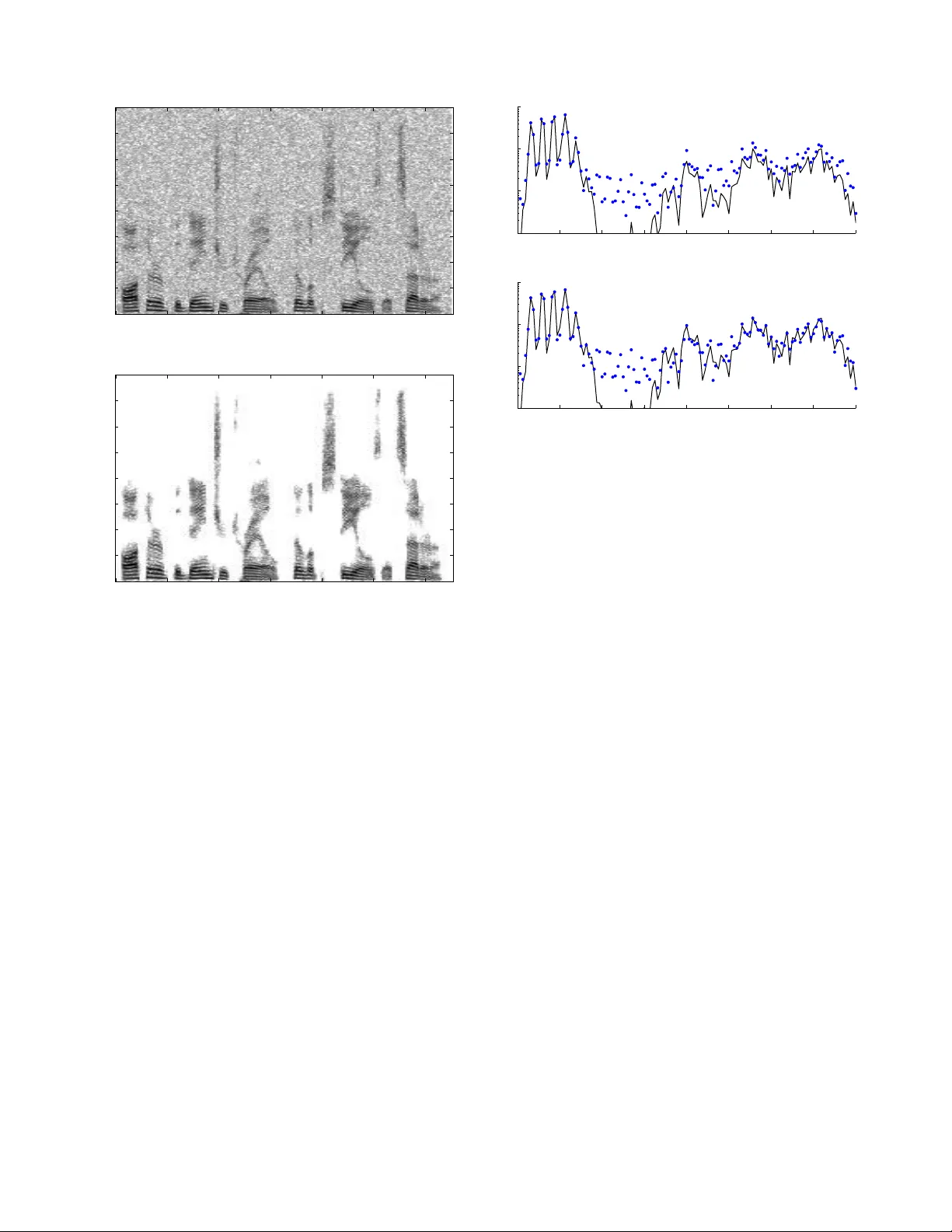
Leave a Comment