Bayesian Nonparametric Dictionary Learning for Compressed Sensing MRI
We develop a Bayesian nonparametric model for reconstructing magnetic resonance images (MRI) from highly undersampled k-space data. We perform dictionary learning as part of the image reconstruction process. To this end, we use the beta process as a …
Authors: Yue Huang, John Paisley, Qin Lin
1 Bayesian Nonparametric Dictionary Learning for Compressed Sensing MRI Y ue Huang † , John Paisle y † , Qin Lin, Xinghao Ding ‡ , Xueyang Fu and Xiao-ping Zhang, Senior Member , IEEE Abstract —W e develop a Bayesian nonparametric model for reconstructing magnetic r esonance images (MRI) from highly undersampled k -space data. W e perform dictionary learning as part of the image reconstruction pr ocess. T o this end, we use the beta process as a nonparametric dictionary learning prior for r epresenting an image patch as a sparse combination of dictionary elements. The size of the dictionary and the patch- specific sparsity pattern are inferred from the data, in addition to other dictionary learning variables. Dictionary learning is performed directly on the compressed image, and so is tailored to the MRI being considered. In addition, we in vestigate a total variation penalty term in combination with the dictionary learn- ing model, and show how the denoising property of dictionary learning removes dependence on regularization parameters in the noisy setting. W e derive a stochastic optimization algorithm based on Markov Chain Monte Carlo (MCMC) f or the Bayesian model, and use the alter nating direction method of multipliers (ADMM) for efficiently performing total variation minimization. W e present empirical results on sev eral MRI, which show that the proposed regularization framework can improve reconstruction accuracy over other methods. Index T erms —compressed sensing, magnetic resonance imag- ing, Bayesian nonparametrics, dictionary learning I . I N T R O D U C T I O N Magnetic resonance imaging (MRI) is a widely used tech- nique for visualizing the structure and functioning of the body . A limitation of MRI is its slow scan speed during data acquisition. Therefore, methods for accelerating the MRI process have been heavily researched. Recent advances in signal reconstruction from measurements sampled below the Nyquist rate, called compressed sensing (CS) [1], [2], ha ve had a major impact on MRI [3]. CS-MRI allows for significant undersampling in the Fourier measurement domain of MR images (called k -space), while still outputting a high-quality image reconstruction. While image reconstruction using this undersampled data is a case of an ill-posed inv erse problem, compressed sensing theory has sho wn that it is possible to reconstruct a signal from significantly fe wer measurements than mandated by traditional Nyquist sampling if the signal is sparse in a particular transform domain. This work supported by the National Natural Science Foundation of China (Nos. 30900328, 61172179, 61103121, 81301278), the Fundamental Research Funds for the Central Universities (Nos. 2011121051, 2013121023) and the Natural Science Foundation of Fujian Province of China (No. 2012J05160). Y . Huang, Q. Lin, X. Ding and X. Fu are with the Department of Communications Engineering at Xiamen University in Xiamen, Fujian, China. J. Paisley is with the Department of Electrical Engineering at Columbia Univ ersity in New Y ork, NY , USA. X.-P . Zhang is with the Department of Electrical and Computer Engineering at Ryerson University in T oronto, Canada. † Equal contributions. ‡ Corresponding author: dxh@xmu.edu.cn Motiv ated by the need to find a sparse domain for repre- senting the MR signal, a large body of literature now exists on reconstructing MRI from significantly undersampled k - space data. Existing improvements in CS-MRI mostly focus on ( i ) seeking sparse domains for the image, such as con- tourlets [4], [5]; ( ii ) using approximations of the ` 0 norm for better reconstruction performance with fewer measurements, for example ` 1 , FOCUSS, ` p quasi-norms with 0 < p < 1 , or using smooth functions to approximate the ` 0 norm [6], [7]; and ( iii ) accelerating image reconstruction through more efficient optimization techniques [8], [10], [29]. In this paper we present a modeling framework that is similarly motiv ated. CS-MRI reconstruction algorithms tend to fall into two categories: Those which enforce sparsity directly within some image transform domain [3]–[8], [10], [11], [12], and those which enforce sparsity in some underlying latent representa- tion of the image, such as an adaptive dictionary-based rep- resentation [9], [14]. Most CS-MRI reconstruction algorithms belong to the first category . For example Sparse MRI [3], the leading study in CS-MRI, performs MR image reconstruction by enforcing sparsity in both the wav elet domain and the total variation (TV) of the reconstructed image. Algorithms with image-lev el sparsity constraints such as Sparse MRI typically employ an of f-the-shelf basis, which can usually capture only one feature of the image. For example, wavelets recov er point- like features, while contourlets recover curve-like features. Since MR images contain a v ariety of underlying features, such as edges and textures, using a basis not adapted to the image can be considered a drawback of these algorithms. Finding a sparse basis that is suited to the image at hand can benefit MR image reconstruction, since CS theory shows that the required number of measurements is linked to the sparsity of the signal in the selected transform domain. Using a standard basis not adapted to the image under consideration will likely not provide a representation that can compete in sparsity with an adapted basis. T o this end, dictionary learning, which falls in the second group of algorithms, learns a sparse basis on image subregions called patches that is adapted to the image class of interest. Recent studies in the image processing literature hav e shown that dictionary learning is an effecti ve means for finding a sparse, patch-lev el represen- tation of an image [19], [20], [25]. These algorithms learn a patch-lev el dictionary by exploiting structural similarities between patches extracted from images within a class of inter- est. Among these approaches, adaptiv e dictionary learning— where the dictionary is learned directly from the image being considered—based on patch-level sparsity constraints usually outperforms analytical dictionary approaches in denoising, 2 super-resolution reconstruction, interpolation, inpainting, clas- sification and other applications, since the adaptiv ely learned dictionary suits the signal of interest [19]–[22]. Dictionary learning has previously been applied to CS- MRI to learn a sparse basis for reconstruction, e.g., [14]. W ith these methods, parameters such as the dictionary size and patch sparsity are preset, and algorithms are considered that are non-Bayesian. In this paper , we consider a ne w dictionary learning algorithm for CS-MRI that is motiv ated by Bayesian nonparametric statistics. Specifically , we consider a nonparametric dictionary learning model called BPF A [23] that uses the beta process to learn the sparse representation necessary for CS-MRI reconstruction. The beta process is an effectiv e prior for nonparametric learning of latent factor models; in this case the latent factors correspond to dictionary elements. While the dictionary size is therefore infinite in principle, through posterior inference the beta process learns a suitably compact dictionary in which the signal can be sparsely represented. W e organize the paper as follows. In Section II we revie w CS-MRI inv ersion methods and the beta process for dictionary learning. In Section III, we describe the proposed regulariza- tion frame work and algorithm. W e derive a Markov Chain Monte Carlo (MCMC) sampling algorithm for stochastic opti- mization of the dictionary variables in the objectiv e function. In addition, we consider including a sparse total variation (TV) penalty , for which we perform efficient optimization using the alternating direction method of multipliers (ADMM). W e then show the advantages of the proposed Bayesian nonparametric regularization framew ork on sev eral CS-MRI problems in Section IV. I I . B A C K G RO U N D A N D R E L A T E D W O R K W e use the following notation: Let x ∈ C N be a √ N × √ N MR image in vectorized form. Let F u ∈ C u × N , u N , be the undersampled Fourier encoding matrix and y = F u x ∈ C u represent the sub-sampled set of k -space measurements. The goal is to estimate x from the small fraction of k -space measurements y . For dictionary learning, let R i be the i th patch extraction matrix. That is, R i is a P × N matrix of all zeros except for a one in each row that extracts a vectorized √ P × √ P patch from the image, R i x ∈ C P for i = 1 , . . . , N . W e use o verlapping image patches with a shift of one pix el and allow a patch to wrap around the image at the boundaries for mathematical conv enience [15], [22]. All norms are extended to complex vectors when necessary , k a k p = ( P i | a i | p ) 1 /p , where | a i | is the modulus of the complex number a i . A. T wo approac hes to CS-MRI inver sion W e focus on single-channel CS-MRI inv ersion via optimiz- ing an unconstrained function of the form arg min x h ( x ) + λ 2 kF u x − y k 2 2 , (1) where kF u x − y k 2 2 is a data fidelity term, λ > 0 is a parameter and h ( x ) is a regularization function that controls properties of the image we want to reconstruct. As discussed in the introduction, the function h can take sev eral forms, but tends to fall into one of two categories according to whether image- lev el or patch-lev el information is considered. W e next revie w these two approaches. 1) Image-le vel sparse re gularization: CS-MRI with an image-lev el, or global regularization function h g ( x ) is one in which sparsity is enforced within a transform domain defined on the entire image. For example, in Sparse MRI [3] the regularization function is h g ( x ) = k W x k 1 + µ T V ( x ) , (2) where W is the wav elet basis and T V ( x ) is the total variation (spatial finite differences) of the image. Regularizing with this function requires that the image be sparse in the wav elet domain, as measured by the ` 1 norm of the wa velet coefficients k W x k 1 , which acts as a surrogate for ` 0 [1], [2]. The total variation term enforces homogeneity within the image by encouraging neighboring pixels to have similar values while allowing for sudden high frequency jumps at edges. The parameter µ > 0 controls the trade-off between the two terms. A variety of other image-level regularization approaches have been proposed along these lines, e.g., [4], [5], [7]. 2) P atch-le vel sparse r e gularization: An alternativ e to the image-lev el sparsity constraint h g ( x ) is a patch-le vel, or local regularization function h l ( x ) , which enforces that patches (square sub-regions of the image) have a sparse representation according to a dictionary . One possible general form of such a regularization function is, h l ( x ) = N X i =1 γ 2 k R i x − D α i k 2 2 + f ( α i , D ) , (3) where the dictionary matrix is D ∈ C P × K and α i is a K - dimensional vector in R K . An important difference between h l ( x ) and h g ( x ) is the additional function f ( α i , D ) . While image-lev el sparsity constraints fall within a predefined trans- form domain, such as the wav elet basis, the sparse dictionary domain can be unknown for patch-lev el regularization and learned from data. The function f enforces sparsity by learning a D for which α i is sparse. 1 For example, [9] uses K-SVD to learn D of f-line, and then approximately optimize the objectiv e function arg min α 1: N N X i =1 k R i x − D α i k 2 2 subject to k α i k 0 ≤ T , ∀ i, (4) using orthogonal matching pursuits (OMP) [21]. In this case, the L 0 penalty on the additional parameters α i make this a non-con ve x problem. Using this definition of h l ( x ) in (1), a local optimal solution can be found by an alternating minimization procedure [32]: First solve the least squares solution for x using the current values of α i and D , and then update α i and D , or only α i if D is learned off-line. B. Dictionary learning with beta pr ocess factor analysis T ypical dictionary learning approaches require a predefined dictionary size and, for each patch, the setting of either a 1 The dependence of h l ( x ) on α and D is implied in our notation. 3 Algorithm 1 Dictionary learning with BPF A 1) Construct a dictionary D = [ d 1 , . . . , d K ] , with d k ∼ N (0 , P − 1 I P ) , k = 1 , . . . , K. 2) Dra w a probability π k ∈ [0 , 1] for each d k : π k ∼ B eta ( cγ /K, c (1 − γ /K )) , k = 1 , . . . , K . 3) Dra w precision values for noise and each weight γ ε ∼ Gam ( g 0 , h 0 ) , γ s ∼ Gam ( e 0 , f 0 ) . 4) F or the i th patch in x : a) Dra w the vector s i ∼ N (0 , γ − 1 s I K ) . b) Dra w the binary vector z i with z ik ∼ B er n ( π k ) . c) Define α i = s i ◦ z i by an element-wise product. d) Sample noisy patch R i x ∼ N ( D α i , γ − 1 ε I P ) . 5) Construct the image x as the average of all R i x that ov erlap on a giv en pixel. sparsity le vel T , or an error threshold to determine ho w man y dictionary elements are used. In both cases, if the settings do not agree with ground truth, the performance can signifi- cantly degrade. Instead, we consider a Bayesian nonparametric method called beta process factor analysis (BPF A) [23], which has been shown to successfully infer both of these values, as well as have competitive performance with algorithms in sev eral application areas [23]–[26], and see [33]–[36] for related algorithms. The beta process is driv en by an under- lying Poisson process, and so it’ s properties as a Bayesian nonparametric prior are well understood [27]. Originally used for surviv al analysis in the statistics literature, its use for latent factor modeling has been significantly increasing within the machine learning community [23]–[26], [28], [33]–[36]. 1) Generative model: W e giv e the original hierarchical prior structure of the BPF A model in Algorithm 1, extending this to complex-v alued dictionaries in Section III-A. W ith this approach, the model constructs a dictionary matrix D ∈ R P × K ( C P × K below) of i.i.d. random variables, and assigns probability π k to vector d k . The parameters for these probabil- ities are set such that most of the π k are expected to be small, with a few large. In Algorithm 1 we use an approximation to the beta process. 2 Under this parameterization, each patch R i x extracted from the image x is modeled as a sparse weighted combination of the dictionary elements, as determined by the element-wise product of z i ∈ { 0 , 1 } K with the Gaussian vector s i . What makes the model nonparametric is that for many values of k , the values of z ik will equal zero for all i since π k will be very small; the model learns the number of these unused dictionary elements and their inde x v alues from the data. Therefore, the v alue of K should be set to a lar ge number that is more than the e xpected size of the dictionary . It can be shown that, under the assumptions of this prior , in the limit K → ∞ , the number of dictionary elements used by a patch is Poisson ( γ ) distrib uted and the total number of dictionary elements used by the data grows like cγ ln N , where N is the number of patches [28]. The parameters of 2 For a finite c > 0 and γ > 0 , the random measure H = P K k =1 π k δ d k con ver ges weakly to a beta process as K → ∞ [27], [24]. T ABLE I P E AK S I GN A L - TO - N O I S E R ATI O ( P S N R ) F O R I M AG E D E NO I S E D B Y B P FA . C O MPA R ED W I TH K - S V D U S IN G C O RR E C T ( M A TC H ) A N D I N C O RR E C T ( M IS M A T C H ) N O IS E PA R A ME T E R . σ K-SVD denoising (PSNR) BPF A denoising (PSNR) Match Mismatch Results Learned noise 20/255 32.28 28.94 32.88 20.43/255 25/255 31.08 28.60 31.81 25.46/255 30/255 29.99 28.35 30.94 30.47/255 (a) Noisy image (b) Denoising by BPF A 0 20 40 60 80 100 0.1 0.2 0.3 0.4 0.5 (c) Dictionary probabilities 0 1 2 3 4 5 6 7 8 9 0 0.05 0.1 0.15 0.2 0.25 0.3 (d) Dictionary elements per patch Fig. 1. (a)-(b) An example of denoising by BPF A (image scaled to [0,1]). (c) Shows the final probabilities of the dictionary elements and (d) shows a distribution on the number of dictionary elements used per patch. the model include c, γ , e 0 , f 0 , g 0 , h 0 and K ; we discuss setting these values in Section IV. 2) Relationship to K-SVD: Another widely used dictionary learning method is K-SVD [20]. Though they are models for the same problem, BPF A and K-SVD hav e some significant differences that we briefly discuss. K-SVD learns the sparsity pattern of the coding vector α i using the OMP algorithm [21] for each i . Holding the sparsity pattern fixed, it then updates each dictionary element and dimension of α jointly by a rank one approximation to the residual. Unlike BPF A, it learns as many dictionary elements as are given to it, so K should be set wisely . BPF A on the other hand automatically prunes unneeded elements, and updates the sparsity pattern by using the posterior distribution of a Bernoulli process, which is significantly different from OMP . It updates the weights and the dictionary from their Gaussian posteriors as well. Because of this probabilistic structure, we deriv e a sampling algorithm for these variables that takes adv antage of marginalization, and naturally learns the auxiliary variables γ ε and γ s . 3) Example denoising problem: As we will see, the rela- tionship of dictionary learning to CS-MRI is essentially as a denoising step. T o this end, we briefly illustrate BPF A on a denoising problem. Denoising of an image using dictionary 4 learning proceeds by first learning the dictionary representa- tion of each patch, R i x ≈ D α i . The denoised reconstruction of x using BPF A is then x BPF A = 1 P P i R T i D α i . W e show an example using 6 × 6 patches extracted from the noisy 512 × 512 image shown in Figure 1(a). In Figure 1(b) we show the resulting denoised image. For this problem we truncated the dictionary size to K = 108 and set all other model parameters to one. In Figures 1(c) and 1(d) we show some statistics from dictionary learning. For example, Figure 1(c) shows the values of π k sorted, where we see that fewer than 100 elements are used by the data, many of which are very sparsely used. Figure 1(d) shows the empirical distribution of the number of elements used per patch. W e see the ability of the model to adapt the sparsity to the complexity of the patch. In T able I we show PSNR results for three noise variance lev els. For K-SVD, we consider the case when the error parameter matches the ground truth, and when it mismatches it by a magnitude of five. As expected, when K-SVD does not hav e an appropriate parameter setting the performance suffers. BPF A on the other hand adaptively infers this value, which helps improve the denoising. I I I . C S - M R I W I T H B P FA A N D T V P E N A L T Y W e next present our approach for reconstructing single- channel MR images from highly undersampled k -space data. In reference to the discussion in Section II, we consider a sparsity constraint of the form arg min x,ϕ λ g h g ( x ) + h l ( x ) + λ 2 kF u x − y k 2 2 , (5) h g ( x ) := T V ( x ) , h l ( x ) := N X i =1 γ ε 2 k R i x − D α i k 2 2 + f ( ϕ i ) . For the local regularization function h l ( x ) we use BPF A as gi ven in Algorithm 1 in Section II-B. The parameters to be optimized for this penalty are contained in the set ϕ i = { D , s i , z i , γ ε , γ s , π } , and are defined in Algorithm 1. W e note that only s i and z i vary in i , while the rest are shared by all patches. The regularization term γ ε is a model variable that corresponds to an in v erse variance parameter of the multiv ariate Gaussian likelihood. This likelihood is equiv alently viewed as the squared error penalty term in h l ( x ) in (5). This term acts as the sparse basis for the image and also aids in producing a denoised reconstruction, as discussed in Sections II-B, III-B and IV -B. For the global regularization function h g ( x ) we use the total variation of the image. This term encourages homogeneity within contiguous regions of the image, while still allowing for sharp jumps in pixel value at edges due to the underlying ` 1 penalty . The regularization parameters λ g , γ ε and λ control the trade-off between the terms in this optimization. Since we sample a new value of γ ε with each iteration of the algorithm discussed shortly , this trade-off is adaptiv ely changing. For the total variation penalty T V ( x ) we use the isotropic TV model. Let ψ i be the 2 × N difference operator for pixel i . Each row of ψ i contains a 1 centered on pixel i , and the first row also has a − 1 on the pixel directly above pixel i , while the second has a − 1 corresponding to the pixel to the right, and zeros elsewhere. Let Ψ = [ ψ T 1 , . . . , ψ T N ] T be the resulting 2 N × N dif ference matrix for the entire image. The TV coefficients are β = Ψ x ∈ C 2 N , and the isotropic TV penalty is T V ( x ) = P i k ψ i x k 2 = P i q | β | 2 2 i − 1 + | β | 2 2 i , where i ranges over the pixels in the MR image. For optimization we use the alternating direction method of multipliers (ADMM) [31], [30]. ADMM works by performing dual ascent on the augmented Lagrangian objectiv e function introduced for the total variation coefficients. For completeness, we giv e a brief revie w of ADMM in the appendix. A. Algorithm W e present an algorithm for finding a local optimal solution to the non-con v ex objecti ve function giv en in (5). W e can write this objective as L ( x , ϕ ) = λ g P i k ψ i x k 2 + P i γ ε 2 k R i x − D α i k 2 2 + P i f ( ϕ i ) + λ 2 kF u x − y k 2 2 . (6) W e seek to minimize this function with respect to x and the dictionary learning variables ϕ i = { D , s i , z i , γ ε , γ s , π } . Our first step is to put the objectiv e into a more suitable form. W e begin by defining the TV coefficients for the i th pixel as β i := [ β 2 i − 1 β 2 i ] T = ψ i x . W e introduce the vector of Lagrange multipliers η i , and then split β i from ψ i x by relaxing the equality via an augmented Lagrangian. This results in the objectiv e function L ( x , β , η , ϕ ) = N X i =1 λ g k β i k 2 + η T i ( ψ i x − β i ) + ρ 2 k ψ i x − β i k 2 2 + N X i =1 γ ε 2 k R i x − D α i k 2 2 + f ( ϕ i ) + λ 2 kF u x − y k 2 2 . (7) From the ADMM theory [32], this objective will have (local) optimal values β ∗ i and x ∗ with β ∗ i = ψ i x ∗ , and so the equality constraints will be satisfied [31]. 3 Optimizing this function can be split into three separate sub-problems: one for TV , one for BPF A and one for updating the reconstruction x . Follo wing the discussion of ADMM in the appendix, we define u i = (1 /ρ ) η i and complete the square in the first line of (7). W e then cycle through the following three sub-problems, ( P 1) β 0 i = arg min β λ g k β k 2 + ρ 2 k ψ i x − β + u i k 2 2 , u 0 i = u i + ψ i x − β 0 i , i = 1 , . . . , N , ( P 2) ϕ 0 = arg min ϕ P i γ ε 2 k R i x − D α i k 2 2 + f ( ϕ i ) , ( P 3) x 0 = arg min x P i ρ 2 k ψ i x − β 0 i + u 0 i k 2 2 + P i γ 0 ε 2 k R i x − D 0 α 0 i k 2 2 + λ 2 kF u x − y k 2 2 . Solutions for sub-problems P 1 and P 3 are globally optimal (conditioned on the most recent values of all other parameters). W e cannot solve P 2 analytically since the optimal v alues for the set of all BPF A v ariables do not 3 For a fixed D , α 1: N and x the solution is also globally optimal. 5 Algorithm 2 Outline of algorithm Input: y – Undersampled k -space data Output: x – Reconstructed MR image Initialize: x = F H u y and each u i = 0 . Sample D from prior . Step 1. P 1 : Optimize each β i via shrinkage. Step 2. Update Lagrange multiplier vectors u i . Step 3. P 2 : Gibbs sample BPF A variables once. Step 4. P 3 : Solve for x using Fourier domain. if not con ver ged then return to Step 1. hav e a closed form solution. Our approach for P 2 is to use stochastic optimization by Gibbs sampling each v ariable of BPF A conditioned on current v alues of all other variables. W e next present the updates for each sub-problem. W e giv e an outline in Algorithm 2. 1) Algorithm for P1 (total variation): W e can solve for β i exactly for each pixel i = 1 , . . . , N by using a generalized shrinkage operation [31], β 0 i = max k ψ i x + u i k 2 − λ g ρ , 0 · ψ i x + u i k ψ i x + u i k 2 . (8) W e recall that β i corresponds to the 2-dimensional TV coefficients for pixel i , with differences in one direction vertically and horizontally . W e then update the corresponding Lagrange multiplier, u 0 i = u i + ψ i x − β 0 i . 2) Algorithm for P2 (BPF A): W e update the parameters of BPF A using Gibbs sampling. W e are therefore stochastically optimizing (7), but only for this sub-problem. W ith reference to Algorithm 1, the P2 sub-problem entails sampling new values for the complex dictionary D , the binary vectors z i and real-valued weights s i (with which we construct α i = s i ◦ z i through the element-wise product), the precisions γ ε and γ s , and the probabilities π 1: K , with π k giving the probability that z ik = 1 . In principle, there is no limit to the number of samples that can be made, with the final sample giving the updates used in the other sub-problems. W e found that a single sample is sufficient in practice and leads to a faster algorithm. W e describe the sampling procedure below . a) Sample dictionary D : W e define the P × N matrix X = [ R 1 x , . . . , R N x ] , which is a complex matrix of all vectorized patches extracted from the image x . W e also define the K × N matrix α = [ α 1 , . . . , α N ] containing the dictionary weight coefficients for the corresponding columns in X such that D α is an approximation of X to which we add noise from a circularly-symmetric complex normal distribution. The update for the dictionary D is D = X α T ( αα T + ( P /γ ε ) I P ) − 1 + E , (9) E p, : ind ∼ C N (0 , ( γ ε αα T + P I P ) − 1 ) , p = 1 , . . . , P , where E p, : is the p th row of E . T o sample this, we can first draw E p, : from a multiv ariate Gaussian distribution with this cov ariance structure, followed by an i.i.d. uniform rotation of each value in the complex plane. W e note that the first term in Equation (9) is the ` 2 -regularized least squares solution for D . The addition of correlated Gaussian noise in the complex plane generates the sample from the conditional posterior of D . Since both the number of pixels and γ ε will tend to be very large, the variance of the noise is small and the mean term dominates the update for D . b) Sample sparse coding α i : Sampling α i entails sam- pling s ik and z ik for each k . W e sample these v alues us- ing block sampling. W e recall that to block sample two variables from their joint conditional posterior distribution, ( s, z ) ∼ p ( s, z |− ) , one can first sample z from the marginal distribution, z ∼ p ( z |− ) , and then sample s | z ∼ p ( s | z , − ) from the conditional distribution. The other sampling direction is possible as well, but for our problem sampling z → s | z is more efficient for finding a mode of the objectiv e function. W e define r i, − k to be the residual error in approximating the i th patch with the current values from BPF A minus the k th dictionary element, r i, − k = R i x − P j 6 = k ( s ij z ij ) d j . W e then sample z ik from its conditional posterior Bernoulli distribution z ik ∼ p ik δ 1 + q ik δ 0 , where following a simplification, p ik ∝ π k 1 + ( γ ε /γ s ) d H k d k − 1 2 × (10) exp n γ ε 2 Re( d H k r i, − k ) 2 / ( γ s /γ ε + d H k d k ) o , q ik ∝ 1 − π k . (11) The symbol H denotes the conjugate transpose. The proba- bilities can be obtained by dividing both of these terms by their sum. W e observe that the probability that z ik = 1 takes into account how well dictionary element d k correlates with the residual r i, − k . After sampling z ik we sample the corre- sponding weight s ik from its conditional posterior Gaussian distribution, s ik | z ik ∼ N z ik Re( d H k r i, − k ) γ s /γ ε + d H k d k , 1 γ s + γ ε z ik d H k d k ! . (12) When z ik = 1 , the mean of s ik is the regularized least squares solution and the variance will be small if γ ε is large. When z ik = 0 , s ik can is sampled from the prior , but does not factor in the model in this case. c) Sample γ ε and γ s : W e next sample from the condi- tional gamma posterior distribution of the noise precision and weight precision, γ ε ∼ Gam g 0 + 1 2 P N , h 0 + 1 2 P i k R i x − D α i k 2 2 , (13) γ s ∼ Gam ( e 0 + 1 2 P i,k z ik , f 0 + 1 2 P i,k z ik s 2 ik ) . (14) The expected value of each variable is the first term of the distribution di vided by the second, which is close to the in verse of the av erage empirical error for γ ε . d) Sample π k : Sample each π k from its conditional beta posterior distribution, π k ∼ B eta a 0 + P N i =1 z ik , b 0 + P N i =1 (1 − z ik ) . (15) The parameters to the beta distribution include counts of how many times dictionary element d k was used by a patch. 6 3) Algorithm for P3 (MRI r econstruction): The final sub- problem is to reconstruct the image x . Our approach takes advantage of the Fourier domain similar to other methods, e.g. [14], [30]. The corresponding objectiv e function is x 0 = arg min x N X i =1 ρ 2 k ψ i x − β i + u i k 2 2 + N X i =1 γ ε 2 k R i x − D α i k 2 2 + λ 2 kF u x − y k 2 2 . Since this is a least squares problem, x has a closed form solution that satisfies ρ Ψ T Ψ + γ ε P i R T i R i + λ F H u F u x = (16) ρ Ψ T ( β − u ) + γ ε P x BPF A + λ F H u y . W e recall that Ψ is the matrix of stacked ψ i . The vector β is also obtained by stacking each β i and u is the vector formed by stacking u i . The vector x BPF A is the denoised reconstruction from BPF A using the current D and α 1: N , which results from the definition x BPF A = 1 P P i R T i D α i . W e observe that in verting the left N × N matrix is compu- tationally prohibitiv e since N is the number of pixels in the image. Fortunately , given the form of the matrix in Equation (16) we can use the procedure described in [14] and simplify the problem by working in the Fourier domain. This allows for element-wise updates in k -space, followed by an in verse Fourier transform. W e represent x as x = F H θ , where θ is the Fourier transform of x . W e then take the Fourier transform of each side of Equation (16) to give F ρ Ψ T Ψ + γ ε P i R T i R i + λ F H u F u F H θ = (17) ρ F Ψ T ( β − u ) + γ ε F P x BPF A + λ F F H u y . The left-hand matrix simplifies to a diagonal matrix, F ρ Ψ T Ψ + γ ε P i R T i R i + λ F H u F u F H = (18) ρ Λ + γ ε P I N + λI u N . T erm-by-term this results as follows: The product of the finite difference operator matrix Ψ with itself yields a circulant matrix, which has the rows of the Fourier matrix F as its eigen vectors and eigenv alues equal to Λ = F Ψ T Ψ F H . The matrix R T i R i is a matrix of all zeros, except for ones on the diagonal entries that correspond to the indices of x associated with the i th patch. Since each pixel appears in P patches, the sum over i giv es P I N , and the Fourier product cancels. The final diagonal matrix I u N also contains all zeros, except for ones along the diagonal corresponding to the indices in k -space that are measured, which results from F F H u F u F H . Since the left matrix is diagonal we can perform element- wise updating of the Fourier coefficients θ , θ i = ρ F i Ψ T ( β − u ) + γ ε P F i x BPF A + λ F i F H u y ρ Λ ii + γ ε P + λ F i F H u 1 . (19) W e observe that the rightmost term in the numerator and denominator equals zero if i is not a measured k -space location. W e in vert θ via the inv erse Fourier transform F H to obtain the reconstructed MR image x 0 . (a) Random 25% (b) Cartesian 30% (c) Radial 25% Fig. 2. The three masks considered for a giv en sampling percentage. B. Discussion on λ In noise-free compressed sensing, the fidelity term λ can tend to infinity giving an equality constraint for the measured k -space values [1]. Howev er , when y is noisy the setting of λ is critical for most CS-MRI algorithms since this parameter controls the level of denoising in the reconstructed image. W e note that a feature of dictionary learning CS-MRI approaches is that λ can still be set to a very lar ge value, and so parameter selection isn’t necessary here. This is because a denoised version of the image is obtained through dictionary learning ( x BPF A in this paper) and can be taken as the denoised reconstruction. In Equation (19), we observe that by setting λ to a large v alue, we are ef fectiv ely fixing the measured k -space values and using the k -space projection of BPF A and TV to fill in the missing values. The reconstruction x will be noisy , but hav e artifacts due to sub-sampling removed. The output image x BPF A is a denoised version of x using BPF A in essentially the same manner as in Section II-B3. Therefore, the quality of our algorithm depends largely on the quality of BPF A as an image denoising algorithm [25]. W e show examples of this using synthetic and clinical data in Sections IV -B and IV -E. I V . E X P E R I M E N TA L R E S U LT S W e e v aluate the proposed algorithm on real-valued and complex-v alued MRI, and on a synthetic phantom. W e con- sider three sampling masks: 2D random sampling, Carte- sian sampling with random phase encodes (1D random), and pseudo radial sampling. 4 W e show an example of each mask in Figure 2. W e consider a variety of sampling rates for each mask. As a performance measure we use PSNR, and also consider SSIM [37]. W e compare with three other algorithms: Sparse MRI [3] 5 , which as discussed above is a combination of wa velets and total variation, DLMRI [14] 6 , which is a dictionary learning method based on K-SVD, and PBD W [15] 7 , which is patch-based method that uses directional wav elets and therefore places greater restrictions on the dictionary . W e use the publicly av ailable code for these algorithms indicated abov e and used the built-in parameter settings, or those indicated in the relev ant papers. W e also compare with the BPF A algorithm without using total v ariation by setting λ g = 0 . 4 W e used codes referenced in [3], [8], [10] to generate these masks. 5 http://www .eecs.berk eley .edu/ ∼ mlustig/Software.html 6 http://www .ifp.illinois.edu/ ∼ yoram/DLMRI- Lab/Documentation.html 7 http://www .quxiaobo.or g/index publications.html 7 (a) Zero filling (b) BPF A reconstruction ( x ) (c) BPF A denoising ( x BPF A ) (d) T otal variation reconstruction (e) Dictionary (magnitude) 0 20 40 60 80 0.02 0.04 0.06 0.08 0.1 0.12 0.14 0.16 0.18 0.2 0.22 (f) Dictionary probabilities 0 1 2 3 4 5 6 7 8 9 0 0.1 0.2 0.3 0.4 0.5 0.6 (g) Dictionary elements per patch Fig. 3. GE data with noise ( σ = 0 . 1 ) and 30% Cartesian sampling. BPF A (b) reconstructs the original noisy image, and (c) denoises the reconstruction simultaneously . (d) TV denoises as part of the reconstruction. Also shown are the dictionary learning variables sorted by π k . (e) the dictionary , (f) the distribution on the dictionary , π k . (g) The normalized histogram of number of the dictionary elements used per patch. A. Set-up For all images, we extract 6 × 6 patches where each pixel defines the upper left corner of a patch and wrap around the image at the boundaries; we in vestigate different patch sizes later to show that this is a reasonable size. W e initialize x by zero-filling in k -space. W e use a dictionary with K = 108 initial dictionary elements, recalling that the final number of dictionary elements will be smaller due to the sparse BPF A prior . If 108 is found to be too small, K can be increased with the result being a slower inference algorithm. 8 W e ran 1000 iterations and use the results of the last iteration. For regularization parameters, we set the data fidelity term λ = 10 100 . W e are therefore effecti vely requiring equality with the measured values of k -space and allowing BPF A to fill in the missing values, as well as giv e a denoised reconstruction, as discussed in Section III-B and highlighted below in Sections IV -B and IV -E. After trying se veral values, we also found λ g = 10 and ρ = 1000 to give good results. W e set the BPF A hyperparameters as c = γ = e 0 = f 0 = g 0 = h 0 = 1 . These settings result in a relativ ely non-informative prior given the amount of data we hav e. Howe ver , we note that our algorithm was robust to these values, since the data ov erwhelms these prior values when calculating posterior distributions. B. Experiments on a GE phantom W e consider a noisy synthetic e xample to highlight the advantage of dictionary learning for CS-MRI. In Figure 3 we show results on a 256 × 256 GE phantom with additiv e noise having standard deviation σ = 0 . 1 . In this experiment we use BPF A without TV to reconstruct the original image using 30% Cartesian sampling. W e show the reconstruction using zero-filling in Figure 3(a). Since λ = 10 100 , we see in Figure 3(b) that BPF A essentially helps reconstruct the underlying noisy image for x . Howe ver , using the denoising property of the BPF A model shown in Figure 1, we obtain the denoised reconstruction of Figure 3(c) by focusing on x BPF A from Equation (16). This is in contrast with the best result we could obtain with TV in Figure 3(d), which places the TV penalty on the reconstructed image. As discussed, for TV the setting of λ relati ve to λ g is important. W e set λ = 1 and swept through λ g ∈ (0 , 0 . 15) , showing the result with highest PSNR in Figure 3(d). Similar to Figure 1 we show statistics from the BPF A model in Figures 3(e)-(g). W e see that roughly 80 dictionary elements were used (the unused noisy elements in Figure 3(e) are draws from the prior). W e note that 2 . 28 elements were used on av erage by a patch given that at least one was used, which discounts the black regions. C. Experiments on r eal-valued (synthetic) MRI For our synthetic MRI experiments, we consider two pub- licly av ailable real-valued 512 × 512 MRI 9 of a shoulder and lumbar . W e construct these problems by applying the relev ant sampling mask to the projection of real-valued MRI into k - space. Though using such real-v alued MRI data may not reflect clinical reality , we include this idealized setting to provide a complete set of experiments similar to other papers [3], [14], [15]. W e ev aluate the performance of our algorithm using PSNR and compare with Sparse MRI [3], DLMRI [14] and PBD W [15]. Although the original data is real-valued, we learn complex dictionaries since the reconstructions are complex. W e consider our algorithm with and without the total variation penalty , denoted BPF A+TV and BPF A, respectiv ely . 8 As discussed in Section II-B, in theory K can be infinitely large. 9 www3.americanradiology .com/pls/web1/wwimggal.vmg/wwimgg al.vmg 8 T ABLE II P S NR R E SU L T S F O R R E AL - V AL U E D L U MB A R M R I A S F U NC T I O N O F S A MP LI N G P E R C EN T AG E A N D M A SK ( C A RT E SI AN W I T H R A N D OM P H AS E E N CO DE S , 2 D R AN DO M A N D P S E U D O R A DI A L ) . Mask Samp% BPF A+TV BPF A DLMRI SparseMRI PBD W Cart. 10 32.48 32.03 31.02 30.24 31.74 20 36.07 35.84 33.92 33.44 35.19 25 38.78 38.53 36.56 35.50 37.43 30 41.08 40.12 38.87 35.57 39.23 35 41.05 40.96 38.85 37.66 39.24 Rand. 10 42.82 40.81 38.25 25.87 37.09 20 44.35 41.80 40.11 27.80 37.86 25 48.11 47.09 43.51 37.22 43.65 30 49.36 48.55 44.93 38.72 45.50 35 50.20 49.19 45.87 41.70 46.85 Rad. 10 35.16 33.33 32.91 29.35 31.46 20 41.69 41.18 38.38 35.69 38.01 25 43.75 43.40 40.29 38.59 40.25 30 45.22 44.95 41.86 37.37 42.11 35 46.85 46.45 43.09 39.74 43.72 T ABLE III P S NR R E SU L T S F O R R E AL - V AL U E D S H OU L D E R M R I A S F U N C T I O N O F S A MP LI N G P E R C EN T AG E A N D M A SK ( C A RT E SI AN W I T H R A N D OM P H AS E E N CO D E S , 2 D R A N D O M A N D P S EU D O R A D I AL ) . Mask Samp% BPF A+TV BPF A DLMRI SparseMRI PBD W Cart. 10 32.65 30.79 31.02 27.65 28.88 20 36.96 35.77 34.52 30.64 32.10 25 38.45 37.97 35.69 32.44 34.12 30 41.43 41.22 38.11 34.26 36.73 35 41.33 41.14 38.44 34.50 36.76 Rand. 10 41.00 39.96 38.18 30.72 36.48 20 43.53 42.40 39.38 32.08 39.39 25 45.43 45.44 42.58 40.81 41.31 30 46.89 46.86 44.03 43.47 43.12 35 47.95 47.87 45.01 44.89 44.45 Rad. 10 34.30 33.88 33.27 29.18 31.60 20 39.41 39.47 38.06 35.50 36.38 25 41.40 41.52 39.73 38.70 38.21 30 43.14 43.45 41.20 39.98 40.30 35 44.69 44.99 42.58 39.11 41.72 W e present the PSNR results for all sampling masks and rates in T ables II and III. From these v alues we see the compet- itiv e performance of the propose dictionary learning algorithm. W e also see a slight improvement by the addition of the TV penalty . As expected, we observe that 2D random sampling produced the best results, followed by pseudo-radial sampling and Cartesian sampling, which is due to their decreasing lev el of incoherence, with greater incoherence producing artifacts that are more noise-like [3]. Since BPF A is good at denoising images, the algorithm naturally performs well in this setting. In Figures 4 and 5 we show the absolute value of the residuals of dif ferent algorithms using one experiment from each MRI. W e see an improvement using the proposed method, which has more noise-like errors. D. Experiments on complex-valued MRI W e also consider two clinically obtained complex-v alued MRI: W e use the T2-weighted brain MRI from [4], which is a 256 × 256 MRI of a healthy volunteer from a 3T Siemens (a) BPF A+TV (b) PBDW (c) DLMRI (d) Sparse MRI Fig. 4. Absolute errors for 30% Cartesian sampling of synthetic lumbar MRI. 0 0.05 0.1 0.15 (a) BPF A+TV 0 0.05 0.1 0.15 (b) PBDW 0 0.05 0.1 0.15 (c) DLMRI 0 0.05 0.1 0.15 (d) Sparse MRI Fig. 5. Absolute errors for 20% radial sampling of the shoulder MRI. T rio Tim MRI scanner using the T2-weighted turbo spin echo sequence (TR/TE = 6100/99 ms, 220 × 220 mm field of view , 3 mm slice thickness). W e also use an MRI scan of a lemon obtained from the Research Center of Magnetic Resonance and Medical Imaging at Xiamen Uni versity (TE = 32 ms, size = 256 × 256, spin echo sequence, TR/TE=10000/32 ms, FO V= 70 × 70 mm 2 , 2-mm slice thickness). This MRI is from a 7T/160mm bore V arian MRI system (Agilent T echnologies, Santa Clara, CA, USA) using a quadrature-coil probe. For the brain MRI e xperiment we use both PSNR and 9 T ABLE IV P S NR / S S IM R E SU L T S F O R C O MP L E X - V A L UE D B R A I N M R I A S A F U N CT I O N O F S A M P L I NG P E R C E N T AG E . S A M P L IN G M A S K S I N C L U D E C A RTE S I A N S A MP LI N G W I T H R A ND O M P H A S E E N C O D E S , 2 D R A ND O M S A M P LI N G A N D P S E U DO R A DI A L S A M P LI N G . Mask Sample % BPF A+TV BPF A DLMRI Sparse MRI PBDW Zero-filling Cartesian 25 35.62 / 0.951 34.86 / 0.948 29.90 / 0.812 25.29 / 0.696 34.69 / 0.935 24.13 / 0.591 30 38.64 / 0.968 37.70 / 0.965 31.54 / 0.849 26.16 / 0.745 37.24 / 0.957 24.55 / 0.614 35 39.36 / 0.972 38.87 / 0.971 32.35 / 0.863 27.35 / 0.795 37.90 / 0.963 24.94 / 0.616 40 41.09 / 0.977 40.45 / 0.976 33.60 / 0.876 29.82 / 0.845 39.23 / 0.969 26.28 / 0.667 Random 10 31.57 / 0.923 31.24 / 0.920 29.38 / 0.821 24.85 / 0.756 31.15 / 0.921 23.23 / 0.536 15 36.49 / 0.963 35.44 / 0.961 30.16 / 0.774 22.68 / 0.651 34.22 / 0.942 21.18 / 0.493 20 38.83 / 0.962 38.38 / 0.964 31.62 / 0.804 26.28 / 0.672 36.29 / 0.960 23.52 / 0.504 25 40.75 / 0.979 40.00 / 0.973 32.83 / 0.862 31.16 / 0.934 37.62 / 0.968 26.58 / 0.582 30 42.70 / 0.984 42.24 / 0.984 34.09 / 0.887 31.90 / 0.965 39.38 / 0.976 27.67 / 0.630 Radial 10 30.76 / 0.914 30.68 / 0.914 27.78 / 0.680 19.79 / 0.482 30.78 / 0.886 19.06 / 0.367 15 34.00 / 0.949 33.79 / 0.950 29.49 / 0.734 22.07 / 0.640 33.99 / 0.937 20.87 / 0.498 20 36.92 / 0.967 36.60 / 0.967 30.78 / 0.768 24.22 / 0.739 36.34 / 0.958 22.57 / 0.537 25 39.72 / 0.977 39.37 / 0.977 31.91 / 0.794 26.64 / 0.797 38.38 / 0.970 24.34 / 0.574 30 41.81 / 0.982 41.54 / 0.982 32.77 / 0.807 28.20 / 0.827 39.74 / 0.975 25.43 / 0.600 (a) Original (b) BPF A+TV (c) BPF A (d) PBDW (e) DLMRI 0 200 400 600 800 1000 28 30 32 34 36 38 40 BPFA+TV BPFA (f) PSNR vs iteration (g) BPF A+TV error (h) BPF A error (i) PBDW error (j) DLMRI error Fig. 6. Reconstruction results for 25% pseudo radial sampling of a complex-valued MRI of the brain. SSIM as performance measures. W e show these values in T able IV for each algorithm, sampling mask and sampling rate. As with the synthetic MRI, we see that our algorithm performs competitiv ely with the state-of-the-art. W e also see the significant improvement of all algorithms over zero-filling. Example reconstructions are shown for each MRI dataset in Figures 6 and 7. Also in Figure 7 are PSNR values for the lemon MRI. W e see from the absolute error residuals for these experiments that the BPF A algorithm learns a slightly finer detail structure compared with other algorithms, with the errors being more noise-like. W e also show the PSNR of BPF A+TV and BPF A as a function of iteration. As is evident, the algorithm does not necessarily need all 1000 iterations, but performs competitively even in half that number . 10 3 10 4 10 5 10 6 28 29 30 31 32 33 34 BPFA reconstru ction BPFA denoising Fig. 8. PSNR vs λ in the noisy setting ( σ = 0 . 03 ) for the complex-value brain MRI with 30% 2D random sampling. E. Experiments in the noisy setting The MRI we have considered thus far have been essentially noiseless. For some MRI machines this may be an unrealistic assumption. W e continue our ev aluation of noisy MRI begun with the toy GE phantom in Section IV -B by ev aluating how 10 (a) Original (b) BPF A+TV : PSNR = 39.64 (c) BPF A: PSNR = 38.21 (d) PBDW : PSNR = 37.89 (e) DLMRI: PSNR = 35.05 0 200 400 600 800 1000 30 31 32 33 34 35 36 37 38 39 40 BPF A+ T V BPFA (f) PSNR vs iteration (g) BPF A+TV error (h) BPF A error (i) PBDW error (j) DLMRI error Fig. 7. Reconstruction results for 35% 2D random sampling of a complex-valued MRI of a lemon. (a) Zero filling (b) BPF A reconstruction ( x ) (c) BPF A denoising ( x BPF A ) (d) DLMRI Fig. 9. The denoising properties of dictionary learning on noisy complex- valued MRI with 35% Cartesian sampling and σ = 0 . 03 . our model performs on clinically obtained MRI with additive noise. W e show BPF A results without TV to highlight the dictionary learning features, but note that results with TV provide a slight improv ement in terms of PSNR and SSIM. W e again consider the brain MRI and use additiv e complex white Gaussian noise ha ving standard de viation σ = 0 . 01 , 0 . 02 , 0 . 03 . For all experiments we use the original noise-free MRI as the ground truth. T ABLE V P S NR F O R 3 5 % C A RT E S IA N S A MP L I N G O F C O MP L E X - V A L UE D B R A I N M R I F O R V A R I O U S N O I S E S TA N D A R D D E VI A T I O NS . ( λ = 10 100 ) Reconstruction method σ = 0 σ = 0 . 01 σ = 0 . 02 σ = 0 . 03 BPF A–reconstruction 38.87 37.25 33.77 31.08 BPF A–denoising 37.99 37.19 34.43 32.39 DLMRI 32.35 32.12 31.61 30.65 As discussed in Section III-B and illustrated in Section IV -B, dictionary learning allows us to consider two possible reconstructions: the actual reconstruction x , and the denoised BPF A reconstruction x BPF A = 1 P P i R T i D α i . As detailed in these sections, as λ becomes larger the reconstruction will be noisier, but with the artifacts from sub-sampling removed. Howe v er , for all values of λ , x BPF A produces a denoised version that essentially doesn’t change. W e see this clearly in Figure 8, where we show the PSNR of each reconstruction as a function of λ . When λ is small, the performance degrades for both algorithms since too much smoothing is done by dictionary learning on x . As λ increases, both improve, but ev entually the reconstruction of x degrades again because near equality to the noisy y is being more strictly enforced. The denoised reconstruction howe ver levels off and does not degrade. W e show PSNR values in T able V as a function of noise lev el. 10 Example reconstructions that parallel those giv en in Figure 3 are also shown in Figure 9. These results highlight the robustness of our approach to λ in the noisy setting, and we note that we encountered no stability issues using extremely large v alues of λ . 10 W e are working with a different scaling of the MRI than in [14] and made the appropriate modifications. Also, since DLMRI is a dictionary learning method it can output “ x KSVD ”, though it was not originally motiv ated this way . Issues discussed in Sections II-B2 and II-B3 apply in this case. 11 T ABLE VI P S NR A S A F U N C TI O N O F PA T C H S I ZE F O R A R E A L - V A L U E D A N D C O MP LE X - V A L UE D B R A I N M R I W I T H C A RT E S I AN S A M P L IN G . 4 × 4 5 × 5 6 × 6 7 × 7 8 × 8 Synthetic brain 25% 37.86 38.29 38.33 38.26 38.24 Complex brain 40% 40.53 40.84 41.09 41.11 41.15 T ABLE VII T OTA L RU N TI M E I N M IN UT E S ( S E C ON D S / IT E R ATI O N ) . W E R A N 1 0 0 0 I T ER A T I O NS O F B P F A , 1 0 0 O F D L MR I A N D 1 0 O F S PA R SE M R I. Sampling % BPF A+TV BPF A DLMRI Sparse MRI 10% 52.4 (3.15) 50.5 (3.03) 27.6 (16.5) 1.63 (9.78) 20% 51.3 (3.08) 49.5 (2.97) 38.3 (23.0) 1.59 (9.54) 30% 51.2 (3.07) 48.3 (2.90) 45.7 (27.4) 1.60 (9.60) F . Dictionary learning and further discussion W e inv estigate the model learned by BPF A. In Figure 10 we show dictionary learning results learned by BPF A+TV for radial sampling of the complex Brain MRI. In the top portion, we show the dictionaries learned for 10%, 20% and 30% sampling. W e see that they are similar in their shape, but the number of elements increases as the sampling percentage increases since more complex information about the image is contained in the k -space measurements. W e again note that unused elements are represented by draws from the prior . In Figure 10(d) we show the cumulativ e sum of the ordered π k from BPF A. W e can read off the av erage number of elements used per patch by looking at the right-most value. W e see that more elements are used per patch as the fraction of observed k -space increases. W e also see that for 10%, 20% and 30% sampling, roughly 70, 80 and 95, respectiv ely , of the 108 total dictionary elements were significantly used, as indicated by the lev eling off of these functions. This highlights the adaptive property of the nonparametric beta process prior . In Figure 10(e) we show the empirical distribution on the number of dictionary elements used per patch for each sampling rate. W e see that there are two modes, one for the empty background and one for the foreground, and the second mode tends to increase as the sampling rate increases. The adaptability of this value to each patch is another characteristic of the beta process model. W e also performed an experiment with varying patch sizes and show our results in T able VI. W e see that the results are not very sensitive to this setting and that comparisons using 6 × 6 patches are meaningful. W e also compare the runtime for different algorithms in T able VII, showing both the total runtime of each algorithm and the per -iteration times using an Intel Xeon CPU E5-1620 at 3.60GHz, 16.0G ram. Howe v er , we note that we arguably ran more iterations than necessary for these algorithms; the BPF A algorithms generally produced high quality results in half the number of iterations, as did DLMRI (the authors of [14] recommend 20 iterations), while Sparse MRI uses 5 iterations as default and the performance didn’t improve beyond 10 iterations. W e note that the speed-up o ver DLMRI arises from the lack of the OMP algorithm, which in Matlab is much slower than our sparse (a) Dictionary (magnitude) for 10% sampling (b) Dictionary (magnitude) for 20% sampling (c) Dictionary (magnitude) for 30% sampling 0 20 40 60 80 100 1 1.5 2 2.5 3 3.5 4 4.5 5 Dictionary eleme nt index Sum of probabili ties 10% sampling 20% sampling 30% sampling (d) BPF A weights (cumulative) 0 5 10 15 20 0.02 0.04 0.06 0.08 0.1 0.12 0.14 # dictionary elem ents used by patch empirical probab ility 10% sampling 20% sampling 30% sampling (e) Dictionary elements per patch Fig. 10. Radial sampling for the Brain MRI. (a)-(c) The learned dictionary for various sampling rates. The noisy elements tow ards the end of each were unused and are samples from the prior . (d) The cumulative function of the sorted π k from BPF A for each sampling rate. This gives information on sparsity and av erage usage of the dictionary . (e) The distrib ution on the number of elements used per patch for each sampling rate. coding update. 11 W e note that inference for the BPF A model is easily parallelizable—as are the other dictionary learning algorithms—which can speed up processing time. The proposed method has several adv antages, which we believ e leads to the improvement in performance. A significant advantage is the adapti ve learning of the dictionary size and per-patch sparsity level using a nonparametric stochastic process that is naturally suited for this problem. Sev eral other dictionary learning parameters such as the noise variance and the variances of the score weights are adjusted as well through a natural MCMC sampling approach. These benefits hav e been inv estigated in other applications of this model [25], and naturally translate here since CS-MRI with BPF A is closely related to image denoising as we have shown. Another adv antage of our model is the Markov Chain Monte Carlo inference algorithm itself. In highly non-con ve x Bayesian models (or similar models with a Bayesian interpre- tation), it is often observed by the statistics community that MCMC sampling can outperform deterministic methods, and 11 BPF A is significantly faster than K-SVD in Matlab because it requires fewer loops. This difference may not be as large with other coding languages. 12 rarely performs worse [38]. Giv en that BPF A is a Bayesian model, such sampling techniques are readily deriv ed, as we showed in Section III-A. V . C O N C L U S I O N W e have presented an algorithm for CS-MRI reconstruction that uses Bayesian nonparametric dictionary learning. Our Bayesian approach uses a model called beta process factor analysis (BPF A) for in situ dictionary learning. Through this hierarchical generativ e structure, we can learn the dictionary size, sparsity pattern and additional regularization parame- ters. W e also considered a total variation penalty term for additional constraints on image smoothness. W e presented an optimization algorithm using the alternating direction method of multipliers (ADMM) and MCMC Gibbs sampling for all BPF A variables. Experimental results on real and complex- valued MRI showed that our proposed regularization frame- work compares fav orably with other algorithms for various sampling trajectories and rates. W e also sho wed the natural ability of dictionary learning to handle noisy MRI without dependence on the measurement fidelity parameter λ . T o this end, we showed that the model can enforce a near equality constraint to the noisy measurements and use the dictionary learning result as a denoised output of the noisy MRI. V I . A P P E N D I X W e give a brief re view of the ADMM algorithm [32]. W e start with the conv ex optimization problem min x k A x − b k 2 2 + h ( x ) , (20) where h is a non-smooth con ve x function, such as an ` 1 penalty . ADMM decouples the smooth squared error term from this penalty by introducing a second vector v such that min x k A x − b k 2 2 + h ( v ) subject to v = x . (21) This is followed by a relaxation of the equality v = x via an augmented Lagrangian term L ( x , v , η ) = k A x − b k 2 2 + h ( v ) + η T ( x − v ) + ρ 2 k x − v k 2 2 . (22) A minimax saddle point is found with the minimization taking place over both x and v and dual ascent for η . Another way to write the objectiv e in (22) is to define u = (1 /ρ ) η and combine the last two terms. The result is an objectiv e that can be optimized by cycling through the following updates for x , v and u , x 0 = arg min x k A x − b k 2 2 + ρ 2 k x − v + u k 2 2 , (23) v 0 = arg min v h ( v ) + ρ 2 k x 0 − v + u k 2 2 , (24) u 0 = u + x 0 − v 0 . (25) This algorithm simplifies the optimization since the objectiv e for x is quadratic and thus has a simple analytic solution, while the update for v is a proximity operator of h with penalty ρ , the difference being that v is not pre-multiplied by a matrix as x is in (20). Such objective functions tend to be easier to optimize. For example when h is the TV penalty the solution for v is analytical. R E F E R E N C E S [1] E. Cand ´ es, J. Romberg and T . T ao, “Robust uncertainty principles: Exact signal reconstruction from highly incomplete frequency information, ” IEEE Tr ans. on Information Theory , vol. 52, no. 2, pp. 489-509, 2006. [2] D. Donoho, “Compressed sensing, ” IEEE T rans. on Information Theory , vol. 52, no. 4, pp. 1289-1306, 2006. [3] M. Lustig, D. Donoho and J. M. Pauly , “Sparse MRI: The application of compressed sensing for rapid MR imaging, ” Magnetic Resonance in Medicine , vol. 58, no. 6, pp. 1182-1195, 2007. [4] X. Qu, W . Zhang, D. Guo, C. Cai, S. Cai and Z. Chen, “Iterative thresholding compressed sensing MRI based on contourlet transform,” In verse Problems Sci. Eng. , Jun. 2009. [5] X. Qu, X. Cao, D. Guo, C. Hu and Z. Chen, “Combined sparsifying transforms for compressed sensing MRI,” Electr onics Letters , vol. 46, no. 2, pp. 121-123, 2010. [6] J. T rzasko and A. Manduca, “Highly undersampled magnetic resonance image reconstruction via homotopic L0-minimization,” IEEE T rans. on Medical Imaging , vol. 28, no. 1, pp. 106-121, 2009. [7] H. Jung, K. Sung, K. S. Nayak, E. Y . Kim and J. C. Y e, “k-t FOCUSS: A general compressed sensing framework for high resolution dynamic MRI,” Magnetic Resonance in Medicine , vol. 61, pp. 103-116, 2009. [8] J. Y ang, Y . Zhang and W . Yin, “A fast alternating direction method for TVL1-L2 signal reconstruction from partial Fourier data,” IEEE J. Sel. T opics in Signal Pr ocessing , vol. 4, no. 2, pp. 288-297, 2010. [9] Y . Chen and X. Y e, “A novel method and fast algorithm for MR image reconstruction with significantly under -sampled data,” Inver se Pr oblems and Imaging , vol. 4, no. 2, pp. 223-240, 2010. [10] J. Huang, S. Zhang and D. Metaxas, “Efficient MR image reconstruction for compressed MR imaging,” Medical Image Analysis , vol. 15, no. 5, pp. 670-679, 2011. [11] S. Ji, Y . Xue and L. Carin, ”Bayesian compressive sensing, ” IEEE T rans. on Signal Processing , vol. 56, no. 6, pp. 2346-2356, 2008. [12] X. Y e, Y . Chen, W . Lin and F . Huang, “Fast MR image reconstruction for partially parallel imaging with arbitrary k-space trajectories,” IEEE T rans. on Medical Imaging , vol. 30, no. 3, pp. 575-585, 2011. [13] M. Akcakaya, T . A. Basha, B. Goddu, L. A. Goepfert, K. V . Kissinger, V . T arokh, W . J. Manning and R. Nezafat, “Low-dimensional-structure self- learning and thresholding: Regularization beyond compressed sensing for MRI reconstruction,” Magnetic Resonance in Medicine , vol. 66, pp. 756-767, 2011. [14] S. Ravishankar and Y . Bresler, “MR image reconstruction from highly undersampled k -space data by dictionary learning,” IEEE T rans. on Medical Imaging , vol. 30, no. 5, pp. 1028-1041, 2011. [15] X. Qu, D. Guo, B. Ning, Y . Hou, Y . Lin, S. Cai and Z. Chen, “Undersampled MRI reconstruction with the patch-based directional wav elets,” Magnetic Resonance in Imaging , vol. 30, no. 7, pp. 964-977, 2012. [16] Z. Y ang and M. Jacob, “Robust non-local regularization framework for motion compensated dynamic imaging without explicit motion estimation,” IEEE Int. Symp. Biomedical Imaging , pp. 1056-1059, 2012. [17] J. Mairal, F . Bach, J. Ponce, G. Sapiro and A. Zisserman, “Non-local sparse models for image restoration,” in Int. Conf. on Computer V ision , pp. 2272-2279, 2009. [18] K. Dabov , A. Foi, V . Katkovnik and K. Egiazarian, “Image denoising by sparse 3D transform-domain collaborativ e filtering,” IEEE T r ans. on Image Pr ocess , vol. 16, no. 8, pp. 2080-2095, 2007. [19] K. Engan, S. O. Aase and J. H. Husoy, “Method of optimal directions for frame design,” in Pr oc. IEEE Int. Conf. Acoustics, Speech, Signal Pr ocessing , pp. 2443-2446, 1999. [20] M. Aharon, M. Elad, A. Bruckstein and Y . Katz, “K-SVD: An algorithm for designing of overcomplete dictionaries for sparse representation,” IEEE Tr ans. on Signal Processing , vol. 54, pp. 4311-4322, 2006. [21] Y .C. Pati, R. Rezaiifar and P .S. Krishnaprasad, “Orthogonal matching pursuit: Recursive function approximation with applications to wav elet decomposition,” 27th Conference on Signals, Systems and Computers , pp. 40-44, 1993. [22] M. Protter and M. Elad, “Image sequence denoising via sparse and redundant representations,” IEEE Tr ans. on Image Pr ocessing , vol. 18, no. 1, pp. 27-36, 2009. [23] J. Paisley and L. Carin, “Nonparametric f actor analysis with beta process priors,” in International Conference on Machine Learning , 2009. [24] J. Paisley , D. Blei and M. Jordan, “Stick-breaking beta processes and the Poisson process,” in International Conference on Artificial Intelligence and Statistics , 2012. 13 [25] M. Zhou, H. Chen, J. Paisley , L. Ren, L. Li, Z. Xing, D. Dunson, G. Sapiro and L. Carin, “Nonparametric Bayesian dictionary learning for analysis of noisy and incomplete images,” IEEE Tr ans. Image Pr ocess. , vol. 21, no. 1, pp. 130-144, Jun. 2012. [26] X. Ding, L. He and L. Carin, “Bayesian robust principal component analysis, ” IEEE T ransactions on Image Processing , vol. 20, no. 12, pp. 3419-3430. [27] N. Hjort, “Nonparametric Bayes estimators based on beta processes in models for life history data,” Annals of Statistics , v ol. 18, pp. 1259-1294, 1990. [28] R. Thibaux and M. Jordan, “Hierarchical beta processes and the Indian buf fet process,” in International Conference on Artificial Intelligence and Statistics , San Juan, Puerto Rico, 2007. [29] D. Gabay and B. Mercier, “A dual algorithm for the solution of nonlinear variational problems via finite-element approximations,” Computers and Mathematics with Applications , vol. 2, pp. 17-40, 1976. [30] W . Yin, S. Osher, D. Goldfarb and J. Darbon, “Bregman iterative algo- rithms for L1 minimization with applications to compressed sensing,” SIAM Journal on Imaging Sciences , vol. 1, no. 1, pp. 143-168, 2008. [31] T . Goldstein and S. Osher, “The split Bregman method for L1 regularized problems,” SIAM Journal on Imaging Sciences , vol. 2, no. 2, pp. 323- 343, 2009. [32] S. Boyd, N. Parikh, E. Chu, B. Peleato and J. Eckstein, “Distributed optimization and statistical learning via the alternating direction method of multipliers, ” F oundations and T r ends in Machine Learning , vol. 3, no. 1, pp. 1-122, 2010. [33] J. Paisley , L. Carin and D. Blei, “V ariational inference for stick-breaking beta process priors, ” in International Conference on Machine Learning , Bellevue, W A, 2011. [34] D. Knowles and Z. Ghahramani, “Infinite sparse factor analysis and infinite independent components analysis, ” in Independent Component Analysis and Signal Separation , Springer, pp 381-388, 2007. [35] E. Fox, E. Sudderth, M.I. Jordan and A.S. W illsky, “Sharing features among dynamical systems with beta processes, ” in Advances in Neural Information Processing , V ancouver , B.C., 2011. [36] T . Griffiths and Z. Ghahramani, “Infinite latent feature models and the Indian buf fet process, ” in Advances in Neural Information Pr ocessing Systems , MIT Press, pp 475-482, 2006. [37] Z. W ang, A. C. Bovik, H. R. Sheikh and E. P . Simoncelli, “Image quality assessment: From error visibility to structural similarity , ” IEEE T ransactions on Image Pr ocessing , vol. 13, no. 4, pp. 600-612, 2004. [38] C. Faes, J.T . Ormerod and M.P . W and, “V ariational Bayesian inference for parametric and nonparametric regression with missing data, ” Journal of the American Statistical Association , vol. 106, pp 959-971, 2011. Y ue Huang received the B.S. degree in Electrical Engineering from Xiamen University in 2005, and the Ph.D. degree in Biomedical Engineering from Tsinghua Univ ersity in 2010. Since 2010 she is an Assistant Professor of the School of Information Science and Engineering at Xiamen University . Her main research interests include image processing, machine learning, and biomedical engineering. John Paisley is an assistant professor in the Depart- ment of Electrical Engineering at Columbia Univer - sity . Prior to that he was a postdoctoral researcher in the Computer Science departments at UC Berkeley and Princeton University . He received the B.S., M.S. and Ph.D. degrees in Electrical and Computer En- gineering from Duke University in 2004, 2007 and 2010. His research is in the area of statistical ma- chine learning and focuses on probabilistic modeling and inference techniques, Bayesian nonparametric methods, and text and image processing. Qin Lin is currently a graduate student in the De- partment of Communication Engineering at Xiamen Univ ersity . His research interests includes computer vision, machine learning and data mining. Xinghao Ding was born in Hefei, China in 1977. He received the B.S. and Ph.D degrees from the Department of Precision Instruments at Hefei Uni- versity of T echnology in Hefei, China in 1998 and 2003. From September 2009 to March 2011, he was a postdoctoral researcher in the Department of Electri- cal and Computer Engineering at Duke University in Durham, NC. Since 2011 he has been a Professor in the School of Information Science and Engineering at Xiamen Univ ersity . His main research interests include image processing, sparse signal representation, and machine learning. Xueyang Fu is currently a graduate student in the Department of Communication Engineering at Xiamen University . His research interests include image processing, sparse representation and machine learning. Xiao-Ping Zhang (M’97, SM’02) recei ved B.S. and Ph.D. de grees from Tsinghua University , in 1992 and 1996, respectively , both in Electronic Engineering. He holds an MB A in Finance, Economics and En- trepreneurship with Honors from the University of Chicago Booth School of Business, Chicago, IL. Since Fall 2000, he has been with the Department of Electrical and Computer Engineering, Ryerson Univ ersity , where he is now Professor, Director of Communication and Signal Processing Applications Laboratory (CASP AL). He has served as Program Director of Graduate Studies. He is cross appointed to the Finance Department at the T ed Rogers School of Management at Ryerson University . Prior to joining Ryerson, he was a Senior DSP Engineer at SAM T echnology , Inc., San Francisco, and a consultant at San Francisco Brain Research Institute. He held research and teaching positions at the Communication Research Laboratory , McMaster University , and worked as a postdoctoral fellow at the Beckman Institute, the Univ ersity of Illinois at Urbana-Champaign, and the University of T e xas, San Antonio. His research interests include statistical signal pro- cessing, multimedia content analysis, sensor networks and electronic systems, computational intelligence, and applications in bioinformatics, finance, and marketing. He is a frequent consultant for biotech companies and inv estment firms. He is cofounder and CEO for EidoSearch, an Ontario based company offering a content-based search and analysis engine for financial data. Dr . Zhang is a registered Professional Engineer in Ontario, Canada, a Senior Member of IEEE and a member of Beta Gamma Sigma Honor Society . He is the general chair for MMSP’15, publicity chair for ICME’06 and program chair for ICIC’05 and ICIC’10. He served as guest editor for Multimedia T ools and Applications, and the International Journal of Semantic Computing. He is a tutorial speaker in ACMMM2011, ISCAS2013, ICIP2013 and ICASSP2014. He is currently an Associate Editor for IEEE T ransactions on Signal Processing, IEEE T ransactions on Multimedia, IEEE Signal Processing letters and for Journal of Multimedia.
Original Paper
Loading high-quality paper...
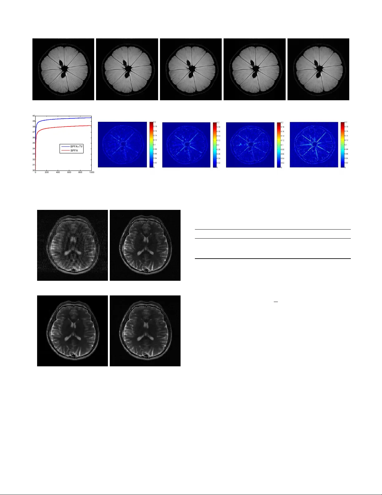
Comments & Academic Discussion
Loading comments...
Leave a Comment