Bayes and Frequentism: a Particle Physicists perspective
In almost every scientific field, an experiment involves collecting data and then analysing it. The analysis stage will often consist in trying to extract some physical parameter and estimating its uncertainty; this is known as Parameter Determinatio…
Authors: Louis Lyons
No v em b er 27, 2024 BA YES AND FREQUENTISM: A P AR TICLE PHYSICIST’S PERSPECTIVE 1 Louis Ly ons Blackett L ab., Imp erial Col le ge, L ondon SW7 2BW, UK and Particle Physics, Oxfor d O X1 3RH e-mail: l .lyons@ph ysics.o x.ac.uk Abstract In almost ev ery scientific field, an experiment in v olv es collecting data and then analysing it. The analysis stage will often consist in trying to extract some ph ysical parameter and estimating its uncertaint y; this is kno wn as Parameter Determination. An example would b e the determi- nation of the mass of the top quark, from data collected from high energy proton-proton collisions. A different aim is to choose b et w een tw o p ossi- ble hypotheses. F or example, are data on the recession sp eed s of distant galaxies prop ortional to their distance d , or do they fit b etter to a mo del where the expansion of the Universe is accelerating? There are t w o fundamen tal approac hes to suc h statistical analyses - Ba yesian and F requen tist. This article discusses the wa y they differ in their approac h to probability , and then goes on to consider ho w this affects the w a y they deal with P arameter Determination and Hypothesis T esting. The examples are taken from every-da y life and from Particle Physics. 1 INTR ODUCTION There are tw o fundamental approaches to statistical analysis, Bay esianism and F requentism. The Bay esian approach dates bac k to Reverend Thomas Bay es, whose paper w as publishes posthumously in 1763. The P olish statistician Jerzey Neyman pla y ed a crucial role in the developmen t of frequentist statistics. In the past there hav e b een vigorous discussions ab out the relative merits of these tw o metho ds (see fig. 2). In this article, the fundamental differences b et w een these t wo approach es will b e explained, and illustrated with examples from Physics and from every-da y life. W e consider them in situations where we are trying to measure a parameter (e.g. the mass of the top quark), or are testing hypotheses (e.g. do we hav e evidence for the existence of the Higgs b oson?) 1 T o appear in Contemporary Physics Figure 1: The Reverend Ba y es (left), whose pap er on his theorem w as published p osth umously in 1763; and Jerzy Neyman, a Polish statistician who play ed a crucial role in the developmen t of the frequentist approach. 1.1 Wh y the fuss? Giv en that there are these fundamentally differen t wa ys of analysing data, how is it p ossible that man y scien tists spend a lifetime measuring all sorts of physical parameters, without b eing a w are of the sharp differences of philosoph y b etw een the Bay esian and F requen tist approaches? The answ er is that in the simplest of problems the t wo metho ds (and others too, lik e χ 2 or maximum likelihoo d) can giv e the identical answ er, that the probability that a parameter µ lies in the range µ l to µ u is, say , 68%. By the ‘simplest of problems’, we mean that the measured v alue m is Gaussian distributed ab out the true v alue µ with kno wn v ariance σ 2 , and that µ can in principle ha ve any v alue from minus infinity to plus infinity . Ho w ev er, in many practical problems in P article Physics, these conditions are not satisfied. The parameter may b e restricted in range (masses cannot b e negativ e), and the data distribution may not b e Gaussian (counting exp er- imen ts often follow the Poisson distribution). So there is ample opp ortunity 2 Figure 2: This incident from the W old Cup so ccer final in 2006 was used to il- lustrate the ‘discussions’ that to ok place b et ween sub-groups within a particular exp erimen t ab out the relative merits of Bay esian and F requen tist analyses[1]. for the results of Ba yesian and frequen tist analyses to differ. The t wo types of statisticians hav e often had strong criticisms of each other’s approach. 1.2 Probabilit y The differences b etw een the Bay esians and F requentists start with their in- terpretation of ‘probabilit y’. Underpinning b oth of these is the mathematical approac h, which is largely due to Russian mathematicians such as Kolmagorov. It is based on axioms (e.g. probabilit y is a n um b er in the range 0 to 1; the sum of the probabilities for something to occur and for it not to o ccur is 1; etc.). This is v ery important for manipulating probabilities, but pro vides little ph ysical in tuition ab out the concept. F or frequen tists, the probabilit y p of ‘something’ is defined in terms of a large n um b er N of essen tially identical, indep enden t trials: if the specified ‘something’ happ ens in s of these trials, p is defined as the limit of the ratio s/ N , as N tends 3 to infinit y . Thus the probabilit y of the sum of the n umbers on t wo rolled dice adding up to 10 can b e determined in this wa y to b e 1/12. Ba y esians attack this definition, as it requires a large num ber of ‘essen tially iden tical’ trials. They claim that to determine whether the trials are indeed ‘es- sen tially indentical’ requires the concept of probability , and hence the definition is circular. Giv en that a rep eated series of trials is required, frequen tists are unable to assign probabilities to single even ts. Th us, with regard to whether it w as raining in Manchester y esterda y , there is no wa y of creating a large num b er of ‘yesterda ys’ in order to determine the probability . F requentists would say that, ev en though they migh t not kno w, in actual fact it either w as raining or it wasn’t, and so this is not a matter for assigning a probability . And the same remains true even if we replace ‘Manchester’ by ‘the Sahara Desert’. Another example would b e the unwillingness of a frequentist to assign a probabilit y to the statement that ‘the first astronaut to set fo ot on Mars will return to Earth aliv e.’ This do es not mean it is an uninteresting question, esp ecially if y ou hav e b een c hosen to be on the first manned-mission to Mars, but then, don’t ask a frequentist to assess the probability . A different type of example inv olves physical constants. F requentists will also not assign probabilities to statements inv olving the numerical v alues of ph ysical parameters e.g Do es dark matter constitute more than 25% of the the critical density for our Univ erse? This again is a situation which cannot b e c hec k ed b y replicated tests. And again, it is either true or false, and not suitable for frequentist probabilities. A similar argumen t applies to statements ab out theories: a F requentist will not allo w probability assignments as to whether the Higgs b oson exists. Ba y esians ha ve a v ery differen t approac h. F or them, probabilit y is a personal assessmen t of how likely they think something is to b e true. It dep ends on their o wn judgement and/or previous knowledge ab out the situation, and can hence v ary from p erson to p erson. Thus if I toss a coin, and ask you what is the probabilit y of the result b eing heads, you are likely to say 50%. But maybe I cheated and looked at the coin, and saw that it was tails, so for me the probabilit y of heads is 0%. Or maybe I just ga ve it a quick glance, and think (but am not certain) that it was tails, so I ass ign a probability of 20% to heads. Because Ba y esians hav e this p ersonal view of probability , they would b e prepared to give numerical estimates for ‘one-off ’ situations (e.g. who gets this y ear’s Nob el Prize?), for parameter v alues (e.g. fraction of dark matter), or concerning theories (e.g. existence of Higgs b oson). Again, these n umerical assessmen ts could v ary from p erson to p erson. 4 PERSONAL PROBABILITIES This is a story I originally heard from Nob el Prize winner F rank Wilczek in a slightly different context, but it illustrates the wa y that for Ba y esians the assessment of probability can differ from p erson to p erson. A sh y p ostdo c is attending a workshop on the topic of ‘Extra Dimen- sions’. Eac h evening, after an intensiv e day’s work, he go es to the lo cal bar, sits next to an empty chair and orders tw o glasses of wine, one for himself and the other for the empty chair. By the third evening, the barman’s curiosity cannot b e controlled and he asks the p ostdo c why he alw a ys orders the extra glass of wine. ‘I w ork on the theory of ex- tra dimensions’, explains the p ostdo c, ‘and it is possible that there are b eautiful girls out there in 12 dimensions, and maybe by quantum me- c hanical tunneling they migh t app ear in our 3-dimensional w orld, and p erhaps one of them might materialise on this empty chair, and I would b e the first p erson talking to her, and then she migh t go out with me’. ‘Y es’, says the barman, ‘but there are three very attractive real girls sitting ov er there on the other side of this bar. Wh y don’t y ou go and ask them if they w ould go out with y ou?’ ‘There’s no p oint’, replies the p ostdo c, ‘that would b e very unlikely .’ It sounds as if this is very p ersonal and not conducive to n umerical estimates. But Ba y esians’ assessmen t of probabilit y should b e consisten t with the ‘fair b et’ concept. If a Bay esian b elieves that a certain statement has a 10% probabilit y of b eing true, they should b e prepared to offer o dds of 9 to 1 (or 1 to 9) to someone who is prepared to b et with them on this being true (or false, respectively). With a p o or assessment of the probability , they would b e in danger of losing money . 2 LIKELIHOODS, BA YES THEOREM AND PRI- ORS W e now ha v e a relev ant digression in to considering likelihoo d functions, and then introduce Bay es Theorem and Priors, essential ingredients of the Bay esian approac h. 2.1 Lik eliho o ds The likelihoo d approach is a v ery p ow erful one for parameter determination, and is also very m uch in v olv ed in Bay esian and F requen tist metho ds for this. Lik eliho o d ratios are also used for c hec king which of tw o theories provides a b etter description of the data. The likelihoo d function is b est illustrated by a simple example. Imagine we are performing a counting exp erimen t for some fairly rare pro cess. F or example. w e may be interested in the flux µ of cosmic ray sho wers with energies ab ov e 5 10 20 electron v olts. W e ha v e a large detector of kno wn area, and find n 0 high energy show ers (e.g. 2) when running the detector for one year. W e wan t to mak e a statement ab out the v alue of the actual flux µ and its uncertaint y . Assuming these cosmic rays are falling on earth at a constant rate, and are indep endent of eac h other, if the true rate is µ , the conditional probabilit y P ( n | µ ) of obtaining n counts is given by the Poisson distribution as P ( n | µ ) = e − µ µ n /n ! (1) Then the lik eliho o d is defined by replacing n in the abov e formula b y the ob- serv ed v alue n 0 . i.e. L ( µ | n 0 ) = e − µ µ n 0 /n 0 ! (2) This likelihoo d is regarded as a function of µ , for the fixed data v alue n 0 . (F or example, if we observ e 2 ev en ts, the likelihoo d is µ 2 e − µ / 2.) It is the probability of observing the data, for different c hoices of µ . Then the likelihoo d estimate of a parameter µ is that which maximises the likelihoo d i.e. It is the v alue of µ whic h maximises the probability of observing the actual data n 0 . (In our case, not surprisingly the lik eliho o d estimate of µ is simply n 0 .) V alues of µ for whic h the likelihoo d is small are regarded as excluded, and the uncertaint y on µ is related to the width of the likelihoo d distribution. A POISSON PUZZLE? According to the Poisson distribution, if the exp ected num ber of ob- serv ations in a specified time is µ , the probabilities P (1 | µ ) and P (2 | µ ) are P (1 | µ ) = µ e − µ , P (2 | µ ) = µ 2 e − µ / 2 F or small µ , these are approximately µ and µ 2 / 2 respectively . Given the fact that the probabilit y for observing one rare ev en t in the time interv al is µ , why is the probability for observing tw o indep endent even ts equal to µ 2 / 2, rather than simply µ 2 , as p erhaps exp ected from eqn. (4)? It is really imp ortant not to confuse the Poisson probabilit y P ( n | µ ) with the lik eliho o d function L ( µ | n 0 ), even though eqns. (1) and (2) bear a remark able similarit y 2 . The distinction should b e easy in this case: P ( n | µ ) is a function of the discrete v ariable n at fixed µ , while L ( µ | n 0 ) is a function of the contin uous v ariable µ at fixed n 0 (see fig. 3). F urthermore, P ( n | µ ) are real probabilities, while the likelihoo d L ( µ | n 0 ) cannot b e interpreted as a probablity densit y (it do es not transform as exp ected for a probability densit y if the parameter is c hosen, for example, as 1 /µ rather than µ ). 2 The ‘!’ symbol in eqns (1) and (2) not only expresses surprise (‘W ow! These equations look very similar), but it also denotes the factorial. 6 µ n 1 2 3 4 Figure 3: Illustration of the difference b et w een the probability density distri- bution for the integer v ariable n and the likelihoo d function for the contin uous parameter µ , for the Poisson distribution (see eqns. (1) and (2)). They inv olve the same function of n and µ , but it is ev aluated at fixed µ for the pd f , but at fixed n for the likelihoo d. 2.2 Ba y es theorem If we consider t wo ‘even ts’ A and B (in the statistical sense), we can write the probabilit y P ( A and B ) of them b oth happ ening as P ( A and B ) = P ( A | B ) P ( B ) (3) where P ( A | B ) is the conditional probability of A happening, given the fact that B has o ccurred. An example could be where we select a random day from last y ear, and A is whether it was sno wy in Oslo, and B that it was a Decem ber day . Then Ba yes Theorem sa ys that the probabilit y of c ho osing a snowy December da y is equal to the probabilit y of it b eing snowy in December, multiplied by 31/365 (the probability of a random day being in December). If the probability of A occuring does not dep end on whether B has done so, eqn. (3) reduces to the b etter-known result that P ( A and B ) = P ( A ) P ( B ) , f or independent A and B (4) CONDITIONAL PROBABILITY Conditional Probabilit y P ( A | B ) is the probability of A , giv en the fact that B has happ ened. F or example, the probabilit y of obtaining a 4 on the throw of a dice is 1/6; but if w e accept only even results, the conditional probability for a 4, given that the num ber is even, is 1/3. 7 Because P ( A and B ) is symmetric in A and B , P ( A and B ) = P ( A | B ) P ( B ) = P ( B | A ) P ( A ) (5) Then Bay es Theorem is derived from the second equality ab ov e: P ( A | B ) = P ( B | A ) P ( B ) /P ( A ) (6) i.e. It relates P ( A | B ) to P ( B | A ). (See section 2.4 for examples where these are ob viously not equal.) It should b e stressed that Bay es Theorem itself is not contro v ersial, and frequen tists are willing to make use of it, provided the v arious probabilities are gen uine frequentist ones. The contro versy b egins when Bay esians replace A by a theoretical parameter (and B is the observed data). The theorem then states that P ( par am | data ) ∝ P ( data | par am ) × P ( par am ) (7) where P ( data | par am ) is just the likelihoo d function; P ( par am ) is the Bay esian prior density , and expresses what was kno wn ab out the parameter b efore our measuremen t; and P ( par am | data ) is the Bay esian p osterior probability density for the parameter, and contains the information ab out the parameter obtained b y com bining the prior information with that from our measurement. BA YESIAN POSTERIORS Jim Berger sa ys that he and his wife hav e professions that are similar, but with a small difference. He is a Bay esian Statistician and she is a fitness trainer. The similarity is that they b oth aim to optimise p oste- riors, but while he wan ts to maximise them, she aims to minimise her clien ts’ p osteriors. The frequentist ob jection to this is that the prior and the posterior both refer to parameter v alues; while this is allow ed for Bay esians, it is strictly forbidden in the frequentist approach. In addition to this, complications are caused by the need to choose a probability density for the prior. 2.3 Ba y esian priors In order to obtain the Bay esian p osterior probability distribution from the like- liho o d function, the latter needs to b e multiplied by the Bay esian prior. There are several fla v ours of Bay esians, who hav e differen t motiv ations for their choice of prior. In this article, we will concen trate on evidence-based priors. So if in our P oisson example of Section 2.1, there was a previous measurement of µ which gav e the result 5 ± 1, the prior might b e chosen as a Gaussian in µ , cen tred on 5 with standard deviation 1 (and probably truncated at zero). Then the p osterior, assuming 2 observed counts, would b e P ( µ | n 0 = 2) = ( µ 2 e − µ / 2) × ( e − ( µ − 5) 2 / 2 / √ 2 π ) , (8) 8 where the first factor on the right is the likelihoo d L ( µ | n 0 = 2), and the second is the prior π ( µ ). This is all v ery w ell when previous data on µ exists. But what if our mea- suremen t is ground-breaking, and essentially nothing is previously known about µ ? How do we now choose the prior π ( µ )? The ‘obvious’ answer is to choose a prior that is indep enden t of µ (but zero for unphysical negative µ ), so as not to fa v our an y particular v alue of µ . Ho w ev er, do w e really believe, as implied by the constant prior, that µ is as likely to b e in the range 10 500 to 10 500 + 0 . 5, as in 0.1 to 0.6? Another problem is that if we are aiming to use a flat prior to express our ignorance ab out a parameter, it is not clear wh y we should c hoose one functional form for the parameter rather than another. F or example, if we are aiming to pro vide a v ery precise measurement of the mass m of the tau neutrino, should w e parametrise our ignorance of its mass b y a flat prior in m , m 2 , ln( m ), etc? Basically priors may b e not bad for parametrising prior knowledge, but are not so go o d for prior ignorance. 2.4 P ( A | B ) 6 = P ( B | A ) Ba y es Theorem relates the conditional probabilities P ( A | B ) and P ( B | A ). Peo- ple often confuse these tw o probabilities, and may erroneously think they are the same. Thus journalists or even Laboratory Spokespersons ma y incorrectly sa y that there is a 99.9% probability that some particle exists, rather than the correct statement that under the null h yp othesis that it do es not, the data are v ery unlik ely . A convincing example of their difference is provided by a database con taining just 2 pieces of information ab out every one on Earth: their sex and whether or not they are pregnant. W e extract a random p erson from the database, who turns out to b e female. Given that the p erson is female, the c hance of b eing pregnan t is ab out 3%. W e then extract another random p erson, who turns out to b e pregnant. Given the fact that the p erson is pregnant, the probability that they are female is 100%. i.e. P ( pr eg nant | f emale ) P ( f emal e | pr eg nant ) (9) Similarly , if you select a card randomly from a deck of 52, the probability of it b eing an ace, if it happ ens to b e a spade, is 1/13; how ev er, the probability of a spade, given that it is an ace, is 1/4. 2.5 A Ba y esian example Imagine that you, a Bay esian, are b etting on the results of coin flips. Each time y ou b et ‘Heads’, and for the first 5 flips it comes do wn ‘T ails’. Given that the probabilit y of b eing wrong 5 times is 3%, should you susp ect it is not a fair coin? W e regard this as a parameter-estimation problem, and wan t to see whether the probability p H of ‘Heads’ is consistent with 0.5. The data (no heads in 5 9 spins) enables us to calculate the likelihoo d function, but in order to extract the posterior probability as a function of p H , we m ust multiply the lik eliho o d b y a prior π ( p H ). Now if the person b etting against us is a complete stranger, w e might assign a constant v alue for p H in the range 0 to 1; then the p osterior is such that p H = 0 . 5 lo oks unlikely . On the other hand, if it is our lo cal village priest, w e are so convinced that he is honest, we use a delta function at p H = 0 . 5, and then ev en if the coin con tin ues to fall down ‘T ails’, we will still b eliev e that it is fair. Thus our conclusion dep ends v ery m uc h on which prior w e c ho ose. Giv en the freedom to select one’s prior, it seems as if Ba y esian in terv als for a parameter can b e very dep endent on this choice. But in some cases, the ‘data o v erwhelms the prior’, and the result b ecomes v ery insensitive to the choice of prior. F or example, the mass of the intermediate vector b oson ( Z 0 ) w as measured at the LEP (Large Electron P ositron) Collider at CERN. The result w as that the lik elihoo d function was essen tially a Gaussian at 91,188 M eV /c 2 , with a width of 2 M eV /c 2 . A Ba yesian no w has to m ultiply this b y the prior probabilit y density for the Z 0 mass. How ever, any reasonable choice of prior will v ary very little ov er the range of a few parts in 10 5 , and so in this case the p osterior is essentially indep endent of the prior. 3 P ARAMETER DETERMINA TION: BA YESIAN APPR OA CH W e illustrate the Ba ysian approac h using a simple example of the determination of the lifetime of some radioactive material. The probability densit y p for a decay at time t is given by p ( t | τ ) = (1 /τ ) e − t/τ (10) where τ is the lifetime we w an t to estimate. W e can estimate τ from a set of deca ys at observed times t i . T o simplify the problem w e assume w e ha ve only one decay at time t 1 (whic h will not give us a very accurate estimate of τ ). The likelihoo d is L ( τ ) = (1 /τ ) e − t 1 /τ , (11) and we ha v e to multiply this b y our choice of prior for τ , to obtain the p osterior p ( τ | t 1 ) = L ( τ ) π ( τ ). As usual, there is a choice for π ( τ ) of an evidence-based prior derived from a previous measurement (in whic h case our p osterior and the resulting range for τ will b e based not only on our measurement, but also on the previous one), ignorance, theoretical motiv ation, etc. Because in man y cases the c hoice of prior is not unique, Bay esian analyses are supp osed to present results for several plausible priors, so as to inv estigate the sensitivit y of the result to the choice of prior. Once the p osterior is av ailable, several options are av ailable for determining a range of preferred τ v alues at some chosen probability level γ , i.e. Z τ u τ l p ( τ | t 1 ) d τ = γ . (12) 10 P ossibilities include: • A central range from τ l to τ u could b e obtained by having probabilities of (1 − γ ) / 2 b elow the range, and (1 − γ ) / 2 ab ov e it. • The upper limit τ U L is obtained b y setting the limits of in tegration in eqn. (12) from zero to τ U L . • In a similar manner, a low er limit τ LL is obtained, using in tegration limits τ LL and infinity . • The shortest p osterior range in τ containing probabability γ is also p opu- lar, but does not corresp ond to the shortest range in the decay rate 1 /τ , or for other reparametrisations of the v ariable of interest. 4 P ARAMETER DETERMINA TION: FREQUEN- TIST APPR OA CH W e no w consider the frequentist approac h for the same problem as in the pre- vious section. The Neyman construction is used to show on a plot of the parameter τ v ersus the data t the likely v alues of t for each τ (see fig. 4(a)). This is ac hiev ed b y using p ( t | τ ) of eqn. (10) for a given τ to select a region of t such that the in tegral of p ( t | τ ) o v er this range of t is, say , 68% 3 ; an example is denoted by the horizon tal line in the figure. By rep eating this pro cedure for all τ , we obtain the ‘confidence band’. In our example, the edges of the band are defined by the straight lines t = 0 . 17 τ and t = 1 . 8 τ . Finally we use the actual observed v alue t 1 to read off the range of τ v alues ( τ l to τ u , which are t 1 / 1 . 8 and t 1 / 0 . 17 rep ectiv ely) for which t 1 is a likely observ ation. F or larger v alues of τ , t 1 is to o small to b e likely , and similarly for smaller τ , t 1 is to o large. In a more plausible scenario where the data consisted of a set of observed deca y times t i , the data statistic could b e the mean of the t i . Then the con- fidence band would be narrow er than in figure, and the range of acceptable τ v alues would b e shorter. An imp ortant feature of this construction is that it do es not require a prior distribution for τ , th us av oiding the p ossible ambiguit y that that w ould hav e in tro duced. Another p oint to note is that the frequentist approac h do es not claim that the range τ l to τ u is probable. Nor do es it make an y statemen t about differen t v alues within this range; it is merely that this is the range of τ v alues for which the observed data is likely (at the chosen confidence level). Fig. 4(b) sho ws a more interesting example. An experiment aims to measure the temp erature T of the fusion reactor at the centre of the sun, by using a 3 This definition do es not pro vide a unique range. The one w e sho w has a probability of 16% on either side of the shaded region, whic h is then known as a central interv al. An alternativ e would b e to hav e the whole of the 32% on the left hand side of the confidence interv al; this would b e useful for pro ducing upp er limits on τ . 11 (a) (b) t= 0 .17 τ u T T u T l t= 1.8 τ l t 1 t ø obs ø Figure 4: The Neyman construction. (a) F or the exponential parameter τ , the cen tral confidence band b etw een the lines t = 0 . 17 τ and t = 1 . 8 τ gives the likely v alues (at the 68% level) of t for each τ . Then a v ertical line at the observed t 1 in tersects the edges of the confidence band at τ l and τ u , and these define the frequen tist range for τ . (b) Here the theory parameter is the temp erature T at the centre of the sun, and the data φ is the measured flux of solar neutrinos, both in arbitrary units. A measurement of the flux φ obs determines a range of temp eratures ( T l to T u ) at the sun’s centre. mon th’s running of a solar neutrino detector to estimate the neutrino flux φ from the sun. Assuming we know all about fusion pro cesses and con v ection in the sun, the prop erties of neutrinos, the p erformance of our detectors, etc, we can construct at each T a region in φ suc h that there is a 68% probability the exp erimen tal result w ould lie in it. Then we use the actual measured flux φ obs to determine the accepted range for T . 4.1 Co v erage F or rep etitions of an exp erimen t using a particular statistical analysis to de- termine a range for the parameter of interest, where the data sets differ from eac h other just by statistical fluctuations, the cov erage is the fraction of the parameter’s in terv als that contain the true v alue of the parameter. This can b e determined from Mon te Carlo simulation, or in some simple cases analytically . Co v erage is a prop erty of the statistical tec hnique that is used to construct the 12 in terv als, and do es not apply to a single measurement. T echniques for whic h the cov erage is equal to the nominal v alue (e.g. 68%) for all v alues of the parameter are said to hav e exact cov erage. If the co verage drops b elow the nominal v alue, the metho d is said to under-co ver. F requentist regard this as bad: if the actual cov erage for determining the parameter is only 30% rather than the nominal 68%, just quoting the range for the parameter as determined by that method is lik ely to mislead a reader into b elieving that y our result is more accurate than it really is. Ov er-co v erage do es not ha v e this problem, but it suggests that maybe the confidence in terv als pro duced b y that metho d are more conserv ativ e (i.e. wider) than they need b e. A particularly imp ortant property of the Neyman construction is that the confidence interv als for the parameter hav e the property of not underco v ering. This prop erty is not guaran teed for other techniques (e.g. Ba yesian, χ 2 , maxi- m um lik eliho o d, metho d of moments). Figure 5: Co verage C for Poisson parameter interv als, as determined by the ∆(ln( L )) = 0 . 5 rule. Rep eated trials (all using the same P oisson parameter µ ) yield different v alues of the observ ation n , each resulting in a range µ l to µ u for µ ; then C is the fraction of trials that give ranges which include the v alue of µ c hosen for the trials. The cov erage C v aries with µ , and has discon tin uities b ecause the data n can take on only discrete integer v alues. F or large µ , C seems to approach the exp ected 0.68. Fig. 5 shows the cov erage C for the follo wing situation. An exp erimen t is p erformed to determine the rate µ of some Poisson counting exp eriment, 13 and n coun ts are observed. The statistical pro cedure c hosen for determining a 68% range for µ is the likelihoo d metho d with the ∆( l nL ) = 0 . 5 rule to define the ends of the range. In en visaged rep etitions of the experiment, n will v ary according to a Poisson distribution with mean µ 0 . Then C ( µ 0 ) is the fraction of the resulting ranges for µ which include µ 0 . The likelihoo d method do es not hav e the frequentist guaran tee of co v erage, and indeed large under- and o v er-co v erage o ccur, e specially at low µ [2]. 5 P ARAMETER DETERMINA TION: COMMON ISSUES Here we discuss some issues that are common to b oth F requen tist and Ba y esian approac hes. 5.1 P arameters with limited range V ery often a physical parameter has meaning only o v er a limited range. F or example, the square of the mass of the neutrino ( m 2 ν ) pro duced in nuclear b eta deca y cannot b e negativ e, the branc hing ratio for some particular decay mo de of an elemen tary particle m ust b e betw een zero and one, etc. Bay esians can incorp orate this information by setting the prior for the parameter to zero in the non-physical region. This ensures that the b est estimate of a parameter or an upp er limit for it are guaran teed to b e physical. In contrast, a frequentist upp er limit could well turn out to be unphysical, or the range for m 2 ν could b e empt y (i.e. there was no ph ysical v alue of m 2 ν for which the data w as likely); in general Particle Physicists are unhappy with such a situation. F or man y years, exp eriments estimating m 2 ν had ‘lik eliho o d functions’ that maximised at negative v alues. Upp er limits for m 2 ν w ere then usually derived b y Ba y esian metho ds. 5.2 In terpretation of µ u ≥ µ ≥ µ l Both Ba y esian and F requentist metho ds of parameter determination end up with a statement of the form µ u ≥ µ ≥ µ l at some probability level, but their in terpretations are very different. F or frequentists, the parameter µ is unknown, but it do es hav e a true v alue and, as discussed earlier, it is not suitable for probability statements. So the probabilit y refers to the range µ l to µ u . If the exp eriment were to b e rep eated man y times, a series of ranges for µ would b e obtained, and the probability refers to what fraction of these ranges contain the true v alue; this is just the co v erage men tioned in Section 4.1. Thus frequentists regard the ends of the range as random v ariables. F or Bay esians, µ u and µ l ha v e b een detemined b y the exp erimental analysis, and are considered fixed; Bay esians do not w an t to b e inv olved in deciding what w ould ha v e happened in h ypothetical rep etitions of the experiment. But they 14 T able 1: Interpretations of “ µ u ≥ µ ≥ µ l at 68% confidence level” Ba y es F requentist What is fixed? µ u , µ l µ What is v ariable? µ µ u , µ l What do es 68% proba- bilit y apply to? Single measuremen t: p ercentage of µ ’s p osterior in range Set of measurements: p ercentage of ranges µ l → µ u that contain µ are prepared to treat the unknown physical constan t as if it w ere a random v ariable, and for them the probability refers to the fraction of the Bay esian p osterior probability density for µ is within the quoted range. 5.3 Dealing with systematics V ery often, in trying to estimate a parameter, some other quantit y in volv ed in the analysis is not known exactly , and this can affect the deduced range for the parameter of in terest. F or example, in the original Reines and Cow an ex- p erimen t [3] to discov er the electron neutrino, a detector sensitive to neutrinos in teracting in it w as built close to a pow erful n uclear reactor. Ho w ev er, there w ere also bac kground processes whic h mimic the in teractions of the reactor neu- trinos. Then the observed n um ber of counts n is likely to be Poisson distributed with mean b + s : P ( n ) = e − ( b + s ) ( b + s ) n /n ! (13) where b is the exp ected background, and s is the signal rate. If b is precisely kno wn, s is the only unknown parameter, and can b e determined essentially as describ ed earlier. But if there is some uncertaint y in the exp ected v alue of b , this results in a systematic uncertaint y in the answer. Statisticians refer to b as a nuisance parameter. Ba y esians tend to treat all parameters (i.e. those of physical interest and n uisance parameters) in a similar manner. Th us, assuming that the background b has b een estimated in a subsidiary counting experiment as m 0 while the result of the main measurement of s + b w as n 0 , they would start by writing the lik eliho o d for s and b as L ( s, b | n 0 , m 0 ) = ( e − ( s + b ) ( s + b ) n 0 /n 0 !) × ( e − b b m 0 /m 0 !) (14) Next this is multiplied b y the c hosen prior π ( s, b ) for s and b , to giv e the p osterior probabilit y p ( s, b ) for the parameter of interest s and the nuisance parameter for the background b . Then this is in tegrated (or ‘marginalised’) ov er b to give the probability density just for the parameter of interest: p ( s ) = Z p ( s, b ) d b (15) 15 Finally the required parameter range is extracted from p ( s ) e.g. a central 68% range. In contrast, frequentists start from the probability densit y p ( n, m | s, b ) for observing any n and m as p ( n, m | s, b ) = ( e − ( s + b ) ( s + b ) n /n !)) × ( e − b b m /m !) (16) The fully frequen tist metho d consists in p erforming a Neyman construction to pro duce a confidence b elt for likely data ( n, m ) as a function of the parameters ( s, b ). In analogy with the simpler problems discussed earlier, the actual data ( n 0 , m 0 ) is then used to read off the region in parameter space ( s, b ) for whic h the data is likely . If a range just for s is desired, it could b e tak en as the extrema of the ( s, b ) region, although this will give rise to ov erco v erage. There are also v arious appro ximate metho ds, which are simpler than the full Neyman construction and which tend to pro duce less o v erco v erage (but for whic h the frequentist guarantee of cov erage no longer applies). An example is the profile likelihoo d approach, in which the probability p ( n, m | s, b ) is replaced b y p prof ( n, m | s, b best ( s )), where b best ( s ) is the v alue of b whic h maximises the probabilit y for that v alue of s ; b ecause b best ( s ) is a function of s , the profiled probabilit y dep ends on the single parameter s , which simplifies the problem. PR OFILE LIKELIHOOD In many situations, the probability of observing a particular set of data d dep ends not only on a parameter of physical interest φ (e.g. the mass of the Higgs b oson), but also on some other so-called n uisance parameters ν (e.g. a scale factor for correcting jet energies as measured in the detector). Then the likelihoo d L ( φ, ν | d ) is a function of b oth sets of parameters φ and ν . In order to draw conclusions ab out φ , it is ofter helpful to consider the profile lik elihoo d L prof ( φ, ν max ( φ ) | d ), where for eac h v alue of φ , the nuisance parameters are chosen to maximise the full likelihoo d L ( φ, ν | d ), i.e. ν max v aries with φ . How ev er, L prof no w is a function just of φ but not of the nuisance parameters ν , thereb y simplifying the problem of making inferences ab out the parameter of in terest φ , at the cost of losing some of the prop erties of the lik eliho o d function. Rather than maximising L with resp ect to ν , Bay esian methods tend to marginalise , i.e. integrate the lik eliho o d with resp ect to ν , usu- ally after using priors for ν , to conv ert L into a p osterior probability distribution for φ . F or the case where L is a multi-dimensional Gaussian distribution such as L ∝ exp {− ( aφ 2 + 2 bφν + cν 2 ) } , marginalisation o v er ν or profiling with resp ect to it will give the same functional form for the mo dified likelihoo ds. Ref. [4] contains a longer discussion of systematics, while Demortier[5] deals 16 with wa ys of incorp orating systematics in b oth parameter determination and h yp othesis testing. 6 HYPOTHESIS TESTING P ossibly more interesting than Parameter Determination is Hyp othesis T esting. Here the issue is to decide whic h of tw o (or more) comp eting theories pro vides a b etter fit to some data. F or example, was data collected at the Large Hadron Collider at CERN in the first half of 2012 more consistent with what is kno wn as the Standard Mo del (S.M.) of P article Ph ysics without an ything new, or with the pro duction of the Higgs b oson in addition to the known S.M. pro cesses? (See fig. 6) Figure 6: The observ ed distribution in the CMS exp eriment for the effective mass m γ γ of pairs of γ s pro duced in high energy proton-proton collisions at CERN’s LHC. If the Higgs boson exists and deca ys to a pair of γ s, it could result in a p eak centred on the mass of the Higgs. Otherwise, the expected distribution is expected to b e smooth. In the main plot, the ev en ts are weigh ted according to their qualit y; the inset sho ws un w eigh ted ev ents. The apparen t p eak around 125 GeV is part of the evidence for the existence of a new particle, whose prop erties seem consisten t with those exp ected for a Higgs b oson. In Particle Physics, for reasons to b e explained b elow, it is muc h more com- 17 mon to use a frequentist metho d to decide. In other fields, Bay esian approac hes tend to b e fav oured. W e discuss Bay esian metho ds briefly in section 7. 6.1 F requentist approac h The first task is to choose some data statistic t whic h will help distinguish b et w een the hypotheses. In the simple case of a counting exp erimen t, where the data consists just of the num ber of accumulated counts n 0 for a giv en amount of running time, it could simply b e n 0 . Then in most cases new physics would manifest itself in a larger num ber of counts when the exp ected rate is s + b , than if there were just background; here s and b are the exp ected signal and bac kground rates resp ectively . In more complicated cases, the data could consist of one or more histograms or m ulti-dimensional distributions. Then usually t is chosen as a lik elihoo d ratio for the data, assuming the tw o hypotheses: t = L 1 ( H 1 | d ) /L 0 ( H 0 | d ) (17) where L 1 is the lik eliho o d for H 1 (the hypothesis of signal + background), giv en the data, while L 0 is for the background only hypothesis H 0 , given the same data. When the hypotheses are completely sp ecified without any free parameters, they are kno wn as ‘simple h ypotheses’ and the abov e form ulation is satisfactory . Then the Neyman-P earson lemma[6] sa ys that if we choose H 0 based on the likelihoo d ratio b eing b elow some suitably defined cut-off, this will guaran tee that we will ac hieve the lo west rate for “Errors of the Second Kind” (i.e.incorrectly selecting H 0 when H 1 is true), for a given rate for “Errors of the First Kind” (i.e. rejecting H 0 when it is true ). If, ho w ev er, one or more of the hypotheses in v olv es free parameters (‘com- p osite h yp otheses’), the Neyman-Pearson lemma does not apply . Nevertheless a form of the likelihoo d ratio, suc h as the ratio of profile likelihoo ds, is often used as a metho d that may well b e nearly optimal. 6.2 p -v alues F or the null h yp othesis H 0 , the exp ected distribution of our test statistic t is f 0 ( t ). Then for a given observed v alue t obs , the p -v alue is the fractional area in the tail of f 0 ( t ) for t greater than or equal to t obs . F or definiteness we consider the single-sided upp er tail (assuming that the alternative hypothesis yields larger v alues of t obs ), but low er or 2-sided tails could b e appropriate in other cases . A small p -v alue means that the data are not very consistent with the hy- p othesis. Apart from the p ossibility that the cause of the discrepancy is new ph ysics, it could b e due to an unlik ely statistical fluctuation, an incorrect imple- men tation of the hypothesis being tested, an inaccurate allow ance for detector effects, etc. As more and more data are acquired, it is p ossible that a small (and perhaps not physically significan t) deviation from the tested null h yp othesis could result 18 in the p 0 b ecoming small as the data b ecome sensitive to the small deviation. F or example, a set of particle decays may b e exp ected to follow an exp onential distribution, but there might b e a small background characterised b y decays at v ery short times, and which is not allow ed for in the analysis. A small amount of data might be insensitive to this background, whereas a large amoun t of data migh t giv e a very small p -v alue for a test of exp onen tial deca y , even though the bac kground is fairly insignificant. With enough data, we ma y b e able to include ph ysically motiv ated corrections to our naiv e H 0 . The possibility of a statisti- cally significant but physically unimp ortant deviation has b een mentioned by Co x[7]. It is extremely imp ortant to realise that a p -v alue is the probabilit y of ob- serving data lik e that observ ed or more extreme, assuming the hypothesis is correct. It is not the probabilit y of the h yp othesis being true, given the data. These are not the same - see section 2.4. Man y of the negativ e comments ab out p -v alues are based on the ease of misin terpreting them. Thus it is p ossible to find statemen ts that of all exp eri- men ts quoting p -v alues b elow 5%, and which thus reject H 0 , man y more than 5% are wrong (i.e H 0 is actually true). In fact, the expected fraction of these exp erimen ts for whic h H 0 is true depends on other factors, and could take on an y v alue b etw een zero and unity , without in v alidating the p -v alue calculation. 6.3 p -v alues for t w o h yp otheses With tw o hypotheses H 0 and H 1 , we can define a p -v alue for eac h of them. W e adopt the con v en tion that H 1 results in larger v alues for the statistic t than do es H 0 . Then p 0 is defined as the upp er tail of f 0 ( t ), the probability densit y function ( pd f ) for observing a measured v alue t when H 0 is true. It is con v en tional to define p 1 b y the area in the lo wer tail of f 1 ( t ) (i.e to w ards the H 0 distribution) – see Fig. 7(b), which shows the probabilit y densities for obtaining a v alue t of a data statistic, for hypotheses H 0 and H 1 . F or a sp ecific v alue t obs , the p -v alues p 0 and p 1 corresp ond to the tail areas ab o v e t obs for the H 0 pd f , and b elow t obs for H 1 , resp ectively . 4 Then t crit is the critical v alue of t suc h that its p 0 v alue is equal to a preset level α for rejecting the n ull hypothesis. The p 1 -v alue when t = t crit is denoted by β , and the p ow er of the test is 1 − β . The p ow er is the probability that we successfully reject the null h yp othesis, assuming that the alternative is true. W e exp ect the p ow er to increase as the signal strength in H 1 b ecomes stronger, and the pd f s for H 0 and H 1 b ecome more separated. Dep ending on the separation of the t wo pd f s and on the v alue of the data statistic t , several situations are now p ossible (see T able 2): • p 1 is small, but p 0 acceptable. Then we accept H 0 and reject H 1 . i.e. we exclude the alternative hypothesis. 4 If t is a discrete v ariable, such as a num b er of even ts, then ‘ab ov e’ is replaced by ‘greater than or equal to’, and correspondingly for ‘b elow’. 19 (a) (b) (c) H0 H1 p 1 p 0 t t t t 0 t 0 t 0 t 1 H0 H1 Ex clu sio n No de cisi on Disco very t cr it Figure 7: Exp ected distributions for a statistic t for H 0 = background only (solid curves) and for H 1 = background plus signal (dashed curv es). In (a), the signal strength is very w eak, and it is imp ossible to choose b etw een H 0 and H 1 . As shown in (b), whic h is for mo derate signal strength, p 0 is the probabilit y according to H 0 of t b eing equal to or larger than the observed t 0 . T o claim a discov ery , p 0 should b e smaller than some pre-set level α , usually tak en to corresp ond to 5 σ ; t crit is the minimum v alue of t for this to b e so. Similarly p 1 is the probability according to H 1 for t ≤ t 0 . The exclusion region corresp onds to t 0 in the 5% lo w er tail of H 1 . In (b) there is an intermediate “No decision” region. In (c) the signal strength is so large that there is no ambiguit y in choosing b etw een the hypotheses. In order to protect against a down w ard fluctuation in a situation lik e (a) resulting in an exclusion of H 1 when the c urv es are ess en tially identical, C L s is defined as p 1 / (1 − p 0 ) (see Section 6.6). • p 0 is very small, and p 1 acceptable. Then we accept H 1 and reject H 0 . This corresp onds to claiming a discov ery . • Both p 0 and p 1 are acceptable. The data are compatible with b oth hy- p otheses, and we are unable to choose b etw een them. • Both p 0 and p 1 are small. The c hoice of decision is not obvious, but basically b oth hypotheses should b e rejected. 20 5 σ DISCO VER Y, 95% EX CLUSION Searc hes for new phenomena in Particle Ph ysics typically choose the ‘Standard Model’ as the null hypothesis H 0 , and a sp ecific form of New Physics as H 1 . The exc lusion level for H 1 is usually set at 5%, whereas that for rejecting H 0 (and p erhaps claiming the disco v ery of New Physics) is usually ‘5 σ ’, i.e p 0 ≤ 3 × 10 − 7 . Some (not v ery con vincing) reasons for the stringen t criterion for reject- ing H 0 include: • The past history of false discov ery claims at 3 σ and 4 σ lev els. • The p ossibility that systematic effects hav e b een underestimated. • The Lo ok Elsewhere Effect (see Section 6.5). • Subliminal Bay esian reasoning that the Standard Mo del is intrin- sically more likely to b e true than some sp ecific sp eculation ab out New Physics. • The em barrassmen t of having to withdra w a sp ectacular but in- correct claim of discov ering New Physics. In con trast, incorrect exclusion of New Physics is not regarded as so dramatic, and so the weak er criterion of 5% is used. As Glen Co w an has remarked, “If you are lo oking for y our car keys and are 95% sure they are not in the kitchen, it’s a go o d idea to start lo oking somewhere else”[8]. Fig 8(a) illustrates the ( p 0 , p 1 ) plot for defining v arious decision regions. T able 2: Cho osing b etw een tw o hypotheses, based on p 0 and p 1 . p 0 p 1 Result If H 0 true If H 1 true V ery small O.K. Disco v ery Error of 1 st kind Correct choice O.K. Small Exclude H 1 Correct choice Error of 2 nd kind O.K. O.K. Mak e no choice Loss of efficiency Loss of efficiency V ery small Small ? ? ? 6.4 p-v alues or lik eliho o ds? Rather than calculating p -v alues for the v arious hypotheses, we could use their lik eliho o ds L 0 and L 1 . While p -v alues use tail areas b eyond the observed statis- tic, the likelihoo d is simply the heigh t of the pd f at t obs . W e return to lik elihoo d 21 (a) (b) Figure 8: Plots of p 0 against p 1 for comparing a data statistic t with tw o hy- p otheses H 0 and H 1 , whose expected pd f s for t are assumed to b e t w o Gaussians of p eak separation ∆ µ , and of equal width σ (see fig. 7). (a) F or a pair of pd f s with a given separation, the allow ed v alues of ( p 0 , p 1 ) lie on a curve or straight line (sho wn solid in the diagram). As the separation ∆ µ increases, the curv es approac h the p 0 and p 1 axes. Rejection of H 0 is for p 0 less than, say , 3 × 10 − 7 ; here it is shown as 0.05 for ease of visualisation. Similarly exclusion of H 1 is sho wn as p 1 < 0 . 1. Thus the ( p 0 , p 1 ) square is divided in to four regions: the largest rectangle is when there is no decision, the long one ab ov e the p 0 -axis is for exclusion of H 1 , the high one beside the p 1 -axis is for rejection of H 0 , and the smallest rectangle is when the data lie b etw een the tw o pd f s. F or ∆ µ/σ = 3 . 33, there are no v alues of ( p 0 , p 1 ) in the “no decision” region. In the C L s pro cedure, rejection of H 1 is when the statistic t is suc h that ( p 0 , p 1 ) lies below the diagonal dotted straight line. (b) Contours of constant lik eliho o d ratio r = L 0 /L 1 for Gaussian pd f s. The upp er righ t region is inaccessible; the diagonal line from (0,1) to (1,0) corresp onds to the pd f s lying on top of each other i.e. no sen- sitivit y . The diagonal through the origin is when t obs is mid-w a y betw een the t w o pd f s. With larger separation of the Gaussian pd f s and for constant p 0 the lik eliho o d ratio increases. ratios in Section 7. As mentioned in section 6.1, the Neyman-Pearson lemma provides the best w a y of choosing b etw een tw o simple hypotheses, but even when one or b oth 22 h yp otheses contain free parameters, the likelihoo d ratio may w ell b e a suitable statistic for summarising the data and for helping choose b etw een the hypothe- ses. In general, it will b e necessary to generate the expected distributions of the lik elihoo d ratio according to the h yp otheses H 0 and H 1 , in order to mak e some deduction based on the observed likelihoo d ratio; for comp osite hypothe- ses there are of course the complications caused b y the n uisance parameters. The decision process ma y w ell b e based on the p -v alues p 0 and p 1 for the t wo h yp otheses (see fig. 8). In that case, the pro cedure can b e regarded as either a lik eliho o d ratio approac h, with the p -v alues simply pro viding a calibration for the v alue of the likelihoo d ratio; or as a p -v alue metho d, with the likelihoo d ratio merely b eing a conv enien t statistic. 6.5 Lo ok Elsewhere Effect If y ou are pla ying cards, and in y our hand of 13 cards y ou observe that y ou hav e 4 queens, y ou migh t think that that is v ery un usual. Indeed the probabilit y of a random set of 13 cards containing 4 queens is 0.0026. How ever, since you decided that ‘4 queens’ was unusual only after you lo oked at your cards, you migh t hav e b een equally surprised by 4 kings; or 4 jacks; or ace, t w o, three, four of the same suit; etc. T aking these into accoun t, the probability of a surprising hand of cards similar to what we had is going to b e a fair bit larger than 0.0026. A similar effect explains why a seemingly improbable even t in our every-da y life (e.g. a chance meeting with someone we had b een thinking ab out recen tly) ma y in fact b e muc h more likely , if we hav e not decided at the b eginning of the da y that this sp ecific even t would b e a real coincidence if it happ ened. Often in High Energy Physics, we are lo oking for some new phenomenon. Th us we may b e searching for a new particle, whose mass is not pre-defined, in a histogram such as that of fig. 6. When w e observ e an enhancemen t, we can calculate the p -v alue (the chance of observing a statistical fluctuation at least as big as the one in our data, assuming that no such particle in fact exists), at the observ ed mass. But this of course underestimates the c hance of ha ving a fluctuation anywhere in our mass distribution, whic h we migh t mistak enly ascrib e to a new particle. W e th us need to calculate the probabilit y of observing an effect at least as impressiv e as ours, an ywhere in our mass distribution. In P article Ph ysics, this dilution of the significance is known as the Look Elsewhere Effect (LEE). Similar considerations are relev an t for searc hes in other fields. Thus claims for disco v eries of gravitational wa ves would need to calculate the chance of a statistical fluctution mimic king the observ ed effect not only at the observ ed time, frequency and signal structure, but anywhere in the whole dynamic range of these v ariables for which a real signal is p ossible. Of course, sp ecifying where exactly ‘Elsewhere’ is is fraught with am biguities. Th us for the ab ov e example of searching for a new particle, fig. 6 is relev ant for the p ossibility of it decaying to 2 photons, but other deca y m odes could b e p ossible, and hence could b e relev an t to the LEE. Similarly , maybe the particle w e are considering cannot b e pro duced enough at high masses for us to ha v e 23 the chance of detecting it, so the whole mass range is not relev ant for the LEE. The conclusion is that when p -v alues are corrected for the LEE, it is imp ortant to sp ecify exactly what has b een taken into account. 6.6 C L s The C L s metho d[9, 10] w as in tro duced in the LEP exp erimen ts at CERN in searc hes for new particles. When evidence for suc h a particle is not found, the traditional frequen tist approac h is to exclude its production if p 1 is smaller than some preset lev el γ , whic h in Particle Physics is t ypically set at 5%. Ho w ev er, there is then a 5% probability that H 1 could be excluded, ev en if the exp eriment w as such that the H 0 and H 1 pd f s lay on top of each other i.e. there was no sensitivit y to the pro duction of the new phenomenon. T o protect against this, the decision to exclude H 1 is based on p 1 / (1 − p 0 ), kno wn as C L s 5 . It is thus the ratio of the left hand tails of the pd f s for H 1 and H 0 . Fig 8(a) shows a ( p 0 , p 1 ) region for which H 1 is excluded by C L s . The fact that it is clearly smaller than for the standard frequentist exclusion region is the price one has to pa y for the protection it provides against excluding H 1 when an exp eriment has no sensitivity to it. W e regard it as conserv ative frequentist. It is interesting that the C L s exclusion line in fig. 8(a) for the case of tw o Gaussians is identical to that obtained by a Ba y esian pro cedure for determining the upp er limit on µ 1 when the latter is restricted to p ositive v alues, and with a uniform prior for µ 1 . In a similar manner, the standard frequentist pro cedure agrees with the Ba y esian upp er limit when the restriction of µ 1 b eing positive is remov ed. In principle, similar protection against discov ery claims when the experiment has no sensitivit y could b e employ ed, but it is deemed not to be necessary b e- cause of the different levels used for discov ery and for exclusion of H 1 (t ypically 3 × 10 − 7 and 0.05 resp ectively). 6.7 When neither H 0 or H 1 is true It may well b e that neither H 0 nor H 1 is true. With no more information a v ailable, it is of course impossible to say what we expect for the distribution of our test statistic t . On the plot of fig. 8(a), our data ma y fall in the small rectangle next to the origin. It is certainly not true that a small v alue for p 0 necessarily implies that H 1 is correct, although for small enough p 0 , ruling out H 0 is a p ossibility . 7 BA YESIAN METHODS The Bay esian approac h is more naturally suited to making statements ab out what we b elieve ab out t wo (or more) hypotheses in the light of our data. This 5 This stands for ‘confidence level of signal’, but it is a p o or notation, as C L s is in fact a ratio of p -v alues, which is itself not even a p -value, let alone a confidence level. 24 con trasts with Goo dness of Fit, whic h in v olv es considering other p ossible data outcomes, but fo cusses on just one hypothesis. All Bay esian metho ds inv olv e the lik eliho o d function, p ossibly mo dified to tak e in to accoun t n uisance parameters. F or Hyp othesis T esting, some form of a ratio of (modified) likelihoo ds is usually in v olv ed. F or simple h ypotheses, this is just L 0 ( H 0 ) /L 1 ( H 1 ), where L i ( H i ) = p ( x | H i ), the probability (densit y) for observing data x for the h yp othesis H i . The issue is going to b e ho w nuisance parameters 6 ν are dealt with for non-simple hypotheses. F or the likelihoo d ap- proac h (as opp osed to the Ba y esian one, whic h also requires priors), it is usual to profile them i.e. the profile likelihoo d is L i ( H i | ν best ), where ν best is the set of pa- rameters which maximise L . In Particle Ph ysics, the profile likelihoo d approac h is a popular method for incorp orating systematics in parameter determination problems. The complications of applying Bay esian metho ds to mo del selection in prac- tice are due to the choices for appropriate priors. This is particularly so for those parameters whic h occur in the alternative hypothesis H 1 but not in the n ull H 0 . Loredo[11] and T rotta[12] hav e provided reviews of the application of Ba y esian tec hniques in Astrophysics and Cosmology , where their use is more common than in Particle Physics. 7.1 Ba y esian p osterior probabilities When there are no nuisance parameters in v olv ed, the ratio of the posterior probabilities for H i is p post ( H 0 | x ) /p post ( H 1 | x ), where p post ( H i | x ) = L i ( H i ) π i , (18) and π i is the assigned prior probability for h ypothesis i . F or example, the h yp othesis of there being a Higgs boson of mass 110 GeV might w ell be assigned a small prior, in view of the exclusion limits from LEP . With nuisance parameters, the p osterior probabilities b ecome p post ( H i | x ) = Z L i ( H i | ν ) π i ( ν ) π i dν (19) where π i is the prior probability for h yp othesis i and π i ( ν ) is the joint prior for its n uisance parameters. i.e. w e no w ha v e in tegrated ov er the n uisance param- eters. This contrasts with the likelihoo d metho d, where maximisation with resp ect to them is more usual. Even with π i ( ν ) being a constant, integration and maximisation can select differen t regions of parameter space. An example of this would b e a likelihoo d function that has a large narro w spike at small ν , and a broad but low er enhancement at large ν . 6 F or the purp ose of mo del comparison, any parameters are considered as nuisance param- eters, even if they are physically meaningful. e.g. the parameters of a straight line fit, the mass of the Higgs boson, etc. 25 In relation to all Bay esian methods, it is to be emphasised that the c hoice of a constan t prior, esp ecially for m ulti-dimensional ν , is by no means ob vious (compare Section 2.3). V ery often, there are several p ossible choices of v ariable for the nuisance parameters, with none of them b eing obviously more natural or appropriate that the others. Thus a point in 2-dimensional space could b e written as Cartesian ( x, y ) or p olar ( r , θ ); constant priors in the t w o sets of v ariables are differen t. Similarly in fitting data by a straigh t line y = a + b x , using a seemingly inno cuous flat prior for b = tan θ results in angles θ in the range 0 ◦ to 89 ◦ ha v e the same prior probabilit y as those in the range 89 ◦ to 89 . 5 ◦ . It should b e realised that the results for Hyp othesis T esting are more sensi- tiv e to the choice of prior than in parameter determination. Th us in parameter determination, sometimes a prior is used whic h is constant ov er a wide range of ν , and zero outside it. The resulting range for the parameter, as deduced from its p osterior, may well b e insensitive to the range used, provided it includes the region where the lik eliho o d L ( ν ) is significan t. F or comparing h yp otheses, ho w ev er, there can b e parameters which o ccur in one hypothesis but not the other. (An example of this is where H 1 corresp onds to smo oth background plus a p eak, while H 0 is just smooth background.) The widths of such priors affect their normalisation, and hence also the Bay es factor (see next Section) directly . On the other hand, in searc hes for a new particle of unknown mass, the Ba y esian probabilit y for the particle existing will dep end on the range of the prior used for the particle’s mass - the wider the range, the low er the normalisa- tion and hence the low er the probability 7 . A t least qualitatively , this resembles the effect of the LEE in the frequentist approach, where the significance of a p eak in a mass sp ectrum is diluted if the search extends ov er a wide mass range (see s ection 6.5). 7.2 Ba y es factor F or each hypothesis we define R i = p post /π , where p post and π are resp ectively the p osterior and prior probabilities for hypothesis i . Thus R is just the ratio of p osterior and prior probabilities. Then the Bay es factor for the tw o h yp otheses H 0 and H 1 is B 01 = R 0 /R 1 . If the t w o h ypotheses are both simple, then this is just the likelihoo d ratio. If either is comp osite, the relev ant integrals are required for p post . A small v alue of B 01 fa v ours H 1 . Demortier[13] has dra wn atten tion to the fact that it can be useful to cal- culate the minimum Bay es factor[14]. This is defined as ab ov e, but with the extra nuisance parameters of H 1 set at v alues that minimise B 01 , i.e. they are as fa v ourable as p ossible for H 1 . If even this v alue of B 01 suggests that H 1 is not to b e preferred, then it is a waste of time to inv estigate further since an y c hoice of priors for the extra parameters cannot make B 01 smaller. 7 This is an example of Occam’s Razor, whereby a simpler hypothesis may be fav oured o v er a more complex one. 26 T able 3: Cost function. Typically the cost A assigned to a false discov ery claim w ould b e larger than B , the cost for a failure to discov er. There is zero cost for making a correct decision. H 0 true H 1 true Accept H 0 Correct choice. Cost =0 F ailure to discov er. Cost = B Reject H 0 F alse discov ery claim. Cost = A Correct choice. Cost = 0 7.3 Other Ba y esian metho ds The Bay esian approach can b e used in conjunction with Decision Theory , in order to provide a pro cedure for choosing b et w een tw o hypotheses. In addition to any priors, a cost function has to be defined, which assigns a numerical ‘cost’ for each combination of the true hypothesis ( H 0 or H 1 ), and the p ossible decisions - s ee T able 3. The decision pro cedure is designed to minimise the exp ected cost, as determined by the cost function and the exp ected distribution of p osterior probabilities for H 0 and H 1 . Because of the problems of assigning realistic costs, and the use of priors in determining the p osteriors for the h yp otheses, there is little or no usage of this approac h in Particle Physics searches for New Physics. Other Bay esian metho ds such as AIC, BIC,.... (Ak aike Information Cri- terion, Bay es ian Information Criterion,.....) aim to provide appro ximations to the Bay es factor, but which are easier to calculate. Given the p ow erful com- putational facilities av ailable now ada ys, these metho ds are likely to decrease in general usage. Again there is little or no experience of using them in P article Ph ysics applications. 7.4 Wh y p is not equal to the lik eliho o d ratio There is sometimes discussion of why a likelihoo d ratio approach (or the Bay es factor, if there are nuisance parameters) can giv e a very different numerical answ er to a p -v alue calculation. A reason some agreement might b e exp ected is that they are b oth addressing the question of whether there is evidence in the data for new physics. In fact they measure v ery differen t things. Th us p 0 simply measures the consistency with the null h yp othesis, without any regard to the degree of agree- men t with the alternative, while the likelihoo d ratio tak es the alternative into accoun t. There is thus no reason to exp ect them to b ear any particular rela- tionship to each other. This can b e illustrated by contours of constant v alues of the likelihoo d ratio r = L 0 /L 1 on a p 0 v ersus p 1 plot (see fig. 8(b)). The figure is constructed by assuming that the pd f s for the tw o hypotheses H 0 and H 1 are giv en by Gaussian distributions, both of unit width. Then at constant p 0 , it is seen that the likelihoo d ratio can tak e a range of v alues, corresponding to the 27 Gaussians ha ving differen t separations. Thus with the Gaussian for H 0 ’s pd f cen tred at zero, a measured v alue of 5.0 yields a p 0 -v alue of 3 × 10 − 7 , regardless of the p osition of the H 1 Gaussian. Such a small p -v alue is usually taken as sufficien t to reject H 0 . As the centre of the H 1 Gaussian starts at µ 1 = 0, the t w o Gaussian pd f s are identical, and r = 1. With increasing µ 1 , p 0 of course remains constant, but r at first decreases to a minimum when µ 1 = 5, but then increases through unity when µ 1 = 10 (i.e. the data is midwa y b etw een the pd f p eaks), and then keeps on rising with further increases of the separation of the pd f s. At that stage, the data are more in agreement with H 0 than with H 1 , despite the small v alue of p 0 . 8 CONCLUSION T able 4: Comparison of Bay es and F requen tist approaches Ba y es F requentist Basis of metho d Ba y es Theorem → posterior probabilit y distribution Uses pd f for data, for fixed pa- rameter v alues Meaning of proba- bilit y Degree of b elief F requentist definition Probabilit y for pa- rameters? Y es No, no, no Needs prior? Y es No Choice of interv al? Cen tral, upp er limit, shortest,... Choice of ordering rule Data used Only the data you hav e Also other p ossible data Needs ensemble of possible exp eri- men ts? No Y es (but often not explicit) Ob eys the Likeli- ho o d Principle? Y es No Unph ysical/empt y ranges p ossible? Excluded by prior Can o ccur Final statement P osterior prob dist P aram v alues for which data is lik ely Do param ranges co v er? Regarded as unimp ortant Built in Include systematics In tegrate o v er prior Extend dimensionality of fre- quen tist construction W e hav e seen how Bay esians and F requentists differ fundamen tally in the w a y they consider probability . This then affects the wa y they approach the 28 topics of parameter determination, and of choosing b etw een t w o h yp otheses. T able 4 provides a summary of the differences b etw een the tw o approaches. A cynic’s view of the tw o techniques is provided by the quotation: “Ba y esians address the question ev eryone is in terested in by using assump- tions no-one b elieves, while F requentists use imp eccable logic to deal with an issue of no interest to any one.” Ho w ev er, it is not necessary to b e so negative, and for ph ysics analyses at the CERN’s LHC, the aim is, at least for determining parameters and setting upp er limits in searches for v arious new phenomena, to use b oth approaches; similar answ ers w ould strengthen confidence in the results, while differences suggest the need to understand them in terms of the somewhat different questions that the t w o approac hes are asking. It thus seems that the old war b etw een the tw o metho dologies is subsiding, and that they can hop efully live together in fruitful co op eration. A CKNO WLEGEMENTS I would like to thank Bob Cousins, David v an Dyk, Luc Demortier and Rob erto T rotta for their advice on v arious sections of this article. References [1] V. Lubicz, “Extraction of α from B → π π decays”, T alk at the Nagoy a Conference on the CKM unitary triangle (2006). [2] J. G. Heinrich, “Cov erage of Error Bars for Poisson Data”, http://www- cdf.fnal.gov/physics/statistics/notes/cdf6438_ coverage.pdf . [3] C. L. Cow an et al, Science 124 (1956) 103. [4] J. G. Heinrich and L. Lyons, Annual Review of Nuclear and Particle Science 57 (2007) 145. [5] L. Demortier, Pro ceedings of PHYST A T 2007, CERN-2008-001, p. 23 [6] J. Neyman and E. S. P earson, Phil T rans. Ro y al Soc. London A 231 (1933) 289. [7] D. Co x, ‘Some problems connected with statistical inference’, Annals of Mathematical Statistics 29 (1958)357. [8] Remark b y G. Co w an at Conference on ‘Adv anced Statistical T echniques in Particle Physics’, IPPP/02/78 (Durham, 2002). [9] A. Read, ‘Mo dified frequen tist analysis of searc h results’ in W orkshop on Confidence Limits, CERN Y ellow Report 2000-05, page 81; ‘Presentation of search results - the C L s metho d’, in ‘Adv anced Statistical T echniques in P article Ph ysics’, Durham IPPP/02/39 (2002) page 11. 29 [10] T. Junk, ‘Sensitivit y , exclusion and discov ery with small signals, large bac kgrounds and large systematic uncertainties’, CDF note CDF/DOC/ST A TISTICS/PUBLIC/8128 (2007), http://www- cdf.fnal. gov/ ~ trj/mclimit/mclimit_csm.pdf [11] T. J. Loredo, ‘F rom Laplace to Sup ernov a SN1987a: Ba y esian inference in Astrophysics’, in ‘Maximum Entrop y and Bay esian Metho ds’ (Kluw er Academic Publishers, 1990), p81. [12] R. T rotta, ‘Ba y es in the sky: Ba y esian inference and mo del selection in Cosmology’, Contemporary Physics 49 (2008) 71. [13] L. Demortier, priv ate comunication. [14] W. Edwards, H. Lindman and L. J. Sa v age, “Bay esian statistical inference for psychological research,” Psychol. Rev. 70 (1963) 193. 30
Original Paper
Loading high-quality paper...
Comments & Academic Discussion
Loading comments...
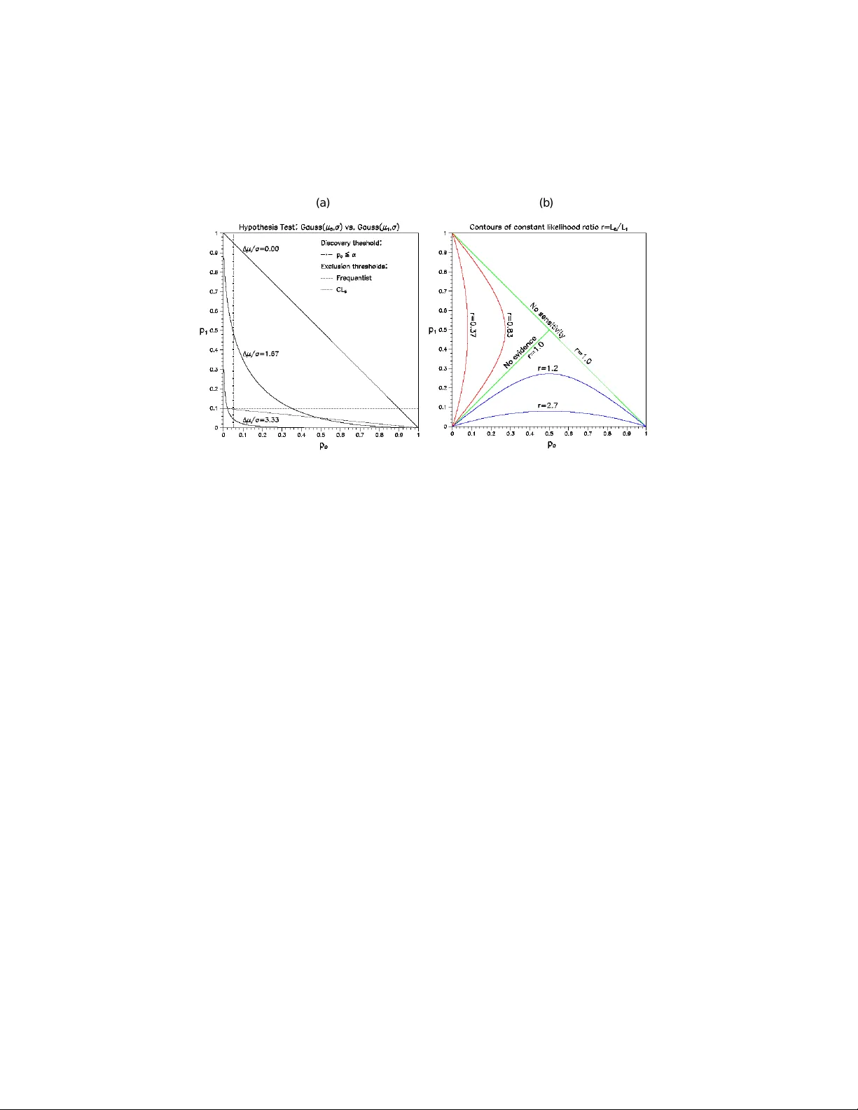
Leave a Comment