Astroinformatics of galaxies and quasars: a new general method for photometric redshifts estimation

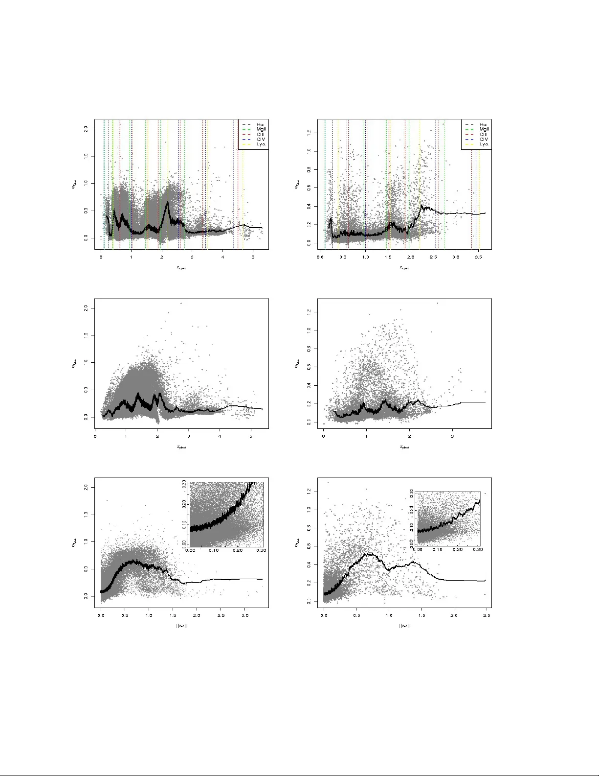
Mon. Not. R. Astron. Soc. 000 , 1–36 (2002) Printed 3 Novem ber 2021 (MN L A T E X style ﬁle v2.2) Astroinformatics of galaxies and quasars: a new general metho d for photometric redshifts estimation O. Laurino 1 , 2 ? , R. D’Abrusco 2 , G. Longo 3 , 4 and G. Riccio 3 1 Astr onomic al Observatory of T rieste - INAF, T rieste, Italy 2 Harvar d-Smithsonian Center for Astr ophysics - Cambridge (MA), US 3 Dep artment of Physical Scienc es - University of Naples, Naples, Italy 4 Visiting associate, Dep artment of Astr onomy, California Institute of T e chnolo gy, Pasadena, 90125 CA, USA Accepted 2011 July 10. Received 2011 June 17; in original form 2011 March 09 ABSTRA CT With the a v ailability of the h uge amoun ts of data produced by curren t and future large m ulti-band photometric surveys, photometric redshifts ha ve become a crucial to ol for extragalactic astronomy and cosmology . In this pap er we present a nov el metho d, called W eak Gated Exp erts (WGE), which allo ws to deriv e photometric redshifts through a combination of data mining techniques. The WGE, like man y other mac hine learning techniques, is based on the exploitation of a spectroscopic kno wledge base composed b y sources for which a spectroscopic v alue of the redshift is av ailable. This metho d achiev es a v ariance σ 2 (∆ z ) = 2 . 3 · 10 − 4 ( σ 2 (∆ z ) = 0 . 08, where ∆ z = x phot − z spec ) for the reconstruction of the photometric redshifts for the optical galaxies from the SDSS and for the optical quasars resp ectively , while the Ro ot Mean Square (RMS) of the ∆ z v ariable distributions for the tw o exp eriments is resp ectiv ely equal to 0.021 and 0.35. The W GE provides also a mec hanism for the estimation of the accuracy of each photometric redshift. W e also presen t and discuss the catalogs obtained for the optical SDSS galaxies, for the optical candidate quasars extracted from the DR7 SDSS photometric dataset † , and for optical SDSS candidate quasars observed by GALEX in the UV range. The WGE metho d exploits the new tec hnological paradigm pro vided by the Virtual Observ atory and the emerging ﬁeld of Astroinformatics. Key w ords: cosmology: observ ations; galaxies: redshifts; metho ds: data mining; surv eys 1 INTR ODUCTION The ever growing amount of astronomical data provided by the new large scale digital surv eys in a wide range of the EM sp ectrum has b een challenging the wa y astronomers carry out their everyda y analysis of astronomical sources. These new data sets, for their sheer size and complexity , ha ve ex- tended b eyond the human ability to visualize and correlate complex data, th us triggering the birth of the new techno- logical approach and methodology which is often lab eled as “astroinformatics”, a new discipline whic h lies at the inter- section of man y others: data mining, parallel and distributed computing, adv anced visualization, web 2.0 technology , etc. (Borne 2009; Ball & Brunner 2010). X-informatics (where the X stands for any data ric h discipline), is gro wingly being recognized as the fourth leg of scientiﬁc research after exper- ? E-mail: olaurino@head.cfa.harv ard.edu imen t, theory and simulations (see The F ourth Par adigm , (Hey et al. 2009)). In this paper we shall present a new metho d for the estimation of photometric redshifts which fully tak e adv antage of many of these new metho dologies. In the past, for man y tasks such as, for instance, classify- ing diﬀerent types of sources, determining the redshifts of galaxies, etc. astronomers had to rely mainly on sp ectro- scopic observ ations which are still v ery demanding in terms of precious telescop e time. Ev en though spectroscopy is still fundamental to gain insigh ts in to many ph ysical pro cesses, the unpreceden ted abundance of accurate photometric observ ations for very large samples of sources, has led to the dev elopment of what w e can call c andidates astr onomy , i.e. the branch of astron- om y which exploits photometry to accomplish tasks which in the past w ould ha ve required spectroscopic data. This dis- cipline stems from a long and rich tradition of astronomical tec hniques based on the use of photometric information in c  2002 RAS 2 O. L aurino et al. lo w dimensional fe atur es space (for example, colour-colour selection techniques). The main diﬀerences relative to these classical metho dologies reside in the statistical techniques and the size of the dataset considered (in terms of b oth the n umber of members and the dimensionalit y of the datasets). In those cases where a very accurate ev aluation of the un- certain ties aﬀecting the estimate is p ossible, the loss of ac- curacy and eﬀectiveness which is implicit in candidates as- tronom y , is comp ensated by the p ossibility to obtain very extensiv e samples with limited eﬀort. In the last few years, candidates astronom y has found man y applications, suc h as, for instance, the determination of the spatial distribution of visible matter on very large scales through photometric red- shifts (Arnalte-Mur et al. 2009). In such cases, the statistical to ols used to characterize the description of the distribution of the sources are sp eciﬁcally designed to trade-oﬀ b etw een the low er accuracy of the derived quantities (e.g. photomet- ric redshifts with resp ect to spectroscopic ones) and the in- creased statistics arising from the signiﬁcantly larger size of the samples of sources. Another example is the study of the distribution of quasars through the use of photometric red- shifts and reliable catalogs of candidate quasars selected on the basis of their photometric prop erties rather than through sp ectroscopic conﬁrmations. The adv antages of candidates astronom y o ver traditional astronomy are obvious: for in- stance, in the latter case, the num b er of quasars selected via sp ectroscopic identiﬁcation in the Sloan Digital Sky Survey (SDSS) Data Release 7 (DR7) is ∼ 7 . 5 · 10 4 (Abaza jian et al. 2009), while the num b er of candidate quasars extracted from photometric data with eﬀective metho ds inv olving the mo deling of the distribution of sources in the color space is almost an order of magnitude larger, ranging from ∼ 10 6 found by (Richards et al. 2009) to the higher ∼ 2 . 1 · 10 6 in (D’Abrusco et al. 2009), the latter ﬁgures b eing m uch closer to the theoretically predicted n umber of quasars exp ected to lie within the limiting ﬂux of the SDSS, ∼ 1 . 3 · 10 6 rep orted in (Ric hards et al. 2009). Photometric redshifts are imp ortant for a large sp ec- trum of cosmological applications, suc h as, to quote just a few: weak lensing studies of galaxy clusters (Ab dalla et al. 2009), the determination of the galaxy luminosity func- tion (Subbarao et al. 1996), studies of speciﬁc types of cos- mic structures lik e, for instance, the photometric redshifts deriv ed in (D’Abrusco et al. 2007) whic h w ere used to in- v estigate the physical reality of the so-called Shakhbazhian groups, to derive their physical characteristics as well as their relations with other galaxy structures of diﬀeren t com- pactness and richness (Cap ozzi et al. 2009). Man y diﬀerent methods for the ev aluation of photomet- ric redshifts are av ailable in literature. Without en tering in to m uch detail, it is worth reminding that all metho ds are based on the interpolation of a priori kno wledge a v ailable for more or less large sets of templates and diﬀer among themselv es only in one or b oth of the following aspects: i) the wa y in whic h the a priori Knowledge Base (KB, for a detailed def- inition of KB, see section 2) is constructed (higher accu- racy sp ectroscopic redshifts or empirically or theoretically deriv ed Spectral Energy Distributions (hereafter SEDs), and ii) the interpolation algorithm or metho d employ ed. In this con text, mo dern wide-ﬁeld mixed surveys combining multi- band photometry and ﬁb er-based spectroscopy and thus pro viding b oth photometric data for a v ery large num b er of ob jects and sp ectroscopic information for a smaller but still signiﬁcan t subsample of the same p opulation, pro vide all the information needed to constrain the ﬁt of an interpo- lating function mapping the space of the photometric fea- tures. Most if not all photometric redshifts metho ds hav e b een tested on the Sloan Digital Sky Survey (SDSS) which is a remark able example of these “mixed surv eys”, whic h has allo wed noticeable adv ancements in the ﬁeld of extragalac- tic astronomy and, ov er the years, has also b ecome a sort of standard b enc hmark to ev aluate p erformances and biases of diﬀerent metho ds. Nonetheless, it should b e noticed that the SDSS sp ectroscopic sample is not unbiased, since lim- ited to a bright subset of galaxies and quasars observed in the optical range and selected according to sp ectroscopic metho ds. The p eculiar characteristics of the source samples for which both photometric and spectroscopic measurements are av ailable should alwa ys b orne in mind when considering the eﬀectiv eness of the machine learning metho ds tested. As it will b ecome evident in section 3, one of the main prob- lems encountered in ev aluating photometric redshifts is the critical dep endence of the ﬁnal accuracy on the parameters needed to ﬁne-tune the metho d and the nature of the sources (i.e., galaxies or quasars). F or example, in the template ﬁt- ting metho ds, part of the degeneracy betw een the sp ectro- scopic redshift and colors of the sources can b e minimized b y a wise choice of the SED templates (Bruzual 2010), at the cost of introducing biases in the ﬁnal estimates of the photometric redshifts. In other data mining applications the same degeneracy can b e minimized by applying priors de- riv ed from the distribution of the sp ectroscopic redshifts for the sources b elonging to the KB, like in (D’Abrusco et al. 2007). In what follows, we shall just summarize some aspects whic h app ear to b e relev ant for the class of the in terp olative metho ds. Suc h metho ds diﬀer in the wa y the interpolation is p erformed, and the main source of uncertaint y is the fact that the ﬁtting function is just an approximation of a more complex and unkno wn relation (if an y) existing betw een col- ors and the redshift (for example, see (Csabai et al. 2003)). Moreo ver, due to diﬀerent observ ational eﬀects and emis- sion mechanisms, a single approximation can hold only in a giv en range of redshifts or in a limited region of the featur es space (D’Abrusco et al. 2007). In the last few years, in order to ov ercome the eﬀects of the o versimpliﬁcation of the rela- tion b etw een observ ables and spectroscopic redshifts, several metho ds based on statistical techniques for pattern recogni- tion aimed at the accurate reconstruction of the photometric redshifts for b oth galaxies and quasars hav e b een developed (and in most cases applied to SDSS data): p olynomial ﬁt- ting (Connolly et al. 1995; ? ; ? ), nearest neighbors (Csabai et al. 2003; ? ; ? ), neural netw orks (Firth et al. 2003; Collis- ter & Lahav 2004; V anzella et al. 2004; Collister et al. 2007; D’Abrusco et al. 2007; Y` ec he et al. 2010), support vector mac hines (W adadek ar 2005), regression trees (Carliles et al. 2010), Gaussian processes (W ay & Sriv astav a 2006; Bonﬁeld et al. 2010) and diﬀusions maps (F reeman et al. 2009). These metho ds, when applied to SDSS galaxies in the lo cal univ erse (i.e. z < 0 . 5), lead to similar results, with a dis- p ersion RMS ( ∆z ) ∼ 0 . 02 . The extension of these metho ds to the in termediate redshifts range ( z < 0 . 8) is in theory p ossible for b oth quasars and galaxies and for the brightest sources in the SDSS dataset, by adding near infrared pho- c  2002 RAS, MNRAS 000 , 1–36 Astr oinformatics of galaxies and quasars: a new gener al metho d for photometric r e dshifts estimation 3 tometry to the Sloan optical photometry and by using as KB the large SDSS sp ectroscopic sample, sometimes com- bined with redshifts measured in other deep er surveys like, for instance, the 2SLAQ (Croom et al. 2004). Even though in this redshift range the estimated photometric redshifts seem not to b e aﬀected by an y p eculiar systematic eﬀect, all these metho ds suﬀer from strong degeneracies in sp eciﬁc regions of the photometric fe atur es space when applied to sources, like quasars, which can b e found at larger redshifts and whose sp ectra typically presen t strong emission and ab- sorption features, b ecause of several diﬀerent eﬀects, often dep ending on the sp eciﬁc metho d used: reduced statistics, strong ev olutionary eﬀects or observ ational eﬀects, lik e p e- culiar sp ectroscopic features b eing shifted oﬀ and in the pho- tometric ﬁlters adopted in a speciﬁc instrument (like shown for SDSS quasars in (Ball et al. 2008)). Suc h degeneracies manifest themselves mainly through high lo cal fractions of catastrophic outliers, i.e. sources with pho- tometric redshifts estimates diﬀering dramatically from the sp ectroscopic v alue. Some of the previously mentioned tec h- niques address the problem of the catastrophic outliers by pro viding probabilistic estimates of the photometric red- shifts (Ball et al. 2008), at the cost of an increased com- putational burden, which may lead to an ov erall worse scal- abilit y . The W eak Gated Exp erts metho d (hereafter WGE) describ ed in this pap er has b een designed to b e accurate, relativ ely fast when compared to the other approac hes a v ail- able in literature, and easily scalable in order to allow the pro cessing of very large throughputs (like those that will b e pro duced by the large synoptic surv eys of the future). As it will b e discussed in what follo ws, the W GE metho d is gen- eral and comprehensive since it adapts to diﬀeren t types of sources without requiring a speciﬁc ﬁne tuning. The WGE is the second step of an automated mac hine learning metho d whose ultimate goal is to ease the exploitation of ongoing and planned multi-band extragalactic surveys. While not completely removing the catastrophic outliers (task whic h is imp ossible to achiev e due to the physical limitations, as men tioned ab o ve), WGE achiev es a fair characterization of the regions of the photometric feature space where the de- generacies happ en and is consistently able, as discussed in section 9, to ﬂag the photometric redshifts v alues which most lik ely are catastrophic outliers. It is w orth noticing that in our analysis w e never take in to account p ossible time v ari- abilit y as it is done, for instance, in (Salv ato et al. 2009). The pap er is structured as follows: in section 2 the gen- eral features and design principles of the WGE metho d are discussed. In section 3, more details of the sp eciﬁc imple- men tation of the W GE used for the problem of photometric redshift reconstruction and of the algorithms employ ed are pro vided. The description of the datasets used for the ex- p erimen ts 1 and the featur e selection criteria can b e found in section 5, while the exp eriments for the determination of photometric redshifts for galaxies and quasars are describ ed in section 6. The ﬁnal catalogs of photometric redshifts for the SDSS galaxies and candidate quasars are presented in sections 7.1, 7.2 and 7.3 resp ectiv ely , together with details 1 Throughout this paper, the w ord exp eriment will refer to a com- plete run of the WGE method, as customary in the data mining jargon. on the distribution of the catalogs to the comm unity . A thor- ough discussion of the p erformances of the metho d for the reconstruction of the photometric redshifts can be found in section 8, while the determination of the errors on the pho- tometric redshifts estimates and the discussion of the catas- trophic outliers are describ ed in section 9. The conclusion and a summary of the results can b e found in section 10. 2 THE UNDERL YING DA T A MINING METHODOLOGY The W eak Gated Exp ert (WGE) metho d is a sup ervised data mining (DM) mo del whic h aims at the reconstruction of a quantit y , namely the tar get (in this case the redshift of the astronomical sources) through a lo cal reconstruction of an empirical relation betw een the observ ed featur es of a sample of sources having otherwise measured tar gets (in this case, the sp ectroscopic redshifts). In the implemen tation discussed here, the W GE consists of a combination of clus- tering and regression tec hniques. In order to b etter explain ho w the W GE w orks, some DM concepts an d deﬁnitions will b e given in the paragraphs 2.1, 2.2 and 2.3 resp ectively . 2.1 Supervised vs unsup ervised In the domain of Machine Learning (hereafter ML) meth- o ds, the problem of the extraction of knowledge from data can take place follo wing tw o approaches: supervised and un- sup ervised learning. F rom this general p oint of view, the ML pro cess can or cannot b e derived from a set of w ell kno wn examples. In the case of supervised learning, an un- kno wn mapping function (the mo del) b et ween the fe atur es of a sample of sources and the corresp onding tar gets , can b e determined using an a priori Knowledge Base (KB). This approac h is useful when the relation is either unknown or to o complex to b e treated analytically , as it is often the case with astronomical datasets. The usage of supervised ML al- gorithms requires three basic steps: (i) T raining: in this phase, the algorithm is tr aine d by examples extracted from the Knowledge Base (KB) to deriv e a model. (ii) T est: the model is tested against a set of data ex- tracted from the KB but not used for training. Results are used to ev aluate b oth the degree of generalization and the o verall error on the reconstruction of the tar get v alues. (iii) Run: the mo del is used to predict the v alues of the tar gets for new input patterns. Optionally , a V alidation phase ma y be implemented in order to av oid ov er-ﬁtting on the training set. V alidation works exactly lik e the T est phase, the diﬀerence b eing that the mo del is chosen according to the minimum v alidation error instead of using the training error. Ho wev er, the extraction of knowledge can also take place without using an y a priori targets, i.e. using only the sta- tistical prop erties of their fe atur es distribution. In this case, the approac h is said to b e unsup ervise d , and the knowledge extraction pro cess is driven from the statistical prop erties of the data themselv es. In practice, all these techniques are not driven by hypotheses, as it happ ens in more classical approac hes, but are driven solely by the data. This means c  2002 RAS, MNRAS 000 , 1–36 4 O. L aurino et al. that, while allowing a large set of unprecedented analysis metho ds, the DM approach leads to its own hypotheses, whic h may b e then v alidated through, for instance, sub- sequen t analysis or additional observ ations (in the case of photometric redshifts estimation, for example, sp ectroscopic follo w-up observ ations aimed at conﬁrming the estimated v alues of z phot ). 2.2 Clustering The most representativ e example of unsup ervised analysis is the clustering of a p opulation of data p oints asso ciated to ob jects and deﬁned b y the so-called fe atur es vector, obtained b y partitioning the dataset into an arbitrary n umber of sub- sets. Each subset consists of ob jects that can b e considered close to each others by some metric deﬁnition, and are far from ob jects belonging to other clusters. As b efore, cluster- ing may b e said to b e sup ervised when the ﬁnal num b er of clusters is assumed a priori , while unsup ervised clustering applies in the case the algorithm itself determines the opti- mal num b er of clusters representing the spatial features of a dataset in the fe atur es space. Diﬀerent clustering algorithms tend to pro duce diﬀerent sets of p ossible clusterings, asso ci- ating each clustering with statistical ﬁgures so that the b est or more eﬃcient clustering can b e determined oﬀ-line. 2.3 Regression Regression is deﬁned as the supervised searc h for the map- ping from a domain in R n to R m , with m < n ; a regressor is th us a mo del that performs a mapping from a fe atur es space X to a target space Y. In order to ﬁnd this mapping function without an y prior assumption on its explicit form, one can tr ain a sup ervised metho d, providing it with a set of exam- ples. The problem can b e formally stated as follows: giv en a set of training data (training set) { ( x 1 , y 1 ) , . . . , ( x n , y n ) } a regressor h : X → Y maps a pre dictor variable x ∈ X to the resp onse v ariable y ∈ Y . 3 THE WEAK GA TED EXPER TS METHOD The WGE metho d is an example of how a combination of diﬀeren t data mining techniques can prov e very eﬀective at o vercoming some of the degeneracies that can be present in high dimensional datasets whic h are typical of astronomical observ ations. As it w as stated b efore, in a sup ervised metho d the ﬁrst step is obtaining a predictor by training a model on a training set. Since the W GE is itself a sup ervised metho d, in order to obtain a predictor it has to b e trained (a general deﬁnition for the concept of training, v alidation and test for sup ervised machine learning algorithms can b e found in section 2.1). At a high level of abstraction, the training of the WGE metho d (see paragraph 4 for a description of the actual implementation of the metho d), can b e summarized in three distinct steps: • P artitioning of the fe atur es space. • F or each partition of the feature space, a mo del for a predictor is determined (an exp ert ). This predictor maps eac h pattern of the fe atur es space to the target space. The outputs of the predictors asso ciated to the v arious regions of the partition deﬁne a new fe atur es space. • A new gate predictor is trained to map the patterns extracted from the new feature space to the target v alues. This new space is an extension of the original one with the addition of the exp erts predictions. Diﬀeren t partitions of the fe atur es space need to b e tried in order to increase the accuracy of the redshift reconstruc- tion and reduce the uncertainties. Ho wev er, in this case, the results must b e v alidated against a validation set in order to assess data ov er-ﬁtting (i.e. a particular decomp osition of the fe atur es space may lead to an acciden tal impro vemen t in the reconstruction which depends solely on the dataset used to train the predictors). The whole model is then tested against the test set to measure the level of generalization ac hieved and to characterize the errors. The gate predictor combines the resp onses from the exp erts in order to ﬁnd patterns in the resp onses themselves, taking in to account the input features as well. In this wa y , the gate predictor can resolve part of the degeneracies and provide b etter results. The implementation of the WGE metho d which has b een used for this work uses Multi Lay er Perceptron (MLP) neu- ral netw orks as exp erts and will be describ ed in the follow- ing paragraphs where argumen ts justifying its application to the determination of the photometric redshifts for quasars with optical wide band photometry will b e provided. It will also b e shown that the WGE can b e used to improv e the o verall p erformance of the reconstruction of the photomet- ric redshifts as well. In this regard, the W GE improv es o ver some of the ca veats of the method proposed in (D’Abrusco et al. 2007), by pro viding a more robust approach, a large impro vemen t in the accuracy of the redshifts determination according to most statistical diagnostics and a substantial reﬁnemen t in the characterization of the uncertaint y on the z phot estimation and the determination of the outliers. In conclusion, the WGE is general and can b e applied without an y diﬀerences to the problem of the estimation of the pho- tometric redshifts of all types of the extragalactic sources. The training, v alidation and test sets for the three diﬀer- en t exp eriments with the W GE method ha ve been randomly dra wn from the KB, composed respectively b y the 60%, 20% and 20% of the total num b er of KB members. 3.1 MLP predictors F eed-forw ard neural netw orks provide a general framework for representing non linear functional mappings b et ween a set of input v ariables and a set of output v ariables (Bishop 1996). This goal can b e achiev ed by representing the non- linear function of many v ariables as the comp osition of non- linear activation functions of one v ariable. A Multi-La yer P erceptron (MLP) may b e schematically represented by a graph: the input lay er is made of a num b er of p erceptrons equal to the n umber of input v ariables, while the output la yer will hav e as many neurons as the output v ariables (targets). The netw ork may hav e an arbitrary num b er of hidden lay ers which in turn may hav e an arbitrary num b er of p erceptrons. In a fully connected feed-forw ard netw ork eac h no de of a lay er is connected to all the no des in the ad- jacen t la yers. Eac h connection is represented b y an adaptive c  2002 RAS, MNRAS 000 , 1–36 Astr oinformatics of galaxies and quasars: a new gener al metho d for photometric r e dshifts estimation 5 weight represen ting the str ength of the synaptic connection b et ween neurons. In general, along with the regular units, a feed-forward netw ork presen ts a bias parameter for each la yer. The bias parameter of the k -th la yer is added to the activ ation function input of all the nodes in the k + 1-th la yer. W e consider a generic feed-forward netw ork with d input units, c output units and M hidden units in a single hidden lay er. This kind of netw ork can also be deﬁned as a t wo-la yer net work, coun ting the n umber of connection lay ers instead of the num b er of p erceptron la yers. The output of the j -th hidden unit of the k -th hidden lay er is ﬁrst obtained b y calculating the weigh ted sum of the inputs: a ( k ) j = d X i =0 w ( k ) j i z ( k − 1) i (1) where w ( k ) j i indicates the weigh t asso ciated to the connection from the k − 1-th lay er to the j -th no de of the k -th lay er, and z i is the activ ation state of the unit, the sum running from 0 to d and including the bias parameter in the k − 1-th units as w ( k − 1) j 0 = b k − 1 with a constant activ ation state z ( k − 1) 0 = 1. Then, the output of the j -th unit of the k -th lay er is: z ( k ) j = g  a ( k ) j  (2) where g () is the activ ation function. In general, diﬀeren t no des may hav e diﬀeren t activ ation functions even in the same lay er. Most of the times, t wo distinct activ ation func- tions are set for the hidden la yers and the output la yer re- sp ectiv ely . The output is obtained b y the combination of these functions through the netw ork. F or the k -th output unit: y k = ˜ g M X j =0 w (2) kj g d X i =0 w (1) j i x i !! . (3) If the output activ ation function is linear ( ˜ g ( a ) = a ), the net work output reduces to: y k = M X j =0 w (2) kj g d X i =0 w (1) j i x i ! . (4) One of the most common diﬀerentiable activ ation functions, that is usually used to represent smo oth mappings b etw een con tinuous v ariables, is the logistic sigmoid function, deﬁned as: g ( a ) = 1 1 + e − α where α is called steepness. The application of the logistic function requires the fe atur es to b e normalized in the inter- v al [ − 1 , 1]. In what follo ws we shall refer to the top ology of a MLP and to the weigh ts matrix of its connections as to the mo del . In order to ﬁnd the mo del that best ﬁts the data, it is necessary to provide the netw ork with a set of examples, i.e. the training set extracted from the KB. One of the metho ds for the determination of such mo del dep ends on the mini- mization of a cost function. The Back-Propagation (BP) is a common algorithm for cost function minimization imple- men ted, in its simplest form, as an iterativ e gradient descent of the cost function itself. An imp ortant role in BP is pla yed b y the le arning r ate , whic h can be view ed as the “aggressive- ness” with which the algorithm up dates the weigh ts matrix in each iteration (or ep o ch). The BP halts when either an error threshold is hit or a maximum num b er of iterations is reac hed. 3.2 Regression with MLP Photometric redshifts estimation is a regression problem. Regression, as already reminded in paragraph 2.3, is deﬁned as the task of predicting the dep endent v ariable y ∈ R N from the input vector x ∈ R M consisting of M random v ariables. The input data { x k | k = 1 , 2 , ..., K } may b e as- sumed to b e selected indep endently with a probabilit y den- sit y P ( x ). The outputs { y k | k = 1 , 2 , ..., K } are generated follo wing the standard signal-plus-noise mo del: y k = f ( x k ) +  ( k ) (5) where {  k | k = 1 , 2 , ..., K } are zero-mean random v ariables with probabilit y density P  (  ). The learning pro cedure of a neural net work aims at minimizing a cost function, for example the Mean Square Error (MSE) deﬁned as: MSE = 1 K K X k = 1 ( y k − f ( x k )) 2 (6) In this wa y , the b est regressor is represen ted by E ( y | x ) = R y P ( y | x ) dy = f ( x ), where E stands for exp e ctation . Un- biased neural netw orks asymptotically ( K → ∞ ) con verge to the regressor. Uncertain ties in the indep endent v ariable can b e accounted for by assuming that it is not possible to sample any x directly , and by instead sampling the random v ector z ∈ R M deﬁned as: z k = x k + δ k (7) where δ k are the indep endent random vectors extracted from the probability distribution P δ ( δ ). A neural netw ork trained with data { ( z k , y k ) | k = 1 , 2 , ..., K } appro ximates the func- tion: E ( y | z ) = 1 P ( z ) Z y P ( y | x ) P ( z | x ) P ( x ) dy dx = (8) = 1 P ( z ) Z f ( x ) P δ ( z − x ) P ( x ) dx This means that, in general, E ( y | z ) 6 = f ( z ). The equality holds only when there is no noise. If noise is assumed to b e gaussian, it can b e shown ((T resp et al. 1994)) that, in some cases, E ( y | z ) is the conv olution of f with the noise process P δ ( z − x ). A t a very high level of abstraction and in the light of the details of the approach discussed in the previous paragraphs, the W GE is a regressor trained to repro duce as accurately as p ossible the unknown correlation b etw een fe atur es and tar gets . Moreov er, as it will b e shown, the implementation discussed here is based on MLP algorithm. In the training phase, the WGE learns ho w to map the fe atures space in to the tar get space (i.e., the photometric fe atur e space to the redshift space): W GE train : p → z spec (9) where p is the v ector representing a p osition in the photo- metric fe atur e space and z phot is the corresp onding v alue of the photometric redshift. Once trained, the WGE is used to ev aluate photometric redshifts: c  2002 RAS, MNRAS 000 , 1–36 6 O. L aurino et al. z phot = W GE( p ) (10) 3.3 The Gated Exp erts In most cases in volving the determination of photometric redshifts, there is not a con tinuous mapping function from the fe atur es space to the tar get space and, therefore, a sin- gle MLP cannot pro duce an accurate reconstruction of the color-redshift relation (D’Abrusco et al. 2007) 2 . Also, there is not a single global noise regime throughout the fe atur es space. Degeneracies are an example of how the noise regime c hanges in diﬀerent colors in terv als. Moreov er, the input and target noises dep end also on the measured magnitude of the sources and, in turn, on their distance from the ob- serv ers which is the information encoded in the redshift it- self. Since the colors distribution of the sources dep ends on the distance, the noise will dep end on the input as w ell. Finally , in the case of statistically under-sampled p opula- tions of sources like, for instance, high redshift quasars, the sparseness of the KB itself v aries with the v alue of the col- ors, i.e. ov er the regions of the featur es space where the KB is deﬁned. The attempt to learn the mapping function on diﬀeren t regions of the input space with diﬀerent noise lev- els and diﬀerent densities using a single netw ork, is likely to fail since the net work can either extract features that do not generalize well in some regions (lo cal ov er-ﬁtting), or can- not fully exploit all the information p otentially contained in other regions (lo cal under-ﬁtting). In other terms, since the cost function is unique for a single net work, a lo cal ov erﬁtting in some regions may be comp en- sated (in terms of con tribution to the o verall error) by a local underﬁtting in other regions. F or this reasons, a more com- plex architecture, follo wing the mixtur e of exp erts paradigm (Jordan & Jacobs 1994) turns out to b e more eﬀective. The basic idea b ehind exp erts is in fact to learn diﬀerent lo cal mo dels from data residing in diﬀerent regions of the fe ature space. These exp erts are specialized ov er their sub- domain and their outputs are linearly combined to form the o verall output of the method. The gate d experts are somehow diﬀeren t since they non-linearly com bine non-linear exp erts . The input space is also non-linearly split into subspaces and one gating net work 3 is trained to learn both the partition- ing of the input space and the input dep endent coeﬃcients g i ( x ) that are then combined to yield the system outputs y i ( x ): y = M X i =1 g i ( x ) y i ( x ) (11) where M is the num b er of exp erts. This problem cannot b e addressed b y means of sup ervised learning only b ecause in general it is not possible to infer any a priori knowledge 2 Although a single global mo del can, at least in principle, ap- proximate any function even if piecewise deﬁned, in real world problems it is very diﬃcult or imp ossible to extract such global model from the data. In these cases the error function is very complex and the back-propagation pro cess is likely to end in a local minimum. 3 The gating netw ork is, as a matter of fact, acted by a committee of neural net works. This approach is necessary in order to ﬁnd the best bias-variance trade-oﬀ (Krogh & V e delsb y 1995). ab out the b est partitioning of the input space. F or this rea- son, a complex cost function has to b e deriv ed to take into accoun t all the v ariables. The method for deriving this cost function is known (W eigend et al. 1995), but it is necessary to bear in mind a few cautions: • the cost function cannot be minimized with gradient descen t but the problem itself can b e reformulated and ad- dressed by means of an Exp ectation Maximization (EM) algorithm; • in order to ﬁnd a consistent solution, it is necessary to assume that one and only one exp ert is resp onsible for each pattern. In other terms, it is necessary to make sure that there is a w ay of isolating diﬀeren t sub-pr oc esses throughout the fe atur es space. As it will b e shown in paragraph 4.1, for the reconstruction of the photometric redshifts of quasars, this assumption is false due to degeneracies. 4 WEAK GA TED EXPER TS IMPLEMENT A TION In the implemen tation of the W GE used for the exp eriments describ ed in this pap er, eac h exp ert is a standard neural net- w ork that learns a function y i ( x ) by means of a sigmoidal activ ation function hidden la yer and a linear activ ation func- tion output la yer, as discussed in section 3.1. The gating net- w ork, instead, has a classiﬁcation ﬂav or since its K nodes in the output lay er hav e a softmax activ ation function: g j = e s j P K i =1 e s i (12) where s i ( x ) is the output of the i -th no de in the hidden la yer. The outputs of the gating netw ork are normalized to unit y and their v alues express the comp etition among dif- feren t exp erts , which is meant to b e a soft competition since eac h input pattern has a non-null probabilit y of b eing in the domain of each exp ert (see section 4.1). The gated exp erts are com bined through a non-linear su- p erposition. This task, usually performed b y an EM pro ce- dure together with the partition of the input space, in the W GE metho d is emulated b y a “weak” gating net work, us- ing a MLP netw ork in a regression conﬁguration and using the observed photometric fe atur es and the outputs of the exp erts as fe atur es . While trying to take adv antage of the gated exp erts strengths, the WGE also takes into account the knowledge of the speciﬁc problem, from an astronomi- cal p oint of view, as discussed in the following sections. A diagram of the implementation of the WGE method used in the pap er is sho wn in ﬁgure 1. In this plot, for the sake of simplicit y , only one gating net work is shown. 4.1 P artitioning of the feature space The gate d experts metho d requires an unsup ervised ap- proac h to the partitioning of the input space. It is well kno wn that the color distribution of extragalactic sources c hanges noticeably with the redshift, so that it is p ossible to determine distinct regions of the fe atur es space where the color-redshift correlation follows diﬀerent regimes. F or instance, in ﬁgure 2 it is shown the distribution of the sample of quasars observed sp ectroscopically by the SDSS c  2002 RAS, MNRAS 000 , 1–36 Astr oinformatics of galaxies and quasars: a new gener al metho d for photometric r e dshifts estimation 7 Experts z (1) phot z (2) phot z (N) phot z (Best) phot Fuzzy k-means Gating Network Cluster 3 Cluster 2 Cluster 4 Cluster 8 Cluster 1 Cluster 6 Cluster 7 Cluster 5 Figure 1. Diagram of the implementation of the W GE method described in this paper. The ellipses asso ciated to the clusters in the fe atur es space have faded b orders to stress the fuzzy nature of the clustering p erformed, while for the sake of simplicity , only one gating netw ork of the committee of exp erts is shown. in the DR7 in the u − g vs g − r color-color plot, where the color scale express the sp ectroscopic redshifts of the sources. Two main regions are clearly identiﬁed: a compact one where most of the ob jects lie, having redshifts in the in terv al z spec = [0 , ∼ 2 . 5], and a v ast region where the points are sparse and redshifts are larger than 2 with very few ex- ceptions. F rom an astrophysical standp oint, this can b e ex- plained with the fact that the Lyman break at redshift ∼ 3 en ters the optical SDSS u ﬁlter, in turn yielding larger v alues of the u − g color.The inset zo oms in the densest region of the plot, where most of the degeneracies arise. Although this plot shows a bi-dimensional pro jection of the 4-dimensional fe atures space (where it is p ossible that some of the degen- eracies are resolv ed), this particular windo w is characterized b y sources with similar colors and very diﬀerent redshifts. These facts suggest that it is p ossible to divide the input space into diﬀerent regions, tw o or more inside the windo w and one or more outside. Ev en if it is unknown a priori whether the mapping function changes b etw een these sub- domains, as it will b e sho wn in paragraph 5.1, the error and noise regimes are diﬀeren t in suc h regions and, in particular, the densest ones are heavily aﬀected by degeneracies while the others are mostly characterized by sparseness in the dis- tribution of the p oints. In order to partition the input space, the implementation of the W GE method used for determina- tion of the photometric redshifts employs a fuzzy version of a simple but eﬀectiv e clustering algorithm, namely the fuzzy k -means, or c -means (Dunn 1973). The classical k -means al- gorithm (hereafter “sharp” k-means, opp osed to the fuzzy coun terpart), given the n umber of clusters k and a metric deﬁnition, ﬁnds the cen troids that minimize the distance with the ob jects belonging to their clusters while maximiz- ing the distance among them by an iterative method. When con vergence is reac hed, eac h point in the input space belongs c  2002 RAS, MNRAS 000 , 1–36 8 O. L aurino et al. Figure 2. Sp ectroscopically selected quasars in the SDSS DR7 dataset in the u − g vs g − r plot. The color of the symbols is asso ciated to the spectroscopic redshift of the sources. to one and only one cluster. A diﬀerent version of the sharp k -means algorithm, namely the c -means, w orks exactly lik e its sharp counterpart for what ﬁnding cluster centroids is concerned, except that, in this case, each source belonging to the input sample has a non-null probability of b eing a mem b er of every cluster found by the algorithm, even of v ery distan t ones. In particular, each p oint x b elongs to the k -th cluster (identiﬁed with its centroid c k ) with a mem b er- ship degree u k ( x ) giv en by: u k ( x ) = 1 P j " d ( c k ,x ) d ( c j ,x ) # 2 ( m − 1) (13) where d ( c k , x ) is the distance of the p oint x from the k -th cluster and m is a p ositive integer, which determines the normalization of the co eﬃcients of the clustering. In this pap er, the parameter has b een ﬁxed to m = 2 so that the “w eights” asso ciated to each cluster are a linear function of the distance from the center of the cluster and the sum of the co eﬃcients is equal to 1. In practice, when partitioning the fe atur es space, all the p oints with membership degree larger than an arbitrary threshold hav e b een assigned to eac h cluster. F rom a geometrical p oint of view, this allo ws to build clusters with soft boundaries, th us in tro ducing some redundancy in the datasets and translates, in the case of the determination of photometric redshifts, into the fact that the same pattern is allow ed to b elong to diﬀerent clusters, so that part of the information contained in each pattern is shared the diﬀeren t experts trained on eac h of these clusters. F or a discussion on the choice of the optimal set of fe atur es , refer to paragraphs 5.1 and 6. c  2002 RAS, MNRAS 000 , 1–36 Astr oinformatics of galaxies and quasars: a new gener al metho d for photometric r e dshifts estimation 9 4.2 The gating net work Although the WGE architecture addresses by itself the bias v ariance trade-oﬀ problem, a MLP used as a gated netw ork will introduce some v ariance and bias as well. This eﬀect, mitigated b y the W GE itself, is small but not negligible.In order to address this problem, we modeled the gating net- w ork as a committee of N identical MLPs trained on the same dataset. Each netw ork will pro duce a slightly diﬀerent result/ The ﬁnal prediction is the a verage of all the predic- tions. The choice of the num b er of MLPs has b een made by considering the bias and the v ariance of tw o randomly cho- sen distribution of photometric redshifts for eac h experiment and for several diﬀerent num b ers of trainings of the gating net work. The bias and v ariance for eac h couple of deter- minations of the photometric redshifts hav e b een estimated using the mean and the standard deviation of the residual v ariable ∆ z ( phot ) b et ween the tw o diﬀerent determinations of the photometric redshifts: bias( z (1) phot , z (2) phot ) = < ∆ (phot) z > = < ( z (1) photo − z (2) photo ) > (14) v ar( z (1) phot , z (2) phot ) = σ ∆ (phot) z = σ ( z (1) phot − z (2) phot ) (15) These t wo v ariables (normalized to un ity) are plotted against the num b er of trainings of netw orks in the commit- tee in plot 3. The optimal num b ers of netw orks for the three exp erimen ts has b een chosen as those n umbers for which for the v ariations of the bias and v ariance were low er than 5% from the preceding realization, i.e. 30 gating netw ork train- ings for optical galaxies, 20 for optical quasars and 50 gating net works for optical and ultraviolet quasars. The same pro- cedure was used to determine the optimal num b er of net- w orks of the gating netw ork for the determination of the errors on the photometric redshifts for each exp eriment. In this case, the threshold is reac hed is reached at 20 trainings for all exp eriments. 5 THE KNO WLEDGE BASES AND FEA TURES SELECTION Three diﬀerent KBs were employ ed during the training of the W GE metho d for the three classes of exp eriments per- formed, namely the ev aluation of the photometric redshifts for: • optical galaxies with sp ectroscopic redshifts; • optical quasars with spectroscopic conﬁrmation and redshift; • optical+ultra violet quasars spectroscopically con- ﬁrmed. The optical data for these three groups of exp eriments hav e all b een extracted from the Sloan Digital Sky Surv ey (SDSS) DR7 database (Abaza jian et al. 2009).The conﬁrmed spec- troscopic quasars with b oth optical and ultraviolet photom- etry , used for the third class of exp erimen ts, hav e b een re- triev ed from the dataset of crossmatched sources from the SDSS and GALEX surveys (Budav ari et al. 2009). A more detailed description of the three KBs can b e found b elow: • 1 st KB (optical galaxies). It includes all primary ex- tended SDSS sources classiﬁed as galaxies according to the SDSS sp e cClass classiﬁcation ﬂag (sp ecClass == { 2 } ), hav- ing clean measured photometry in all ﬁlters ( u, g , r , i, z ), re- liable sp ectroscopic redshifts estimates and brighter than the completeness limit of the SDSS sp ectroscopic survey , namely 19.7 in the r band. This sample, comp osed of ∼ 3 . 2 · 10 5 sources, has b een retrieved b y querying the SDSS DR7 database for sources b elonging to both Galaxy and S pecO bj Al l tables; • 2 nd KB (optical quasars): all sp ectroscopically con- ﬁrmed SDSS quasars (sp ecClass == { 3 , 4 } ), identiﬁed as p oin t sources by any targeting program, with clean mea- sured photometry in all ﬁlters ( u, g , r, i, z ) and reliable sp ec- troscopic redshifts estimates (this sample, composed of ∼ 7 . 5 · 10 4 sources, is a subset of the KB used for the extraction of candidate quasars describ ed in 7.2.1). No sp eciﬁc cuts on the luminosity were performed. This sample has b een retriev ed by querying the SDSS DR7 database for sources b elonging to the S pecO bj All table; • 3 rd KB (optical+ultraviolet quasars): all spectroscopi- cally conﬁrmed optical SDSS quasars ( ∼ 2 . 7 · 10 4 sources) asso ciated to ultraviolet coun terparts identiﬁed and ob- serv ed by GALEX, with clean photometry in b oth optical ( u, g , r, i, z ) and near and far ultraviolet bands ( nuv , f uv ) and unambiguous p ositional cross-match (the sample of sources comp osing this KB is a prop er subset of the sec- ond KB). The queries used to extract the KBs from the SDSS and GALEX databases are rep orted in the app endix. 5.1 F eatures selection The selection pro cess of the photometric fe atur es used for the training of the WGE metho d (i.e. the featur es of the exp erimen t) w as based on the assumption that most of the information needed to reconstruct the photometric redshifts of extragalactic sources is enco ded in the observed magni- tudes (D’Abrusco et al. 2007). Ho wev er, since magnitudes are deriv ed from ﬂuxes, they tend to be correlated with eac h other and with the distance. Colors, instead, represent the ratio of ﬂuxes measured in diﬀerent ﬁlters and thus (once they hav e b een corrected for extinction) they do not dep end on the distance. Moreov er, as it has already b een discussed, the error regime changes with the redshift in the fe atur es space deﬁned by the colors, thus enco ding some informa- tion on the redshift which can b e used to partially remov e the degeneracy in the unknown colors-redshift relation. In ﬁgure 4, the distribution of the same sample of quasars spec- troscopically selected in the SDSS DR7 used in ﬁgure 2, is plotted in the plane generated by the errors on the colors u − g and g − r ev aluated by propagating the uncertaint y on the individual magnitudes. Even if the correlation b etw een the error distribution and sp ectroscopic redshifts is not as clear as in the case of the color-color plot shown b efore, also in this case low redshift sources are almost completely con- tained in a windo w corresponding to errors generally smaller than 0 . 2 in b oth colors (the inset of the plots zo oms into the high density region lo cated in the left b ottom corner). The other points are instead distributed in an elongated feature corresp onding to low and almost constant error on the σ g − r parameter and v arying σ u − g . Finally , only a small num b er c  2002 RAS, MNRAS 000 , 1–36 10 O. L aurino et al. ∆ z ( phot ) , σ ∆ z ( phot ) 0.2 0.4 0.6 0.8 1.0 ∆ z ( phot ) , σ ∆ z ( phot ) 0.2 0.4 0.6 0.8 1.0 ● ● ● ● ● ● ● ● ∆ z ( phot ) , σ ∆ z ( phot ) 0.2 0.4 0.6 0.8 1.0 1 2 5 10 20 30 40 50 100 Bias V ar iance # trainings gating network Figure 3. Normalized bias and v ariances for tw o randomly pro duced realizations of the photometric redshifts distributions as a function of the num b er of the trainings of the gating netw ork. The values of the this num b er used for the exp eriments and the pro duction of the catalogs is indicated by red horizontal lines. F rom top to b ottom, optical quasars, optical+ultraviolet quasars and optical galaxies. of sources is spread all ov er the plot and has signiﬁcantly higher redshifts. In order to exploit all information contained in b oth the pho- tometric fe atur es and their uncertainties, the exp erimen ts discussed in this pap er used the errors on the photometric colors to p erform the clustering, and both colors and their uncertain ties for the training of the exp erts. More combina- tions of fe atur es and associated uncertainties w ere tested for eac h distinct exp eriment described here. All diﬀeren t com- binations of fe atur es pro duced less accurate reconstructions of the photometric redshifts. In particular, using as param- eters of the clustering the colors only or the colors and their errors yielded, on av erage, 10% larger MAD of the v ariable ∆ z for all exp eriments. F or the ﬁrst exp eriment inv olving the determination of the photometric redshifts for optical SDSS galaxies, the mag- nitudes used to derive the colors and their errors were the dereddened mo del magnitudes, i.e. the optimal estimates of the galaxy ﬂux obtained b y matching a spatial mo del to the source (Stoughton et al. 2002). In this sp eciﬁc case, tw o diﬀeren t mo dels are ﬁtted to the tw o-dimensional images of eac h extended source in eac h band, namely a De V aucouleurs proﬁle and an exponential proﬁle, and the b est ﬁtting model is used to calculate the mo del magnitude. The mo del mag- nitudes are then corrected for extinction according to the maps of galactic dust pro vided in (Schlegel et al. 1998). F or the samples of quasars used in the second an third experi- men ts, the SDSS PSF magnitudes corrected for extinction w ere used to calculate optical colors and their uncertainties, while the remaining colors were calculated using the near and far ultra violet magnitudes ( nuv and f uv resp ectiv ely) in the P hotoO bj Al l table of the GALEX database (Budav ari et al. 2009), con taining the photometric attributes measured for the sources detected in the GALEX imagery . c  2002 RAS, MNRAS 000 , 1–36 Astr oinformatics of galaxies and quasars: a new gener al metho d for photometric r e dshifts estimation 11 Figure 4. Sp ectroscopically selected quasars in the SDSS DR7 dataset in the σ u − g vs σ g − r plot. The color of the symbols is asso ciated to the spectroscopic redshift of the sources. 6 THE EXPERIMENTS F or each KB a distinct class of exp eriments was p erformed b y v arying some of the parameters of the WGE method, and the ones yielding the b est results for each of those classes, in terms of the accuracy of the reconstruction of the pho- tometric redshifts (according to the statistical diagnostics used to characterize the accuracy of the reconstruction and discussed in section 8), are describ ed in the next three para- graphs. The outputs of three the b est exp eriments were also used to produce the catalogs of photometric redshifts for SDSS galaxies and candidate quasars, described respectively in sections 7.1, 7.2 and 7.3. In this section, the accuracy of the reconstruction of the photometric redshifts will b e expressed by the robust estimates of the scattering of the v ariable ∆ z = z phot − z spec , ev aluated through its median ab- solute deviation (hereafter MAD). Given a univ ariate set of v ariables { ∆ z (1) , ∆ z (2) , ..., ∆ z ( N ) } , the MAD of this sample is deﬁned as: MAD(∆z) = median(∆ z − median(∆ z )) (16) In other w ords, MAD is the median of the absolute deviation of the residuals from the median of the residuals itself. A mo diﬁed version of the standard MAD statistics (hereafter MAD 0 ) that can b e used for the ev aluation of the accuracy of the reconstruction of the photometric redshifts can b e deﬁned for the ∆ z v ariable as follows: MAD 0 (∆z) = median( k ∆z k ) (17) A summary of the fe atur es used for the estimation of photo- metric redshifts and the errors on the photometric redshifts in these exp eriments are shown in tables 1 and 7 respectively , while the physical motiv ation behind the selection of the fea- tures used to train the WGE metho d has b een given in the subsection 5.1. A more detailed characterization of the ac- c  2002 RAS, MNRAS 000 , 1–36 12 O. L aurino et al. curacy of the photometric redshifts reconstruction, obtained b y means of distinct global and redshift-dep endent statisti- cal diagnostics, is discussed in paragraph 8. The criteria used for the choice of the b est exp eriments for eac h class of exp eriments are the following, in order of de- creasing priority: • The total p ercentages of test-set sources with k ∆ z k < 0 . 01, k ∆ z k < 0 . 02 and k ∆ z k < 0 . 03 resp ectively ( < 0 . 3, < 0 . 2 and < 0 . 1 for the exp erimen ts inv olving quasars). These quan tities, hereafter, will b e referred to as ∆ z 1 , ∆ z 2 and ∆ z 3 for galaxies and quasars as well; • The v alue of the M AD diagnostic of the ∆ z v ariable as deﬁned in equation 16; • The v alue of the M AD 0 diagnostic of the ∆ z v ariable as deﬁned in equation 17; While the main criterion to select the b est experiment is the ﬁrst and the other tw o w ere used as tie-breakers in case of equal v alue of ∆ z 1 , ∆ z 2 and ∆ z 3 (with a tolerance of 0.1%), for all classes of experiments the b est one has b een unam biguously selected by each of these criteria separately , as shown in ﬁgure 5. In this plot, the v alues of the three diagnostics are shown respectively for all exp eriments of eac h class considered in this pap er (optical galaxies, opti- cal quasars and optical+ultraviolet quasars), as a function of the num b er of clusterings. A ﬁrst set of exp eriments were p erformed in order to set the steepness and the learning rate for all the exp erts in the whole features space. Once set, these v alues hav e not been treated as parameters of the W GE training but are consid- ered ﬁxed. Moreov er, diﬀerent v alues of the tw o parameters for the gating netw ork hav e b een explored, leading to a neg- ligible v ariation in the ﬁnal estimates of the photometric redshifts and asso ciated errors. F or this reason, the v alues determined for the exp erts were used for all experiments. 6.1 Photometric redshifts of galaxies with optical photometry The b est experiment for the ev aluation of the photometric redshifts of optical galaxies, retrieved from the SDSS pho- tometric database, has b een p erformed using the four SDSS colors and the corresp onding errors (obtained by propagat- ing the errors on the single magnitudes) as fe atur es and the sp ectroscopic redshifts measured by the SDSS sp ectroscopic pip elines as target. The training of the W GE metho d, as de- scrib ed in detail in section 3, is obtained by ﬁrst p erforming a clustering in the fe atur es space and then training the single exp erts on eac h of the clusters, so that the ﬁnal outcome of the metho d is ev aluated b y the gating netw ork whic h com- bines the distinct outputs from the experts. F or this exp eri- men t, the c-means clustering has been performed on the dis- tribution of KB sources in the 4-dimensional fe atur es space based on the uncertainties of the photometric colors σ u − g , σ g − r , σ r − i and σ i − z , calculated by propagating the statistical uncertain ties on the single magnitudes. The single exp erts ha ve b een trained on the diﬀerent clusters determined by the fuzzy K-means algorithm in the 8-dimensional photometric fe atures space obtained by adding the four colors u − g , g − r , g − r and i − z to their uncertain ties σ u − g , σ g − r , σ r − i and σ i − z . After multiple exp eriments p erformed with diﬀerent v alues of the parameters of the WGE metho d, the optimal v alue of the membership threshold on the fuzzy clustering has b een ﬁxed to 0 . 1, so that eac h source has b een considered mem b er only of the clusters which accounts for at least 10% of its total membership. The global MAD of the ∆ z v ari- able of this exp eriment is 0.017. The scatterplot showing the distribution of photometric redshifts against the corre- sp onding sp ectroscopic redshifts for the members of the KB used for test the WGE metho d for the catalog of galaxies extracted from the SDSS DR7 database is sho wn in ﬁgure 6. The histograms of the distributions of both photometric and sp ectroscopic redshifts for the test set of this experiment are sho wn in ﬁgure 9. 6.2 Photometric redshifts of quasars with optical photometry The b est exp eriment for the ev aluation of the photomet- ric redshifts of optical conﬁrmed quasars extracted from the SDSS spectroscopic database made use of the four SDSS col- ors and associated uncertain ties as features, and of the SDSS sp ectroscopic redshifts as targets. Similarly to what was de- scrib ed for the ﬁrst exp eriment, the ﬁrst step of the WGE training inv olved the determination of the optimal clustering of the KB sources in the 4-dimensional feature space con- sisting of the errors of the colors σ u − g , σ g − r , σ r − i and σ i − z . On the other hand, the exp erts and the gating expert ha ve b een trained on the whole 8-dimensional feature space gen- erated b y the 4 optical colors and their uncertainties. After m ultiple runs of the WGE method with diﬀerent v alues of the parameters, the optimal v alue of the threshold on the fuzzy clustering has b een ﬁxed to 0.15. The clustering of the exp erimen t for the determination of the errors on the photo- metric redshifts w as carried out using, as features, the whole set of 8 photometric featur es mentioned ab ov e in addition to the photometric redshifts z phot and the v ariable ∆ z . The global MAD of the ∆ z v ariable of this exp eriment is 0.14. The scatterplot of the distribution of photometric redshifts against the sp ectroscopic redshifts for the KB used to train the W GE metho d in this exp erimen t is shown in ﬁgure 8, while the histograms of b oth sp ectroscopic and photometric redshifts distribution are shown in ﬁgure 9. 6.3 Photometric redshifts of quasars with optical and ultraviolet photometry The most accurate reconstruction of the photometric red- shifts for the quasars with SDSS optical and GALEX ul- tra violet photometric data was achiev ed using, as fe atur es for the clustering, the 6 uncertainties of the colors obtained b y combining the 5 SDSS optical ﬁlters and the 2 ultravi- olet ﬁlters and by propagating the statistical errors on the magnitudes. The training of the experts and the gating exp ert was therefore carried out on the whole set of photometric fe a- tur es a v ailable, i.e. the errors σ u − g , σ g − r , σ r − i , σ i − z , σ f uv − nuv , σ nuv − u and the colors ( u − g ),( g − r ),( r − i ),( i − z ),( f uv − nuv ),( nuv − u ). Also in this exp eriment, the clustering for the determination of the errors on the photometric redshifts w as p erformed inside the feature space generated by the whole set of photometric fe atures used for the estimation of the photometric redshifts in addition to the photometric c  2002 RAS, MNRAS 000 , 1–36 Astr oinformatics of galaxies and quasars: a new gener al metho d for photometric r e dshifts estimation 13 0.011 0.012 0.014 0.016 MAD , median 44.0 44.1 44.2 44.3 44.4 44.5 %( ∆ z 1 ) 0.09 0.10 0.11 0.12 0.13 0.14 MAD , median 48.0 48.5 49.0 49.5 50.0 50.5 51.0 %( ∆ z 1 ) ● ● ● ● ● ● ● ● ● ● ● ● 0.060 0.070 0.080 0.090 ● ● ● ● MAD , median 67.0 67.5 68.0 68.5 69.0 %( ∆ z 1 ) 2 3 4 5 6 7 8 9 Numbers of clusters MAD(| ∆ z|) Median(| ∆ z|) MAD( ∆ z) %( ∆ z 1 ) Figure 5. Statistical diagnostics as a function of the num b er of fuzzy clusters for the three exp eriments describ ed in this pap er (from the upp er to lo wer panel, the exp eriments for the determination of the photometric redshifts of optical galaxies, quasars with optical photometry and quasars with optical and ultraviolet photometry). The optimal num b er of clusters, as rep orted in table 1, are marked with a red vertical line. In all cases, the optimal num b er of clusters are asso ciated to the highest v alues of the %(∆ z 1 ) v ariable and to the low est values of the three diagnostics MAD, MAD’ and m edian ( k ∆ z k ). redshift z phot itself and to the v ariable ∆ z . The MAD of the ﬁnal ∆ z v ariable in this exp eriment is 0.09, improving noticeably the accuracy of the photometric redshifts recon- struction obtained with the optical photometry only . As in the previous tw o exp eriments, the scatterplot of the dis- tribution of photometric redshifts against the spectroscopic redshifts for the sources of the KB used to test the WGE metho d in this exp eriment is sho wn in ﬁgure 10, while the histograms of both photometric and sp ectroscopic redshifts are sho wn in ﬁgure 11. 7 THE CA T ALOGS 7.1 The catalog of photometric redshifts for SDSS galaxies A catalog of photometric redshifts for a sample of galaxies extracted from the SDSS-DR7 database has b een pro duced using the mo del obtained by training the W GE as describ ed in section 6.1. The photometric galaxies w ere extracted, in a similar wa y to what done for the KB used for the train- ing exp eriment, by querying the Galaxy table of the SDSS database for all primary extended sources with clean pho- tometry in all ﬁlters ( u, g , r, i, z ), and brighter than 21.0 in the r band (the SQL query is shown in the app endix A). In total, the catalog contains photometric redshifts for ∼ 3 . 2 · 10 7 sources. The set of sp eciﬁc fe atur es used for the c  2002 RAS, MNRAS 000 , 1–36 14 O. L aurino et al. T able 1. P arameters of the b est experiments for the ev aluation of the photometric redshifts for optical galaxies, optical candidate quasars and optical plus ultraviolet candidate quasars. Parameters Optical Galaxies Optical Quasars Optical+UV Quasars Params. clustering σ u − g , σ g − r , σ r − i , σ i − z σ u − g , σ g − r , σ r − i , σ i − z σ u − g , σ g − r , σ r − i , σ i − z , σ f uv − nuv , σ nuv − u Min. # clusters 5 2 2 Max. # clusters 9 9 9 Opt. # clusters 7 7 3 Clusters threshold 0.15 0.1 0.1 Max. iterations clust. 500 500 500 Params. exp erts σ u − g , σ g − r , σ r − i , σ i − z , σ u − g , σ g − r , σ r − i , σ i − z , σ u − g , σ g − r , σ r − i , σ i − z , ( u − g ),( g − r ),( r − i ),( i − z ) ( u − g ),( g − r ),( r − i ),( i − z ) σ f uv − nuv , σ nuv − u , ( f uv − nuv ),( nuv − u ),( u − g ), ( g − r ),( r − i ),( i − z ) Hid. neurons experts 30 20 20 Max. epo chs. exp erts 500 500 500 Learning rate experts 0.01 0.01 0.01 Steepness experts 1.0 1.0 1.0 Hid. neurons gate 30 20 20 Max. epo chs. gate 500 500 500 Learning rate gate 0.01 0.01 0.01 Steepness gate 1.0 1.0 1.0 # training gates 30 20 50 ev aluation of photometric redshifts, the estimated photo- metric redshifts v alues, errors and diagnostics ﬂag together with some of the most common observ ational parameters retriev ed directly from the SDSS database and useful for the identiﬁcation of the sources in the SDSS database, hav e b een included in the catalog for the sake of completeness. More information ab out the 24 columns of the catalog for- mat are giv en in table 2. The photometric redshifts and un- certain ties from our catalogs will also b e incorp orated into the NASA/IP A C Extragalactic Database (NED) services. 7.1.1 Contamination of the c atalog of photometric r edshifts for SDSS galaxies The redshift distribution of the sources b elonging to the KB used to train the W GE for the determination of the catalog of photometric redshifts for the galaxies extracted from the SDSS DR7, is sho wn in ﬁgure 7. Even though no constrain ts on the redshift of the sources were explicitly required (as it is clear from the SQL v ersion of the query in app endix A), all galaxies b elonging to this KB hav e sp ectroscopic redshift z < 0 . 6. A certain degree of contamination from galaxies at redshift z > 0 . 6 (and for this reason, not represen ted in the KB used for the WGE training) is exp ected in the cat- alog of photometric redshifts ev aluated for the photometric galaxies extracted from the SDSS database. These galaxies could b e mistakenly assigned a wrong v alue of their photo- metric redshift, in some case signiﬁcantly low er than their real redshift. The num b er and distribution of such galaxies, hereafter called contaminan ts, can b e statistically ev aluated either b y using the luminosity function of the same galaxy p opulation in the same band, similarly to what has b een done in (D’Abrusco et al. 2007), or by employing a deep er catalog of galaxies with reliable measures of the redshifts. In the case of the catalog discussed in this section, the sec- ond metho d has b een chosen to ev aluate the contamination from high redshifts galaxies, using data from the DEEP2 surv ey (Davis et al. 2007). DEEP2 is a sp ectroscopic survey that provides the most detailed census of the galaxy dis- tribution at z spec ∼ 1, targeting ∼ 5 . 0 · 10 5 galaxies in the redshift range 0 < z < 1 . 4. The last data release (DR3) in- cludes redshifts spanning four surv ey ﬁelds ov erlapping with the SDSS sky co verage. The SDSS galaxies with photometric redshifts estimated with the WGE metho d hav e b een posi- tionally crossmatched with the catalog DEEP2 DR3 catalog of sources. The sample of cross-iden tiﬁed galaxies has b een used to pro duce ﬁgure 12, which sho ws the distribution of con taminants as functions of the apparent magnitude in the r SDSS ﬁlter after correction for the extinction and the the photometric redshift z phot of the galaxies. The fraction of con taminants is zero for r magnitude smaller than 19 and is smaller than 20% for r < 20 . 5. On the other hand, the fraction of contaminan ts as a function of the v alues of the photometric redshifts assigned b y the W GE metho d is con- sisten tly low er than 15% for z phot < 0 . 55. Uncertainties on the quan tities plotted in the ﬁgure 12 ha ve b een ev aluated applying p oissonian statistics, and the large error bars for lo w magnitudes are caused by low statistics. 7.2 The catalog of photometric redshifts for SDSS optical candidate quasars A catalog of photometric redshifts for the optical candidate quasars extracted from the SDSS-DR7 database is described in (D’Abrusco et al. 2009). The photometric redshifts for this sample of candidate quasars hav e b een ev aluated using the results of the WGE training exp eriment describ ed in the section 6.2. The sample of p oint-lik e sources in the ta- ble PhotoObjAl l of the SDSS-DR7 database from which the candidate quasars were extracted is comp osed of all the pri- mary photometric stellar sources (using the SDSS ’t yp e’ ﬂag, whic h provides a morphological classiﬁcation of the sources c  2002 RAS, MNRAS 000 , 1–36 Astr oinformatics of galaxies and quasars: a new gener al metho d for photometric r e dshifts estimation 15 Figure 6. Scatterplot of the sp ectroscopic redshifts vs photometric redshifts with iso density contours for the sample of SDSS galaxies with optical photometry , b elonging to the KB used to train the WGE in the ﬁrst exp eriment. The iso density contours are drawn for the following sequence of density v alues: { 10 , 20 , 50 , 100 , 200 , 500 , 1000 , 5000 } . b y classifying them as extended or p oint-lik e) with clean photometry in all the ﬁlters ( u, g , r, i, z ) and brighter than 21.3 in the i band, for consistency with the sample of sources selected in (Richards et al. 2009). The SQL query used to retriev e the data is given in the app endix B. The catalog re- tains the same basic structure of the catalog of photometric redshifts of galaxies, with few c hanges. This catalog con tains ∼ 2 . 1 · 10 6 candidate quasars, and consists of the list of can- didate quasars with a small set of photometric fe atur es used for the extraction process, with additional quan tities deriv ed b y the metho d for the extraction of the candidates and the ev aluation of photometric redshifts. Also in this case, some of the most common observ ational parameters av ailable in the SDSS database were retrieved and added to the cata- log to allow easier cross-matc hing with the original SDSS database. More detailed information ab out the 31 columns of the catalog of photometric redshifts for the optical can- didate quasars extracted from the SDSS-DR7 database are presen ted in table 3. F or this catalog a cone search service complian t with the VO standards will b e made av ailable as w ell. 7.2.1 Candidate quasars The WGE metho d has b een used to estimate photometric redshifts for the mem b ers of an updated v ersion of the SDSS catalog of optical candidate quasars described in (D’Abrusco et al. 2009). While referring to the original work for a de- tailed description of the statistical metho d employ ed for the extraction of the candidate quasars, here we shall shortly summarize its basic facts in order to introduce some addi- tional parameters included in the catalog. The metho d used to pro duce the catalog of candidate quasars relies on the ge- ometrical characterization of the distribution of sp ectroscop- c  2002 RAS, MNRAS 000 , 1–36 16 O. L aurino et al. z # sources 0.0 0.1 0.2 0.3 0.4 0.5 0.6 0 10000 20000 30000 40000 50000 z phot z spec Figure 7. Histograms of the distribution of sp ectroscopic and photometric redshifts for the sample of SDSS galaxies with optical photometry , belonging to the KB used to train the WGE in the ﬁrst experiment. ically conﬁrmed quasars in the optical photometric features space and employs a combination of clustering techniques to achiev e the b est p ossible separation b etw een regions of the fe atur es space dominated b y stars and quasars resp ec- tiv ely . The method is based on the combination of diﬀeren t DM algorithms since it includes a dimensionalit y reduction phase obtained via Probabilistic Principle Surfaces (PPS) follo wed by a clustering performed using the Negative En- trop y Clustering (NEC) resp ectively . The metho d allows to determine the salient correlations b etw een the distribution of conﬁrmed quasars in the photometric featur es space and to use this information to extract new photometric candi- date quasars. Given the original KB (a sample of p oint-lik e sources with sp ectroscopic classiﬁcation), the extraction of the candidate quasars is p erformed b y asso ciating each pho- tometric source to the closest cluster and retaining as can- didates only those sources asso ciated to clusters dominated b y conﬁrmed quasars. In the revised version of the catalog, the information provided for eac h candidate quasar has b een completed by three parameters, namely the probabilities of eac h candidate quasar of b eing extracted from the underly- ing distributions of conﬁrmed quasars or stars, and the ratio of these tw o probabilities. The ﬁrst t wo v alues ha ve b een extracted from the probabilit y density functions (p df ) asso- ciated to the tw o distinct distributions of stars and quasars, obtained by applying the Kernel Densit y Estimation (KDE) metho d. These parameters can b e used to further reﬁne the eﬃciency of the selection, at the cost of reducing the com- pleteness of the sample. The catalog has b een extracted from the DR7 SDSS database, thus yielding ∼ 15% more sources than the ﬁrst version of the catalog. c  2002 RAS, MNRAS 000 , 1–36 Astr oinformatics of galaxies and quasars: a new gener al metho d for photometric r e dshifts estimation 17 Figure 8. Scatterplot of the sp ectroscopic redshifts vs photometric redshifts with iso density contours for the sample of SDSS quasars with optical photometry , b elonging to the KB used to train the WGE in the second exp erimen t. The iso density contours are drawn for the following sequence of density v alues: { 2 , 5 , 10 , 20 , 30 , 50 , 100 , 200 } . 7.3 The catalog of photometric redshifts for SDSS optical and ultraviolet candidate quasars A third catalog containing photometric redshifts estimates for a subsample of optical candidate quasars describ ed in 7.2.1 for whic h ultra violet photometry from GALEX is a v ail- able has b een pro duced by using the results of the WGE training exp eriment described in the section 6.3. The pho- tometric redshifts for quasars with b oth optical and ultravi- olet photometry are signiﬁcantly more accurate that those ev aluated using optical photometry only , and the fraction of catastrophic outliers is reduced as well (as will b e describ ed in detail in section 8). This catalog contains ∼ 1 . 6 · 10 5 sources. The query used to retrieve the ultra violet photom- etry of the sources with reliable GALEX coun terparts is sho wn in app endix C. The columns con tained in the cat- alog are describ ed in table 4. Also in this case, the catalog will be av ailable through a cone searc h service. 8 A CCURA CY OF THE PHOTOMETRIC REDSHIFT RECONSTRUCTION Man y diﬀerent statistical diagnostics hav e been used in the literature to characterize the reconstruction of photometric redshifts as a function of the observ ational fe atur es used to ev aluate the quality of the redshifts. In this paragraph, a thorough statistical description of the p erformance of the W GE metho d will b e given, in terms of the accuracy of the reconstruction, the biases of the reconstructed distribu- tion of photometric redshifts and the fraction of outliers. A comparison of our results with others drawn from the litera- ture is also provided in table 5, along with a comprehensive c  2002 RAS, MNRAS 000 , 1–36 18 O. L aurino et al. z # sources 0 1 2 3 4 5 0 2000 4000 6000 8000 z phot z spec Figure 9. Histograms of the distribution of sp ectroscopic and photometric redshifts for the sample of SDSS quasars with optical photometry , belonging to the KB used to train the WGE in the second experiment. set of statistical diagnostics ev aluated for the three diﬀerent classes of exp eriments p erformed with the WGE metho d. All statistics hav e b een calculated for the v ariables ∆ z and ∆ z norm = ∆ z 1+ z spec = z phot − z spec 1+ z spec . The statistical diagnostics ev aluated for the results of the three experiments are the following: • the a verages < ∆ z > and < ∆ z norm > of b oth ∆ z and ∆ z norm v ariables, which accoun ts for the ov erall bias of the photometric redshifts distribution; • the Root Mean Square (RMS) of both v ariables ∆ z and ∆ z norm , deﬁned resp ectively as: RM S (∆ z ) = q X (∆ z ) 2 / N (18) RM S (∆ z norm ) = q X (∆ z norm ) 2 / N (19) where N is the total num b er of v alues. The RMS accounts for the o verall v ariation of the photometric redshifts distri- bution compared to the sp ectroscopic redshifts distribution; • the v ariances σ 2 (∆ z ) and σ 2 (∆ z norm ) and the MAD of b oth ∆ z and ∆ z norm v ariables, accounting for the accuracy of the reconstruction measured as the spread of the tw o dif- feren t v ariables; • the v alues of the M AD 0 for b oth ∆ z and ∆ z norm v ari- ables; • the p ercen tage of sources with ∆ z < { ∆ z 1 = 0 . 01 , ∆ z 2 = 0 . 02 , ∆ z 3 = 0 . 03 } and ∆ z < { ∆ z 1 = 0 . 1 , ∆ z 2 = 0 . 2 , ∆ z 3 = 0 . 3 } for the experiments inv olving galaxy and quasars resp ectively (hereafter ∆ z 1 , ∆ z 2 and ∆ z 3 will b e used for b oth galaxies and quasars, while ∆ z norm , 1 , ∆ z norm , 2 and ∆ z norm , 3 will b e used with the same meaning for the ∆ z norm v ariable), which provide estimates of the perfor- mances of the reconstruction process at diﬀeren t lev els of accuracy; • the v ariance for the sources at ∆ z 1 , ∆ z 2 and ∆ z 3 c  2002 RAS, MNRAS 000 , 1–36 Astr oinformatics of galaxies and quasars: a new gener al metho d for photometric r e dshifts estimation 19 ● ● ● ● ● ● ● ● ● ● ● ● ● ● ● ● ● ● ● ● ● ● ● ● ● ● ● ● ● ● ● ● ● ● ● ● ● ● ● ● ● ● ● ● ● ● ● ● ● ● ● ● ● ● ● ● ● ● ● ● ● ● ● ● ● ● ● ● ● ● ● ● ● ● ● ● ● ● ● ● ● ● ● ● ● ● ● ● ● ● ● ● ● ● ● ● ● ● ● ● ● ● ● ● ● ● ● ● ● ● ● ● ● ● ● ● ● ● ● ● ● ● ● ● ● ● ● ● ● ● ● ● ● ● ● ● ● ● ● ● ● ● ● ● ● ● ● ● ● ● ● ● ● ● ● ● ● ● ● ● ● ● ● ● ● ● ● ● ● ● ● ● ● ● ● ● ● ● ● ● ● ● ● ● ● ● ● ● ● ● ● ● ● ● ● ● ● ● ● ● ● ● ● ● ● ● ● ● ● ● ● ● ● ● ● ● ● ● ● ● ● ● ● ● ● ● ● ● ● ● ● ● ● ● ● ● ● ● ● ● ● ● ● ● ● ● ● ● ● ● ● ● ● ● ● ● ● ● ● ● ● ● ● ● ● ● ● ● ● ● ● ● ● ● ● ● ● ● ● ● ● ● ● ● ● ● ● ● ● ● ● ● ● ● ● ● ● ● ● ● ● ● ● ● ● ● ● ● ● ● ● ● ● ● ● ● ● ● ● ● ● ● ● ● ● ● ● ● ● ● ● ● ● ● ● ● ● ● ● ● ● ● ● ● ● ● ● ● ● ● ● ● ● ● ● ● ● ● ● ● ● ● ● ● ● ● ● ● ● ● ● ● ● ● ● ● ● ● ● ● ● ● ● ● ● ● ● ● ● ● ● ● ● ● ● ● ● ● ● ● ● ● ● ● ● ● ● ● ● ● ● ● ● ● ● ● ● ● ● ● ● ● ● ● ● ● ● ● ● ● ● ● ● ● ● ● ● ● ● ● ● ● ● ● ● ● ● ● ● ● ● ● ● ● ● ● ● ● ● ● ● ● ● ● ● ● ● ● ● ● ● ● ● ● ● ● ● ● ● ● ● ● ● ● ● ● ● ● ● ● ● ● ● ● ● ● ● ● ● ● ● ● ● ● ● ● ● ● ● ● ● ● ● ● ● ● ● ● ● ● ● ● ● ● ● ● ● ● ● ● ● ● ● ● ● ● ● ● ● ● ● ● ● ● ● ● ● ● ● ● ● ● ● ● ● ● ● ● ● ● ● ● ● ● ● ● ● ● ● ● ● ● ● ● ● ● ● ● ● ● ● ● ● ● ● ● ● ● ● ● ● ● ● ● ● ● ● ● ● ● ● ● ● ● ● ● ● ● ● ● ● ● ● ● ● ● ● ● ● ● ● ● ● ● ● ● ● ● ● ● ● ● ● ● ● ● ● ● ● ● ● ● ● ● ● ● ● ● ● ● ● ● ● ● ● ● ● ● ● ● ● ● ● ● ● ● ● ● ● ● ● ● ● ● ● ● ● ● ● ● ● ● ● ● ● ● ● ● ● ● ● ● ● ● ● ● ● ● ● ● ● ● ● ● ● ● ● ● ● ● ● ● ● ● ● ● ● ● ● ● ● ● ● ● ● ● ● ● ● ● ● ● ● ● ● ● ● ● ● ● ● ● ● ● ● ● ● ● ● ● ● ● ● ● ● ● ● ● ● ● ● ● ● ● ● ● ● ● ● ● ● ● ● ● ● ● ● ● ● ● ● ● ● ● ● ● ● ● ● ● ● ● ● ● ● ● ● ● ● ● ● ● ● ● ● ● ● ● ● ● ● ● ● ● ● ● ● ● ● ● ● ● ● ● ● ● ● ● ● ● ● ● ● ● ● ● ● ● ● ● ● ● ● ● ● ● ● ● ● ● ● ● ● ● ● ● ● ● ● ● ● ● ● ● ● ● ● ● ● ● ● ● ● ● ● ● ● ● ● ● ● ● ● ● ● ● ● ● ● ● ● ● ● ● ● ● ● ● ● ● ● ● ● ● ● ● ● ● ● ● ● ● ● ● ● ● ● ● ● ● ● ● ● ● ● ● ● ● ● ● ● ● ● ● ● ● ● ● ● ● ● ● ● ● ● ● ● ● ● ● ● ● ● ● ● ● ● ● ● ● ● ● ● ● ● ● ● ● ● ● ● ● ● ● ● ● ● ● ● ● ● ● ● ● ● ● ● ● ● ● ● ● ● ● ● ● ● ● ● ● ● ● ● ● ● ● ● ● ● ● ● ● ● ● ● ● ● ● ● ● ● ● ● ● ● ● ● ● ● ● ● ● ● ● ● ● ● ● ● ● ● ● ● ● ● ● ● ● ● ● ● ● ● ● ● ● ● ● ● ● ● ● ● ● ● ● ● ● ● ● ● ● ● ● ● ● ● ● ● ● ● ● ● ● ● ● ● ● ● ● ● ● ● ● ● ● ● ● ● ● ● ● ● ● ● ● ● ● ● ● ● ● ● ● ● ● ● ● ● ● ● ● ● ● ● ● ● ● ● ● ● ● ● ● ● ● ● ● ● ● ● ● ● ● ● ● ● ● ● ● ● ● ● ● ● ● ● ● ● ● ● ● ● ● ● ● ● ● ● ● ● ● ● ● ● ● ● ● ● ● ● ● ● ● ● ● ● ● ● ● ● ● ● ● ● ● ● ● ● ● ● ● ● ● ● ● ● ● ● ● ● ● ● ● ● ● ● ● ● ● ● ● ● ● ● ● ● ● ● ● ● ● ● ● ● ● ● ● ● ● ● ● ● ● ● ● ● ● ● ● ● ● ● ● ● ● ● ● ● ● ● ● ● ● ● ● ● ● ● ● ● ● ● ● ● ● ● ● ● ● ● ● ● ● ● ● ● ● ● ● ● ● ● ● ● ● ● ● ● ● ● ● ● ● ● ● ● ● ● ● ● ● ● ● ● ● ● ● ● ● ● ● ● ● ● ● ● ● ● ● ● ● ● ● ● ● ● ● ● ● ● ● ● ● ● ● ● ● ● ● ● ● ● ● ● ● ● ● ● ● ● ● ● ● ● ● ● ● ● ● ● ● ● ● ● ● ● ● ● ● ● ● ● ● ● ● ● ● ● ● ● ● ● ● ● ● ● ● ● ● ● ● ● ● ● ● ● ● ● ● ● ● ● ● ● ● ● ● ● ● ● ● ● ● ● ● ● ● ● ● ● ● ● ● ● ● ● ● ● ● ● ● ● ● ● ● ● ● ● ● ● ● ● ● ● ● ● ● ● ● ● ● ● ● ● ● ● ● ● ● ● ● ● ● ● ● ● ● ● ● ● ● ● ● ● ● ● ● ● ● ● ● ● ● ● ● ● ● ● ● ● ● ● ● ● ● ● ● ● ● ● ● ● ● ● ● ● ● ● ● ● ● ● ● ● ● ● ● ● ● ● ● ● ● ● ● ● ● ● ● ● ● ● ● ● ● ● ● ● ● ● ● ● ● ● ● ● ● ● ● ● ● ● ● ● ● ● ● ● ● ● ● ● ● ● ● ● ● ● ● ● ● ● ● ● ● ● ● ● ● ● ● ● ● ● ● ● ● ● ● ● ● ● ● ● ● ● ● ● ● ● ● ● ● ● ● ● ● ● ● ● ● ● ● ● ● ● ● ● ● ● ● ● ● ● ● ● ● ● ● ● ● ● ● ● ● ● ● ● ● ● ● ● ● ● ● ● ● ● ● ● ● ● ● ● ● ● ● ● ● ● ● ● ● ● ● ● ● ● ● ● ● ● ● ● ● ● ● ● ● ● ● ● ● ● ● ● ● ● ● ● ● ● ● ● ● ● ● ● ● ● ● ● ● ● ● ● ● ● ● ● ● ● ● ● ● ● ● ● ● ● ● ● ● ● ● ● ● ● ● ● ● ● ● ● ● ● ● ● ● ● ● ● ● ● ● ● ● ● ● ● ● ● ● ● ● ● ● ● ● ● ● ● ● ● ● ● ● ● ● ● ● ● ● ● ● ● ● ● ● ● ● ● ● ● ● ● ● ● ● ● ● ● ● ● ● ● ● ● ● ● ● ● ● ● ● ● ● ● ● ● ● ● ● ● ● ● ● ● ● ● ● ● ● ● ● ● ● ● ● ● ● ● ● ● ● ● ● ● ● ● ● ● ● ● ● ● ● ● ● ● ● ● ● ● ● ● ● ● ● ● ● ● ● ● ● ● ● ● ● ● ● ● ● ● ● ● ● ● ● ● ● ● ● ● ● ● ● ● ● ● ● ● ● ● ● ● ● ● ● ● ● ● ● ● ● ● ● ● ● ● ● ● ● ● ● ● ● ● ● ● ● ● ● ● ● ● ● ● ● ● ● ● ● ● ● ● ● ● ● ● ● ● ● ● ● ● ● ● ● ● ● ● ● ● ● ● ● ● ● ● ● ● ● ● ● ● ● ● ● ● ● ● ● ● ● ● ● ● ● ● ● ● ● ● ● ● ● ● ● ● ● ● ● ● ● ● ● ● ● ● ● ● ● ● ● ● ● ● ● ● ● ● ● ● ● ● ● ● ● ● ● ● ● ● ● ● ● ● ● ● ● ● ● ● ● ● ● ● ● ● ● ● ● ● ● ● ● ● ● ● ● ● ● ● ● ● ● ● ● ● ● ● ● ● ● ● ● ● ● ● ● ● ● ● ● ● ● ● ● ● ● ● ● ● ● ● ● ● ● ● ● ● ● ● ● ● ● ● ● ● ● ● ● ● ● ● ● ● ● ● ● ● ● ● ● ● ● ● ● ● ● ● ● ● ● ● ● ● ● ● ● ● ● ● ● ● ● ● ● ● ● ● ● ● ● ● ● ● ● ● ● ● ● ● ● ● ● ● ● ● ● ● ● ● ● ● ● ● ● ● ● ● ● ● ● ● ● ● ● ● ● ● ● ● ● ● ● ● ● ● ● ● ● ● ● ● ● ● ● ● ● ● ● ● ● ● ● ● ● ● ● ● ● ● ● ● ● ● ● ● ● ● ● ● ● ● ● ● ● ● ● ● ● ● ● ● ● ● ● ● ● ● ● ● ● ● ● ● ● ● ● ● ● ● ● ● ● ● ● ● ● ● ● ● ● ● ● ● ● ● ● ● ● ● ● ● ● ● ● ● ● ● ● ● ● ● ● ● ● ● ● ● ● ● ● ● ● ● ● ● ● ● ● ● ● ● ● ● ● ● ● ● ● ● ● ● ● ● ● ● ● ● ● ● ● ● ● ● ● ● ● ● ● ● ● ● ● ● ● ● ● ● ● ● ● ● ● ● ● ● ● ● ● ● ● ● ● ● ● ● ● ● ● ● ● ● ● ● ● ● ● ● ● ● ● ● ● ● ● ● ● ● ● ● ● ● ● ● ● ● ● ● ● ● ● ● ● ● ● ● ● ● ● ● ● ● ● ● ● ● ● ● ● ● ● ● ● ● ● ● ● ● ● ● ● ● ● ● ● ● ● ● ● ● ● ● ● ● ● ● ● ● ● ● ● ● ● ● ● ● ● ● ● ● ● ● ● ● ● ● ● ● ● ● ● ● ● ● ● ● ● ● ● ● ● ● ● ● ● ● ● ● ● ● ● ● ● ● ● ● ● ● ● ● ● ● ● ● ● ● ● ● ● ● ● ● ● ● ● ● ● ● ● ● ● ● ● ● ● ● ● ● ● ● ● ● ● ● ● ● ● ● ● ● ● ● ● ● ● ● ● ● ● ● ● ● ● ● ● ● ● ● ● ● ● ● ● ● ● ● ● ● ● ● ● ● ● ● ● ● ● ● ● ● ● ● ● ● ● ● ● ● ● ● ● ● ● ● ● ● ● ● ● ● ● ● ● ● ● ● ● ● ● ● ● ● ● ● ● ● ● ● ● ● ● ● ● ● ● ● ● ● ● ● ● ● ● ● ● ● ● ● ● ● ● ● ● ● ● ● ● ● ● ● ● ● ● ● ● ● ● ● ● ● ● ● ● ● ● ● ● ● ● ● ● ● ● ● ● ● ● ● ● ● ● ● ● ● ● ● ● ● ● ● ● ● ● ● ● ● ● ● ● ● ● ● ● ● ● ● ● ● ● ● ● ● ● ● ● ● ● ● ● ● ● ● ● ● ● ● ● ● ● ● ● ● ● ● ● ● ● ● ● ● ● ● ● ● ● ● ● ● ● ● ● ● ● ● ● ● ● ● ● ● ● ● ● ● ● ● ● ● ● ● ● ● ● ● ● ● ● ● ● ● ● ● ● ● ● ● ● ● ● ● ● ● ● ● ● ● ● ● ● ● ● ● ● ● ● ● ● ● ● ● ● ● ● ● ● ● ● ● ● ● ● ● ● ● ● ● ● ● ● ● ● ● ● ● ● ● ● ● ● ● ● ● ● ● ● ● ● ● ● ● ● ● ● ● ● ● ● ● ● ● ● ● ● ● ● ● ● ● ● ● ● ● ● ● ● ● ● ● ● ● ● ● ● ● ● ● ● ● ● ● ● ● ● ● ● ● ● ● ● ● ● ● ● ● ● ● ● ● ● ● ● ● ● ● ● ● ● ● ● ● ● ● ● ● ● ● ● ● ● ● ● ● ● ● ● ● ● ● ● ● ● ● ● ● ● ● ● ● ● ● ● ● ● ● ● ● ● ● ● ● ● ● ● ● ● ● ● ● ● ● ● ● ● ● ● ● ● ● ● ● ● ● ● ● ● ● ● ● ● ● ● ● ● ● ● ● ● ● ● ● ● ● ● ● ● ● ● ● ● ● ● ● ● ● ● ● ● ● ● ● ● ● ● ● ● ● ● ● ● ● ● ● ● ● ● ● ● ● ● ● ● ● ● ● ● ● ● ● ● ● ● ● ● ● ● ● ● ● ● ● ● ● ● ● ● ● ● ● ● ● ● ● ● ● ● ● ● ● ● ● ● ● ● ● ● ● ● ● ● ● ● ● ● ● ● ● ● ● ● ● ● ● ● ● ● ● ● ● ● ● ● ● ● ● ● ● ● ● ● ● ● ● ● ● ● ● ● ● ● ● ● ● ● ● ● ● ● ● ● ● ● ● ● ● ● ● ● ● ● ● ● ● ● ● ● ● ● ● ● ● ● ● ● ● ● ● ● ● ● ● ● ● ● ● ● ● ● ● ● ● ● ● ● ● ● ● ● ● ● ● ● ● ● ● ● ● ● ● ● ● ● ● ● ● ● ● ● ● ● ● ● ● ● ● ● ● ● ● ● ● ● ● ● ● ● ● ● ● ● ● ● ● ● ● ● ● ● ● ● ● ● ● ● ● ● ● ● ● ● ● ● ● ● ● ● ● ● ● ● ● ● ● ● ● ● ● ● ● ● ● ● ● ● ● ● ● ● ● ● ● ● ● ● ● ● ● ● ● ● ● ● ● ● ● ● ● ● ● ● ● ● ● ● ● ● ● ● ● ● ● ● ● ● ● ● ● ● ● ● ● ● ● ● ● ● ● ● ● ● ● ● ● ● ● ● ● ● ● ● ● ● ● ● ● ● ● ● ● ● ● ● ● ● ● ● ● ● ● ● ● ● ● ● ● ● ● ● ● ● ● ● ● ● ● ● ● ● ● ● ● ● ● ● ● ● ● ● ● ● ● ● ● ● ● ● ● ● ● ● ● ● ● ● ● ● ● ● ● ● ● ● ● ● ● ● ● ● ● ● ● ● ● ● ● ● ● ● ● ● ● ● ● ● ● ● ● ● ● ● ● ● ● ● ● ● ● ● ● ● ● ● ● ● ● ● ● ● ● ● ● ● ● ● ● ● ● ● ● ● ● ● ● ● ● ● ● ● ● ● ● ● ● ● ● ● ● ● ● ● ● ● ● ● ● ● ● ● ● ● ● ● ● ● ● ● ● ● ● ● ● ● ● ● ● ● ● ● ● ● ● ● ● ● ● ● ● ● ● ● ● ● ● ● ● ● ● ● ● ● ● ● ● ● ● ● ● ● ● ● ● ● ● ● ● ● ● ● ● ● ● ● ● ● ● ● ● ● ● ● ● ● ● ● ● ● ● ● ● ● ● ● ● ● ● ● ● ● ● ● ● ● ● ● ● ● ● ● ● ● ● ● ● ● ● ● ● ● ● ● ● ● ● ● ● ● ● ● ● ● ● ● ● ● ● ● ● ● ● ● ● ● ● ● ● ● ● ● ● ● ● ● ● ● ● ● ● ● ● ● ● ● ● ● ● ● ● ● ● ● ● ● ● ● ● ● ● ● ● ● ● ● ● ● ● ● ● ● ● ● ● ● ● ● ● ● ● ● ● ● ● ● ● ● ● ● ● ● ● ● ● ● ● ● ● ● ● ● ● ● ● ● ● ● ● ● ● ● ● ● ● ● ● ● ● ● ● ● ● ● ● ● ● ● ● ● ● ● ● ● ● ● ● ● ● ● ● ● ● ● ● ● ● ● ● ● ● ● ● ● ● ● ● ● ● ● ● ● ● ● ● ● ● ● ● ● ● ● ● ● ● ● ● ● ● ● ● ● ● ● ● ● ● ● ● ● ● ● ● ● ● ● ● ● ● ● ● ● ● ● ● ● ● ● ● ● ● ● ● ● ● ● ● ● ● ● ● ● ● ● ● ● ● ● ● ● ● ● ● ● ● ● ● ● ● ● ● ● ● ● ● ● ● ● ● ● ● ● ● ● ● ● ● ● ● ● ● ● ● ● ● ● ● ● ● ● ● ● ● ● ● ● ● ● ● ● ● ● ● ● ● ● ● ● ● ● ● ● ● ● ● ● ● ● ● ● ● ● ● ● ● ● ● ● ● ● ● ● ● ● ● ● ● ● ● ● ● ● ● ● ● ● ● ● ● ● ● ● ● ● ● ● ● ● ● ● ● ● ● ● ● ● ● ● ● ● ● ● ● ● ● ● ● ● ● ● ● ● ● ● ● ● ● ● ● ● ● ● ● ● ● ● ● ● ● ● ● ● ● ● ● ● ● ● ● ● ● ● ● ● ● ● ● ● ● ● ● ● ● ● ● ● ● ● ● ● ● ● ● ● ● ● ● ● ● ● ● ● ● ● ● ● ● ● ● ● ● ● ● ● ● ● ● ● ● ● ● ● ● ● ● ● ● ● ● ● ● ● ● ● ● ● ● ● ● ● ● ● ● ● ● ● ● ● ● ● ● ● ● ● ● ● ● ● ● ● ● ● ● ● ● ● ● ● ● ● ● ● ● ● ● ● ● ● ● ● ● ● ● ● ● ● ● ● ● ● ● ● ● ● ● ● ● ● ● ● ● ● ● ● ● ● ● ● ● ● ● ● ● ● ● ● ● ● ● ● ● ● ● ● ● ● ● ● ● ● ● ● ● ● ● ● ● ● ● ● ● ● ● ● ● ● ● ● ● ● ● ● ● ● ● ● ● ● ● ● ● ● ● ● ● ● ● ● ● ● ● ● ● ● ● ● ● ● ● ● ● ● ● ● ● ● ● ● ● ● ● ● ● ● ● ● ● ● ● ● ● ● ● ● ● ● ● ● ● ● ● ● ● ● ● ● ● ● ● ● ● ● ● ● ● ● ● ● ● ● ● ● ● ● ● ● ● ● ● ● ● ● ● ● ● ● ● ● ● ● ● ● ● ● ● ● ● ● ● ● ● ● ● ● ● ● ● ● ● ● ● ● ● ● ● ● ● ● ● ● ● ● ● ● ● ● ● ● ● ● ● ● ● ● ● ● ● ● ● ● ● ● ● ● ● ● ● ● ● ● ● ● ● ● ● ● ● ● ● ● ● ● ● ● ● ● ● ● ● ● ● ● ● ● ● ● ● ● ● ● ● ● ● ● ● ● ● ● ● ● ● ● ● ● ● ● ● ● ● ● ● ● ● ● ● ● ● ● ● ● ● ● ● ● ● ● ● ● ● ● ● ● ● ● ● ● ● ● ● ● ● ● ● ● ● ● ● ● ● ● ● ● ● ● ● ● ● ● ● ● ● ● ● ● ● ● ● ● ● ● ● ● ● ● ● ● ● ● ● ● ● ● ● ● ● ● ● ● ● ● ● ● ● ● ● ● ● ● ● ● ● ● ● ● ● ● ● ● ● ● ● ● ● ● ● ● ● ● ● ● ● ● ● ● ● ● ● ● ● ● ● ● ● ● ● ● ● ● ● ● ● ● ● ● ● ● ● ● ● ● ● ● ● ● ● ● ● ● ● ● ● ● ● ● ● ● ● ● ● ● ● ● ● ● ● ● ● ● ● ● ● ● ● ● ● ● ● ● ● ● ● ● ● ● ● ● ● ● ● ● ● ● ● ● ● ● ● ● ● ● ● ● ● ● ● ● ● ● ● ● ● ● ● ● ● ● ● ● ● ● ● ● ● ● ● ● ● ● ● ● ● ● ● ● ● ● ● ● ● ● ● ● ● ● ● ● ● ● ● ● ● ● ● ● ● ● ● ● ● ● ● ● ● ● ● ● ● ● ● ● ● ● ● ● ● ● ● ● ● ● ● ● ● ● ● ● ● ● ● ● ● ● ● ● ● ● ● ● ● ● ● ● ● ● ● ● ● ● ● ● ● ● ● ● ● ● ● ● ● ● ● ● ● ● ● ● ● ● ● ● ● ● ● ● ● ● ● ● ● ● ● ● ● ● ● ● ● ● ● ● ● ● ● ● ● ● ● ● ● ● ● ● ● ● ● ● ● ● ● ● ● ● ● ● ● ● ● ● ● ● ● ● ● ● ● ● ● ● ● ● ● ● ● ● ● ● ● ● ● ● ● ● ● ● ● ● ● ● ● ● ● ● ● ● ● ● ● ● ● ● ● ● ● ● ● ● ● ● ● ● ● ● ● ● ● ● ● ● ● ● ● ● ● ● ● ● ● ● ● ● ● ● ● ● ● ● ● ● ● ● ● ● ● ● ● ● ● ● ● ● ● ● ● ● ● ● ● ● ● ● ● ● ● ● ● ● ● ● ● ● ● ● ● ● ● ● ● ● ● ● ● ● ● ● ● ● ● ● ● ● ● ● ● ● ● ● ● ● ● ● ● ● ● ● ● ● ● ● ● ● ● ● ● ● ● ● ● ● ● ● ● ● ● ● ● ● ● ● ● ● ● ● ● ● ● ● ● ● ● ● ● ● ● ● ● ● ● ● ● ● ● ● ● ● ● ● ● ● ● ● ● ● ● ● ● ● ● ● ● ● ● ● ● ● ● ● ● ● ● ● ● ● ● ● ● ● ● ● ● ● ● ● ● ● ● ● ● ● ● ● ● ● ● ● ● ● ● ● ● ● ● ● ● ● ● ● ● ● ● ● ● ● ● ● ● ● ● ● ● ● ● ● ● ● ● ● ● ● ● ● ● ● ● ● ● ● ● ● ● ● ● ● ● ● ● ● ● ● ● ● ● ● ● ● ● ● ● ● ● ● ● ● ● ● ● ● ● ● ● ● ● ● ● ● ● ● ● ● ● ● ● ● ● ● ● ● ● ● ● ● ● ● ● ● ● ● ● ● ● ● ● ● ● ● ● ● ● ● ● ● ● ● ● ● ● ● ● ● ● ● ● ● ● ● ● ● ● ● ● ● ● ● ● ● ● ● ● ● ● ● ● ● ● ● ● ● ● ● ● ● ● ● ● ● ● ● ● ● ● ● ● ● ● ● ● ● ● ● ● ● ● ● ● ● ● ● ● ● ● ● ● ● ● ● ● ● ● ● ● ● ● ● ● ● ● ● ● ● ● ● ● ● ● ● ● ● ● ● ● ● ● ● ● ● ● ● ● ● ● ● ● ● ● ● ● ● ● ● ● ● ● ● ● ● ● ● ● ● ● ● ● ● ● ● ● ● ● ● ● ● ● ● ● ● ● ● ● ● ● ● ● ● ● ● ● ● ● ● ● ● ● ● ● ● ● ● ● ● ● ● ● ● ● ● ● ● ● ● ● ● ● ● ● ● ● ● ● ● ● ● ● ● ● ● ● ● ● ● ● ● ● ● ● ● ● ● ● ● ● ● ● ● ● ● ● ● ● ● ● ● ● ● ● ● ● ● ● ● ● ● ● ● ● ● ● ● ● ● ● ● ● ● ● ● ● ● ● ● ● ● ● ● ● ● ● ● ● ● ● ● ● ● ● ● ● ● ● ● ● ● ● ● ● ● ● ● ● ● ● ● ● ● ● ● ● ● ● ● ● ● ● ● ● ● ● ● ● ● ● ● ● ● ● ● ● ● ● ● ● ● ● ● ● ● ● ● ● ● ● ● ● ● ● ● ● ● ● ● ● ● ● ● ● ● ● ● ● ● ● ● ● ● ● ● ● ● ● ● ● ● ● ● ● ● ● ● ● ● ● ● ● ● ● ● ● ● ● ● ● ● ● ● ● ● ● ● ● ● ● ● ● ● ● ● ● ● ● ● ● ● ● ● ● ● ● ● ● ● ● ● ● ● ● ● ● ● ● ● ● ● ● ● ● ● ● ● ● ● ● ● ● ● ● ● ● ● ● ● ● ● ● ● ● ● ● ● ● ● ● ● ● ● ● ● ● ● ● ● ● ● ● ● ● ● ● ● ● ● ● ● ● ● ● ● ● ● ● ● ● ● ● ● ● ● ● ● ● ● ● ● ● ● ● ● ● ● ● ● ● ● ● ● ● ● ● ● ● ● ● ● ● ● ● ● ● ● ● ● ● ● ● ● ● ● ● ● ● ● ● ● ● ● ● ● ● ● ● ● ● ● ● ● ● ● ● ● ● ● ● ● ● ● ● ● ● ● ● ● ● ● ● ● ● ● ● ● ● ● ● ● ● ● ● ● ● ● ● ● ● ● ● ● ● ● ● ● ● ● ● ● ● ● ● ● ● ● ● ● ● ● ● ● ● ● ● ● ● ● ● ● ● ● ● ● ● ● ● ● ● ● ● ● ● ● ● ● ● ● ● ● ● ● ● ● ● ● ● ● ● ● ● ● ● ● ● ● ● ● ● ● ● ● ● ● ● ● ● ● ● ● ● ● ● ● ● ● ● ● ● ● ● ● ● ● ● ● ● ● ● ● ● ● ● ● ● ● ● ● ● ● ● ● ● ● ● ● ● ● ● ● ● ● ● ● ● ● ● ● ● ● ● ● ● ● ● ● ● ● ● ● ● ● ● ● ● ● ● ● ● ● ● ● ● ● ● ● ● ● ● ● ● ● ● ● ● ● ● ● ● ● ● ● ● ● ● ● ● ● ● ● ● ● ● ● ● ● ● ● ● ● ● ● ● ● ● ● ● ● ● ● ● ● ● ● ● ● ● ● ● ● ● ● ● ● ● ● ● ● ● ● ● ● ● ● ● ● ● ● ● ● ● ● ● ● ● ● ● ● ● ● ● ● ● ● ● ● ● ● ● ● ● ● ● ● ● ● ● ● ● ● ● ● ● ● ● ● ● ● ● ● ● ● ● ● ● ● ● ● ● ● ● ● ● ● ● ● ● ● ● ● ● ● ● ● ● ● ● ● ● ● ● ● ● ● ● ● ● ● ● ● ● ● ● ● ● ● ● ● ● ● ● ● ● ● ● ● ● ● ● ● ● ● ● ● ● ● ● ● ● ● ● ● ● ● ● ● ● ● ● ● ● ● ● ● ● ● ● ● ● ● ● ● ● ● ● ● ● ● ● ● ● ● ● ● ● ● ● ● ● ● ● ● ● ● ● ● ● ● ● ● ● ● ● ● ● ● ● ● ● ● ● ● ● ● ● ● ● ● ● ● ● ● ● ● ● ● ● ● ● ● ● ● ● ● ● ● ● ● ● ● ● ● ● ● ● ● ● ● ● ● ● ● ● ● ● ● ● ● ● ● ● ● ● ● ● ● ● ● ● ● ● ● ● ● ● ● ● ● ● ● ● ● ● ● ● ● ● ● ● ● ● ● ● ● ● ● ● ● ● ● ● ● ● ● ● ● ● ● ● ● ● ● ● ● ● ● ● ● ● ● ● ● ● ● ● ● ● ● ● ● ● ● ● ● ● ● ● ● ● ● ● ● ● ● ● ● ● ● ● ● ● ● ● ● ● ● ● ● ● ● ● ● ● ● ● ● ● ● ● ● ● ● ● ● ● ● ● ● ● ● ● ● ● ● ● ● ● ● ● ● ● ● ● ● ● ● ● ● ● ● ● ● ● ● ● ● ● ● ● ● ● ● ● ● ● ● ● ● ● ● ● ● ● ● ● ● ● ● ● ● ● ● ● ● ● ● ● ● ● ● ● ● ● ● ● ● ● ● ● ● ● ● ● ● ● ● ● ● ● ● ● ● ● ● ● ● ● ● ● ● ● ● ● ● ● ● ● ● ● ● ● ● ● ● ● ● ● ● ● ● ● ● ● ● ● ● ● ● ● ● ● ● ● ● ● ● ● ● ● ● ● ● ● ● ● ● ● ● ● ● ● ● ● ● ● ● ● ● ● ● ● ● ● ● ● ● ● ● ● ● ● ● ● ● ● ● ● ● ● ● ● ● ● ● ● ● ● ● ● ● ● ● ● ● ● ● ● ● ● ● ● ● ● ● ● ● ● ● ● ● ● ● ● ● ● ● ● ● ● ● ● ● ● ● ● ● ● ● ● ● ● ● ● ● ● ● ● ● ● ● ● ● ● ● ● ● ● ● ● ● ● ● ● ● ● ● ● ● ● ● ● ● ● ● ● ● ● ● ● ● ● ● ● ● ● ● ● ● ● ● ● ● ● ● ● ● ● ● ● ● ● ● ● ● ● ● ● ● ● ● ● ● ● ● ● ● ● ● ● ● ● ● ● ● ● ● ● ● ● ● ● ● ● ● ● ● ● ● ● ● ● ● ● ● ● ● ● ● ● ● ● ● ● ● ● ● ● ● ● ● ● ● ● ● ● ● ● ● ● ● ● ● ● ● ● ● ● ● ● ● ● ● ● ● ● ● ● ● ● ● ● ● ● ● ● ● ● ● ● ● ● ● ● ● ● ● ● ● ● ● ● ● ● ● ● ● ● ● ● ● ● ● ● ● ● ● ● ● ● ● ● ● ● ● ● ● ● ● ● ● ● ● ● ● ● ● ● ● ● ● ● ● ● ● ● ● ● ● ● ● ● ● ● ● ● ● ● ● ● ● ● ● ● ● ● ● ● ● ● ● ● ● ● ● ● ● ● ● ● ● ● ● ● ● ● ● ● ● ● ● ● ● ● ● ● ● ● ● ● ● ● ● ● ● ● ● ● ● ● ● ● ● ● ● ● ● ● ● ● ● ● ● ● ● ● ● ● ● ● ● ● ● ● ● ● ● ● ● ● ● ● ● ● ● ● ● ● ● ● ● ● ● ● ● ● ● ● ● ● ● ● ● ● ● ● ● ● ● ● ● ● ● ● ● ● ● ● ● ● ● ● ● ● ● ● ● ● ● ● ● ● ● ● ● ● ● ● ● ● ● ● ● ● ● ● ● ● ● ● ● ● ● ● ● ● ● ● ● ● ● ● ● ● ● ● ● ● ● ● ● ● ● ● ● ● ● ● ● ● ● ● ● ● ● ● ● ● ● ● ● ● ● ● ● ● ● ● ● ● ● ● ● ● ● ● ● ● ● ● ● ● ● ● ● ● ● ● ● ● ● ● ● ● ● ● ● ● ● ● ● ● ● ● ● ● ● ● ● ● ● ● ● ● ● ● ● ● ● ● ● ● ● ● ● ● ● ● ● ● ● ● ● ● ● ● ● ● ● ● ● ● ● ● ● ● ● ● ● ● ● ● ● ● ● ● ● ● ● ● ● ● ● ● ● ● ● ● ● ● ● ● ● ● ● ● ● ● ● ● ● ● ● ● ● ● ● ● ● ● ● ● ● ● ● ● ● ● ● ● ● ● ● ● ● ● ● ● ● ● ● ● ● ● ● ● ● ● ● ● ● ● ● ● ● ● ● ● ● ● ● ● ● ● ● ● ● ● ● ● ● ● ● ● ● ● ● ● ● ● ● ● ● ● ● ● ● ● ● ● ● ● ● ● ● ● ● ● ● ● ● ● ● ● ● ● ● ● ● ● ● ● ● ● ● ● ● ● ● ● ● ● ● ● ● ● ● ● ● ● ● ● ● ● ● ● ● ● ● ● ● ● ● ● ● ● ● ● ● ● ● ● ● ● ● ● ● ● ● ● ● ● ● ● ● ● ● ● ● ● ● ● ● ● ● ● ● ● ● ● ● ● ● ● ● ● ● ● ● ● ● ● ● ● ● ● ● ● ● ● ● ● ● ● ● ● ● ● ● ● ● ● ● ● ● ● ● ● ● ● ● ● ● ● ● ● ● ● ● ● ● ● ● ● ● ● ● ● ● ● ● ● ● ● ● ● ● ● ● ● ● ● ● ● ● ● ● ● ● ● ● ● ● ● ● ● ● ● ● ● ● ● ● ● ● ● ● ● ● ● ● ● ● ● ● ● ● ● ● ● ● ● ● ● ● ● ● ● ● ● ● ● ● ● ● ● ● ● ● ● ● ● ● ● ● ● ● ● ● ● ● ● ● ● ● ● ● ● ● ● ● ● ● ● ● ● ● ● ● ● ● ● ● ● ● ● ● ● ● ● ● ● ● ● ● ● ● ● ● ● ● ● ● ● ● ● ● ● ● ● ● ● ● ● ● ● ● ● ● ● ● ● ● ● ● ● ● ● ● ● ● ● ● ● ● ● ● ● ● ● ● ● ● ● ● ● ● ● ● ● ● ● ● ● ● ● ● ● ● ● ● ● ● ● ● ● ● ● ● ● ● ● ● ● ● ● ● ● ● ● ● ● ● ● ● ● ● ● ● ● ● ● ● ● ● ● ● ● ● ● ● ● ● ● ● ● ● ● ● ● ● ● ● ● ● ● ● ● ● ● ● ● ● ● ● ● ● ● ● ● ● ● ● ● ● ● ● ● ● ● ● ● ● ● ● ● ● ● ● ● ● ● ● ● ● ● ● ● ● ● ● ● ● ● ● ● ● ● ● ● ● ● ● ● ● ● ● ● ● ● ● ● ● ● ● ● ● ● ● ● ● ● ● ● ● ● ● ● ● ● ● ● ● ● ● ● ● ● ● ● ● ● ● ● ● ● ● ● ● ● ● ● ● ● ● ● ● ● ● ● ● ● ● ● ● ● ● ● ● ● ● ● ● ● ● ● ● ● ● ● ● ● ● ● ● ● ● ● ● ● ● ● ● ● ● ● ● ● ● ● ● ● ● ● ● ● ● ● ● ● ● ● ● ● ● ● ● ● ● ● ● ● ● ● ● ● ● ● ● ● ● ● ● ● ● ● ● ● ● ● ● ● ● ● ● ● ● ● ● ● ● ● ● ● ● ● ● ● ● ● ● ● ● ● ● ● ● ● ● ● ● ● ● ● ● ● ● ● ● ● ● ● ● ● ● ● ● ● ● ● ● ● ● ● ● ● ● ● ● ● ● ● ● ● ● ● ● ● ● ● ● ● ● ● ● ● ● ● ● ● ● ● ● ● ● ● ● ● ● ● ● ● ● ● ● ● ● ● ● ● ● ● ● ● ● ● ● ● ● ● ● ● ● ● ● ● ● ● ● ● ● ● ● ● ● ● ● ● ● ● ● ● ● ● ● ● ● ● ● ● ● ● ● ● ● ● ● ● ● ● ● ● ● ● ● ● ● ● ● ● ● ● ● ● ● ● ● ● ● ● ● ● ● ● ● ● ● ● ● ● ● ● ● ● ● ● ● ● ● ● ● ● ● ● ● ● ● ● ● ● ● ● ● ● ● ● ● ● ● ● ● ● ● ● ● ● ● ● ● ● ● ● ● ● ● ● ● ● ● ● ● ● ● ● ● ● ● ● ● ● ● ● ● ● ● ● ● ● ● ● ● ● ● ● ● ● ● ● ● ● ● ● ● ● ● ● ● ● ● ● ● ● ● ● ● ● ● ● ● ● ● ● ● ● ● ● ● ● ● ● ● ● ● ● ● ● ● ● ● ● ● ● ● ● ● ● ● ● ● ● ● ● ● ● ● ● ● ● ● ● ● ● ● ● ● ● ● ● ● ● ● ● ● ● ● ● ● ● ● ● ● ● ● ● ● ● ● ● ● ● ● ● ● ● ● ● ● ● ● ● ● ● ● ● ● ● ● ● ● ● ● ● ● ● ● ● ● ● ● ● ● ● ● ● ● ● ● ● ● ● ● ● ● ● ● ● ● ● ● ● ● ● ● ● ● ● ● ● ● ● ● ● ● ● ● ● ● ● ● ● ● ● ● ● ● ● ● ● ● ● ● ● ● ● ● ● ● ● ● ● ● ● ● ● ● ● ● ● ● ● ● ● ● ● ● ● ● ● ● ● ● ● ● ● ● ● ● ● ● ● ● ● ● ● ● ● ● ● ● ● ● ● ● ● ● ● ● ● ● ● ● ● ● ● ● ● ● ● ● ● ● ● ● ● ● ● ● ● ● ● ● ● ● ● ● ● ● ● ● ● ● ● ● ● ● ● ● ● ● ● ● ● ● ● ● ● ● ● ● ● ● ● ● ● ● ● ● ● ● ● ● ● ● ● ● ● ● ● ● ● ● ● ● ● ● ● ● ● ● ● ● ● ● ● ● ● ● ● ● ● ● ● ● ● ● ● ● ● ● ● ● ● ● ● ● ● ● ● ● ● ● ● ● ● ● ● ● ● ● ● ● ● ● ● ● ● ● ● ● ● ● ● ● ● ● ● ● ● ● ● ● ● ● ● ● ● ● ● ● ● ● ● ● ● ● ● ● ● ● ● ● ● ● ● ● ● ● ● ● ● ● ● ● ● ● ● ● ● ● ● ● ● ● ● ● ● ● ● ● ● ● ● ● ● ● ● ● ● ● ● ● ● ● ● ● ● ● ● ● ● ● ● ● ● ● ● ● ● ● ● ● ● ● ● ● ● ● ● ● ● ● ● ● ● ● ● ● ● ● ● ● ● ● ● ● ● ● ● ● ● ● ● ● ● ● ● ● ● ● ● ● ● ● ● ● ● ● ● ● ● ● ● ● ● ● ● ● ● ● ● ● ● ● ● ● ● ● ● ● ● ● ● ● ● ● ● ● ● ● ● ● ● ● ● ● ● ● ● ● ● ● ● ● ● ● ● ● ● ● ● ● ● ● ● ● ● ● ● ● ● ● ● ● ● ● ● ● ● ● ● ● ● ● ● ● ● ● ● ● ● ● ● ● ● ● ● ● ● ● ● ● ● ● ● ● ● ● ● ● ● ● ● ● ● ● ● ● ● ● ● ● ● ● ● ● ● ● ● ● ● ● ● ● ● ● ● ● ● ● ● ● ● ● ● ● ● ● ● ● ● ● ● ● ● ● ● ● ● ● ● ● ● ● ● ● ● ● ● ● ● ● ● ● ● ● ● ● ● ● ● ● ● ● ● ● ● ● ● ● ● ● ● ● ● ● ● ● ● ● ● ● ● ● ● ● ● ● ● ● ● ● ● ● ● ● ● ● ● ● ● ● ● ● ● ● ● ● ● ● ● ● ● ● ● ● ● ● ● ● ● ● ● ● ● ● ● ● ● ● ● ● ● ● ● ● ● ● ● ● ● ● ● ● ● ● ● ● ● ● ● ● ● ● ● ● ● ● ● ● ● ● ● ● ● ● ● ● ● ● ● ● ● ● ● ● ● ● ● ● ● ● ● ● ● ● ● ● ● ● ● ● ● ● ● ● ● ● ● ● ● ● ● ● ● ● ● ● ● ● ● ● ● ● ● ● ● ● ● ● ● ● ● ● ● ● ● ● ● ● ● ● ● ● ● ● ● ● ● ● ● ● ● ● ● ● ● ● ● ● ● ● ● ● ● ● ● ● ● ● ● ● ● ● ● ● ● ● ● ● ● ● ● ● ● ● ● ● ● ● ● ● ● ● ● ● ● ● ● ● ● ● ● ● ● ● ● ● ● ● ● ● ● ● ● ● ● ● ● ● ● ● ● ● ● ● ● ● ● ● ● ● ● ● ● ● ● ● ● ● ● ● ● ● ● ● ● ● ● ● ● ● ● ● ● ● ● ● ● ● ● ● ● ● ● ● ● ● ● ● ● ● ● ● ● ● ● ● ● ● ● ● ● ● ● ● ● ● ● ● ● ● ● ● ● ● ● ● ● ● ● ● ● ● ● ● ● ● ● ● ● ● ● ● ● ● ● ● ● ● ● ● ● ● ● ● ● ● ● ● ● ● ● ● ● ● ● ● ● ● ● ● ● ● ● ● ● ● ● ● ● ● ● ● ● ● ● ● ● ● ● ● ● ● ● ● ● ● ● ● ● ● ● ● ● ● ● ● ● ● ● ● ● ● ● ● ● ● ● ● ● ● ● ● ● ● ● ● ● ● ● ● ● ● ● ● ● ● ● ● ● ● ● ● ● ● ● ● ● ● ● ● ● ● ● ● ● ● ● ● ● ● ● ● ● ● ● ● ● ● ● ● ● ● ● ● ● ● ● ● ● ● ● ● ● ● ● ● ● ● ● ● ● ● ● ● ● ● ● ● ● ● ● ● ● ● ● ● ● ● ● ● ● ● ● ● ● ● ● ● ● ● ● ● ● ● ● ● ● ● ● ● ● ● ● ● ● ● ● ● ● ● ● ● ● ● ● ● ● ● ● ● ● ● ● ● ● ● ● ● ● ● ● ● ● ● ● ● ● ● ● ● ● ● ● ● ● ● ● ● ● ● ● ● ● ● ● ● ● ● ● ● ● ● ● ● ● ● ● ● ● ● ● ● ● ● ● ● ● ● ● ● ● ● ● ● ● ● ● ● ● ● ● ● ● ● ● ● ● ● ● ● ● ● ● ● ● ● ● ● ● ● ● ● ● ● ● ● ● ● ● ● ● ● ● ● ● ● ● ● ● ● ● ● ● ● ● ● ● ● ● ● ● ● ● ● ● ● ● ● ● ● ● ● ● ● ● ● ● ● ● ● ● ● ● ● ● ● ● ● ● ● ● ● ● ● ● ● ● ● ● ● ● ● ● ● ● ● ● ● ● ● ● ● ● ● ● ● ● ● ● ● ● ● ● ● ● ● ● ● ● ● ● ● ● ● ● ● ● ● ● ● ● ● ● ● ● ● ● ● ● ● ● ● ● ● ● ● ● ● ● ● ● ● ● ● ● ● ● ● ● ● ● ● ● ● ● ● ● ● ● ● ● ● ● ● ● ● ● ● ● ● ● ● ● ● ● ● ● ● ● ● ● ● ● ● ● ● ● ● ● ● ● ● ● ● ● ● ● ● ● ● ● ● ● ● ● ● ● ● ● ● ● ● ● ● ● ● ● ● ● ● ● ● ● ● ● ● ● ● ● ● ● ● ● ● ● ● ● ● ● ● ● ● ● ● ● ● ● ● ● ● ● ● ● ● ● ● ● ● ● ● ● ● ● ● ● ● ● ● ● ● ● ● ● ● ● ● ● ● ● ● ● ● ● ● ● ● ● ● ● ● ● ● ● ● ● ● ● ● ● ● ● ● ● ● ● ● ● ● ● ● ● ● ● ● ● ● ● ● ● ● ● ● ● ● ● ● ● ● ● ● ● ● ● ● ● ● ● ● ● ● ● ● ● ● ● ● ● ● ● ● ● ● ● ● ● ● ● ● ● ● ● ● ● ● ● ● ● ● ● ● ● ● ● ● ● ● ● ● ● ● ● ● ● ● ● ● ● ● ● ● ● ● ● ● ● ● ● ● ● ● ● ● ● ● ● ● ● ● ● ● ● ● ● ● ● ● ● ● ● ● ● ● ● ● ● ● ● ● ● ● ● ● ● ● ● ● ● ● ● ● ● ● ● ● ● ● ● ● ● ● ● ● ● ● ● ● ● ● ● ● ● ● ● ● ● ● ● ● ● ● ● ● ● ● ● ● ● ● ● ● ● ● ● ● ● ● ● ● ● ● ● ● ● ● ● ● ● ● ● ● ● ● ● ● ● ● ● ● ● ● ● ● ● ● ● ● ● ● ● ● ● ● ● ● ● ● ● ● ● ● ● ● ● ● ● ● ● ● ● ● ● ● ● ● ● ● ● ● ● ● ● ● ● ● ● ● ● ● ● ● ● ● ● ● ● ● ● ● ● ● ● ● ● ● ● ● ● ● ● ● ● ● ● ● ● ● ● ● ● ● ● ● ● ● ● ● ● ● ● ● ● ● ● ● ● ● ● ● ● ● ● ● ● ● ● ● ● ● ● ● ● ● ● ● ● ● ● ● ● ● ● ● ● ● ● ● ● ● ● ● ● ● ● ● ● ● ● ● ● ● ● ● ● ● ● ● ● ● ● ● ● ● ● ● ● ● ● ● ● ● ● ● ● ● ● ● ● ● ● ● ● ● ● ● ● ● ● ● ● ● ● ● ● ● ● ● ● ● ● ● ● ● ● ● ● ● ● ● ● ● ● ● ● ● ● ● ● ● ● ● ● ● ● ● ● ● ● ● ● ● ● ● ● ● ● ● ● ● ● ● ● ● ● ● ● ● ● ● ● ● ● ● ● ● ● ● ● ● ● ● ● ● ● ● ● ● ● ● ● ● ● ● ● ● ● ● ● ● ● ● ● ● ● ● ● ● ● ● ● ● ● ● ● ● ● ● ● ● ● ● ● ● ● ● ● ● ● ● ● ● ● ● ● ● ● ● ● ● ● ● ● ● ● ● ● ● ● ● ● ● ● ● ● ● ● ● ● ● ● ● ● ● ● ● ● ● ● ● ● ● ● ● ● ● ● ● ● ● ● ● ● ● ● ● ● ● ● ● ● ● ● ● ● ● ● ● ● ● ● ● ● ● ● ● ● ● ● ● ● ● ● ● ● ● ● ● ● ● ● ● ● ● ● ● ● ● ● ● ● ● ● ● ● ● ● ● ● ● ● ● ● ● ● ● ● ● ● ● ● ● ● ● ● ● ● ● ● ● ● ● ● ● ● ● ● ● ● ● ● ● ● ● ● ● ● ● ● ● ● ● ● ● ● ● ● ● ● ● ● ● ● ● ● ● ● ● ● ● ● ● ● ● ● ● ● ● ● ● ● ● ● ● ● ● ● ● ● ● ● ● ● ● ● ● ● ● ● ● ● ● ● ● ● ● ● ● ● ● ● ● ● ● ● ● ● ● ● ● ● ● ● ● ● ● ● ● ● ● ● ● ● ● ● ● ● ● ● ● ● ● ● ● ● ● ● ● ● ● ● ● ● ● ● ● ● ● ● ● ● ● ● ● ● ● ● ● ● ● ● ● ● ● ● ● ● ● ● ● ● ● ● ● ● ● ● ● ● ● ● ● ● ● ● ● ● ● ● ● ● ● ● ● ● ● ● ● ● ● ● ● ● ● ● ● ● ● ● ● ● ● ● ● ● ● ● ● ● ● ● ● ● ● ● ● ● ● ● ● ● ● ● ● ● ● ● ● ● ● ● ● ● ● ● ● ● ● ● ● ● ● ● ● ● ● ● ● ● ● ● ● ● ● ● ● ● ● ● ● ● ● ● ● ● ● ● ● ● ● ● ● ● ● ● ● ● ● ● ● ● ● ● ● ● ● ● ● ● ● ● ● ● ● ● ● ● ● ● ● ● ● ● ● ● ● ● ● ● ● ● ● ● ● ● ● ● ● ● ● ● ● ● ● ● ● ● ● ● ● ● ● ● ● ● ● ● ● ● ● ● ● ● ● ● ● ● ● ● ● ● ● ● ● ● ● ● ● ● ● ● ● ● ● ● ● ● ● ● ● ● ● ● ● ● ● ● ● ● ● ● ● ● ● ● ● ● ● ● ● ● ● ● ● ● ● ● ● ● ● ● ● ● ● ● ● ● ● ● ● ● ● ● ● ● ● ● ● ● ● ● ● ● ● ● ● ● ● ● ● ● ● ● ● ● ● ● ● ● ● ● ● ● ● ● ● ● ● ● ● ● ● ● ● ● ● ● ● ● ● ● ● ● ● ● ● ● ● ● ● ● ● ● ● ● ● ● ● ● ● ● ● ● ● ● ● ● ● ● ● ● ● ● ● ● ● ● ● ● ● ● ● ● ● ● ● ● ● ● ● ● ● ● ● ● ● ● ● ● ● ● ● ● ● ● ● ● ● ● ● ● ● ● ● ● ● ● ● ● ● ● ● ● ● ● ● ● ● ● ● ● ● ● ● ● ● ● ● ● ● ● ● ● ● ● ● ● ● ● ● ● ● ● ● ● ● ● ● ● ● ● ● ● ● ● ● ● ● ● ● ● ● ● ● ● ● ● ● ● ● ● ● ● ● ● ● ● ● ● ● ● ● ● ● ● ● ● ● ● ● ● ● ● ● ● ● ● ● ● ● ● ● ● ● ● ● ● ● ● ● ● ● ● ● ● ● ● ● ● ● ● ● ● ● ● ● ● ● ● ● ● ● ● ● ● ● ● ● ● ● ● ● ● ● ● ● ● ● ● ● ● ● ● ● ● ● ● ● ● ● ● ● ● ● ● ● ● ● ● ● ● ● ● ● ● ● ● ● ● ● ● ● ● ● ● ● ● ● ● ● ● ● ● ● ● ● ● ● ● ● ● ● ● ● ● ● ● ● ● ● ● ● ● ● ● ● ● ● ● ● ● ● ● ● ● ● ● ● ● ● ● ● ● ● ● ● ● ● ● ● ● ● ● ● ● ● ● ● ● ● ● ● ● ● ● ● ● ● ● ● ● ● ● ● ● ● ● ● ● ● ● ● ● ● ● ● ● ● ● ● ● ● ● ● ● ● ● ● ● ● ● ● ● ● ● ● ● ● ● ● ● ● ● ● ● ● ● ● ● ● ● ● ● ● ● ● ● ● ● ● ● ● ● ● ● ● ● ● ● ● ● ● ● ● ● ● ● ● ● ● ● ● ● ● ● ● ● ● ● ● ● ● ● ● ● ● ● ● ● ● ● ● ● ● ● ● ● ● ● ● ● ● ● ● ● ● ● ● ● ● ● ● ● ● ● ● ● ● ● ● ● ● ● ● ● ● ● ● ● ● ● ● ● ● ● ● ● ● ● ● ● ● ● ● ● ● ● ● ● ● ● ● ● ● ● ● ● ● ● ● ● ● ● ● ● ● ● ● ● ● ● ● ● ● ● ● ● ● ● ● ● ● ● ● ● ● ● ● ● ● ● ● ● ● ● ● ● ● ● ● ● ● ● ● ● ● ● ● ● ● ● ● ● ● ● ● ● ● ● ● ● ● ● ● ● ● ● ● ● ● ● ● ● ● ● ● ● ● ● ● ● ● ● ● ● ● ● ● ● ● ● ● ● ● ● ● ● ● ● ● ● ● ● ● ● ● ● ● ● ● ● ● ● ● ● ● ● ● ● ● ● ● ● ● ● ● ● ● ● ● ● ● ● ● ● ● ● ● ● ● ● ● ● ● ● ● ● ● ● ● ● ● ● ● ● ● ● ● ● ● ● ● ● ● ● ● ● ● ● ● ● ● ● ● ● ● ● ● ● ● ● ● ● ● ● ● ● ● ● ● ● ● ● ● ● ● ● ● ● ● ● ● ● ● ● ● ● ● ● ● ● ● ● ● ● ● ● ● ● ● ● ● ● ● ● ● ● ● ● ● ● ● ● ● ● ● ● ● ● ● ● ● ● ● ● ● ● ● ● ● ● ● ● ● ● ● ● ● ● ● ● ● ● ● ● ● ● ● ● ● ● ● ● ● ● ● ● ● ● ● ● ● ● ● ● ● ● ● ● ● ● ● ● ● ● ● ● ● ● ● ● ● ● ● ● ● ● ● ● ● ● ● ● ● ● ● ● ● ● ● ● ● ● ● ● ● ● ● ● ● ● ● ● ● ● ● ● ● ● ● ● ● ● ● ● ● ● ● ● ● ● ● ● ● ● ● ● ● ● ● ● ● ● ● ● ● ● ● ● ● ● ● ● ● ● ● ● ● ● ● ● ● ● ● ● ● ● ● ● ● ● ● ● ● ● ● ● ● ● ● ● ● ● ● ● ● ● ● ● ● ● ● ● ● ● ● ● ● ● ● ● ● ● ● ● ● ● ● ● ● ● ● ● ● ● ● ● ● ● ● ● ● ● ● ● ● ● ● ● ● ● ● ● ● ● ● ● ● ● ● ● ● ● ● ● ● ● ● ● ● ● ● ● ● ● ● ● ● ● ● ● ● ● ● ● ● ● ● ● ● ● ● ● ● ● ● ● ● ● ● ● ● ● ● ● ● ● ● ● ● ● ● ● ● ● ● ● ● ● ● ● ● ● ● ● ● ● ● ● ● ● ● ● ● ● ● ● ● ● ● ● ● ● ● ● ● ● ● ● ● ● ● ● ● ● ● ● ● ● ● ● ● ● ● ● ● ● ● ● ● ● ● ● ● ● ● ● ● ● ● ● ● ● ● ● ● ● ● ● ● ● ● ● ● ● ● ● ● ● ● ● ● ● ● ● ● ● ● ● ● ● ● ● ● ● ● ● ● ● ● ● ● ● ● ● ● ● ● ● ● ● ● ● ● ● ● ● ● ● ● ● ● ● ● ● ● ● ● ● ● ● ● ● ● ● ● ● ● ● ● ● ● ● ● ● ● ● ● ● ● ● ● ● ● ● ● ● ● ● ● ● ● ● ● ● ● ● ● ● ● ● ● ● ● ● ● ● ● ● ● ● ● ● ● ● ● ● ● ● ● ● ● ● ● ● ● ● ● ● ● ● ● ● ● ● ● ● ● ● ● ● ● ● ● ● ● ● ● ● ● ● ● ● ● ● ● ● ● ● ● ● ● ● ● ● ● ● ● ● ● ● ● ● ● ● ● ● ● ● ● ● ● ● ● ● ● ● ● ● ● ● ● ● ● ● ● ● ● ● ● ● ● ● ● ● ● ● ● ● ● ● ● ● ● ● ● ● ● ● ● ● ● ● ● ● ● ● ● ● ● ● ● ● ● ● ● ● ● ● ● ● ● ● ● ● ● ● ● ● ● ● ● ● ● ● ● ● ● ● ● ● ● ● ● ● ● ● ● ● ● ● ● ● ● ● ● ● ● ● ● ● ● ● ● ● ● ● ● ● ● ● ● ● ● ● ● ● ● ● ● ● ● ● ● ● ● ● ● ● ● ● ● ● ● ● ● ● ● ● ● ● ● ● ● ● ● ● ● ● ● ● ● ● ● ● ● ● ● ● ● ● ● ● ● ● ● ● ● ● ● ● ● ● ● ● ● ● ● ● ● ● ● ● ● ● ● ● ● ● ● ● ● ● ● ● ● ● ● ● ● ● ● ● ● ● ● ● ● ● ● ● ● ● ● ● ● ● ● ● ● ● ● ● ● ● ● ● ● ● ● ● ● ● ● ● ● ● ● ● ● ● ● ● ● ● ● ● ● ● ● ● ● ● ● ● ● ● ● ● ● ● ● ● ● ● ● ● ● ● ● ● ● ● ● ● ● ● ● ● ● ● ● ● ● ● ● ● ● ● ● ● ● ● ● ● ● ● ● ● ● ● ● ● ● ● ● ● ● ● ● ● ● ● ● ● ● ● ● ● ● ● ● ● ● ● ● ● ● ● ● ● ● ● ● ● ● ● ● ● ● ● ● ● ● ● ● ● ● ● ● ● ● ● ● ● ● ● ● ● ● ● ● ● ● ● ● ● ● ● ● ● ● ● ● ● ● ● ● ● ● ● ● ● ● ● ● ● ● ● ● ● ● ● ● ● ● ● ● ● ● ● ● ● ● ● ● ● ● ● ● ● ● ● ● ● ● ● ● ● ● ● ● ● ● ● ● ● ● ● ● ● ● ● ● ● ● ● ● ● ● ● ● ● ● ● ● ● ● ● ● ● ● ● ● ● ● ● ● ● ● ● ● ● ● ● ● ● ● ● ● ● ● ● ● ● ● ● ● ● ● ● ● ● ● ● ● ● ● ● ● ● ● ● ● ● ● ● ● ● ● ● ● ● ● ● ● ● ● ● ● ● ● ● ● ● ● ● ● ● ● ● ● ● ● ● ● ● ● ● ● ● ● ● ● ● ● ● ● ● ● ● ● ● ● ● ● ● ● ● ● ● ● ● ● ● ● ● ● ● ● ● ● ● ● ● ● ● ● ● ● ● ● ● ● ● ● ● ● ● ● ● ● ● ● ● ● ● ● ● ● ● ● ● ● ● ● ● ● ● ● ● ● ● ● ● ● ● ● ● ● ● ● ● ● ● ● ● ● ● ● ● ● ● ● ● ● ● ● ● ● ● ● ● ● ● ● ● ● ● ● ● ● ● ● ● ● ● ● ● ● ● ● ● ● ● ● ● ● ● ● ● ● ● ● ● ● ● ● ● ● ● ● ● ● ● ● ● ● ● ● ● ● ● ● ● ● ● ● ● ● ● ● ● ● ● ● ● ● ● ● ● ● ● ● ● ● ● ● ● ● ● ● ● ● ● ● ● ● ● ● ● ● ● ● ● ● ● ● ● ● ● ● ● ● ● ● ● ● ● ● ● ● ● ● ● ● ● ● ● ● ● ● ● ● ● ● ● ● ● ● ● ● ● ● ● ● ● ● ● ● ● ● ● ● ● ● ● ● ● ● ● ● ● ● ● ● ● ● ● ● ● ● ● ● ● ● ● ● ● ● ● ● ● ● ● ● ● ● ● ● ● ● ● ● ● ● ● ● ● ● ● ● ● ● ● ● ● ● ● ● ● ● ● ● ● ● ● ● ● ● ● ● ● ● ● ● ● ● ● ● ● ● ● ● ● ● ● ● ● ● ● ● ● ● ● ● ● ● ● ● ● ● ● ● ● ● ● ● ● ● ● ● ● ● ● ● ● ● ● ● ● ● ● ● ● ● ● ● ● ● ● ● ● ● ● ● ● ● ● ● ● ● ● ● ● ● ● ● ● ● ● ● ● ● ● ● ● ● ● ● ● ● ● ● ● ● ● ● ● ● ● ● ● ● ● ● ● ● ● ● ● ● ● ● ● ● ● ● ● ● ● ● ● ● ● ● ● ● ● ● ● ● ● ● ● ● ● ● ● ● ● ● ● ● ● ● ● ● ● ● ● ● ● ● ● ● ● ● ● ● ● ● ● ● ● ● ● ● ● ● ● ● ● ● ● ● ● ● ● ● ● ● ● ● ● ● ● ● ● ● ● ● ● ● ● ● ● ● ● ● ● ● ● ● ● ● ● ● ● ● ● ● ● ● ● ● ● ● ● ● ● ● ● ● ● ● ● ● ● ● ● ● ● ● ● ● ● ● ● ● ● ● ● ● ● ● ● ● ● ● ● ● ● ● ● ● ● ● ● ● ● ● ● ● ● ● ● ● ● ● ● ● ● ● ● ● ● ● ● ● ● ● ● ● ● ● ● ● ● ● ● ● ● ● ● ● ● ● ● ● ● ● ● ● ● ● ● ● ● ● ● ● ● ● ● ● ● ● ● ● ● ● ● ● ● ● ● ● ● ● ● ● ● ● ● ● ● ● ● ● ● ● ● ● ● ● ● ● ● ● ● ● ● ● ● ● ● ● ● ● ● ● ● ● ● ● ● ● ● ● ● ● ● ● ● ● ● ● ● ● ● ● ● ● ● ● ● ● ● ● ● ● ● ● ● ● ● ● ● ● ● ● ● ● ● ● ● ● ● ● ● ● ● ● ● ● ● ● ● ● ● ● ● ● ● ● ● ● ● ● ● ● ● ● ● ● ● ● ● ● ● ● ● ● ● ● ● ● ● ● ● ● ● ● ● ● ● ● ● ● ● ● ● ● ● ● ● ● ● ● ● ● ● ● ● ● ● ● ● ● ● ● ● ● ● ● ● ● ● ● ● ● ● ● ● ● ● ● ● ● ● ● ● ● ● ● ● ● ● ● ● ● ● ● ● ● ● ● ● ● ● ● ● ● ● ● ● ● ● ● ● ● ● ● ● ● ● ● ● ● ● ● ● ● ● ● ● ● ● ● ● ● ● ● ● ● ● ● ● ● ● ● ● ● ● ● ● ● ● ● ● ● ● ● ● ● ● ● ● ● ● ● ● ● ● ● ● ● ● ● ● ● ● ● ● ● ● ● ● ● ● ● ● ● ● ● ● ● ● ● ● ● ● ● ● ● ● ● ● ● ● ● ● ● ● ● ● ● ● ● ● ● ● ● ● ● ● ● ● ● ● ● ● ● ● ● ● ● ● ● ● ● ● ● ● ● ● ● ● ● ● ● ● ● ● ● ● ● ● ● ● ● ● ● ● ● ● ● ● ● ● ● ● ● ● ● ● ● ● ● ● ● ● ● ● ● ● ● ● ● ● ● ● ● ● ● ● ● ● ● ● ● ● ● ● ● ● ● ● ● ● ● ● ● ● ● ● ● ● ● ● ● ● ● ● ● ● ● ● ● ● ● ● ● ● ● ● ● ● ● ● ● ● ● ● ● ● ● ● ● ● ● ● ● ● ● ● ● ● ● ● ● ● ● ● ● ● ● ● ● ● ● ● ● ● ● ● ● ● ● ● ● ● ● ● ● ● ● ● ● ● ● ● ● ● ● ● ● ● ● ● ● ● ● ● ● ● ● ● ● ● ● ● ● ● ● ● ● ● ● ● ● ● ● ● ● ● ● ● ● ● ● ● ● ● ● ● ● ● ● ● ● ● ● ● ● ● ● ● ● ● ● ● ● ● ● ● ● ● ● ● ● ● ● ● ● ● ● ● ● ● ● ● ● ● ● ● ● ● ● ● ● ● ● ● ● ● ● ● ● ● ● ● ● ● ● ● ● ● ● ● ● ● ● ● ● ● ● ● ● ● ● ● ● ● ● ● ● ● ● ● ● ● ● ● ● ● ● ● ● ● ● ● ● ● ● ● ● ● ● ● ● ● ● ● ● ● ● ● ● ● ● ● ● ● ● ● ● ● ● ● ● ● ● ● ● ● ● ● ● ● ● ● ● ● ● ● ● ● ● ● ● ● ● ● ● ● ● ● ● ● ● ● ● ● ● ● ● ● ● ● ● ● ● ● ● ● ● ● ● ● ● ● ● ● ● ● ● ● ● ● ● ● ● ● ● ● ● ● ● ● ● ● ● ● ● ● ● ● ● ● ● ● ● ● ● ● ● ● ● ● ● ● ● ● ● ● ● ● ● ● ● ● ● ● ● ● ● ● ● ● ● ● ● ● ● ● ● ● ● ● ● ● ● ● ● ● ● ● ● ● ● ● ● ● ● ● ● ● ● ● ● ● ● ● ● ● ● ● ● ● ● ● ● ● ● ● ● ● ● ● ● ● ● ● ● ● ● ● ● ● ● ● ● ● ● ● ● ● ● ● ● ● ● ● ● ● ● ● ● ● ● ● ● ● ● ● ● ● ● ● ● ● ● ● ● ● ● ● ● ● ● ● ● ● ● ● ● ● ● ● ● ● ● ● ● ● ● ● ● ● ● ● ● ● ● ● ● ● ● ● ● ● ● ● ● ● ● ● ● ● ● ● ● ● ● ● ● ● ● ● ● ● ● ● ● ● ● ● ● ● ● ● ● ● ● ● ● ● ● ● ● ● ● ● ● ● ● ● ● ● ● ● ● ● ● ● ● ● ● ● ● ● ● ● ● ● ● ● ● ● ● ● ● ● ● ● ● ● ● ● ● ● ● ● ● ● ● ● ● ● ● ● ● ● ● ● ● ● ● ● ● ● ● ● ● ● ● ● ● ● ● ● ● ● ● ● ● ● ● ● ● ● ● ● ● ● ● ● ● ● ● ● ● ● ● ● ● ● ● ● ● ● ● ● ● ● ● ● ● ● ● ● ● ● ● ● ● ● ● ● ● ● ● ● ● ● ● ● ● ● ● ● ● ● ● ● ● ● ● ● ● ● ● ● ● ● ● ● ● ● ● ● ● ● ● ● ● ● ● ● ● ● ● ● ● ● ● ● ● ● ● ● ● ● ● ● ● ● ● ● ● ● ● ● ● ● ● ● ● ● ● ● ● ● ● ● ● ● ● ● ● ● ● ● ● ● ● ● ● ● ● ● ● ● ● ● ● ● ● ● ● ● ● ● ● ● ● ● ● ● ● ● ● ● ● ● ● ● ● ● ● ● ● ● ● ● ● ● ● ● ● ● ● ● ● ● ● ● ● ● ● ● ● ● ● ● ● ● ● ● ● ● ● ● ● ● ● ● ● ● ● ● ● ● ● ● ● ● ● ● ● ● ● ● ● ● ● ● ● ● ● ● ● ● ● ● ● ● ● ● ● ● ● ● ● ● ● ● ● ● ● ● ● ● ● ● ● ● ● ● ● ● ● ● ● ● ● ● ● ● ● ● ● ● ● ● ● ● ● ● ● ● ● ● ● ● ● ● ● ● ● ● ● ● ● ● ● ● ● ● ● ● ● ● ● ● ● ● ● ● ● ● ● ● ● ● ● ● ● ● ● ● ● ● ● ● ● ● ● ● ● ● ● ● ● ● ● ● ● ● ● ● ● ● ● ● ● ● ● ● ● ● ● ● ● ● ● ● ● ● ● ● ● ● ● ● ● ● ● ● ● ● ● ● ● ● ● ● ● ● ● ● ● ● ● ● ● ● ● ● ● ● ● ● ● ● ● ● ● ● ● ● ● ● ● ● ● ● ● ● ● ● ● ● ● ● ● ● ● ● ● ● ● ● ● ● ● ● ● ● ● ● ● ● ● ● ● ● ● ● ● ● ● ● ● ● ● ● ● ● ● ● ● ● ● ● ● ● ● ● ● ● ● ● ● ● ● ● ● ● ● ● ● ● ● ● ● ● ● ● ● ● ● ● ● ● ● ● ● ● ● ● ● ● ● ● ● ● ● ● ● ● ● ● ● ● ● ● ● ● ● ● ● ● ● ● ● ● ● ● ● ● ● ● ● ● ● ● ● ● ● ● ● ● ● ● ● ● ● ● ● ● ● ● ● ● ● ● ● ● ● ● ● ● ● ● ● ● ● ● ● ● ● ● ● ● ● ● ● ● ● ● ● ● ● ● ● ● ● ● ● ● ● ● ● ● ● ● ● ● ● ● ● ● ● ● ● ● ● ● ● ● ● ● ● ● ● ● ● ● ● ● ● ● ● ● ● ● ● ● ● ● ● ● ● ● ● ● ● ● ● ● ● ● ● ● ● ● ● ● ● ● ● ● ● ● ● ● ● ● ● ● ● ● ● ● ● ● ● ● ● ● ● ● ● ● ● ● ● ● ● ● ● ● ● ● ● ● ● ● ● ● ● ● ● ● ● ● ● ● ● ● ● ● ● ● ● ● ● ● ● ● ● ● ● ● ● ● ● ● ● ● ● ● ● ● ● ● ● ● ● ● ● ● ● ● ● ● ● ● ● ● ● ● ● ● ● ● ● ● ● ● ● ● ● ● ● ● ● ● ● ● ● ● ● ● ● ● ● ● ● ● ● ● ● ● ● ● ● ● ● ● ● ● ● ● ● ● ● ● ● ● ● ● ● ● ● ● ● ● ● ● ● ● ● ● ● ● ● ● ● ● ● ● ● ● ● ● ● ● ● ● ● ● ● ● ● ● ● ● ● ● ● ● ● ● ● ● ● ● ● ● ● ● ● ● ● ● ● ● ● ● ● ● ● ● ● ● ● ● ● ● ● ● ● ● ● ● ● ● ● ● ● ● ● ● ● ● ● ● ● ● ● ● ● ● ● ● ● ● ● ● ● ● ● ● ● ● ● ● ● ● ● ● ● ● ● ● ● ● ● ● ● ● ● ● ● ● ● ● ● ● ● ● ● ● ● ● ● ● ● ● ● ● ● ● ● ● ● ● ● ● ● ● ● ● ● ● ● ● ● ● ● ● ● ● ● ● ● ● ● ● ● ● ● ● ● ● ● ● ● ● ● ● ● ● ● ● ● ● ● ● ● ● ● ● ● ● ● ● ● ● ● ● ● ● ● ● ● ● ● ● ● ● ● ● ● ● ● ● ● ● ● ● ● ● ● ● ● ● ● ● ● ● ● ● ● ● ● ● ● ● ● ● ● ● ● ● ● ● ● ● ● ● ● ● ● ● ● ● ● ● ● ● ● ● ● ● ● ● ● ● ● ● ● ● ● ● ● ● ● ● ● ● ● ● ● ● ● ● ● ● ● ● ● ● ● ● ● ● ● ● ● ● ● ● ● ● ● ● ● ● ● ● ● ● ● ● ● ● ● ● ● ● ● ● ● ● ● ● ● ● ● ● ● ● ● ● ● ● ● ● ● ● ● ● ● ● ● ● ● ● ● ● ● ● ● ● ● ● ● ● ● ● ● ● ● ● ● ● ● ● ● ● ● ● ● ● ● ● ● ● ● ● ● ● ● ● ● ● ● ● ● ● ● ● ● ● ● ● ● ● ● ● ● ● ● ● ● ● ● ● ● ● ● ● ● ● ● ● ● ● ● ● ● ● ● ● ● ● ● ● ● ● ● ● ● ● ● ● ● ● ● ● ● ● ● ● ● ● ● ● ● ● ● ● ● ● ● ● ● ● ● ● ● ● ● ● ● ● ● ● ● ● ● ● ● ● ● ● ● ● ● ● ● ● ● ● ● ● ● ● ● ● ● ● ● ● ● ● ● ● ● ● ● ● ● ● ● ● ● ● ● ● ● ● ● ● ● ● ● ● ● ● ● ● ● ● ● ● ● ● ● ● ● ● ● ● ● ● ● ● ● ● ● ● ● ● ● ● ● ● ● ● ● ● ● ● ● ● ● ● ● ● ● ● ● ● ● ● ● ● ● ● ● ● ● ● ● ● ● ● ● ● ● ● ● ● ● ● ● ● ● ● ● ● ● ● ● ● ● ● ● ● ● ● ● ● ● ● ● ● ● ● ● ● ● ● ● ● ● ● ● ● ● ● ● ● ● ● ● ● ● ● ● ● ● ● ● ● ● ● ● ● ● ● ● ● ● ● ● ● ● ● ● ● ● ● ● ● ● ● ● ● ● ● ● ● ● ● ● ● ● ● ● ● ● ● ● ● ● ● ● ● ● ● ● ● ● ● ● ● ● ● ● ● ● ● ● ● ● ● ● ● ● ● ● ● ● ● ● ● ● ● ● ● ● ● ● ● ● ● ● ● ● ● ● ● ● ● ● ● ● ● ● ● ● ● ● ● ● ● ● ● ● ● ● ● ● ● ● ● ● ● ● ● ● ● ● ● ● ● ● ● ● ● ● ● ● ● ● ● ● ● ● ● ● ● ● ● ● ● ● ● ● ● ● ● ● ● ● ● ● ● ● ● ● ● ● ● ● ● ● ● ● ● ● ● ● ● ● ● ● ● ● ● ● ● ● ● ● ● ● ● ● ● ● ● ● ● ● ● ● ● ● ● ● ● ● ● ● ● ● ● ● ● ● ● ● ● ● ● ● ● ● ● ● ● ● ● ● ● ● ● ● ● ● ● ● ● ● ● ● ● ● ● ● ● ● ● ● ● ● ● ● ● ● ● ● ● ● ● ● ● ● ● ● ● ● ● ● ● ● ● ● ● ● ● ● ● ● ● ● ● ● ● ● ● ● ● ● ● ● ● ● ● ● ● ● ● ● ● ● ● ● ● ● ● ● ● ● ● ● ● ● ● ● ● ● ● ● ● ● ● ● ● ● ● ● ● ● ● ● ● ● ● ● ● ● ● ● ● ● ● ● ● ● ● ● ● ● ● ● ● ● ● ● ● ● ● ● ● ● ● ● ● ● ● ● ● ● ● ● ● ● ● ● ● ● ● ● ● ● ● ● ● ● ● ● ● ● ● ● ● ● ● ● ● ● ● ● ● ● ● ● ● ● ● ● ● ● ● ● ● ● ● ● ● ● ● ● ● ● ● ● ● ● ● ● ● ● ● ● ● ● ● ● ● ● ● ● ● ● ● ● ● ● ● ● ● ● ● ● ● ● ● ● ● ● ● ● ● ● ● ● ● ● ● ● ● ● ● ● ● ● ● ● ● ● ● ● ● ● ● ● ● ● ● ● ● ● ● ● ● ● ● ● ● ● ● ● ● ● ● ● ● ● ● ● ● ● ● ● ● ● ● ● ● ● ● ● ● ● ● ● ● ● ● ● ● ● ● ● ● ● ● ● ● ● ● ● ● ● ● ● ● ● ● ● ● ● ● ● ● ● ● ● ● ● ● ● ● ● ● ● ● ● ● ● ● ● ● ● ● ● ● ● ● ● ● ● ● ● ● ● ● ● ● ● ● ● ● ● ● ● ● ● ● ● ● ● ● ● ● ● ● ● ● ● ● ● ● ● ● ● ● ● ● ● ● ● ● ● ● ● ● ● ● ● ● ● ● ● ● ● ● ● ● ● ● ● ● ● ● ● ● ● ● ● ● ● ● ● ● ● ● ● ● ● ● ● ● ● ● ● ● ● ● ● ● ● ● ● ● ● ● ● ● ● ● ● ● ● ● ● ● ● ● ● ● ● ● ● ● ● ● ● ● ● ● ● ● ● ● ● ● ● ● ● ● ● ● ● ● ● ● ● ● ● ● ● ● ● ● ● ● ● ● ● ● ● ● ● ● ● ● ● ● ● ● ● ● ● ● ● ● ● ● ● ● ● ● ● ● ● ● ● ● ● ● ● ● ● ● ● ● ● ● ● ● ● ● ● ● ● ● ● ● ● ● ● ● ● ● ● ● ● ● ● ● ● ● ● ● ● ● ● ● ● ● ● ● ● ● ● ● ● ● ● ● ● ● ● ● ● ● ● ● ● ● ● ● ● ● ● ● ● ● ● ● ● ● ● ● ● ● ● ● ● ● ● ● ● ● ● ● ● ● ● ● ● ● ● ● ● ● ● ● ● ● ● ● ● ● ● ● ● ● ● ● ● ● ● ● ● ● ● ● ● ● ● ● ● ● ● ● ● ● ● ● ● ● ● ● ● ● ● ● ● ● ● ● ● ● ● ● ● ● ● ● ● ● ● ● ● ● ● ● ● ● ● ● ● ● ● ● ● ● ● ● ● ● ● ● ● ● ● ● ● ● ● ● ● ● ● ● ● ● ● ● ● ● ● ● ● ● ● ● ● ● ● ● ● ● ● ● ● ● ● ● ● ● ● ● ● ● ● ● ● ● ● ● ● ● ● ● ● ● ● ● ● ● ● ● ● ● ● ● ● ● ● ● ● ● ● ● ● ● ● ● ● ● ● ● ● ● ● ● ● ● ● ● ● ● ● ● ● ● ● ● ● ● ● ● ● ● ● ● ● ● 0 1 2 3 4 0 1 2 3 4 z spec z phot 2 2 2 2 2 5 5 10 20 20 30 30 30 40 40 50 50 75 Figure 10. Scatterplot of the sp ectroscopic redshifts vs photometric redshifts with iso density con tours for sample of quasars with optical and ultraviolet photometry , b elonging to the KB used to train the WGE in the third exp eriment. The iso density contours are drawn for the following sequence of density v alues: { 2 , 5 , 10 , 20 , 30 , 40 , 50 , 75 , 100 , 150 , 200 } . (∆ z norm , 1 , ∆ z norm , 2 and ∆ z norm , 3 ), that represents an al- ternativ e measure of the p erformance of the reconstruction at three diﬀerent levels of the accuracy; In table 5 we show the v alues of suc h diagnostics for the three exp erimen ts describ ed in this paper and for a few other rele- v ant papers in the literature that apply diﬀeren t metho ds to similar KBs and photometric datasets (wide band photome- try from ground based surveys in the optical and ultraviolet surv eys). Namely , the results from (Ball et al. 2008; ? ) for quasars with either optical or optical+ultra violet photome- try , and (D’Abrusco et al. 2007) for optical galaxies are re- p orted in the table. The WGE metho d noticeably improv es o ver the accuracy ac hieved b y (D’Abrusco et al. 2007) in the reconstruction of the photometric redshifts for SDSS galax- ies according to all the diagnostics, with only slightly smaller fractions of sources within ∆ z 1 , ∆ z 2 and ∆ z 3 . In the case of the determination of the photometric redshifts for optical quasars, the kNN metho d used in (Ball et al. 2008) (col- umn (2)) achiev es a muc h larger v ariance for the ∆ z v ari- able while p erforming very similarly at the WGE metho d in terms of ∆ z 1 , ∆ z 2 and ∆ z 3 , bias and v ariance of the dis- tribution of ∆ z norm v ariable. Similar results are achiev ed by the tw o metho ds also for the reconstruction of the photo- metric redshifts of quasars extracted from the SDSS with b oth optical and ultraviolet photometry , except for the fact that kNN ac hieves a muc h b etter v ariance for the distribu- tion of the v ariable ∆ z norm . A diﬀerent approach, not based on machine learning techniques, but similarly aimed at the determination of the empirical correlation b etw een the col- ors and redshifts of the sources for the ev aluation of the photometric redshifts is adopted in (Richards et al. 2009) (CZR metho d). Some of the diagnostics av ailable for the application of this metho d to SDSS quasars with b oth opti- c  2002 RAS, MNRAS 000 , 1–36 20 O. L aurino et al. z # sources 0 1 2 3 4 0 500 1000 1500 z phot z spec Figure 11. Histograms of the distribution of sp ectroscopic and photometric redshifts for the sample of SDSS quasars with optical and ultraviolet photometry , b elonging to the KB used to train the WGE in the third exp eriment. cal and optical+ultra violet photometry show that such mok etho d ac hieves consistently low er accuracy relative to b oth W GE and kNN metho ds (with the exception of the normal- ized v ariance for optical+UV exp eriment), while providing sligh tly larger fraction of sources within ∆ z 1 , ∆ z 2 and ∆ z 3 in the case of optical quasars. The accuracy of the reconstruction of the photometric red- shifts dep ends on the num b er of sources b elonging to the KB and on how well the KB samples the fe atur es space de- ﬁned by the photometric features. As a general statemen t, it is p ossible to state that the larger is the sample and the more homogeneous is the cov erage of the featur es space, the more accurate is the reconstruction of the tar get v al- ues. Plot 13 shows the dep endence of the robust sigma of the ∆ z v ariable for all exp eriments discussed in this paper as a function of the n umber of sources of the KB. In more details, the plot 13 shows (on the left y axis) the MAD of the ∆ z v ariable and the p ercentage of sources of the KB with ∆ z < ∆ z 3 as functions of the num b er of sources of the train- ing sets for the three exp eriments inv olving optical galaxies and quasars and optical+ultraviolet quasars. The members of the training sets are extracted randomly from the whole KBs of the three exp eriments. The W GE metho d has b een trained on such randomly drawn subsample of the original KBs in order to minimize the eﬀects of all the other possi- ble sources of v ariance. Both diagnostics of the p erformance of the WGE method considered show a common b ehavior, reac hing a plateau after some characteristic threshold whic h apparen tly dep ends on the num b er of fe atur es and the com- plexit y of the exp eriment. The ∆ z 3 v ariable show s a steep increase at lo w cardinalities for all experiments, while the ac- curacy of the reconstruction app ears to improv e muc h more slo wly with the num b er of sources in the training set. The data used to create the plot in ﬁgure 13 are presented in table 6. c  2002 RAS, MNRAS 000 , 1–36 Astr oinformatics of galaxies and quasars: a new gener al metho d for photometric r e dshifts estimation 21 T able 2. Columns of the catalog of galaxies extracted from the SDSS with photometric redshifts ev aluated using optical photometry . # Name T yp e Description 1 ob jID Long unique SDSS ob ject ID 2 ra Double righ t ascension in degrees (J2000) 3 dec Double declination in degrees (J2000) 4 dered u Float SDSS dereddened u model mag 5 dered g Float SDSS dereddened g mo del mag 6 dered r Float SDSS dereddened r mo del mag 7 dered i Float SDSS dereddened i model mag 8 dered z Float SDSS dereddened z mo del mag 9 modelmagerr u Float SDSS u mo del mag error 10 mo delmagerr g Float SDSS g model mag error 11 mo delmagerr r Float SDSS r mo del mag error 12 modelmagerr i Float SDSS i model mag error 13 modelmagerr z Float SDSS z mo del mag error 14 extinction u Float SDSS u mag extinction 15 extinction g Float SDSS g mag extinction 16 extinction r Float SDSS r mag extinction 17 extinction i Float SDSS i mag extinction 18 extinction z Float SDSS z mag extinction 19 u-g Double u − g color 20 g-r Double g − r color 21 r-i Double r − i color 22 i-z Double i − z color 23 photoz Double photometric redshift 24 photoz err Double photometric redshift error 9 PHOTOMETRIC REDSHIFTS ERRORS AND CA T ASTR OPHIC OUTLIERS The determination of the uncertaint y aﬀecting the photo- metric redshifts has alwa ys been an op en issue (Quadri & Williams 2010). F or instance, some methods in the past hav e pro vided a unique v alue of the error for all redshifts, based on the global ev aluation of the accuracy of the ev aluated redshifts themselves (see (D’Abrusco et al. 2007)). A fur- ther adv antage of the WGE algorithm ov er other methods is the ability to ev aluate errors for each individual photo- metric redshift, based on the same fe atur es used to train the WGE and on the v alue of the redshifts. While the ev al- uation of the statistical error is quite diﬃcult and would not pro vide useful information for the scientiﬁc applications of the photometric redshifts, an estimate of the maxim um er- ror aﬀecting each photometric redshift is represented by the v alue of the asso ciated v ariable ∆ z , i.e. the diﬀerence b e- t ween the photometric redshift and the corresp onding v alue of the sp ectroscopic redshifts. The WGE has been trained to ev aluate the uncertaint y σ z for each photometric redshift as: W GE train : ( p , z phot ) → k ∆ z k (20) where, as in equation 9, p is the v ector asso ciated to a given collection of fe atur e v alues (i.e., a given set of colors or mag- nitudes), z phot is the photometric redshift ev aluated by the W GE in the ﬁrst phase, and k ∆ z k is the absolute v alue of the ∆ z v ariable. Once trained, the WGE provides an esti- mated v alue of the error as a function of the fe atur es and of the reconstructed targets, i.e. of the photometric fe atures and redshifts: σ z phot = W GE( p , z phot ) (21) The ev aluation of the errors on the photometric redshifts estimates with the WGE for the exp eriments describ ed in sections 6.1, 6.2 and 6.3, has been carried out with a simi- lar approach to the one describ ed in the ab ov e sections for the ev aluation of the photometric redshifts, except for the sligh tly diﬀeren t choice of the featur es . F or all three classes of exp eriments, the photometric fe atur es used for the ev alu- ation of the photometric redshifts, the photometric redshifts z phot and the diﬀerence b etw een photometric and sp ectro- scopic redshifts ∆ z hav e b een used as fe atur es for the clus- tering. The training of the exp erts has been p erformed on the same set of fe atur es , except for the ∆ z v ariable that has b een employ ed as target of the training. A detailed list of the WGE parameters for the exp eriments for the ev al- uation of the errors on the photometric redshifts is shown in table 7. The plots 14, 15 and 16 show the distribution of errors for the reconstructed photometric redshifts of the sources b elonging to the KBs of the three distinct exp er- imen ts. In these plots, the scatterplots of the v ariable ∆ z and the sp ectroscopic redshifts z spec are shown in the low er panels. Poin ts in b oth panels are colored according to the v alue of the σ z phot v ariable. The distribution of the errors on the photometric redshifts σ z phot as function of the spectroscopic redshifts, the photo- metric redshift and the v ariable ∆ z are shown for the tw o exp erimen ts inv olving the samples of quasars in the ﬁgure 17. As it was to be exp ected, in general, the W GE pro- duces larger error estimates for the photometric redshifts of the sources lying inside the high degeneracy regions of the z spec vs z phot plots. As shown by the vertical dashed lines (upp er panels), most of these regions o ccur at redshifts at whic h the most luminous emission lines c haracterizing SDSS quasars sp ectra shift oﬀ the ﬁlters of the SDSS or GALEX c  2002 RAS, MNRAS 000 , 1–36 22 O. L aurino et al. ● ● ● ● ● ● ● ● ● 19.2 19.4 19.6 19.8 20 20.2 20.4 20.6 20.8 m r 5 10 15 20 25 30 % ● z phot m r 0.1 0.2 0.3 0.4 0.5 0.6 z phot Figure 12. F raction of con taminants (galaxies with z spec > 0 . 6) in the catalog of SDSS DR7 photometric galaxies with photometric redshifts ev aluated with the W GE metho d as function of the apparent magnitude in the r band (black symbols) and photometric redshifts (red symbols). photometric systems. The shap e of the av erage distribution of the error σ z phot as a function of the v ariable ∆ z , while not globally linear as should ha ve b een exp ected in the case of p erfect reconstruction of the errors by the WGE metho d, is compatible with a linear relation close to the diagonal of the plot for ∆ z . 0 . 3 for both exp eriments and represent an acceptable approximation since in this range lies a very high p ercen tage of the total num b er of sources (from ∼ 80% to ∼ 90% of the p oints). In the case of the reconstruction of the photometric redshifts for the candidate quasars using b oth the optical or the opti- cal plus ultra violet photometry , the c haracterization of the accuracy of the reconstruction of the photometric redshifts pro vided by the errors is not complete since, similarly to what happ ens for the z phot v alues, the errors on such v al- ues are statistical estimates of the real uncertain ty and are aﬀected, to some extent, by the same degeneracies and sys- tematic biases found in the z phot reconstruction. This eﬀect is noticeable in the scatterplots in ﬁgures 8 and 10, where consisten t features of the plot deviate heavily from the ideal diagonal distribution. The degeneracies yielding such large eﬀects cannot b e completely resolv ed by the WGE during the phase of photometric redshifts estimation, but the same W GE generates information useful to ﬂag the sources lo- cated in these regions of the plot (which cannot b e recog- nized exactly in absence of sp ectroscopic redshifts, i.e. for all the sources b elonging to the catalogs of photometric red- shifts). F or this reason, another measure of the reliability of the redshifts, hereafter called qualit y ﬂag q , is pro vided for eac h ob ject belonging to the catalog of photometric redshifts for optical candidate quasars. Unlike the photometric red- shift v alue itself z phot and the error on suc h v alue σ z phot , the qualit y ﬂag q is ev aluated on the basis of the global distribu- tions of b oth photometric redshifts and photometric redshift c  2002 RAS, MNRAS 000 , 1–36 Astr oinformatics of galaxies and quasars: a new gener al metho d for photometric r e dshifts estimation 23 T able 3. Columns of the catalog of candidate quasars with photometric redshifts ev aluated using optical photometry # Name T yp e Description 1 catjID Long unique catalog ob ject ID 2 ob jID Long unique SDSS ob ject ID 3 ra Double right ascension in degrees (J2000) 4 dec Double declination in degrees (J2000) 5 psfMag u Float SDSS PSF u model mag 6 psfMag g Float SDSS PSF g model mag 7 psfMag r Float SDSS PSF r mo del mag 8 psfMag i Float SDSS PSF i model mag 9 psfMag z Float SDSS PSF z model mag 10 psfmagerr u Float SDSS u PSF mag error 11 psfmagerr g Float SDSS g PSF mag error 12 psfmagerr r Float SDSS r PSF mag error 13 psfmagerr i Float SDSS i PSF mag error 14 psfmagerr z Float SDSS z PSF mag error 15 extinction u Float SDSS u mag extinction 16 extinction g Float SDSS g mag extinction 17 extinction r Float SDSS r mag extinction 18 extinction i Float SDSS i mag extinction 19 extinction z Float SDSS z mag extinction 20 strID Long SDSS stripe ID 21 u-g Double u − g color 22 g-r Double g − r color 23 r-i Double r − i color 24 i-z Double i − z color 25 cluID In teger cluster ID 26 densKDEqsos Double KDE estimated p.d.f. relative to quasars distr. 27 densKDEnotqsos Double KDE estimated p.d.f. relative to not-quasars distr. 28 densKDEratio Double KDE estimated p.d.f. for quasars distr. to KDE estimated p.d.f. for not quasars distr. ratio 29 photoz Double photometric redshift (opt.+UV) 30 photoz err Double photometric redshift error 31 photoz ﬂag Short photometric redshift ﬂag errors, i.e. after the ev aluation of photometric redshifts and of the corresp onding errors for all sources in a given sam- ple. The steps for the ev aluation of the quality ﬂags are the follo wing: • The distribution of photometric redshifts ev aluated by the W GE for the training set is binned, inside the interv al co vered by the distribution of sp ectroscopic redshifts of the KB, in n bin ( z phot ) equally spaced interv als; • F or each bin in the distribution of photometric red- shifts, the asso ciated set of errors on the estimates of the z phot is binned in n bin ( σ z phot ) equally spaced interv als; • The v alue of the quality ﬂag of a giv en photometric redshift ˜ z phot is assigned according to the p osition of its un- certain ty relatively to the ov erall presence of peaked features of the distribution: if the error σ ˜ z phot lies inside a bin b elong- ing to the most prominent feature of the histogram (i.e. the comp onen t of the histogram con taining the highest peak of the ov erall distribution), the quality ﬂags of the correspond- ing photometric redshift estimate q is set to 1, otherwise to 0; • The sources with q = 1 are considered reliable, while the sources ﬂagged by q = 0 are considered unreliable, i.e. p oten tial catastrophic outliers. The eﬀectiveness of the quality ﬂag in selecting the out- liers of the photometric redshifts reconstruction dep ends critically on the v alue of the t wo parameters n bin ( z phot ) and n bin ( σ z phot ) asso ciated to the total num b er of bins for the photometric redshifts and the error on the photometric redshifts distribution resp ectively of the pro cess describ ed ab o ve. The optimal v alues of these tw o parameters hav e b een determined b y exploring the n bin ( z phot ) vs n bin ( σ z phot ) space. Two diﬀerent empirical diagnostics, based on the kno wledge of the sp ectroscopic and photometric redshifts of the sources of the KBs, of the accuracy of the determination of the qualit y ﬂags hav e been used, namely the eﬃciency and the completeness of the separation b etw een reliable sources and unreliable sources. The eﬃciency e is deﬁned as the ra- tio of “reliable” sources ( q = 1) with ∆ z < 0 . 3 to the total n umber of “reliable” sources ( q = 1), while the completeness c is deﬁned as the ratio of “reliable” sources ( q = 1) with ∆ z < 0 . 3 to the total num b er of sources, indep endently from the v alue of the quality ﬂag, with ∆ z < 0 . 3. The eﬃciency and completeness for the second and third exp erimen ts as functions of the n bin ( z phot ) and n bin ( σ z phot ) parameters are sho wn in the ﬁgures 18. The optimal v alues of the tw o parameters n bin ( z phot ) and n bin ( σ z phot ) ha ve been c hosen to maximize at the same time the eﬃciency and com- pleteness, i.e. the pro duct of the eﬃciency and completeness t = e · c , and in the case of equal v alues, priority has b een giv en to the couple of v alues asso ciated to the larger eﬃ- ciency . The optimal v alues of the parameters for the second c  2002 RAS, MNRAS 000 , 1–36 24 O. L aurino et al. T able 4. Columns of the catalog of candidate quasars with photometric redshifts ev aluated using optical and ultraviolet photometry . # Name Type Description 1 catjID Long unique catalog ob ject ID 2 ob jIDsdss Long unique SDSS ob ject ID 3 ob jIDgal Long unique GALEX ob ject ID 4 ra Double right ascension in degrees (J2000) 5 dec Double declination in degrees (J2000) 6 nuv Float GALEX nuv mag 7 fuv Float GALEX f uv mag 8 psfMag u Float SDSS PSF u model mag 9 psfMag g Float SDSS PSF g model mag 10 psfMag r Float SDSS PSF r mo del mag 11 psfMag i Float SDSS PSF i mo del mag 12 psfMag z Float SDSS PSF z model mag 13 magerr nuv Float GALEX nuv mag error 14 magerr fuv Float GALEX f uv mag error 15 psfmagerr u Float SDSS u PSF mag error 16 psfmagerr g Float SDSS g PSF mag error 17 psfmagerr r Float SDSS r PSF mag error 18 psfmagerr i Float SDSS i PSF mag error 19 psfmagerr z Float SDSS z PSF mag error 20 extinction u Float SDSS u mag extinction 21 extinction g Float SDSS g mag extinction 22 extinction r Float SDSS r mag extinction 23 extinction i Float SDSS i mag extinction 24 extinction z Float SDSS z mag extinction 25 strID Long SDSS stripe ID 26 fuv-nuv Double f uv − nuv color 27 n uv-u Double nuv − u color 28 u-g Double u − g color 29 u-g Double u − g color 30 g-r Double g − r color 31 r-i Double r − i color 32 i-z Double i − z color 33 cluID In teger cluster ID 34 densKDEqsos Double KDE estimated p.d.f. relative to quasars distr. 35 densKDEnotqsos Double KDE estimated p.d.f. relative to not-quasars distr. 36 densKDEratio Double KDE estimated p.d.f. for quasars distr. to KDE estimated p.d.f. for not quasars distr. ratio 37 photoz Double photometric redshift (opt.+UV) 38 photoz err Double photometric redshift error 39 photoz ﬂag Short photometric redshift ﬂag exp erimen t, i.e. the determination of the photometric red- shifts of the optical SDSS quasars, are n bin ( z phot ) = 18 and n bin ( σ z phot ) = 34 resp ectively . F or the third exp eriment, in- v olving the ev aluation of the photometric redshifts for SDSS quasars with optical and ultraviolet photometry , the optimal parameters are n bin ( z phot ) = 17 and n bin ( σ z phot ) = 32. The v alues of the ﬂags asso ciated to the high redshift quasars ( z spec ≥ 4 . 5) hav e all been ﬁxed to 1 (reliable photomet- ric redshifts estimates) since, b ecause of lo w total num b er of sources in such redshift interv al, the metho d describ ed ab o ve for the ev aluation of the determination of the outliers based on the ov erall shap e of the binned z phot distribution in bins of sp ectroscopic redshifts cannot b e applied. The de- cision to retain all such sources as reliable is based on the ey e insp ection of the z spec vs z phot scatterplot in ﬁgure 19. The scatterplot of the distribution of photometric redshifts as function of the sp ectroscopic redshifts for the KB asso- ciated to the second exp eriment p erformed by the WGE (quasars with optical photometry) with diﬀerent color of the sym b ol associated to the tw o diﬀeren t v alues of the quality ﬂags is sho wn in ﬁgure 19, with marginal histograms of the distribution of the diﬀerent subsets according to q . In or- der to highlight the diﬀerences in the distributions of the sources with reliable or unreliable photometric redshifts v al- ues, the z phot vs z spec scatterplots for the tw o samples with q = 1 and q = 0 resp ectiv ely are shown in ﬁgure 20. These same plots for the exp erimen t concerning the estimation of the photometric redshifts of quasars with optical and ultra- violet photometry , are shown in 21 and 22 resp ectiv ely . The set of statistical diagnostics calculated for the whole KBs of the three exp eriments discussed in this paper and shown in table 5, ha ve b een ev aluated for the KBs of the second and third exp eriments separately for sources with q = 1 and q = 0 (see table 8). The accuracy of the reconstruction of the photometric red- shifts for the reliable sources ( q = 1) increases with a factor c  2002 RAS, MNRAS 000 , 1–36 Astr oinformatics of galaxies and quasars: a new gener al metho d for photometric r e dshifts estimation 25 T able 5. Statistical diagnostics of photometric redshifts reconstruction for all the exp eriments discussed in this pap er and for relev ant papers in the literature. The ﬁrst column (Exp. 1) contains the diagnostics for the exp eriment for the determination of the photometric redshifts of the optical galaxies from the SDSS catalog described in paragraph 6.1, while the columns (Exp. 2) and (Exp. 3) describ e the diagnostics for the experiments concerning the determination of the photometric redshifts for quasars with optical and optical+ultraviolet photometry resp ectively (the details can b e found in paragraphs 6.2 and 6.3). The same statistical diagnostics are shown for some pap ers from the literature, resp ectively (D’Abrusco et al. 2007) for optical galaxies in column (1) and both (Ball et al. 2008) and (Richards et al. 2009) for optical and optical+ultraviolet quasars in the columns (2) and (3) resp ectively (as rep orted in (Ball et al. 2008)). The deﬁnitions of the statistical diagnostics and other relev ant results of the literature are discussed in section 8. Diagnostic Exp. 1 (1) Exp. 2 (2) (3) Exp. 3 (2) (3) h ∆ z i 0.015 0.021 0.21 - - 0.13 - - RMS(∆ z ) 0.021 0.074 0.35 - - 0.25 - - σ 2 (∆ z ) 2 . 3 · 10 − 4 5 . 0 · 10 − 4 0.08 0.123 0.27 0.044 0.054 0.136 MAD(∆ z ) 0.011 0.012 0.11 - - 0.061 - - MAD’(∆ z ) 0 . 012 - 0 . 098 - - 0 . 062 - - %(∆ z 1 ) 43.4 41.1 50.7 54.9 63.9 68.1 70.8 74.9 %(∆ z 2 ) 72.4 68.4 72.3 73.3 80.2 86.5 85.8 86.9 %(∆ z 3 ) 86.9 83.4 80.5 80.7 85.7 91.4 90.8 91.0 σ 2 (∆ z 1 ) 8 . 2 · 10 − 6 8 . 2 · 10 − 6 7 . 9 · 10 − 4 - - 7 . 6 · 10 − 4 - - σ 2 (∆ z 2 ) 3 . 0 · 10 − 5 3 . 1 · 10 − 5 0.003 - - 0.023 - - σ 2 (∆ z 3 ) 6 . 1 · 10 − 5 6 . 3 · 10 − 5 0.005 - - 0.039 - - h ∆ z norm i 0.014 0.017 0.095 0.095 0.115 0.058 0.06 0.071 RMS(∆ norm ) 0.019 0.037 0.19 - - 0.11 - - σ 2 (∆ z norm ) 1 . 8 · 10 − 4 1 . 1 · 10 − 3 0.025 0.034 0.079 0.086 0.014 0.031 MAD(∆ z norm ) 0.009 0.011 0.041 - - 0.029 - - MAD’(∆ z norm ) 0 . 010 - 0 . 040 - - 0 . 031 - - %(∆ z norm , 1 ) 48.3 45.6 77.3 - - 87.4 - - %(∆ z norm , 2 ) 77.2 73.5 87.3 - - 94.0 - - %(∆ z norm , 3 ) 90.1 87.0 91.8 - - 96.4 - - σ 2 (∆ z norm , 1 ) 8 . 3 · 10 − 6 8 . 2 · 10 − 6 6 . 2 · 10 − 4 - - 5 . 6 · 10 − 4 - - σ 2 (∆ z norm , 2 ) 3 · 10 − 5 3 . 0 · 10 − 5 0.002 - - 0.001 - - σ 2 (∆ z norm , 2 ) 5 . 8 · 10 − 5 6 . 0 · 10 − 5 0.004 - - 0.002 - - T able 6. Accuracy of the reconstruction of the photometric redshifts for the three exp eriments describ ed in this paper as a function of the num b er of sources comp osing the KBs. Robust estimates of the robust standard deviation of the ∆ z v ariable, obtained with the MAD algorithm are provided together with the p ercen tages of sources with ∆ z < 0 . 3 and ∆ z < 0 . 03 for the exp erimen ts inv olving the quasars and the galaxy respectively . σ rob %(∆ z 3 ) # sources KB Exp. 1 Exp. 2 Exp. 3 Exp. 1 Exp. 2 Exp. 3 5 · 10 2 0.035 0.392 0.201 68.3 60.3 79.2 10 3 0.027 0.245 0.167 71.1 70.1 85.6 5 · 10 3 0.019 0.181 0.102 82.9 74.2 91.6 10 4 0.018 0.165 0.100 83.2 78.4 90.4 5 · 10 4 0.017 0.143 - 86.3 81.6 - 10 5 0.018 - - 87.6 - - 5 · 10 5 0.018 - - 88.9 - - Whole KB 0.017 0.143 0.089 90.1 79.4 91.3 from 1.2 to 2 in terms of b oth the v ariables RMS(∆ z ) and MAD(∆ z ) for b oth experiments inv olving the determination of the photometric redshifts of quasars. While a signiﬁcant con tamination from photometric redshifts with k ∆ z k > 0 . 1 is still present in the subsets of reliable sources in b oth exp er- imen ts (%( k ∆ z k < 0 . 1) = 61 . 9 and 71.4 for Exp. 2 and Exp. 3 resp ectively), the fraction of accurate z phot ( k ∆ z k < 0 . 1) selected as unreliable ( q = 0) at the k ∆ z k = 0 . 1 level is very lo w (5 . 9% and 8 . 5% resp ectively). 10 CONCLUSIONS The W eak Gated Exp ert or WGE is an original metho d for the determination of the photometric redshifts capable of w orking on b oth galaxies and quasars. The WGE, whic h is based on a combination of clustering and regression tech- niques, is able to mitigate most of the degeneracies which arise from the distribution of KB templates in the fe atur es space, and to derive accurate estimates of b oth the photo- metric redshifts v alues and of their errors. Besides giving a c  2002 RAS, MNRAS 000 , 1–36 26 O. L aurino et al. ● ● ● ● ● ● ● ● 0.01 0.02 0.05 0.10 0.20 0.50 ● ● ● ● ● ● ● ● MAD %( ∆ z 3 ) 50 60 70 80 90 100 5 × 10 2 10 3 5 × 10 3 10 4 5 × 10 4 10 5 5 × 10 5 # training set ● Optical galaxies Optical quasars Optical+UV quasars Figure 13. Accuracy of the reconstruction of the photometric redshifts for the three experiments describ ed in this pap er as a function of the num b er of sources comp osing the training set, randomly drawn from the whole KBs. In this plot are shown the MAD of the ∆ z v ariable (on the left y axis), and the p ercentage of sources with ∆ z < 0 . 3 (or ∆ z < 0 . 03 for quasars) as the v ariable (%(∆ z 3 ) v ariable). detailed description of how the WGE works, in this pap er w e hav e also presen ted an application of the W GE to the de- termination of photometric redshifts of optical galaxies and to the candidate quasars with optical and ultraviolet pho- tometry , b oth extracted from the SDSS-DR7 database. The accuracy of the reconstruction of the redshifts for optical galaxies, obtained by comparing photometric and sp ectro- scopic redshifts, can b e expressed a robust estimate of the disp ersion of the ∆ z v ariable, which is equal to MAD(∆ z ) = 0.011 with ∼ 86 . 9% of the sources within ∆ z 3 . The same diagnostics for the estimation of z phot for candidate quasars are MAD(∆ z ) = 0.11 and %(∆ z 3 ) = 80 . 5 when only op- tical photometry is used, reaching MAD(∆ z ) = 0.061 and %(∆ z 3 ) = 91 . 4 when the photometric redshifts are ev aluated using both optical and ultraviolet photometry . A thorough discussion and a comparison of the WGE with several other metho ds applied to the same or similar data is also pro- vided in the pap er. T o p erform such comparison, a large set of statistical diagnostics sho ws that the WGE p erforms b et- ter than or similarly to all the other metho ds. The results of the b est exp eriments with the WGE for optical galax- ies and quasars hav e b een used to pro duce the catalogs of photometric redshifts of ∼ 3 . 2 · 10 7 galaxies photometrically selected, a sample of ∼ 2 . 1 · 10 6 optical candidate quasars from (D’Abrusco et al. 2009) with photometric redshifts es- timated using optical only photometry and a smaller catalog of more accurate photometric redshifts derived from optical and ultraviolet photometry for a subset of ∼ 1 . 6 · 10 5 optical candidate quasars resp ectively . All catalogs will b e publicly a v ailable and a complete description of the parameters as- so ciated to eac h photometric redshift estimates is a v ailable (see 7.1, 7.2 and 7.3 resp ectiv ely for details on the cata- logs). In this pap er, w e hav e also sho wn the results of the application of the W GE metho d to a relatively small sam- c  2002 RAS, MNRAS 000 , 1–36 Astr oinformatics of galaxies and quasars: a new gener al metho d for photometric r e dshifts estimation 27 Figure 14. In the upp er panel, it is shown the scatterplot of the sp ectroscopic vs photometric redshifts ev aluated with the WGE method for the members of the KB of the exp erimen t for the SDSS galaxies with optical photometry , while in the low er panel the scatterplot of the sp ectroscopic redshift z spec vs ∆ z v ariable is sho wn for the same sources. All p oin ts are color-co ded according to the v alue of the errors σ z phot as ev aluated but the W GE. ple of spectroscopically selected optical SDSS quasars for whic h also the ultra violet (GALEX) photometry w as a v ail- able. Since the largest computational load is in the train- ing phase, once the W GE has b een trained and has has ac hieved the required accuracy (either b y matc hing some a priori constraint or b y conv ergence), it can be “frozen” and newly acquired data falling in the same region of the fe a- tur es space sampled by the KB can b e pro cessed without the need for a re-training of the metho d. This implies that, regardless the rate at which data are acquired, the WGE can pro duce estimates of photometric redshifts in real-time. If needed, a new training of the metho d can b e p erformed oﬀ-line when a larger/improv ed KB b ecomes av ailable. This requiremen t is b ecoming of the utmost imp ortance for data mining tec hniques in order for them to cop e with the data streams foreseen for the current and future optical synop- tic surveys (such as Pan-ST ARRS or the LSST) that will pro duce ov ernight an amount of data (images and catalog) similar or ev en larger than the total amoun t of data collected b y the SDSS. It is w orth stressing that the W GE is part of the larger realms of Astroinformatics and Data Mining. As a data-driv en discipline, through the application of Data Min- ing methods, Astroinformatics can provide Astronomy and Astroph ysics with a framework for tackling new problems or old problems with a nov el approach: in particular, where the traditional approach uses data from observ ations in or- der to prov e or disprov e an hypothesis, with Data Mining w e w ant data itself to pro vide hypotheses that can b e then pro ved or dispro ved with more accurate follow-up observ a- tion. F or example, using a catalog of photometric redshifts for galaxies of the SDSS DR7 surv ey , (Cap ozzi et al. 2009) put constraints on the nature of the so called Shakbazian c  2002 RAS, MNRAS 000 , 1–36 28 O. L aurino et al. Figure 15. In the upp er panel, it is shown the scatterplot of the sp ectroscopic vs photometric redshifts ev aluated with the WGE method for the members of the KB of the experiment for the quasars extracted from the SDSS catalog with optical photometry , while in the low er panel the scatterplot of the sp ectroscopic redshift z spec vs ∆ z v ariable is shown for the same sources. All p oin ts are color-co ded according to the value of the errors σ z phot as evaluated but the WGE. The vertical dashed lines represent the redshift at which the most luminous emission lines characterizing quasars sp ectra shift oﬀ the SDSS photometric ﬁlters due to redshift. Most of the features of the plot are associated to one or more of these lines. groups by studying the prop erties of such groups as they app eared to be in the de-pro jected space. This data-driv en approac h is w ell describ ed also b y the fact that by using ma- c hine learning metho ds many assumptions can b e dropp ed in fa vor of a more agnostic approach: for instance, by employ- ing machine learning techniques to the photometric redshift problem, one can drop any assumptions on the form of the SED of the source, so that it is up to the model, for example a neural netw ork, to ﬁnd a representation of the highly non- linear relation betw een the photometric information and the sp ectroscopic redshift, instead of ﬁtting the data with a set of SED templates. How ever, since the hypothesis driven ap- proac h of template ﬁtting has noticeable adv antages, it can b e useful to underline an interesting feature oﬀered by the W GE: it is p ossible, through the WGE, to link together dif- feren t exp erts employ ed in complex arc hitectures, in which diﬀeren t predictors can b e integrated to take adv antage of the p eculiar strengths of each of them. Even an algorithm whic h do es not b elong to the domain of the DM techniques could b e consistently used together with machine learning exp erts. In this case, how ever, the predictors not based on DM techniques will not b e trained in the ﬁrst step of the training algorithm and will only participate to the train- ing of the gate predictor. This feature w as not exploited in this work, but a likely outcome of suc h a hybrid approach will b e the creation of mixed WGE architectures in which empirical machine learning algorithms co op erate with more c  2002 RAS, MNRAS 000 , 1–36 Astr oinformatics of galaxies and quasars: a new gener al metho d for photometric r e dshifts estimation 29 Figure 16. In the upp er panel, it is shown the scatterplot of the sp ectroscopic vs photometric redshifts ev aluated with the WGE method for the members of the KB of the exp eriment for the quasars extracted from the SDSS catalog with optical and ultraviolet photometry , while in the low er panel the scatterplot of the sp ectroscopic redshift z spec vs ∆ z v ariable is shown for the same sources. All p oints are color-coded according to the v alue of the errors σ z phot as ev aluated but the WGE. The v ertical dashed lines represent the redshift at which the most luminous emission lines characterizing quasars spectra shift oﬀ the SDSS and GALEX photometric ﬁlters due to redshift. Similarly to what is shown in ﬁgure 15, most of the features of the plot are asso ciated to one or more of these lines. Moreov er, the lines associated to the GALEX ﬁlters resolve some of the degeneracies at low redshift. traditional algorithms based on ph ysical knowledge, for in- stance neural netw orks and SED template ﬁtting 4 One interesting feature of this approach is the generaliza- tion oﬀ ered by the WGE: linking together diﬀerent exp erts can lead to complex arc hitectures in which diﬀerent pre- dictors can b e in tegrated to tak e adv antage of the peculiar strengths of each of them. Ev en an algorithm which do es not b elong to the domain of the DM techniques can b e consis- ten tly used together with mac hine learning exp erts. In this case, how ever, the predictors not based on DM techniques 4 F or a review of the most used template ﬁtting methods in the literature see (Hildebrandt et al. 2010)). will not b e trained in the ﬁrst step of the training algo- rithm and will only participate to the training of the gate predictor. A likely outcome of such hybrid approach will b e the creation of mixed WGE architectures in which empiri- cal machine learning algorithms co op erate with more clas- sical algorithms based on physical consideration or mo dels t ypical of the sp eciﬁc domain. F or instance, for the particu- lar problem of the estimation of photometric redshifts, the W GE metho d could b e used to in tegrate machine learning algorithms and the empirical metho ds based on SED tem- plate ﬁtting (for a review of the most used template ﬁtting metho ds in the literature see (Hildebrandt et al. 2010)). c  2002 RAS, MNRAS 000 , 1–36 30 O. L aurino et al. Figure 17. F rom the upp er to the lo wer plots, the distributions of the errors on the photometric redshifts σ z phot as function of the spectroscopic redshifts z spec , the photometric redshift z phot and the v ariable k ∆ z k resp ectively are shown for the tw o exp eriments regarding quasars with optical only photometry (left column) and quasars with optical and ultraviolet photometry (right column) discussed in this pap er. The avera ge proﬁles of the distribution of error on the photometric redshifts are shown as a black line in all plots. In the upp er plots, the redshifted emission lines are shown similarly to what is done in ﬁgures 15 and 16, as lines ov er-plotted to the z spec vs σ z phot scatterplots. Also in these cases, most of the features in these tw o plot can b e asso ciated to one or more of the lines. In the low er tw o plots, the insets show the densest regions of the plots. F or the optical quasars (low er left plot), ∼ 82% of the sample is contained in the inset, while for the optical and ultraviolet quasars (low er right plot), ∼ 90% of the sample is contained in the zo omed region. c  2002 RAS, MNRAS 000 , 1–36 Astr oinformatics of galaxies and quasars: a new gener al metho d for photometric r e dshifts estimation 31 T able 7. Parameters of the b est exp eriments for the ev aluation of the error on the photometric redshifts for optical galaxies, optical candidate quasars and optical plus ultraviolet candidate quasars. Params. clustering ( σ z ) σ u − g , σ g − r , σ r − i , σ i − z σ u − g , σ g − r , σ r − i , σ i − z σ u − g , σ g − r , σ r − i , σ i − z , ( u − g ),( g − r ),( r − i ),( i − z ), ( u − g ),( g − r ),( r − i ),( i − z ), σ f uv − nuv , σ nuv − u , z phot ,( z phot − z spec ) z phot ,( z phot − z spec ) ( f uv − nuv ),( nuv − u ), ( u − g ),( g − r ), ( r − i ),( i − z ), z phot ,( z phot − z spec ) Min. # clusters ( σ z ) 2 2 2 Max. # clusters ( σ z ) 9 9 9 Opt. # clusters ( σ z ) 2 3 7 Clusters threshold ( σ z ) 0.1 0.1 0.1 Max. iterations clust. ( σ z ) 500 500 500 Params. exp erts ( σ ) σ u − g , σ g − r , σ r − i , σ i − z σ u − g , σ g − r , σ r − i , σ i − z , σ u − g , σ g − r , σ r − i , σ i − z , ( u − g ),( g − r ),( r − i ),( i − z ), ( u − g ),( g − r ),( r − i ),( i − z ), σ f uv − nuv , σ nuv − u , z phot z phot ( f uv − nuv ),( nuv − u ), ( u − g ), ( g − r ), ( r − i ),( i − z ), z phot Hid. neurons experts ( σ z ) 30 20 20 Max. epo chs. exp erts ( σ z ) 500 500 500 Learning rate experts ( σ z ) 0.01 0.01 0.01 Steepness experts ( σ z ) 1.0 1.0 1.0 Hid. neurons gate ( σ z ) 30 20 20 Max. epo chs. gate ( σ z ) 500 500 500 Learning rate gate ( σ z ) 0.01 0.01 0.01 Steepness gate ( σ z ) 1.0 1.0 1.0 # training gates ( σ z ) 20 20 20 MAD ( σ ) 0.01 0.086 0.053 T able 8. Statistical diagnostics of the accuracy of the photometric redshifts reconstruction for the second and third exp eriments, ev aluated for reliable and unreliable z phot estimates according to the quality ﬂag q . F or the deﬁnition of the statistical diagnostics see section 8. Exp. 2 Exp. 3 Diagnostic All q = 1 q = 0 All q = 1 q = 0 h ∆ z i 0.21 0.13 0.53 0.13 0.10 0.52 RMS(∆ z ) 0.35 0.24 0.62 0.25 0.20 0.63 σ 2 (∆ z ) 0.08 0.04 0.11 0.044 0.031 0.12 MAD(∆ z ) 0.11 0.07 0.32 0.061 0.056 0.34 MAD’(∆ z ) 0 . 098 0 . 064 0 . 41 0 . 062 0 . 047 0 . 29 %(∆ z 1 ) 50.7 61.9 5.9 68.1 71.4 8.5 %(∆ z 2 ) 72.3 86.6 15.2 86.5 90.4 18.2 %(∆ z 3 ) 80.5 90.6 27.5 91.4 95.0 28.6 σ 2 (∆ z 1 ) 7 . 9 · 10 − 4 7 . 9 · 10 − 4 8 . 3 · 10 − 4 7 . 6 · 10 − 4 7 . 6 · 10 − 4 8 . 4 · 10 − 4 σ 2 (∆ z 2 ) 0.003 0.003 0.003 0.023 0.002 0.003 σ 2 (∆ z 3 ) 0.005 0.004 0.007 0.039 0.004 0.007 h ∆ z norm i 0.095 0.056 0.25 0.058 0.049 0.23 RMS(∆ norm ) 0.19 0.13 0.32 0.11 0.09 0.29 σ 2 (∆ z norm ) 0.025 0.014 0.036 0.086 0.006 0.03 MAD(∆ z norm ) 0.041 0.028 0.14 0.029 0.027 0.16 MAD’(∆ z norm ) 0 . 04 0 . 030 0 . 19 0 . 031 0 . 029 0 . 204 %(∆ z norm , 1 ) 77.3 92.2 17.5 87.4 91.0 23.3 %(∆ z norm , 2 ) 87.3 96.8 49.3 94.0 96.6 49.1 %(∆ z norm , 3 ) 91.8 97.1 70.3 96.4 97.8 71.2 σ 2 (∆ z norm , 1 ) 6 . 2 · 10 − 4 5 . 7 · 10 − 4 8 . 4 · 10 − 4 5 . 6 · 10 − 4 5 . 5 · 10 − 4 8 . 2 · 10 − 4 σ 2 (∆ z norm , 2 ) 0.002 9 . 8 · 10 − 4 0.003 0.001 0.001 0.003 σ 2 (∆ z norm , 3 ) 0.004 0.001 0.006 0.002 0.002 0.007 A CKNOWLEDGMENTS This pap er is based on work that to ok adv antage of sev- eral tec hnologies the authors w ould lik e to ackno wledge. The W GE code is mostly based on the F ast Artiﬁcial Neural Net- w ork library 5 . Most of the statistical code is implemented in R 6 , while for data retriev al, analysis and publication, mul- 5 Av ailable here: http://leenissen.dk/ 6 The oﬃcial reference for the R programming language is R: A L anguage and Envir onment for Statistic al Computing , published c  2002 RAS, MNRAS 000 , 1–36 32 O. L aurino et al. 16 18 20 22 24 20 25 30 35 40 n bin ( z phot ) n bin ( σ z phot ) 0.96 0.96 0.96 0.965 0.965 0.965 0.97 0.97 0.97 0.97 0.975 0.975 0.975 16 18 20 22 24 20 25 30 35 40 n bin ( z phot ) n bin ( σ z phot ) 0.75 0.75 0.75 0.8 0.8 0.8 0.8 0.8 0.8 0.8 0.85 0.85 0.85 0.85 0.85 0.85 0.9 0.9 0.9 0.9 0.9 0.9 0.9 0.9 0.95 0.95 16 18 20 22 24 20 25 30 35 40 n bin ( z phot ) n bin ( σ z phot ) 0.92 0.93 0.93 0.93 0.93 0.94 0.94 0.94 0.94 0.94 0.94 0.94 0.94 0.94 0.95 0.95 0.95 0.95 0.95 0.95 0.95 0.95 0.95 16 18 20 22 24 20 25 30 35 40 n bin ( z phot ) n bin ( σ z phot ) 0.7 0.85 0.85 0.85 0.85 0.85 0.85 0.85 0.85 0.85 0.85 0.9 0.9 0.9 0.9 0.9 0.9 0.9 0.9 0.9 0.9 0.9 0.9 0.9 0.9 0.9 Figure 18. Plots of the eﬃciency (left column) and of the completeness (right column) of the process of selection of the catastrophic outliers as functions of the t wo parameters n bin ( z phot ) and n bin ( σ z phot ) inv olved in the pro cedure for the determination of the quality ﬂag q . The upper plots are asso ciated to the exp eriment for the ev aluation of the photometric redshifts for the optical SDSS quasars, while the lower plots are asso ciated to the third exp eriment for the estimation of the photometric redshifts of the SDSS quasars with optical and ultraviolet photometry . tiple to ols, services and proto cols developed by the Inter- national Virtual Observ atory Alliance 7 w ere used. In par- ticular, all the catalogs deriv ed from this publication will b e published as standard Cone Searc h services through the V ODance service hosted at the Italian cen ter for Astronomi- cal Arc hives (IA2), T rieste Astronomical Observ atory . TOP- CA T (T aylor 2005) was used extensively in b oth its desktop v ersion and its command line coun terpart STIL TS (T a ylor 2006). The authors thank the anonymous reviewer for in- sigh tful comments that hav e help ed to improv e the pap er. by the R F oundation for Statistical Computing and a v ailable at the URL: http://www.R-project.org 7 Home page at the URL: www.ivoa.net APPENDIX A: SQL QUER Y F OR SDSS GALAXIES This is an example of the SQL queries used to retrieve the galaxies in the SDSS photometric dataset whose redshifts ha ve b een ev aluated using the results of the WGE exp er- imen t describ ed in 7.1. The queries were run on the DR7 SDSS database through the SDSS Catalog Archiv e Server Jobs System (CASJobs). 8 SELECT 8 The CASJobs system can be reached at the URL: http://cas.sdss.org/CasJobs. c  2002 RAS, MNRAS 000 , 1–36 Astr oinformatics of galaxies and quasars: a new gener al metho d for photometric r e dshifts estimation 33 Figure 19. Scatterplot of the sp ectroscopic vs photometric redshifts for the KB of the second exp eriment (quasars with optical pho- tometry), with marginal histograms for reliable ( q = 1) and unreliable ( q = 0) photometric redshift estimates according to the quality ﬂag q . In the vertical marginal panel, the histograms of the distributions of reliable and unreliable photometric redshifts are resp ectively plotted with blac k and red dotted lines, while the histogram of the sp ectroscopic redshifts distribution is sho wn as a solid black line in both marginal panels. g.objID, g.ra, g.dec, g.dered u, g.dered g ,g.dered r, g.dered i, g.dered z, g.modelmagerr u, g.modelmagerr g, g.modelmagerr r, g.modelmagerr i, g.modelmagerr z, g.extinction u, g.extinction g, g.extinction r, g.extinction i, g.extinction z, g.petroR50 u,g.petroR90 u, g.petroR50 g,g.petroR90 g, g.petroR50 r,g.petroR90 r, g.petroR50 i,g.petroR90 i, g.petroR50 z,g.petroR90 z, g.lnLDeV u,g.lnLDeV r, g.lnLExp u,g.lnLExp r, g.lnLStar u,g.lnLStar r FROM Galaxy AS g, Segment AS seg, Field AS f WHERE g.mode = 1 AND seg.segmentID = f.segmentID AND f.fieldID = g.fieldID AND seg.stripe = 16 AND g.dered r < 21.5 AND dbo.fPhotoFlags(’PEAKCENTER’) != 0 AND c  2002 RAS, MNRAS 000 , 1–36 34 O. L aurino et al. Figure 20. Scatterplots of the sp ectroscopic vs photometric redshifts distributions for the KB of the second exp eriment (quasars with optical photometry) separately for reliable and unreliable estimations of the photometric redshifts according to the quality ﬂag q . The sources with reliable z phot v alues ( q = 1) are sho wn in the plot on the left, while sources with unreliable z phot v alues ( q = 0) are sho wn in the plot on the right. dbo.fPhotoFlags(’NOTCHECKED’) != 0 AND dbo.fPhotoFlags(’DEBLEND NOPEAK’) != 0 AND dbo.fPhotoFlags(’PSF FLUX INTERP’) != 0 AND dbo.fPhotoFlags(’BAD COUNTS ERROR’) != 0 AND dbo.fPhotoFlags(’INTERP CENTER’) != 0 APPENDIX B: SQL QUER Y F OR OPTICAL SDSS STELLAR SOURCES This is an example of the SQL queries used to retrieve the stellar sources in the SDSS photometric dataset from which the candidate quasars hav e b een extracted with the method describ ed in 7.2.1 and the photometric redshifts hav e b een ev aluated using the results of the W GE exp eriment describ ed in 7.2. The queries were run on the DR7 SDSS database through the SDSS Catalog Archiv e Serv er Jobs System (CASJobs). 9 SELECT p.objID, p.ra, p.dec, p.psfMag u, p.psfMag g, p.psfMag r, p.psfMag i,p.psfMag z, p.psfmagerr u,p.psfmagerr g,p.psfmagerr r, p.psfmagerr i,p.psfmagerr z, p.extinction u,p.extinction g,p.extinction r, p.extinction i, p.extinction z FROM 9 The CASJobs system can be reached at the URL: http://cas.sdss.org/CasJobs. PhotoObjAll AS p, Segment AS seg, Field AS f WHERE p.mode = 1 AND p.type = 6 AND seg.segmentID = f.segmentID AND f.fieldID = p.fieldID AND seg.stripe = 11 AND p.psfmag i > 14.5 AND (p.psfMag i - p.extinction i) < 21.3 AND p.psfmagErr i < 0.2 AND dbo.fPhotoFlags(’PEAKCENTER’) != 0 AND dbo.fPhotoFlags(’NOTCHECKED’) != 0 AND dbo.fPhotoFlags(’DEBLEND NOPEAK’) != 0 AND dbo.fPhotoFlags(’PSF FLUX INTERP’) != 0 AND dbo.fPhotoFlags(’BAD COUNTS ERROR’) != 0 AND dbo.fPhotoFlags(’INTERP CENTER’) != 0 APPENDIX C: SQL QUER Y F OR UL TRA VIOLET GALEX COUNTERP AR TS OF OPTICAL CANDIDA TE QUASARS This is an example of the SQL queries used to retrieve the ultra violet GALEX counterparts of the optical candidate quasars comp osing the catalog describ ed in 7.3, whose photometric redshifts hav e been ev aluated using the results of the WGE exp eriment describ ed in 6.3. SELECT p.objid AS galex objid, my.objID AS sdss objid, p.nuv mag as nuv, p.nuv magErr as nuv err, c  2002 RAS, MNRAS 000 , 1–36 Astr oinformatics of galaxies and quasars: a new gener al metho d for photometric r e dshifts estimation 35 Figure 21. Scatterplot of the sp ectroscopic vs photometric redshifts for the KB of the third experiment (quasars with optical and ultraviolet photometry), with marginal histograms for reliable and unreliable photometric redshift estimates according to the quality ﬂag q . In the vertical marginal panel, the histograms of the distributions of reliable and unreliable photometric redshifts are resp ectively plotted with blac k and red dotted lines, while the histogram of the sp ectroscopic redshifts distribution is sho wn as a solid black line in both marginal panels. p.fuv mag as fuv, p.fuv magErr as fuv err, p.e bv, x.distance, x.distanceRank, x.reverseDistanceRank, x.multipleMatchCount, x.reverseMultipleMatchCount FROM MYDB.candidate quasars objid AS my INNER JOIN xSDSSDR7 AS x ON my.objID = x.SDSSobjid INNER JOIN photoobjall AS p ON x.objid = p.objid WHERE x.distanceRank = 1 AND x.reverseDistanceRank = 1 AND x.distance < 2 AND p.nuv mag > 0 AND p.fuv mag > 0 REFERENCES Abaza jian, K. N. et al. 2009, ApJS, 182, 2, 543-558 Abdalla, F. B. et al. 2009, MNRAS, 387, 969-986 Arnalte-Mur, P . et al. 2009, MNRAS, 394, 1631 Ball, N. M. et al. 2008, ApJ, 683, 1, 12-21 Ball, N. M. & Brunner, R. J. 2010, IJMPD, 99, issue 07, 1049-1106 c  2002 RAS, MNRAS 000 , 1–36 36 O. L aurino et al. Figure 22. Scatterplots of the sp ectroscopic vs photometric redshifts distributions for the KB of the third experiment (quasars with optical and ultra violet photometry) separately for reliable and unreliable estimations of the photometric redshifts according to the qualit y ﬂag q . The sources with reliable z phot v alues ( q = 1) are shown in the plot on the left, while sources with unreliable z phot v alues ( q = 0) are shown in the plot on the right. Bishop, C. M. 1996, Neur al networks for p attern re c o gnition , Ox- ford Universit y Press, Oxford, UK, 1996. Bonﬁeld, D. G. et al. 2010, MNRAS, 405, 987 Borne, K. 2009, Astroinformatics: a 21st c entury appr o ach to as- tr onomy , in Astr o2010 Dec adal Survey State of the Pr ofession Position Paper Brescia, M. et al. 2010, submitted to the Journal of Computing Science Bruzual, A. G. 2010, in Pr o c e e dings of the International Astr o- nomic al Union , 262, 55-64 Budav ari, T. et al. 2001, AJ, 120, 1588 Budav ari, T. et al. 2009, ApJ, 394, 1281-1292 Capozzi, D. et al. 2009, MNRAS, 396, 2, 900-917 Carliles, S. et al. 2010, ApJ, 712, 511 Collister, A. A. & Lahav, O. 2004, P ASP , 116, 345 Collister, A. A., Lahav, O., Blake, C., 2007, MNRAS, 375, 68 Connolly , A. J. et al. 1995, AJ, 110, 2655 Croom, S. M. et al. 2004, MNRAS, 349, 1397 Csabai, I., et al. 2003, AJ, 125, 580 D’Abrusco, R. et al. 2007, ApJ, 632, 752 D’Abrusco, R. et al. 2009, MNRAS, 1, 223-262 Davis, M. et al. 2007, ApJ, 660, 1, L1-L6 Dunn, J. C. 1973, Journal of Cybernetics, 3, 32-57 Firth, A. E., Lahav, O. & Somerville, R. S. 2003, MNRAS, 339, 1195 F reeman, P . E., et al. 2009, 398, 2012-2021 F ukugita, N. 1996, AJ, 111, 1748 Gerdes, D. W. et al. 2010, ApJ, 715, 823 Hey , T. et al. editors, The F ourth Par adigm: data in- tensive scientiﬁc disc overy , Microsoft Researc h, av ailable at http://researc h.microsoft.com/en- us/collaboration/fourthparadigm/ Hildebrandt, H. et al. 2010, AA, in press Jordan, I. M. & Jacobs, R. .A. 1994, Neural Computation, 6(2):181214 Krogh, A. & V edelsby , J. 1995, Neur al network ensembles, cross validation and active le arning , in Adv ances in Neural Infor- mation Processing Systems, 231238, MIT Press. Li, I. H. & Y ee, H. K. C. 2008, AJ, 135, 809 Quadri, R. F. & Williams, J. 2010, ApJ, 725, 794 Richards, G. T. et al. 2009, ApJS, 180, 67-83 Salv ato, M. et al. 2009, ApJ, 690, 2, 1250-1263 Schlegel, D. et al. 1998, in Pro c e e dings of the 14th IAP meeting Stoughton, C. et al. 2002, AJ, 123, 485-548 Subbarao, M. U., Connolly , A. J., Szalay , A. S. & Ko o, D.C., 1996, AJ, 112, 929 T aylor, M. B. 2005, A D ASS Conference Series, 347, 29 T aylor, M. B. 2006, A D ASS Conference Series, 351, 666 T resp, V. et al. (1994), in A dvanc es in Neur al Information Pr o- c essing Systems , volume 6, pp 128-135 V anzella, E. et al. 2004, A&A, 423, 761 W adadek ar, Y. 2005, P ASP , 117, 79 W ay , M. J. & Sriv astav a, A. N. 2006, ApJ, 647, 102 W eigend, A. S. 1995, International Journal of Neural Systems, 6, 373-399 W u, X.B & Jia, Z. 2010, MNRAS, 406, 1583 Y` ec he, C. et al. A&A, 523, 14Y c  2002 RAS, MNRAS 000 , 1–36

Astroinformatics of galaxies and quasars: a new general method for photometric redshifts estimation

Original Paper

Comments & Academic Discussion

Leave a Comment

Original Paper

Related Papers

Comments & Academic Discussion

Leave a Comment