A Philosophical Treatise of Universal Induction

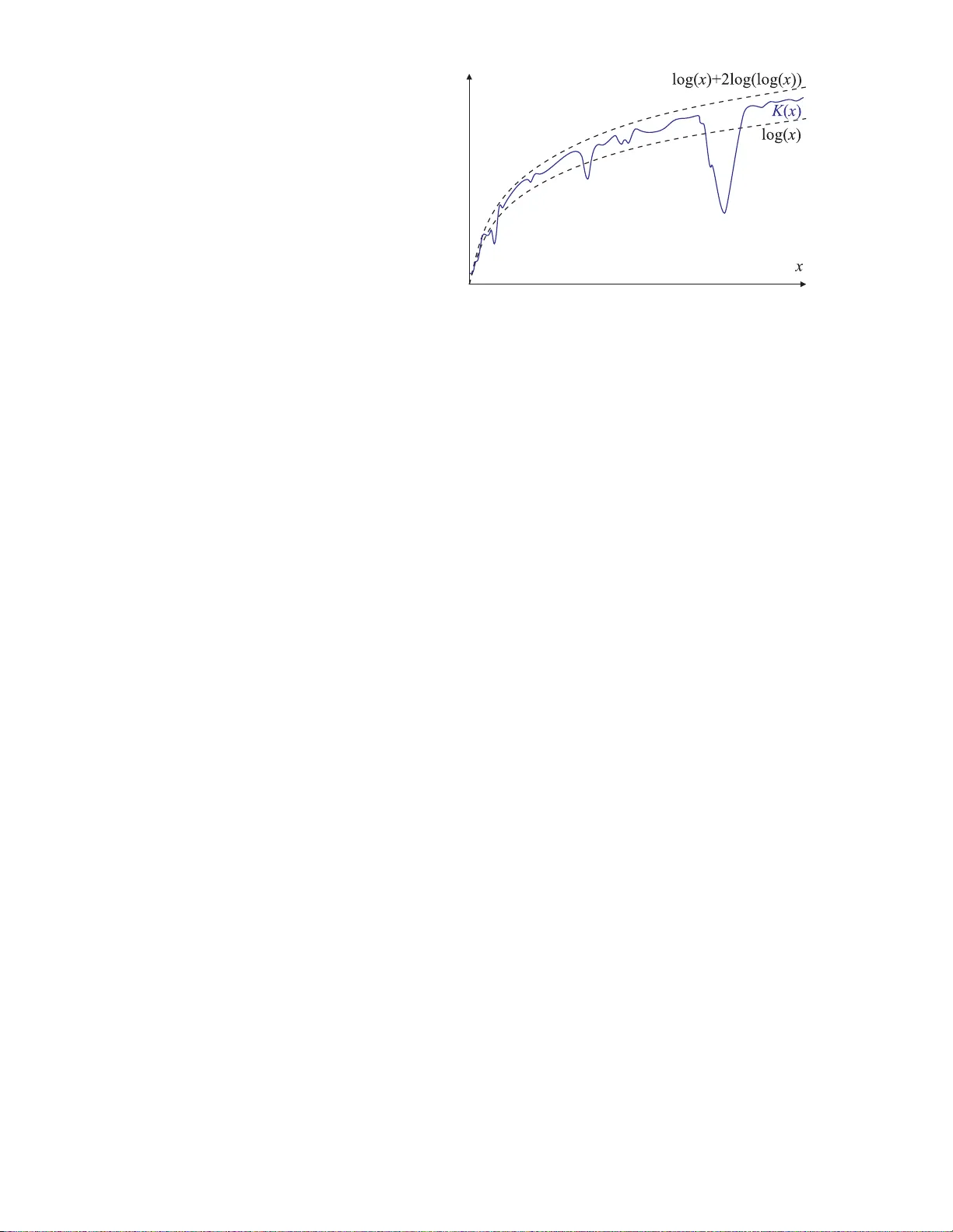
A Philosop h ical T reatise of Univ ersal Induction Sam uel Rathmanner and Marcus Hutter Researc h Sc ho ol of Computer Science Australian National Univ ersit y 25 Ma y 2011 Abstract Understanding ind u ctiv e r easoning is a pr oblem that has engaged mankind for thousands of y ears. This problem is relev an t to a wide r ange of ﬁelds and is in tegral to the philosophy of science. It h as b een tac kled by many great min d s ranging fr om ph ilosophers to scien tists to mathematicians, and more recen tly computer scient ists. In this article w e argue the case for Solomonoﬀ Ind uction, a f ormal in ductiv e framework wh ic h com b in es algorithmic information theory with the Ba y esian framework. Although it ac hiev es excellen t theoretical results and is b ased on solid philosophical foundations, the requisite tec hnical kno wl- edge necessary for understand ing this framewo rk h as caused it to remain largely unknown and un appreciated in the wider scien tiﬁc comm u nit y . Th e main con tri- bution of this article is to con vey Solomonoﬀ ind uction and its related concepts in a generally accessible form with the aim of b r idging this current tec hn ical gap. In the p ro cess we examine the ma jor historical contributions that hav e led to the formula tion of Solomonoﬀ In duction as w ell as criticisms of Solomonoﬀ and induction in general. In particular w e examine h o w S olomonoﬀ ind uction addresses many issu es that h a v e plagued other indu ctiv e sys tems, such as th e blac k rav ens p arado x and the conﬁ rmation p roblem, and compare th is appr oac h with other recen t approac hes. Keyw ords sequence prediction; inductiv e inference; Ba y es rule; Solomonoﬀ pr ior; Kol- mogoro v complexit y; Occam’s razor; ph ilosophical issu es; conﬁrmation theory; Blac k ra v en paradox. This article is de dic ate d to R ay Solomonoﬀ (1926–2 0 09), the disc over er and inventor of Universal Induction. 1 Con tents 1 In tro duction 3 1.1 Overview of Ar ticle . . . . . . . . . . . . . . . . . . . . . . . . . . . . . . . . . . . . . . 5 2 Broader Con text 6 2.1 Induction versus Deduction . . . . . . . . . . . . . . . . . . . . . . . . . . . . . . . . . 6 2.2 Prediction versus Induction . . . . . . . . . . . . . . . . . . . . . . . . . . . . . . . . . 7 2.3 Prediction, Concept Learning, Classiﬁca tion, Reg ression . . . . . . . . . . . . . . . . . 8 2.4 Prediction with Ex per t Advice versus Bay esian Lear ning . . . . . . . . . . . . . . . . . 9 2.5 No F ree Lunch versus Oc c am’s Razor . . . . . . . . . . . . . . . . . . . . . . . . . . . . 10 2.6 Non-Monotonic Reaso ning . . . . . . . . . . . . . . . . . . . . . . . . . . . . . . . . . . 11 2.7 Solomonoﬀ Induction . . . . . . . . . . . . . . . . . . . . . . . . . . . . . . . . . . . . . 11 3 Probabilit y 12 3.1 F requentist . . . . . . . . . . . . . . . . . . . . . . . . . . . . . . . . . . . . . . . . . . 12 3.2 Ob jectivist . . . . . . . . . . . . . . . . . . . . . . . . . . . . . . . . . . . . . . . . . . 13 3.3 Sub jectivist . . . . . . . . . . . . . . . . . . . . . . . . . . . . . . . . . . . . . . . . . . 14 4 Ba y es i anism for Prediction 16 4.1 Notation . . . . . . . . . . . . . . . . . . . . . . . . . . . . . . . . . . . . . . . . . . . . 18 4.2 Thomas Bay es . . . . . . . . . . . . . . . . . . . . . . . . . . . . . . . . . . . . . . . . 18 4.3 Mo dels, Hyp otheses and Environmen ts . . . . . . . . . . . . . . . . . . . . . . . . . . . 19 4.4 Bay es Theorem . . . . . . . . . . . . . . . . . . . . . . . . . . . . . . . . . . . . . . . . 21 4.5 Partial Hyp otheses . . . . . . . . . . . . . . . . . . . . . . . . . . . . . . . . . . . . . . 21 4.6 Sequence Predictio n . . . . . . . . . . . . . . . . . . . . . . . . . . . . . . . . . . . . . 22 4.7 Bay es Mixture . . . . . . . . . . . . . . . . . . . . . . . . . . . . . . . . . . . . . . . . 22 4.8 Exp ectation . . . . . . . . . . . . . . . . . . . . . . . . . . . . . . . . . . . . . . . . . . 23 4.9 Conv ergenc e Results . . . . . . . . . . . . . . . . . . . . . . . . . . . . . . . . . . . . . 24 4.10 Bayesian Decisions . . . . . . . . . . . . . . . . . . . . . . . . . . . . . . . . . . . . . . 26 4.11 Co ntin uo us Environment Classes . . . . . . . . . . . . . . . . . . . . . . . . . . . . . . 27 4.12 Cho o s ing the Mo del Cla ss . . . . . . . . . . . . . . . . . . . . . . . . . . . . . . . . . . 28 5 History 28 5.1 Epicurus . . . . . . . . . . . . . . . . . . . . . . . . . . . . . . . . . . . . . . . . . . . . 29 5.2 Sextus Empiricus a nd David Hume . . . . . . . . . . . . . . . . . . . . . . . . . . . . . 29 5.3 William of Ockham . . . . . . . . . . . . . . . . . . . . . . . . . . . . . . . . . . . . . . 31 5.4 Pierre- Simon Laplace and the Rule of Successio n . . . . . . . . . . . . . . . . . . . . . 32 5.5 Conﬁrmation Pro blem . . . . . . . . . . . . . . . . . . . . . . . . . . . . . . . . . . . . 34 5.6 Patric k Maher do es no t Capture the Logic of Co nﬁrmation . . . . . . . . . . . . . . . 37 5.7 Black Rav ens Paradox . . . . . . . . . . . . . . . . . . . . . . . . . . . . . . . . . . . . 39 5.8 Alan T uring . . . . . . . . . . . . . . . . . . . . . . . . . . . . . . . . . . . . . . . . . . 41 5.9 Andrey Kolmog orov . . . . . . . . . . . . . . . . . . . . . . . . . . . . . . . . . . . . . 42 6 Ho w to Cho os e the Prior 46 6.1 Sub jectiv e versus Ob jectiv e Prio rs . . . . . . . . . . . . . . . . . . . . . . . . . . . . . 47 6.2 Indiﬀerence Principle . . . . . . . . . . . . . . . . . . . . . . . . . . . . . . . . . . . . . 47 6.3 Reparametriza tion Inv ar iance . . . . . . . . . . . . . . . . . . . . . . . . . . . . . . . . 48 6.4 Regrouping Inv aria nce . . . . . . . . . . . . . . . . . . . . . . . . . . . . . . . . . . . . 49 6.5 Univ e r sal Prior . . . . . . . . . . . . . . . . . . . . . . . . . . . . . . . . . . . . . . . . 50 7 Solomono ﬀ Uni v ersal Prediction 51 7.1 Univ e r sal Bay es Mixture . . . . . . . . . . . . . . . . . . . . . . . . . . . . . . . . . . . 52 7.2 Deterministic Repres ent a tion . . . . . . . . . . . . . . . . . . . . . . . . . . . . . . . . 52 7.3 Old Evidence a nd New Hyp otheses . . . . . . . . . . . . . . . . . . . . . . . . . . . . . 55 7.4 Black Rav ens Paradox Using Solo mo noﬀ . . . . . . . . . . . . . . . . . . . . . . . . . . 56 8 Prediction Bounds 58 8.1 T otal Bounds . . . . . . . . . . . . . . . . . . . . . . . . . . . . . . . . . . . . . . . . . 58 8.2 Instantaneous Bounds . . . . . . . . . . . . . . . . . . . . . . . . . . . . . . . . . . . . 59 8.3 F uture Bounds . . . . . . . . . . . . . . . . . . . . . . . . . . . . . . . . . . . . . . . . 60 8.4 Univ e r sal is Better than Contin uous M . . . . . . . . . . . . . . . . . . . . . . . . . . 62 9 Appro ximations and Applications 63 9.1 Golden Standard . . . . . . . . . . . . . . . . . . . . . . . . . . . . . . . . . . . . . . . 63 9.2 Minim um Description Length Principle . . . . . . . . . . . . . . . . . . . . . . . . . . . 64 9.3 Resource Bounded Complexity and P rior . . . . . . . . . . . . . . . . . . . . . . . . . 65 9.4 Context T ree W eigh ting . . . . . . . . . . . . . . . . . . . . . . . . . . . . . . . . . . . 65 9.5 Univ e r sal Similarity Mea sure . . . . . . . . . . . . . . . . . . . . . . . . . . . . . . . . 66 9.6 Univ e r sal Artiﬁcial Intelligence . . . . . . . . . . . . . . . . . . . . . . . . . . . . . . . 66 10 Discussio n 67 10.1 P r ior K nowledge . . . . . . . . . . . . . . . . . . . . . . . . . . . . . . . . . . . . . . . 67 10.2 Dep endence on Universal T uring Machine U . . . . . . . . . . . . . . . . . . . . . . . . 68 10.3 Adv antages a nd Disadv antages . . . . . . . . . . . . . . . . . . . . . . . . . . . . . . . 68 10.4 Co nc lus ion . . . . . . . . . . . . . . . . . . . . . . . . . . . . . . . . . . . . . . . . . . 69 References 70 2 1 In tro duction According to Aristotle, it is o ur ability to reason whic h sets h umans a pa rt from the rest of the animal kingdom. The understanding a nd manipulation o f our en vironment tha t has made us so succes sful has only b een p ossible through this unique abilit y . Reasoning underpins ev ery h uman adv ancemen t and is used on a daily basis ev en if only trivially . Y et surprisingly , although reasoning is fundamen tal to the functioning and ev olution of our sp ecies, w e hav e had great diﬃcult y in pro ducing a satisfactory explanation of the mec hanism that go ve r ns a large p ortion of this reasoning; namely inductiv e reasoning. The diﬃcult y of any attempt at unrav eling the inner w orkings of the human mind should b e appreciated. Some hav e ev en argued that a complete understanding of the h uman mind is b ey ond the capabilities of the h uman mind [McG89]. Understanding ho w we reason is how eve r a n a r ea in whic h signiﬁcan t progress has b een made. Reasoning is of t en bro ken dow n into tw o bro ad catego ries. F ir stly there is de d uctive r e asonin g whic h can b e though t of as t he pro cess of dra wing logically v alid conclusions from some assumed or give n premise. Deductiv e reasoning is the type o f reasoning used in mathematical pro ofs or when dealing with formal systems. Alt ho ug h this t yp e of reasoning is o b viously necess ary it is no t alw ays adequate. When reasoning ab out our w orld we often w ant to mak e predictions that in v olve es- timations a nd generalizations. F or this w e use in d uctive r e a soning . Inductiv e reasoning can b e thought of as drawing the ‘b es t’ conclusions from a set of observ ations. Unfor- tunately these observ ations are almost alwa ys incomplete in some sense and therefore w e can nev er b e certain of the conclusions w e mak e. This pro ces s is analogous to the scien tiﬁc pro ces s in general. In science, rules and mo dels are found by generalizing patterns observ ed lo cally . These mo dels are then used to understand and predict our en vironmen t whic h in turn allows us to b eneﬁt, usually with great success. But like inductiv e inference, scien tiﬁc h yp otheses can nev er b e completely v alidated, so w e can nev er know whether they are true for certain. The diﬀerence b et wee n reasoning induc- tiv ely or deductiv ely can also b e simply though t of as the diﬀerence b etw een reasoning ab out the known or the unkno wn. Philosophically sp eaking t he fundamen tal goal of inductiv e reasoning is to gain a deep er a warenes s of ho w w e should maintain rational b eliefs and predictions in the face of uncertain ty and the unkno wn observ ations or problems of the future. In some sense a history of inductiv e reasoning is a history of questioning a nd attempting to understand our own though t pro cesses. As early as 300BC Epicurus w as intereste d in how w e judge comp eting theories for some giv en observ ations [Asm84]. This led him to p ostulate his pr inciple of multiple explanations whic h stated that w e should nev er disregard a consisten t t heory . William of Occam coun tered this with his with we ll- kno wn ‘Occam’s razor’ whic h advised that all but the simples t theory consisten t with the o bserv ations should b e discarded [Oc k90]. Hume lat er stated the problem of induction explicitly for the ﬁrst time “What is the founda tion of al l c onclusions fr om e xp erienc e ? ” [Hum39]. He also set a b out questioning the v a lidit y of suc h conclusions. Hume’s problem led Ba y es and Laplace to mak e the ﬁrst attempts a t formalizing inductiv e inference whic h has b ecome the basis f o r Ba ye sianism. This is a sc ho ol of though t that requires making 3 an explicit c hoice in the class of explanations considered and our prior b elief in eac h of them. Bay esianism has, in turn, fueled further attempts at formalizing induction. T o sa y that the history of induction has b ee n conten tious is an understatemen t [McG11]. There ha v e b ee n man y attempts a t formalizing inductiv e reasoning [GHW11] that address speciﬁc situations and satisfy many of the intuitiv e prop erties we expect of induction. Unfortunately most of these attempts ha ve serious ﬂaw s or are not g eneral enough. Man y of the results regarding induction ha ve b een con trov ersial and highly con tested, whic h is not particularly surprising. By its v ery nature induction deals with uncertain ty , sub j ectivity and c hallenging philosophical questions, and is therefore highly prone to discussion and debate. Ev en if a result is formally sound, its philo- sophical assumptions and applicabilit y in a range of situations are often questioned. In 1964 R ay Solomono ﬀ published the pap er “A F orm al The ory of I nductive I n- fer enc e” [Sol64]. In this pap e r he prop osed a univ ersal metho d of inductiv e inference whic h emplo ys the Ba y esian framew ork a nd his newly created theory of algorit hmic probabilit y . This metho d of Solomonoﬀ induction a pp ears to address the issues that plagued previous a ttempts at formalizing induction and ha s many promising prop erties and results. Solo mo no ﬀ induction and related concepts are the central fo cus of this article. The formalization of Solomonoﬀ induction mak es use of concepts and results from computer scienc e, statistics, information theory , and philosoph y . It is interesting that the dev elopmen t of a rigoro us formalization of induction, whic h is fundamen tal to almost all scien tiﬁc inquiry , is a highly m ulti-disciplinary undertaking, draw ing from these v arious a reas. Unfortunately this means that a high lev el of techn ical knowle dg e from these v arious disciplines is necess ary to fully understand the techn ical conte nt of Solomonoﬀ induction. This has restricted a deep understanding o f the concept to a fairly small prop ortion of academia whic h has hindered it s discussion and hence progress. In this article we attempt to bridge this ga p by conv eying the relev ant material in a muc h more a ccessib le form. In particular we hav e expanded the material in the dense 2007 pap er “On Universal Pr e dic tion and Bayesian Con ﬁ rmation ” [Hut07b] whic h arg ues that Solomonoﬀ induction essen tially solv es the induction problem. In addition to pro viding in t uitio n b eh ind the ov erall setup and the main results w e also examine the philosophical motiv at io ns and implications o f Solomonoﬀ ’s framew ork. W e ha v e a ttempted to write this article in such a wa y that the main prog ression of ideas can b e follow ed with minimal mathematical back g round. Ho we ver, in order to clearly comm unicate concrete results and to pro vide a more complete description to the capable reader, some tec hnical explanation is necessary . By making this know ledge mor e accessible w e hop e to promote discussion and a w a reness of these imp ortan t ideas within a m uch wider audience. E very ma jor con- tribution to the foundations of inductiv e reasoning has b een a con tr ibutio n to under- standing r ational tho ug h t. Occam explicitly stated our natural disp osition tow a rds simplicit y and elegance. Ba ye s inspired t he sc ho ol of Ba y esianism whic h has made us m uc h more a ware of the mec hanics b ehind o ur b elief system. No w, through Solomonoﬀ , it can b e argued that t he problem of formalizing o ptimal inductiv e inference is solv ed. 4 Being able to precisely fo rm ulate the pro cess o f (univ ersal) inductiv e inference is also h ugely signiﬁcan t for general artiﬁcial in telligence. Ob viously reasoning is synon ymous with intelligence , but true in telligence is a theory o f ho w to act on the conclusions w e mak e through reasoning. It may b e argued that optimal in telligence is nothing more tha n optimal inductiv e inference combined with optimal decision making. Since Solomonoﬀ provides optimal inductiv e inference and decision theory solve s the problem of c ho osing optimal actions, they can therefore b e com bined to pro duce in telligence. This is the approac h tak en by the second a ut ho r in deve loping the AIXI mo del which will b e discussed only brieﬂy . 1.1 Ov erview of A rticle Here w e will giv e a brief summary of t he con ten ts of this art icle. Se ction 2 lo oks at the broader context of (univ ersal) induction. A t ﬁrst we con- trast it with deduction. W e t hen argue that a n y inductiv e inference problem can b e considered or con v erted to a sequenc e prediction problem. This gives justiﬁcation for fo cusing on seque nce prediction throughout this article. W e also examine the relation b et we en Solomonoﬀ induction and o ther recen t appro a c hes to induction. In particular ho w Solomono ﬀ induction a ddresses non-monotonic r easoning and wh y it app ears to con tradict the conclusion of no-free-lunc h theorems. Se ction 3 cov ers probabilit y theory and the philosoph y b ehind the v arying sc ho ols of though t that exist. W e explain wh y the sub jectiv e inte rpreta t ion of probability is the most relev an t for univ ersal induction and wh y it is v alid. In particular w e explain wh y the b elief system of an y r ational agen t m ust ob ey the standard a xioms of probabilit y . Applying the axioms o f probability to mak e eﬀectiv e predictions r esults in the Ba y esian fra mework whic h is discusse d in depth in Se ction 4 . W e lo ok at what it means to b e a Bay esian; wh y mo dels, en vironmen ts and hy p othes es a ll express the same con- cept; and ﬁnally w e explain the mec hanics of the Bay esian f r amew ork. This includes lo oking at conv ergence results and how it can b e used t o make optimal Ba ye sian de- cisions. W e also lo o k brieﬂy at contin uous mo del classes and a t making reasonable c hoices fo r the mo del class. Se ction 5 g ives an o v erview of some of the ma jor historical contributions t o induc- tiv e reasoning. This includes the fundamen tal ideas of Epicurus’s principle of multiple explanations and Occam’s razor. W e also discuss brieﬂy the criticisms raised b y induc- tiv e sk eptics suc h as Empiricus and Hume. Laplace’s contribution is then examined. This includes the deriv ation of his famo us rule of succession whic h illustrat es ho w the Ba y esian framew ork can b e applied. This rule also illustrates the conﬁrmation problem that has pla g ued man y attempts at formalizing induction. The cause of this problem is examined and we sho w t hat a recen t claim by Maher [Mah04], that the conﬁrmation problem can b e solv ed using the axioms of probabilit y alone, is clearly unsatisfactory . One of the most diﬃcult problems with conﬁrmation theory is the black rav ens para do x. W e explain wh y this coun ter-in tuitive result arises and the desired solution. In order to understand the concept of K o lmogorov complexit y whic h is in tegral to So lo monoﬀ induction, it is necessary to brieﬂy examine the fundamental concept 5 of computabilit y and the closely related T uring mac hine. The in tro duc tio n of the theoretical T uring mac hine is in some w ay s considered the birth of computer science. W e lo ok at the ba sic idea of what a T uring mac hine is and ho w, through Solomonoﬀ, it b ecame an in tegral part o f univ ersal induction. The measure of complexit y that Kolmogorov dev elop ed is a ma jor part of algorithmic information theory . W e examine the in tuitio n b ehind it as w ell as some relev an t prop erties. In Se ction 6 we discuss reasonable approac hes to making a r a tional choice of prior as w ell as desirable prop erties for a prior to ha v e. The univ ersal prior inv o lv es the use of Kolmogorov complexit y whic h w e argue is highly intuitiv e and do es justice to b oth Occam and Epicurus. A t this p oint, ha ving in tro duced all the necessary concepts, Se ction 7 giv es an expla- nation of Solo monoﬀ ’s univ ersal predictor. W e examine tw o alt ernat e represen tations of this univ ersal predictor and the relat io nship b etw een them. W e also lo o k a t ho w this predictor deals with the problem of old evidence, the conﬁrmation problem and the blac k ra ve ns parado x. Se ction 8 discusses sev eral b o unds for this univers al predictor, whic h demonstrate that it p erforms excellen tly in general. In particular w e pr esen t tota l, instantaneous, and future erro r b ounds. Se ction 9 lo oks at the v alue o f Solomonoﬀ induction as a g old standard and how it ma y b e approx imated and applied in practice. W e men tion a n umber of approxim a tions and applications of either Solomonoﬀ or the closely related Kolmogo ro v complexit y . The extension of Solomonoﬀ to univ ersal artiﬁcial intelligenc e is also brieﬂy co v ered. Se ction 10 giv es a brief discussion of some of the issues concerning Solomonoﬀ induction as we ll as a review of the pro’s a nd con’s, and concludes. 2 Broader Con te xt The work done on the problem of induction, b oth philosophically and formally , has b een b oth v ast and v aried. In this article t he fo cus is on using inductiv e inference fo r making eﬀectiv e decisions. F rom this p ersp ectiv e, having an eﬀectiv e metho d of prediction is suﬃcien t. It is for this reason that this article fo cus es primarily on sequen ce prediction, rather than inference in t he narrow sense of learning a general mo del fro m sp eciﬁc data. Ev en concept learning, classiﬁcation, and regression problems can b e r ephrased as sequen ce prediction problems. After having clariﬁed these relat io nships, w e brieﬂy lo ok at Solomono ﬀ induction in the context o f some o f the most signiﬁcan t concepts in recen t discussions of inductiv e reasoning [GHW11] suc h a s Ba yes ian learning v ersus prediction with exp ert advice, no- free-lunc h theorems v ersus Occam’s razor, and non- monotonic reasoning. 2.1 Induction v ersus Deduction There ar e v arious inf o rmal deﬁnitions of inductiv e inference. It can b e though t of as the pro cess of deriving general conclusions from sp eciﬁc observ atio n instances. This is sort of dual to deductiv e inference , whic h can b e though t o f a s the pro cess of deducing 6 sp eciﬁc results fro m general axioms. These characterizations may b e a bit narrow and misleading, since induction and deduction a lso parallel each o ther in certain respects. The default system for deductiv e reasoning is “classical” (ﬁrst-order predicate) lo gic. The Hilb ert calculus starts with a handful of logical axiom sc hemes and only needs mo dus p onens as inference rule. T ogether with some domain- sp eciﬁc non- logical ax- ioms, this results in “theorems”. If some real- w orld situation (data , fa cts, o bserv ation) satisﬁes the conditions in a theorem, the theorem can b e applied to deriv e some con- clusions ab o ut the real w orld. The axioms in Z ermelo-F raenk el set theory are univ ersal in the sense tha t all of mathematics can b e formulated within it. Compare this to the (arguably) default system for inductiv e reasoning based on (real-v alued) probabilities: The Bay esian “calculus” starts with the Kolmogorov axioms of pro babilit y , a nd only needs Bay es rule for inference. Giv en some domain-sp eciﬁc prior and new data=facts=observ ations, this results in “p o sterior” degrees of b elief in v ario us h yp otheses ab out the world. Solomonoﬀ ’s prior is univ ersal in the sense that it can deal with arbitrary inductiv e inference problems. Hyp o t heses play the role of logical expressions, probability P ( X ) = 0 / 1 corresp onds to X b eing false/true, and 0 < P ( X ) < 1 to X b eing true in some mo dels but false in others. The general corresp ondence is depicted in the fo llowing table: Induction ⇔ Deduction T yp e of inference: generalization/prediction ⇔ specialization/deriv ation F ramew ork: probabilit y axioms b = logical axioms Assumptions: prior b = non-log ical a xioms Inference rule: Ba y es rule b = mo dus po nens Results: p osterior b = theorems Univ ersal sche me: Solomonoﬀ probability b = Zermelo-F raenk el set theory Univ ersal inf erence: univ ersal induction b = univ ersal theorem prov er 2.2 Prediction v ersus Ind uction The ab ov e c haracterization of inductiv e inference as the pro cess of going from sp eciﬁc to general w as somewhat narrow. Induction can also b e understo o d more broadly to include the pro cess of drawing conclusions a b out some giv en data, or ev en as the pro cess of predicting the future. Any inductive reasoning we do m ust b e based o n some data or evidence whic h can b e regarded as a history . F rom t his da t a we then make inferences, see patterns or rules or dra w conclusions ab out the gov erning pro cess. W e are not really inte rested in what this tells us ab out the already observ ed data since this is in the past and therefore static and inconsequen tial to future decisions. Rather w e care ab out what we are able to infer ab out future observ ations since this is what allo ws us to mak e b eneﬁcial decisions. In other w ords w e wan t to predict the natural con tinu a tion of our giv en history of observ ations. Note that ‘future observ atio ns’ can also refer to pa st but (so far) unkno wn historical ev ents that a re only rev ealed in the future. F rom this general p ersp ectiv e, the scien tiﬁc metho d can b e seen a s a sp eciﬁc case of inductiv e reasoning. In science w e make mo dels to explain some past data or obser- 7 v atio n history and these mo dels are then used to help us mak e accurate predictions. As humans we ﬁnd these mo de ls satisfying as w e like to hav e a clear understanding of what is happ ening, but mo dels are often o v erturned or revised in the future. Also, from a purely utilitarian p oin t of view, all that mat ters is our abilit y to mak e eﬀectiv e decisions and hence only the predictions and not the mo dels themselv es are of imp or- tance. T his is reminiscen t o f but not quite as strong a s the famous quote b y G eor g e Bo x tha t “Essen tially , all mo dels are wrong, but some are useful”. W e lo ok now at some sp eciﬁc examples o f ho w general induction problems can b e rephrased as prediction problems. 2.3 Prediction, Concept Learning, Classiﬁcation, Regression In many cases the form ulatio n is straight forw ar d. F or example, pro blems suc h as “what will the w eather b e lik e tomo r ro w?”, “what will the sto c k market do to morro w?” or “will the next rav en w e see be blac k?” are a lready in the form of prediction. In these cases all that needs to b e done is to explicitly pro vide an y relev an t historic data, suc h as sto c k mark et records or past w eather patterns, as a c hronological input sequence and then lo ok for the natural con tinuations of these sequence s. It should ho w ev er b e noted that a simple formulation do es no t imply a simple solution. F or example, t he c haotic nature of sto ck mark ets and w eather patterns mak e it extremely diﬃcult to ﬁnd the cor r ect contin uation of t his sequence, particularly mo r e than a few time steps ahead. More formally , in the ﬁeld of mac hine learning, sequence prediction is concerned with ﬁnding the con tinuation x n +1 ∈ X of an y giv en sequence x 1 , ..., x n . This may b e used to represen t a wide range of abstract problems b ey ond the obv ious application to time series data suc h as historical we a ther o r sto c k patterns. F or instance, (o n- line) concept learning, classiﬁcation and regression can b e regarded as sp ecial cases of sequence prediction. Concept learning inv o lv es categorizing ob jects into g roups whic h either do or don’t p ossess a giv en prop ert y . More formally , giv en a concept C ⊂ X , it requires learning a function f C suc h t ha t for all x : f C ( x ) = ( 1 if x ∈ C 0 if x / ∈ C Solomonoﬀ induction only deals with the problem of seque nce prediction; ho we ver, as w e discuss in the next pa ragraph, sequence prediction is general enough to also capture the problem of concept learning, whic h it self is a sp eciﬁc case of classiﬁcation. Although the setup a nd interpre ta tion of classiﬁcation using Solomonoﬀ may b e less in tuitive than using more traditional setups , the exce llent p erformance and generalit y of Solomo no ﬀ implies that theoretically it is unnecessary t o consider this problem separately . In machine learning, classiﬁcation is the problem of assigning some give n item x to its correct class based on its c har a cteristics and previously seen tra ining examples. In classiﬁcation w e ha ve data in the form of tuples containing a p oint and its asso ciated class ( x i , c i ). The go a l is to correctly classify some new item x n +1 b y ﬁnding c n +1 . 8 As b efore, all data is pro vided sequen tially with the new p oint x n +1 app ended at the end. In other w o rds, the classiﬁcation of x b ecomes “what is the next nu mber in the sequence x 1 c 1 x 2 c 2 ...x n c n x n +1 ?”. T ec hnically this could b e regarded as a sp eciﬁc case of regression with discrete function range, where the function w e are estimating maps the items to their resp ective classes. Regression is the problem of ﬁnding the f unction that is resp onsible fo r generating some giv en data p oin ts, often accounting for some noise or imprecision. The data is a set of (f eat ur e,v alue) tuples { ( x 1 , f ( x 1 )), ( x 2 , f ( x 2 )),....( x n , f ( x n )) } . In mac hine learning this problem is often ta c kled by constructing a function that is the ‘b es t’ estimate of the true function according t o the data seen so far. Alternativ ely , it can b e fo rmalized directly in terms of sequen tial prediction b y writing the input data as a sequence and app en ding it with a new p o int x n +1 for whic h w e wan t t o ﬁnd the functional v alue. In other words the problem b ecomes: “What is the next v alue in the sequence x 1 , f ( x 1 ) , x 2 , f ( x 2 ) , ...x n , f ( x n ) , x n +1 , ?”. Although this appro a c h do es not pro duce the function explicitly , it is essen tially equiv alen t, since f ( x ) for an y x can b e obtained by c ho osing x n +1 = x . 2.4 Prediction with Exp ert Ad vice v ersus Ba y esian Learning Prediction with exp ert advice is a mo dern approac h to prediction. In this setting it is assumed that there is some lar ge, p ossibly inﬁnite, class of ‘exp erts’ which mak e predictions ab o ut the giv en data. The aim is to observ e ho w eac h of t hese exp erts p erform a nd dev elop indep enden t predictions based o n this p erf o rmance. This is a general idea and may be carried out in v arious w ay s. Perhaps the simplest approach, kno wn as follow the leader, is to k eep t rac k of whic h exp ert has p erformed the b es t in the past and use its prediction. If a new exp ert tak es the lead, then your predictions will switc h to this new leading exp ert. Naiv ely the p erformance of an expert can b e measured b y simply counting the num b er of errors in its predictions but in man y situations it is appropriat e to use a loss function that weighs some errors as worse than o t hers. A v ariant o f this simple ‘follo w the leader’ concept is known as ‘follow the p e rt urb ed leader’ in which our predictions mimic t he leader most of the t ime but may switc h t o another with some sp eciﬁed probability [HP05]. This techniq ue giv es a proba bility distribution rather than a deterministic predictor which can b e adv antageous in man y con texts. The traditiona l Ba y esian framew or k discussed in this article uses a mixture mo del o ve r a h yp othesis or environmen t or mo del class, whic h resem bles the ‘follo w the p er- turb ed leader’ techniq ue. This mixture mo del reﬂects our rat ional b eliefs ab out the con tinu a tion of a seque nce giv en the p erformance of eac h “exp ert” and, as w e will see, p erforms very w ell theoretically . Solomonoﬀ induction uses the Bay esian fra mework with the inﬁnite class of “exp erts” giv en b y all computable env iro nmen ts. This means that there is alw ays an exp ert that p erforms w ell in an y giv en env ironment whic h allow s for go o d p erfo rmance without any problem-sp eciﬁc assumptions. 9 2.5 No F ree Lunc h v ersus Oc cam’s Razor This is in some w ay a con tra diction to the w ell-kno wn no-fr e e-lunch the or ems whic h state that, when a veraged ov er all p ossible data sets, all learning algorithms p erform equally well, and actually , equally p o orly [WM97]. There are sev eral v ariations of the no-free-lunc h theorem fo r par t icular contexts but they all rely on the assumption that for a general learner there is no underlying bias to exploit b ecause an y o bserv ations a r e equally p oss ible at an y p oint. In other w or ds, any arbitra rily complex en vironmen ts are just as lik ely as simple ones, or entirely ra ndom data sets are just as likely a s structured data. This assumption is misguided and seems absurd when applied to an y real w orld situations. If eve ry rav en w e hav e ev er seen has b een blac k, do es it really seem equally plausible that there is equal c hance that the next ra v en w e see will b e black , or white, or half blac k half white, or red etc. In life it is a necessit y to mak e general assumptions ab out the w orld a nd our observ a tion sequences and these assumptions generally perfo rm w ell in practice. T o ov ercome the damning conclusion of these no-fr e e-lunch the or em s in t he con- text of concept learning, Mitc hell introduced the follo wing inductiv e learning assump- tion whic h formalizes our in tuition and is esse ntially an implicit part of our reasoning [Mit90]. “A n y hyp othesis found to appr oximate the tar get function wel l over a suﬃciently lar ge set of tr aining examples wil l also appr ox i m ate the tar get function wel l over other unobserve d e xamples.” Similar assumptions can b e made for other contexts but this approach ha s b ee n criticized as it essen tially results in a circular line of reasoning. Essen t ia lly w e assume that inductiv e reasoning w orks b ecause it has w ork ed in the past but this reasoning is itself inductiv e and hence circular. Hu me’s arg umen t that this circularity in v alidates inductiv e reasoning is discussed further in Subsection 5 .2 . In fa ct this inductiv e learning assumption is closely related to what Hume called the principle of uniformit y of na t ur e. A principle he said w e implicitly , but in v alidly , assume. If we prescribe Occam’s r a zor principle [Oc k90 ] to select the simplest theory con- sisten t with the training examples and assume some general bias tow ards structured en vironmen ts, one can prov e tha t inductiv e learning “works ” . These assumptions are an in tegral part of our scien tiﬁc metho d. Whether they admit it or not, ev ery scien tist, and in fact eve ry p erson, is con tin uously using this implicit bias to w a r ds simplicit y and structure to some degree. An y agen t, animal or ma chine, mus t mak e use of underlying structure in some form in order to learn. Although induction inheren tly inv olves dealing with an uncertain en vironmen t for which no hard guarantee s can b e made, it is clear that our world is massiv ely structured and that exploiting structure in general is the b e st tec hnique for p erforming we ll. By deny ing the relev ance of this structure no-fr e e-lunch the or ems imply that general learning, and the concept of g eneral in telligence, is essen tially futile, whic h con t r a dicts o ur exp erience. Solomonoﬀ induction is witness to the p ossibilit y of general learning, a ssuming only some structure in the env iro nmen t without having to sp ecify whic h t yp e of structure, and using Occam’s razor. 10 2.6 Non-Monotonic Reasoning Non-monotonic reasoning is a nother concept that has b een discusse d recen tly in relatio n to induction. This concept attempts t o solv e t he problem o f formalizing common sense log ic. When a rtiﬁcial in telligence researc hers a ttempted to capture ev eryday statemen ts o f inference using classical lo gic they b egan to realize this w as a diﬃcult if not imp ossible task. The problem a r ises largely b e cause of the implicit assumption of normalit y w e often mak e to exclude exceptional circumstances . F or example, it w ould b e p erfectly acceptable to mak e a statemen t suc h as “the car star t s when you turn the k ey in the ignition” [G HW11]. Therefore if w e let F ( x ) b e the predicate that we turn the k ey in the ignition in car x, and S ( x ) b e the predicate that x starts, then the previous sen tence w ould b e represen ted b y the logical statemen t F ( x ) ⇒ S ( x ). Of course there are man y reasons why this might not b e correct suc h as t he fact that the car x has no fuel or a mec hanical problem. But these exceptions do not stop us making these types of statemen ts b ecause it is implicit y assumed t hat this statemen t may only hold under normal conditions. This assumption of normal conditions also leads to a lo gic that is non- monotonic in its argumen ts. Normally if the statemen t A ⇒ C ho lds, then it follow s logically that A ∧ B ⇒ C . How ev er this rule may no longer hold using ‘normal case’ reasoning. If G ( x ) is the predicate that x ha s no fuel then, although the statemen t F ( x ) ⇒ S ( x ) is (normally) true, F ( x ) ∧ G ( x ) ⇒ S ( x ) is (normally) not t r ue, since the car will not start without fuel. Another example is that a general rule in our kno wledge ba se may b e that “birds can ﬂy”. Therefore if x is a bird it is natural t o assume tha t x can ﬂy; ho w eve r if x is a bird and x is a p enguin then it is no lo nger correct to sa y that x can ﬂy . 2.7 Solomonoﬀ Indu ction Solomonoﬀ induction [Sol64] b ypasses this issue entirely b y av oiding the use of strict logical syn tax which seems to b e an inadequate to ol for dealing with any reasonably complex or real-world en vironmen t. Non-monotonic statemen ts suc h as the examples sho wn can b e programmed in a v ariet y of wa ys to eﬀectiv ely deal with ‘the normal case’ and an arbitrary num b er of exceptional cases. This means that there exists a com- putable en vironmen t in Solomonoﬀ ’s univ ersal class whic h will eﬀectiv ely describe the problem. The non- monotonicit y of the en vironmen t will certainly aﬀect its complexit y and hence its prior but a simple non- mo no tonic en vironmen t will still hav e a reasonably high prior since there will b e a reasonably short wa y of expressing it. More generally the complexit y , and hence prio r (see Subsection 6.5), of a non- monotonic environme nt will dep end on t he v ariet y and n um b er of exceptions to the general rules, but this seems to b e a desirable prop erty to ha ve . The implicit assumption o f normality we use is due to our prior exp erience and kno wledge of the real w orld. Initially , for an ag en t acting in an unkno wn en vironment, it seems reasonable tha t up on b eing told a general rule, it should assume the rule to hold in all cases and then learn the exceptional cases as t hey a r e observ ed or inferred. This is essen tially ho w Solomonoﬀ induction b eha ve s. Because of the fundamental w ay in whic h Solomonoﬀ ’s univ ersal induction sc heme 11 con tinu o usly lear ns and improv es fr o m its exp erience, it ma y b e arg ued that a ny useful computable approach to induction in one wa y or another a ppro ximates Solomonoﬀ induction. In any case it app ears to compare w ell with the ab ov e approac hes. The ma jor issue remains its incomputabilit y and the diﬃculty o f appro ximating Solomonoﬀ in reasonably complex en vironmen ts. This is discussed furt her in Section 9. 3 Probabilit y In order to fully appreciate the Bay esian framew ork it is imp ortant to hav e some understanding of the theory o f probability that it is based on. Probability theory has had a long and con tentious history [Go o83 , Jay03, McG11]. Ev en to da y probability theory divides the scien tiﬁc comm unity with sev eral comp eting sc ho ols of though t whic h stem lar gely f rom the diﬀerent metho ds of dealing with uncertain ty as it app ears in diﬀeren t a r eas of scienc e. The most p o pular of these are ob jectiv e, sub j ective and frequen tist whic h reﬂect fundamen tally diﬀeren t philosophical in t erpretatio ns of what probabilit y means. Surprisingly it turns out that these in terpretations lead to the same set of axioms and t herefore these philosophical diﬀerences a r e of little imp ortance in practical applications. It is ho wev er w ort h considering these diﬀerences when lo oking at our motiv ation in t he con text o f induction. In the follow ing Ω is used to denote the sample space whic h is the set of a ll p ossible outcomes. An even t E ⊂ Ω is said to o ccur if the outcome is in E . F or instance when thro wing a die t he sample space Ω is { 1 , 2 , 3 , 4 , 5 , 6 } and an ev en t E is some sp ec iﬁc subset of these o utcomes. F or instance, the ev en n umbers is the ev ent E = { 2 , 4 , 6 } and the set o f n um b ers less than 3 is the ev en t E = { 1 , 2 } . 3.1 F requen tist The frequen tist approach is the most in tuitiv e in terpretation of probabilities, ho w eve r it has sev eral crippling dra wback s and is not a pplicable in man y situatio ns where we w ould lik e it to b e. A frequen tist deﬁnes the pr o babilit y of an ev en t as the limiting frequency of this ev ent relative to the en tire sample space Ω. F ormally if k ( n ) is the n um b er of t imes that ev en t E o ccurs in n trials then P ( E ) := lim n →∞ [ k ( n ) /n ]. F or example when throw ing a die the probability of throwing a 6 is deﬁned as the ratio o f the n umber of thro ws tha t come up 6 to the n um b e r of throws in total as the num b er of throws go es to inﬁnity . Aft er man y t hro ws we exp ect this nu mber to b e close to 1 / 6 . Th is is often one of the wa ys the concept of probabilit y is taught, whic h is part of the reason that it app eals to our in tuition. Ho wev er when examined more closely it b ecomes apparent t ha t this deﬁnition is problematic. No matter how large n gets there is no gua r a n tee that k ( n ) /n will conv erge to P ( E ). Ev en if the die is thrown a million times it is conceiv able although extremely unlik ely that ev ery roll will pro duce a 6 o r that half the r o lls will pro duc e a 6 . The b est w e can sa y is that as n increases, the probability that k ( n ) / n is arbitrarily close to P ( E ) also increases and will ev en tually get arbitrarily close to 1. F ormally this is 12 stated as k ( n ) / n con ve rg es to P ( E ) with probability 1. Unfortunately t his give s rise to a circularity as the concept of probabilit y is then used in deﬁning probabilit y . Another problem with the frequen tist appro ac h is that there ar e man y situations where it is not applicable. Consider the b etting o dds in a horse race. If the o dds on a horse are, for instance, 3 : 1 this is equiv alent to sa ying that the pro babilit y that the horse will win is 0 . 25. This is certainly not the same as sa ying that the ho rse has w on 1 in ev ery 4 previous r a ces. Instead it represen ts the b o okies b elief that the horse will win whic h dep ends on many factors. This pro babilit y as b elief in terpretation is the basis of the sub jectivist’s understanding. The error here may app ear to b e in asso ciating pr o babilities with b etting o dds and it could b e arg ued that strictly sp eaking the probability of the horse winning should b e deﬁned a s the ratio o f wins t o o v erall races in the past, but this idea quic kly b ecomes inconsisten t. Clearly it mak es no sense to equally w eigh ev ery race the horse has b een in to ﬁnd the probability o f the horse winning this particular race. The races might therefore b e restricted to tho se held on the same track and against the same horses, but since the we a t her and age o f the horse might also b e a f actor there w o uld b e no other races with whic h to compar e. This c ho ice of reference class p oses a very real problem in some practical situations suc h as medical diagnosis [Rei49]. The frequency approac h is only really applicable in situations where w e can draw a la rge n umber of samples from a distribution that is indep enden t and iden tically distributed (i.i.d.) such as ﬂipping a coin. 3.2 Ob jectivist The ob jectivist in t erpretatio n is that probabilities are real prop erties of ob jects a nd of the world and therefore the ob jectivist b eliev es that the w orld a ctually inv olv es inheren tly random pro cesses. This p oin t of view has b een largely supp orted by the success o f quan tum phy sics whic h states tha t there is tr ue randomness presen t at a sub-atomic leve l. The most widely accepted set of axioms fo r ob jectiv e probabilities are due to Ko lmogorov [Kol33] and are giv en here. Kolmogoro v’s P r obabilit y axioms. • If A a nd B are ev ents, then the intersec tio n A ∩ B , the unio n A ∪ B , and the diﬀerence A \ B are also ev ents. • The sample space Ω and the empt y set {} are ev en ts. • There is a function P that assigns non negative real num b ers, called pr o babilities, to eac h ev en t. • P (Ω) = 1 and P ( {} ) = 0 . • P ( A ∪ B ) = P ( A ) + P ( B ) − P ( A ∩ B ) • F or a decreasing sequence A 1 ⊃ A 2 ⊃ A 3 ... of ev en ts with ∩ n A n = {} w e ha v e lim n →∞ P ( A n ) = 0 In addition to the axioms there is the imp ortant deﬁnition of conditio nal probabilit y . If A and B are ev en ts with P ( A ) > 0 t hen the probability that ev en t B will o ccur 13 under the condition that ev en t A o c curred is P ( B | A ) = P ( A ∩ B ) P ( A ) One of the problems with these axioms is that they only uniquely determine v alues for the n ull ev en t and the ev en t of the en tire probabilit y space. Although there are general principles for assigning v alues to o ther ev ents, ﬁnding a univ ersal formal metho d has b een problematic. Applying general principles often requires some degree of sub jectiv- it y which can lead to debate. Kolmogor ov complexit y which is examined la t er prov ides a promising univers a l framew ork. It has b een argued [Hut05, Sc h97 ] that the ob jectiv e interpre ta tion places to o m uch faith in the ultimate tr uth of the quantum phy sics mo del. A simple example of ra n- domness b ein g incorrectly attributed to a pro ces s is the ﬂipping of a coin. This is the standard a nalogy used in almost an y situation where tw o outcomes o ccur with pro b- abilit y 0 . 5 each, with heads and tails represen ting t he resp ectiv e outcomes. T his is b ecause when w e ﬂip a coin the proba bility of heads is, for all practical purp oses, 0 . 5. Ev en in this article w e used this example to represen t a truly sto c hastic pro cess, but in realit y the probability of heads is actually (close to) 1 or 0 the momen t the coin leav es y our ﬁnger. This is b ecause the pro cess is not inheren tly random a nd if the exact ini- tial conditions a re kno wn then the o utcome can b e calculated b y applying the laws of ph ysics. This statemen t is somewhat questionable as w e ma y debate that an unknow n breeze ma y aﬀ ect the outcome o r that our calculations w ould also need t o consider the exact p oint that the coin lands whic h, if it w as caught, w ould dep end o n the p erson. These ob jections are mute if w e consider exact kno wledge of initial conditions to in- clude all lo cal weather conditions and the p ers ons state of mind. Without going into the question of free will the p oin t is simply that w e often use randomness to a ccoun t for uncertain t y in a mo del or a lack of adequate kno wledge. P erhaps quan tum ph ysics is analogous to this in that although the mo del is curren tly very successful, there may b e a time when the ‘inheren t’ r a ndomness can b e deterministically accoun ted for b y a more accurate mo del. In cases where the data is i.i.d., t he ob jectiv e probability is still iden tiﬁed with the limiting frequency , whic h is wh y these inte rpr eta t io ns coincide for these cases. It is also p ossible to deriv e these axioms from the limiting frequency deﬁnition, how ev er b y using these axioms as a starting p oint the issues encoun tered b y the fr equen tist ar e a voide d. 3.3 Sub jectivist It is the sub jectivist interpretation of probability that is most relev ant in the contex t of induction, particularity in relation to agen t based learning. The sub jectivist interprets a pro ba bilit y of an ev en t as a degree of b elief in the eve nt o ccurring and when any agen t , h uman included, is attempting to learn ab out its en vironmen t a nd act optimally it is exactly this degree of b elief that is imp ortan t. If a probability deﬁnes a degree of b elief it must b e sub j ective and therefore ma y diﬀer from agen t to agent. This ma y seem unscien tiﬁc or unsatisfactory but when 14 examined philosophically this in terpretation ha s a strong case. T o see this, consider Scott a nd F red gambling in Las V egas. While playing roulette they observ e tha t the ball la nds on 0 an abnormally high n umber of t imes causing them to lose signiﬁcan tly . Giv en that they are in a large we ll- kno wn Casino, F red thinks nothing o f t his abnor- malit y b elieving tha t they hav e probably just b een v ery unlucky . Scott on the other hand kno ws some of the employ ees a t this particular Casino and has heard rumors of corruption on the roulette tables. This extra information can b e thought o f as ob- serv ations that when com bined with the statistical abnormality of the roulette table raises Scott’s b elief that they ha ve b een victim to foul play . It is inevitable t ha t, con- sciously or not, our analysis a nd interpretation of an y situation will b e biased b y our o wn b elie fs, exp erience a nd kno wledge. In a ve ry formal sense this means that our probabilities are a function of our en tire previous p ersonal history and this is exactly ho w Solomono ﬀ ’s prediction sc heme can b e used. As a simple example consider F red and Scott eac h indep endently dra wing balls from an ur n, with replacemen t, which contains black and white balls in an unkno wn ratio. Imag ine that F red draw s 50 white balls and 20 blac k balls while Scott dra ws 30 white balls and 4 0 blac k balls. This is p o ssible for an y true ratio as long as there is a p ositive fraction of b oth black and white. Clearly F red will b eliev e that the ra tio of white to blac k is appro ximately 5 : 2 while Scott will b eliev e that it is appro ximately 3 : 4. The p oin t is that b oth of these b eliefs are completely v alid giv en their respective observ ations regardless of the true ratio. Although w e may accept that proba bilities a re sub jectiv e it is vital that there is a formal system that sp eciﬁes ho w to up da te and manipulate these b elie f v alues. It is here that the sub jec tive interpretation of pro babilit y has faced many criticisms as it w as arg ued that sub jective b elief v alues don’t ob ey f o rmal mathematical rules or that the rules they do ob ey are also sub jectiv e making formalization diﬃcult or imp oss ible. It is a surprising and ma jor result tha t any rational ag en t must up date its b eliefs b y a unique system whic h coincides with that of limiting frequencies and ob jectiv e probabilities. The most in tuitive justiﬁcation for this is fro m a D ut ch b oo k argumen t whic h sho ws that if an ag en t’s b eliefs are inconsisten t (contradict the axioms) then a set of b ets can b e fo r mulated whic h the ag ent ﬁnds fav ora ble a ccording to its b eliefs but whic h guaran tees that it will lose. The Dutch b o ok argumen t is how ev er not rigorous and there are sev eral o b jections to it [Ear93]. T he main issue rests o n t he implicit assumption that b elief states uniquely deﬁne b etting b ehav ior whic h has b een called in to ques t io n since there are other psyc hological factors whic h can hav e an aﬀect. F or example in a game of p ok er it is often rational for a pla yer to b et an amount tha t do es not reﬂect his b elief in winning the ha nd precisely b ecause he is trying to bluﬀ or con v ey a w eak hand [Sch 8 6 ]. In 1946 Co x published a theorem t ha t ga ve a fo rmal rigorous justiﬁcation that “if de gr e es of plausibi l i ty ar e r e p r ese nte d b y r e al numb e rs , then ther e is a uniq uely determine d set o f quantitative rules for c onducting infer enc e” [Ja y03] and that this set of rules is the same as those giv en b y the standard probabilit y axioms. Co x’s axioms for b elief s. 15 • The degree of b elief in an ev ent B , g iv en that ev en t A has o ccurred can b e c haracterized b y a real- v alued function B el ( B | A ). • B el (Ω \ B | A ) is a t wice diﬀerentiable function of B el ( B | A ) for A 6 = {} . • B el ( B ∩ C | A ) is a twic e diﬀeren tiable function of B el ( C | B ∩ A ) and B el ( B | A ) for B ∩ A 6 = {} . This uniﬁcation and veriﬁcation of the probabilit y axioms is a signiﬁcan t result whic h allo ws us to view the frequen tist deﬁnition as a sp ecial case of the sub jectiv ist in ter- pretation. This means t hat the in tuitive ly satisfying asp ect o f the frequen tist in terpre- tation is not lost but no w obtains a new ﬂav or. Consider again the case of determining the ra tio of blac k to white balls in an urn through rep eated sampling with replacemen t where the true ratio is 1 : 1. As the urn is rep eatedly sampled the relative fr equency and hence sub jectiv e b elief that the next ball is white will con v erge with proba bility 1 to 0 . 5. Altho ugh this is the correct probability it is imp ortan t to realize that it is still a belief and not an inheren t prop erty . In the unlik ely but p ossible ev en t that a white ball is sampled 1000 times the sub jective probability /b elie f tha t the next ball will b e white w o uld b e v ery close to 1. This understanding of probability can b e troubling as it sugg ests that w e can nev er b e certain of any truth ab o ut reality , ho we ver this corresp onds exactly with the phi- losoph y of science. In science it is not p ossible to ev er prov e a hy p othesis , it is only p ossible to dispro ve it. No matter how muc h evidence there is for a h yp o thesis it will nev er b e enough to mak e its truth certain. What are often stated a s phys ical la ws are actually o nly strongly b eliev ed and heav ily tested hypotheses. Science is not imp eded b y this fact how eve r. On the con trary , it allow s for constan t questioning and progress in the ﬁeld and, alt ho ugh mo dels may neve r b e completely prov en, it do es not stop them b eing usefully applied. 4 Ba y esianism for Pre diction T o fully appreciate the historical at t empts to solve the problem o f induction and the corresp onding discus sions whic h fueled t he ﬁeld it is neces sary to ﬁrst understand the Ba y esian framew ork. But b efore explaining the mec hanics of the Bay esian framew ork it is w orth ha ving a brief lo ok at what it means to b e a Bay esian. G iving a precise ex- planation is diﬃcult due to the v ario us in terpretations of Ba ye sianism [Go o71, Go o83], ho w eve r all Bay esians share some core concepts. Being a Bay esian is of ten simply asso ciated with using Bay es form ula but this is a gross simpliﬁcation. Although Ba y es f o rm ula pla ys an imp or t a n t role in the Ba ye sian framew ork it is not unique to Bay esians. The rule is directly deriv ed from the axioms o f probabilit y and therefore its correctness is no more debatable than that of the axioms of probability . More imp o r tan t to Bay esianism is Cox’s result that a ra t ional b elief system m ust ob ey the standard probability axioms. This is b ecause a Bay esian is a sub jectivist, b elieving that our b elie fs and hence probabilities a re a result of our p ersonal history . In other w or ks, what w e b eliev e to day dep ends on what w e b eliev ed y esterda y and 16 an ything w e hav e learnt since y esterda y . W hat w e b eliev ed yes terday dep ends on what w e b eliev ed the day b efore, and so forth. Tw o individuals with v ery diﬀerent histories may therefore hold diﬀeren t b eliefs a b out the same ev ent. This means that the pro ba bilit y of the ev en t for eac h individual can b e v alidly diﬀeren t from eac h other as long as t hey bo th up dated their b eliefs in a rationally consisten t manner. This rational up dating pro cess is at the core of Bay esianism. It ma y seem unsci- en tiﬁc t ha t diﬀeren t individuals can assign distinct y et v a lid probabilities but, as we ha v e seen in Subsection 3.3, this can b e quite reasonable. There is a strong link to the frequen tist approach here. If the t wo individuals a r e giv en the same observ atio ns, or at least observ ations from the same source, then their beliefs should ev en tually conv erge b ecause their f r equen tist estimate should con v erge. Philosophically sp eaking, how eve r, diﬀeren t individuals will nev er observ e precisely the same observ ations. Each hum a n has a unique exp erience of the world around them and therefore their b eliefs will neve r b e iden tical. A Bay esian’s b elief ab out ev ents is g ov erned b y b eliefs in the p ossib le causes of those eve nts. Ev erything we see has many p ossible explanations although we may only consider a f ew of them t o b e plausible. T o b e able t o up da te b eliefs consisten tly a Ba y esian m ust ﬁrst decide on the set of all explanations that ma y b e p ossible. When considering a sp eciﬁc exp erimen t this set o f explanations, or h yp otheses, need only explain t he o bserv ations p erta ining to the exp erimen t. F or example when ﬂipping a coin to ﬁnd its bias, t he h yp otheses may simply b e all p o ssible biases of the coin. F or univ ersal induction, w e are interes ted in ﬁnding the true go ve rning pro cess b ehind our en tire reality and t o do this we consider all p oss ible w orlds in a certain sense. No matter what the problem is we can alw ay s consider it to consist of an agent in some unkno wn en vironmen t. In the coin example all irrelev ant information is discarded and the environme nt simply consists o f observing coin ﬂips. It is useful to k eep this general setup in mind throughout this article. Lastly , the agent m ust hav e some prio r b elie f in these explanations b efore the up dating pro cess b egins. In other words b efore any observ ations ha ve b een made. Our b eliefs to da y dep en d on b e liefs y esterda y whic h dep end on the day b efore. But at some p oin t there is no ‘da y b efo re’ whic h is why some initial b elief is required to b egin the pro cess. O v er a lo ng enough p erio d these initia l b eliefs will b e ‘wash ed out’ but realistically they are imp o rtan t and should b e c hosen sensibly . Summing up, a Ba y esian holds b eliefs ab out an y p o ssible cause of an ev en t. These b eliefs dep end on all previously obtained informat ion and are therefore sub jectiv e. A b elief system that is en tirely consisten t with the Bay esian framew ork is ob viously unrealistic as a mo del for h uman reasoning a s this w o uld require p erfect lo g ical up dating at ev ery instance as w e con t inuously receiv e new informatio n. There are also emotional and psyc holo gical f a ctors that come in to play for h umans. Ra ther this is an idealized goal, or g old standard, which a Ba y esian thinks w e should striv e f or if w e are to b e completely ra t io nal. 17 4.1 Notation In order to examine some of the more tec hnical con tent and results it is necessary to ﬁrst establish some notation. Throughout the article X will represen t the alphab et of the observ ation space b eing considered. This is simply the set o f characters used to enco de the observ ations in a particular situation. F or example when ﬂipping a coin and observing heads or tails, X = { H ead, T ail } or { h, t } or { 1 , 0 } . An o bserv ation sequence is enco ded as a string ov er the alphab et whic h is usually denoted x . In some cases we are intereste d in the length of x or some subsection of x . x 1: n denotes a string of length n or, dep ending on con text, the ﬁrst n bits of x . x m denotes t he m th bit of x . x 0 from now on. An imp ortan t mathematical prop erty of this mixture mo del is its dominance. ξ ( x ) ≥ w ν · ν ( x ) ∀ x and ∀ ν ∈ M , in particular ξ ( x ) ≥ w µ · µ ( x ) This means that t he proba bility of a particular observ ation under Ba ye s mixture is at least as great as its probabilit y under any particular h yp ot hesis in pro p ortion to the prior b elief in that hypothesis. This is t r ivial to see since the proba bilit y under Ba y es mix is simply obta ined b y summing the probabilities under eac h hypothesis prop ortional to its prior a nd these are all non-negative . In particular this result applies to the true distribution µ . This prop erty is crucial in pro ving the follo wing conv ergence results. 4.8 Exp ectation Since our predications deal with p ossibly sto c hastic en vironmen ts, exp ectation is an imp ortant concept in examining p erforma nce. When there is random c hance in v olv ed in what rew ards ar e gained, it is diﬃcult to make guara ntees ab out the eﬀect of a single action. The action that receiv es a higher rew a rd in this instance ma y not b e 23 optimal in the long run. As lo ng as we hav e arbitrarily many tries, the b est strategy is to c ho ose the action that maximizes the exp ected rew ard. This is particularly relev an t in relation to agen t based lear ning , In general, exp ectation is deﬁned for some function f : X n → R , whic h assigns a real v alue to an observ a tion sequ ence of any length in the following wa y: E [ f ] = X x 1: n ∈X n µ ( x 1: n ) f ( x 1: n ) This can b e thought of as the av erag e v alue o f a function under the true distribution. When we talk a b out maximizing an agent’s expected rew ard t he function b eing con- sidered is the agent’s utilit y function and this is generally the most imp orta n t v alue. F or example, when give n the c hoice b etw een a certain $10 or a 50% c ha nce a t $100 the rational c hoice is to take the latter option as it maximizes one’s expectation, assuming monetary v alue deﬁnes utilit y . Exp ectation is an essen tial concept for making go od decisions in any sto c hastic en vironmen t. In p o k er, fo r example, a go o d play er uses exp ectation con tinuous ly , althoug h the calculations ma y even tually b ecome instinctual to a large degree. In general a play er’s decision to contin ue in a hand dep ends on whether the exp ected return is larg er than the a mo unt the pla yer mus t in v est in the hand. In the case of T exas hold’em p o k er the true en vironmen t is the distribution giv en b y the shu ﬄed dec k and the function is the exp ected return on some sequence o f communal cards. It should also b e noted that this is not a stationa r y en vironmen t: the distribution changes conditioned on the new information av ailable in the comm unal cards. 4.9 Con v ergence Results F or the Ba ye sian mixture to b e useful it is imp ortant that it p erforms well. As the accuracy of predictions is the primar y concern, the p erfo r ma nce of a distribution is measured by how close its predictions are to those of the true env iro nmen t distribution. The ana lysis of this p erformance v aries dep ending on whether the true en vironmen t is deterministic or sto c hastic. Deterministic. In the deterministic setting the accuracy is easier to determine: As an observ ation either will or won’t b e observ ed, there is no uncertain ty . F or a deterministic en vironmen t it is suﬃcien t to kno w the unique observ atio n sequence α that m ust b e generated, since it contains a ll the info rmation of the en vironmen t. F ormally µ ( α 1: n ) = 1 for all n where α 1: n is the initial n elemen ts o f α , a nd µ ( x ) = 0 f or a n y x t ha t is not a preﬁx of α , i.e. there is no n suc h t ha t x = α 1: n . In this deterministic case the follo wing results hold ∞ X t =1 | 1 − ξ ( α t | α 0 and a- p osteriori asymptotically all mass P ( θ p | 1 n ) → 1. Instead of θ = 1 it is also p ossible to form ula t e the hypothesis “all ra v ens a re blac k” as the observ at io n sequence of an inﬁnite n umber of black rav ens, i.e. H ′ = x = 1 ∞ where a 1 is a black rav en. This purely observ a t io nal in terpretation might b e considered philosophically more appropria te since it considers only observ able data rather than an unobserv able para meter. Ho we ver the same problem o ccurs. If x 1: n = 1 n is a sequence of n black ra v ens, then P ( x 1: n ) = n ! / ( n + 1)! = 1 / n +1 . Therefore P (1 k | 1 n ) = P (1 n + k ) P (1 n ) = n n + k This means that for an y ﬁnite k our b elief in the h yp othesis that w e will observ e k more blac k rav ens conv erges to 1 as the num b er of observ ed rav ens n tends to inﬁnity , whic h is not surprising and conforms to intuition. Once w e ha ve seen 10 0 0 blac k ra ve ns w e strongly exp ect that we will observ e ano ther 10 bla ck ra ve ns. How ev er for the ab ov e h yp othesis of “a ll rav ens are blac k” k is inﬁnite and the probabilit y P (1 k = ∞ | 1 n ) will b e zero for any num b er n of observ ed rav ens. By making the reasonable assumption that the p opulation o f rav ens is ﬁnite, and therefore that k is ﬁnite, we may exp ect to ﬁx the problem. This is the approac h tak en b y Maher [Mah04]. Ho w ev er it still leads to unacceptable results whic h w e examine further in the next subsection. Since b oth forms of the unive r sal generalization fail to b e conﬁrmed b y the rule of success ion, there seem to b e only t w o reasonable options. W e can simply accept that h yp otheses corresp onding to exact v alues of θ can not b e conﬁrmed, so instead soft h yp otheses corresp o nding to small in terv als or neigh b orho ods must b e used. While we can successfully r eason ab out soft hypotheses, w e still ha v e to decide what to do with the univ ersal h yp o t heses. W e would someho w hav e to for bid assigning probabilities to all-quan tiﬁed statemen ts. Ass ig ning proba bility zero to them is not a solution, since this implies that w e are certain that ev erything ha s exceptions, which is unreasonable. W e can also not b e certain ab out their truth or falsit y . Bare an y seman tic, w e could equally w ell eliminate them from our langua g e. So f o cussing on soft hypotheses results in a languag e that either do es not include sen tences lik e “a ll ra ve ns are blac k” or if they exist ha v e no meaning. This mak es the soft h yp othesis approach at b est inelegan t and impractical if not infeasible. 35 The other solution is to assign a non-zero weigh t to the p oint θ = 1 [Zab89]. This p oint mass results in an impro p er probability densit y how ev er it do es solv e the conﬁrmation pro blem. One suc h improp er distribution is a 50:50 mixture of a uniform distribution with a p oin t mass at 1 . Mathematically w e consider the distribution function P ( θ ≥ a ) = 1 − 1 2 a with a ∈ [0 , 1], whic h giv es P ( θ = 1) = 1 / 2 . Using this approac h results in the following Bay esian mixture distribution, again with s success es, f failures and n = s + f tria ls: ξ ( x 1: n ) = 1 2  s ! f ! ( n + 1)! + δ s,n  where δ s,n = ( 1 if s = n 0 otherwise Therefore, if all observ ations are successes, or blac k rav ens, the Ba ye sian mixture giv es ξ (1 n ) = 1 2 ( n !0! ( n +1)! + 1) = 1 2 · n +2 n +1 , which is m uch larger than the ξ (1 n ) = 1 / n +1 giv en b y the uniform prior. Because of this b oth the observ at ional hy p othes is H ′ := ( x = 1 ∞ ) and the ph ysical hypothesis θ = 1 can b e conﬁrmed b y the observ ation of a reasonable n um b er of black rav ens. F ormally , the conditio nal distribution of seeing k blac k rav ens after seeing n blac k rav ens is give n b y P (1 k | 1 n ) = ξ (1 k | 1 n ) = ξ (1 n + k ) ξ (1 n ) = n + k + 2 n + k + 1 · n + 1 n + 2 Therefore P ( H ′ | 1 n ) = P (1 ∞ | 1 n ) = lim k →∞ P (1 k | 1 n ) = n + 1 n + 2 and hence t he observ atio nal hy p othes is H ′ is conﬁrmed with eac h new observ a tion. Our conﬁdence in the h yp o t hesis that all rav ens are black aft er ha ving o bserv ed 1 00 blac k ra v ens is ab out 99%. The ﬁrst line also sho ws conﬁrmation o ccurs for any ﬁnite p opulation k . As w e w ould exp ect the ph ysical hypothesis similarly gets conﬁrmed with P ( θ = 1 | 1 n ) = n +1 n +2 . The new prior also has the prop ert y that once a non-black ra ve n is observ ed, the p osterior Bay esian distribution b ecomes the same as it would ha v e b een if a uniform prior ha d b een assumed f rom the start, since δ s,n = 0 in this case. So far we hav e considered a binary alphab et, but the idea of assigning prior p oin t masses has a nat ura l generalization to general ﬁnite alphab et. F or instance if we instead consider the p ercen tag e of blac k, white and colored ra ven s, the r esults remain analogous. It is immediately clear that the c hosen “improp er densit y” solution is biased tow ards univ ersal generalizations, in this case to the h yp o thesis “all ra vens are blac k”. The question is then wh y not design the densit y to also b e able to conﬁrm “no ra ve ns are blac k”, or “exactly half the r av ens are blac k”? It w ould b e p ossible to assign a p oin t mass to eac h of these v a lues o f θ but then wh y only these v alues? These v alues corresp ond to h yp otheses that seem more reasonable or more lik ely and therefore whic h w e w ant to b e able to conﬁrm. But ideally we w an t to b e able to conﬁrm any reasonable h yp othesis, so the question b ecomes whic h p oin ts corresp ond to reasonable hypotheses? It seems that w e are in tuitively biased to wards hy p othes es corresp onding to simpler v alues suc h as rational num b ers but w e can argue that signiﬁcan t irrational fra ctions 36 suc h as 1 /π ar e also v ery reasonable. Deciding where to draw the line is clearly prob- lematic but the univ ersal prior whic h is described later prov ides a pr o mising solution. It assigns non-zero probability to any computable n um b er, and the class of computable n um b ers certainly contains any reasonable v alues θ . A non-computable θ corresp onds to a non-computable hypothesis, whic h are usually not considered (outside o f math- ematics). It should also b e noted that ev en if θ is incomputable, there are alwa ys arbitrarily close v alues which ar e computable and hence can b e conﬁrmed. F ormally this means that the set of computable num b ers is dense in the real n umbers. The univ ersal prior can therefore b e seen as a logical extension of the ab ov e metho d fo r solving the conﬁrmation problem. Since this class o f computable v alues is inﬁnite it ma y b e ask ed why w e don’t go one step further and simply assign ev ery v alue a non-zero p oin t mass. The reason is that it is no t mathematically p ossible. The reason comes do wn to the diﬀerence b etw een coun tably inﬁnite and uncoun tably inﬁnite. Without going into depth consider the inﬁnite sum P ∞ n =1 2 − n = 1. The prop ert y of creating an inﬁnite sum that giv es a ﬁnite v alue is only p ossible for coun tably inﬁnite sums and since the set of real n umbers in the in terv al [0 , 1] is uncountably inﬁnite it is not p ossible to assign v a lues that form an ev erywhere non-zero prior. 5.6 P atric k Maher do es not Capture the Logic of Conﬁrma- tion In his pap er “pro babilit y captures the logic of scien tiﬁc conﬁrmation” [Mah04 ] P atrick Maher attempts to sho w that b y assuming only the axioms of pro babilit y it is p ossible to deﬁne a predicate tha t captures in a precise and intuitiv ely cor r ect manner the concept of conﬁrmation. Maher chooses to use a conditional set of probability axioms based on that o f v on W righ t, presumably for conv enience. Maher’s deﬁnition of conﬁrmation is Deﬁnition: C ( H , E , D ) iﬀ P ( H | E .D ) > P ( H | D ) In tuitiv ely meaning that some evidenc e E conﬁrms a h yp othesis H when the probability of H giv en E and some back gr o und kno wledge D is greater than the probability of H g iv en D alone. It is generally agreed that an y attempt to deﬁne conﬁrmation m ust consider bac kgro und kno wledge. This is illustrated in the fo llo wing example b y I.J. Go od [Go o6 0]. Supp ose our bac kground kno wledge is that we liv e in one of t w o unive rses. In the ﬁrst there are 1 00 blac k rav ens, no non-blac k ra v ens and 1 million other birds. In the second there are 1 000 bla ck rav ens, 1 white rav en and 1 million other birds. Some bird a is selected a t random from all the birds a nd is found to b e a bla c k rav en. It is not hard to see t ha t in this case the evidence that a is a blac k ra ven actually lessens o ur b elief that ‘all rav ens are blac k’ since it increases t he probabilit y that w e ar e in the second univ erse where this is false. Maher successfully sho ws that the ab o v e deﬁnition satisﬁes sev eral desirable pro p- erties regarding o ur in t uitio n of conﬁrmation and scien tiﬁc practice suc h as veriﬁed 37 consequenc es and reasoning b y a nalogy . Unfort unately this deﬁnition fails to satis- factorily solv e t he problem of univ ersal generalizations. T o illustrat e this problem w e again consider conﬁrmation of the univ ersal generalization “all ra ve ns are blac k”. In particular, given tha t we hav e observ ed n black rav ens what is our b elief that all ra ve ns are blac k? Consider Theorem 9 from Maher’s pa p er. F or t his example w e assume that a is dra wn a t random f r o m the p opulation o f rav ens and w e take the predicate F ( a ) to mean that a is blac k. The or em 9: If P ( E ) > 0 then P ( ∀ x F ( x ) | E ) = 0 This means that regar dless of the evidence, as long as its logically consisten t, our b elief in the univ ersal generalization ∀ x F ( x ) remains zero. This is clearly a problem since althoug h our b elief in this generalization should not b e 100% certain it should b e g r eater than zero a s long as t he evidence do es not contradict the generalization. In particular it should b e p ossible t o observ e some evidence E , suc h as man y x for whic h F ( x ) holds, whic h leads to a signiﬁcan t p osterior b elie f in this univ ersal generalization. The reason f o r this problem, under Maher’s construction, is that the probability that the next observ ed rav en is blac k con v erges to one to o slo wly . After seeing a long enough sequenc e of bla ck rav ens our b elief t ha t the next one is blac k will b ec ome arbitrarily close to one but it is the rate o f this conv ergence that is a problem. Because of this, the probability that all rav ens are blac k remains zero rega rdless of our initia l b elief. A corollary of this is Maher’s Theorem 10 which, fo r a ny logical truth T , states The or em 10: ∀ n ∈ N ¬ C ( ∀ x F ( x ) , F ( a 1 ) ...F ( a n ) , T ) In tuitiv ely this means t ha t there is no evidence that can b e said to conﬁrm a univ ersal generalization. Consider F ( a 1 ) , ...F ( a n ) to b e t he evidence E in Theorem 9. Since the p osterior b elief in t he univ ersal generalization mus t alw ays remain zero for an y evidence it is clear that this evidence can not increase the b elief. Therefore it can not satisfy Maher’s ab o v e deﬁnition of conﬁrmation. In observing that the zero probabilit y o f univers al generalizations stems from the inﬁnite pro duct in the pro of of Theorem 9, Maher attempts to rectify the problem b y considering only a ﬁnite p opulation whic h he states is suﬃcien t. E ven if we accept the ﬁniteness assumption, the solution he provides diﬀers dra mat ically from accepted in tuition. Theorem 11 is where w e see t he ma jor ﬂa w in Maher’s reasoning. The or em 11: ∀ n, N ∈ N C ( F ( a 1 ) ...F ( a N ) , F ( a 1 ) ...F ( a n ) , T ) If there are o nly N rav ens in existence then the univ ersal generalization ∀ x F ( x ) is equiv alen t to N individual observ a tions F ( a 1 ) ...F ( a N ). In other words , as long as there is some ﬁnite p opulation N of rav ens any o bserv ed subset n of rav ens conﬁrms the univ ersal generalization. This is tec hnically correct but w e see from the follo wing n umerical example tha t it is una cceptable. In order t o b e f a ir to Maher the example is constructed similar to his ow n n umerical example. Let the p opulatio n o f ra vens in t he world b e N = 1 ′ 000 ′ 000 and the n um b er of observ ed rav ens b e n = 1000. The learning rate is λ = 2 a nd w e assume t he initial 38 b elief that some rav en is black to b e an optimistic γ F = 0 . 5. By Maher’s Prop osition 19 , the degree o f b elief in t he blac k rav en h yp othesis can b e computed as follo ws: P ( F ( a 1 ) ...F ( a N )) = N − 1 Y i =0 i + λγ F i + λ = 1 N + 1 . = 0 . 000001 P ( F ( a 1 ) ...F ( a n )) = n − 1 Y i =0 i + λγ F i + λ = 1 n + 1 . = 0 . 001 Therefore P ( F ( a 1 ) ...F ( a N ) | F ( a 1 ) ...F ( a n )) = P ( F ( a 1 ) ...F ( a N )) P ( F ( a 1 ) ...F ( a n )) = n + 1 N + 1 . = 0 . 001 This means that after observing 10 0 0 rav ens whic h w ere all bla ck our b elief in the generalization ‘al l r avens ar e black’ is still only 0 . 1%. In other words w e are virtually certain that non-black ra vens exist or equiv alen tly that not all rav ens are blac k. This is a clear contradiction to b oth common sense and normal scien tiﬁc practice and therefore w e must reject Maher’s pro p osed deﬁnition. This mo del of conﬁrmation is to o we ak to achie ve a reasonable degree of b elief in the blac k ra v ens h yp othesis. In con trast, in Section 7.4 w e sho w that Solomo no ﬀ exhibits strong conﬁrmation in the sense that P tends to 1. It may b e b eliev ed that this result is due to this particular setup of the problem, how eve r an y con tinuous prior densit y a nd reasonable parameter v alues will encoun ter the same problem. In pa rticular this includes Maher’s more sophisticated mo del for tw o binary prop erties, whic h mixes a Laplace/Carnap mo del f or blac kness times one for rav enness with a L a place/Carnap mo del where the pr o p erties are com- bined to a single quaternary prop ert y . Observing a small fraction of black rav ens is not suﬃcien t to b eliev e more in the h yp o thesis than in it s negation, since the degree of conﬁrmation in Maher’s construction is to o small. 5.7 Blac k Ra v ens P arado x W e ha ve used the t ypical example o f observing black rav ens to demonstrate the ﬂaws of b oth L a place and Maher in relation to conﬁrmatio n but the full ‘blac k rav ens para dox’ is a deeper problem. It is deep er b ec ause ev en in a system tha t can conﬁrm univ ersal h yp otheses, it demonstrates a f urther prop erty that is highly unin t uitive. The full blac k ra ve ns paradox is this: It has b een seen that one desirable prop e r ty of an y inductiv e f ramew ork is t ha t the o bserv ation of a blac k rav en conﬁrms the h yp othesis that “all rav ens ar e blac k”. More generally w e would lik e to ha ve the follo wing prop erty for arbitrary predicates A and B . The observ at ion of an ob ject x for whic h A ( x ) and B ( x ) are true conﬁrms the h yp othesis “all x whic h ar e A are also B ” or ∀ x A ( x ) ⇒ B ( x ). This is known as Nico ds condition whic h has b een seen a s a highly in tuitiv e prop ert y but it is not univ ersally accepted [Mah04]. How ev er eve n if there are particular situations where it do es not hold it is certainly true in the ma jorit y of situations and in these situations the fo llo wing pro blem remains. The second ingredien t to this paradox is the interc hangeabilit y of logically equiv a- len t statemen ts in induction. In particular, consider tw o log ically equiv a len t h yp otheses 39 H 1 and H 2 . If some evidence E conﬁrms hypothesis H 1 then it logically follo ws that E also conﬁrms H 2 , and vice ve rsa. But an y implication of the form A ⇒ B is logically equiv alen t to its con trap ositiv e ¬ B ⇒ ¬ A . Therefore, taking the predicate R ( x ) to mean “is a rav en” and B ( x ) to mean “is blac k”, this giv es the following: The h yp othesis ∀ ( x ) R ( x ) ⇒ B ( x ), or “all r av ens are blac k”, is logically equiv a len t to its contrapositive ∀ ( x ) ¬ B ( x ) ⇒ ¬ R ( x ), or “an ything no n-blac k is a non-rav en”. The fact that an y evidence for ∀ ( x ) ¬ B ( x ) ⇒ ¬ R ( x ) is also evidence for ∀ ( x ) R ( x ) ⇒ B ( x ) leads to the following highly unin tuitive r esult: An y non-black non-rav en, suc h as a white so c k or a red a pple conﬁrms t he hypothesis that “All ra vens are blac k”. This ma y b e seen as evidence that there is a fundamen tal ﬂa w in the setup b eing used here, but on closer examination it is not entirely absurd. T o see t his, consider the principle in a more lo calized setup. Imagine there is a buc k et containing some ﬁnite n um b er of blo c ks. Y ou kno w that each of these blo c ks is either triangula r or square and y ou also kno w that eac h blo c k is either red o r blue. After observing that the ﬁrst few blo ck s y ou see a re square and red y ou dev elop the hy p othesis “all square blo ck s are red”. F ollo wing this y ou observ e a n um b er of blue triangular blo c ks. According to the ab ov e principle these should conﬁrm y our hypothesis since they conﬁrm the lo gically equiv alen t contrapositive , “All non- red (blue) blo c ks are non-square (tr ia ngular)”. If the statemen t w ere false then there m ust exist a coun ter example in the form of at least some blue square blo ck. As you observ e that a grow ing num b er of the ﬁnite amoun t o f blo c ks are not coun ter examples y our probability/belief tha t they exist decreases a nd therefore the tw o equiv alen t hypotheses should b e conﬁrmed. In this simpliﬁed case it is a lso easier to see the in tuitive connection b e tw een the observ ation of blue triangula r blo ck s a nd the h yp othesis “all square blo c ks are red”. Ev en if there w ere an inﬁnite num b er of blo ck s, whic h means the c hance of a coun ter example do es not ob viously diminish, the conﬁrmation of t he hypothesis “ all square blo c ks ar e red” by a blue triangular blo c k seems reasonable. The reason for this is the following. If there is a n inﬁnite n umber of o b jects then t here is alwa ys the same inﬁnite num b er o f ob jects that may b e counter examples, but t he longer we go without observing a counter example the more sure w e b ecome that they do not exist. This h uman tendency is implicit y related to the assumption of the principle of unifor mity of nature whic h is discussed brieﬂy later. W e exp ect that ev en tually the sample w e see will b e represen tativ e of the entire p opulation and hence if there ar e no counter examples in this sample they should b e unlike ly in t he wider p opulation. In our real-w orld example of blac k ra ve ns w e can argue for this principle a na logously . When w e see a white so ck it is tec hnically one more item that can no long er b e a coun ter example to t he hypothesis “ all rav ens are blac k”. And although there may b e an incomprehensiv ely huge num b er o f p ossible o b jects in our univ erse to o bserv e, there is still only a ﬁnite amoun t of a ccessible matter and hence a ﬁnite n umber of ob jec ts. But this do es not seem to c hange our strong in tuition that this result is ridiculous. No matter ho w many white so c ks or red apples we o bserv e w e don’t really increase our b elief that all ra v ens are blac k. The solution t o this problem lies in the relativ e degree of conﬁrmation. The ab ov e result only states t ha t the b elief in the hy p othes is m ust 40 increase after observing either a black rav en or a white so ck , it says nothing ab out the size of this increase. If the size of t he increase is inv ersely prop ortio nal to the prop ortion of this ob ject ty p e in the relev an t ob ject p opulation then the result can b ecome quite consisten t and intuitiv e. Consider again the buck et of blo c ks. First ima g ine the num b er of square and tr ian- gular blo c ks is the same. In this case observing a red square blo ck or a blue triangular blo c k should pro vide roughly the same degree of conﬁrmation in the h yp ot hesis “all square blo cks are red”. No w imagine that only 1 % of the blo c ks are square and 99% are triangular. Y ou ha ve observ ed 2 0 blue triangula r blo c ks and suddenly you o bserv e a red square blo ck . In tuitiv ely , ev en if the blue triangular blo ck s a re conﬁrming the h yp othesis “ all red blo c ks a re square”, it seems the observ ation of a red square blo c k pro vides substan tially more evidence and hence a m uch greater degree of conﬁrmation. The higher the prop ortion of blue tria ngular blo c ks, the less conﬁrmation pow er they ha v e, while the smaller the prop ort ion of blue blo cks , the higher their conﬁrmation p o wer. This also solves the problem of our in tuition regarding blac k ra v ens. Black ra v ens mak e up a v a nishingly small prop ortion oﬀ all p ossible ob jects, so the observ ation of a blac k r av en giv es a n enormo usly greater degree of conﬁrmation to “all rav ens a re blac k” than a non-black non-rav en. So muc h so that the observ ation of a non- bla c k non-rav en has a negligible aﬀect on our b elief in the statemen t. Unfortunately no formal inductive system has b een sho wn to formally giv e t his desired result so far. It is b eliev ed that Solomonoﬀ Induction ma y b e a ble to ac hiev e this result but is has not b een sho wn rigorously . Later w e will argue the case for Solomonoﬀ induction. 5.8 Alan T uring In 193 6 Alan T uring in tr o duced the T uring mac hine. This surprisingly simple h yp othet- ical mac hine turned out to b e the unlik ely ﬁnal ingredien t necessary for Solomonoﬀ ’s induction sc heme as it allows for a univ ersal and ess entially ob jectiv e measure of sim- plicit y . T uring ’s aim w as to capture the fundamen tal building blo c ks of ho w w e undertak e a task or pro cedure in a w ay that w a s general enoug h to describ e a solution to any w ell deﬁned problem. The ﬁnal pro duct is very minimal consisting of only a few core comp onen ts. A T uring machine has a single work tap e of inﬁnite length whic h it can read from and write to using some ﬁnite n umber o f sym b ols. The reading and writing is done b y a read/write head whic h can only op erate on one sym b o l at a t ime b efore either halting or moving to a neighboring sym b ol. The rest o f the T uring mac hine is sp eciﬁc to the task and consists of the pro cedural rules. These rules can b e represen ted b y internal states with transitions that dep end on what tap e sym b ol is read and whic h in turn determine whic h tap e sym b ol is written. These states can also b e replaced b y a lo ok-up ta ble that store the equiv alent information. A comprehensiv e understanding of precisely how T ur ing machines w ork is not necessary fo r the purp ose of this art icle as they are only dealt with on an abstract leve l. It is imp ortant how eve r to hav e an 41 in tuitiv e understanding of their capabilities and pro p erties . It turns out that this simple construction is incredibly p ow erful. The Churc h- T uring Thesis states that “Everything that c an b e r e asonably sa i d to b e c ompute d by a human using a ﬁxe d p r o c e dur e c an b e c om p ute d by a T uring machine” . There ha ve b een v ario us attempts at deﬁning precisely what a ‘ﬁxed pro ce dure’ is, ho we ver all serious attempts hav e turned out to describ e an equiv alen t class of problems. This class of computable functions or problems is actually large enough t o include essen tially an y en vironmen t o r problem encoun tered in science. This is b ecause ev ery mo del we use is deﬁned by precise rules whic h can b e enco ded as a n alg orithm on a T uring mach ine. A t a fundamen tal lev el eve ry particle inte ra ction is determined b y la ws that can b e calculated and hence the outcome of any larg er system is computable. The quan tum mec hanics mo del is problematic as it implies the existence of truly random natural pro cesses but as long as a T uring mac hine is given access to a truly random source of input then ev en this mo del can b e captured. Although a T uring mac hine can b e constructed for an y computable task it is far from unique. F or ev ery task t here is actually an inﬁnite num b er of T uring mac hines that can compute it. F or example there are an inﬁnite num b er o f pro g rams that prin t “hello w or ld” . Strictly sp eaking T uring mac hines are h yp othetical b ecause of the requiremen t of an inﬁnite w ork tap e. Neve rtheless w e can think of a T uring mac hine as a computer with ﬁnite memory but whic h can b e arbitr a rily extended as it is required. Then the analogy of T uring mac hines and real computers actually b ecomes an equiv a lence. There are actually t w o v alid analo g ies that can b e draw n, whic h illustrates an interes t ing prop ert y of T ur ing machines . First consider the en tire memory of t he computer to b e analogous to the w ork tap e of the T uring mac hine and the pr o gram coun ter to b e t he p osition of the read/write head. Under this analogy the hardw are mak es up the pro cedural rules that gov ern ho w memory is written to a nd r ead from. Secondly consider some program running on this computer. No w only some of the ph ysical memory corresp onds to the w ork tap e and the memory that holds the program instructions corr esp o nds to the pro cedural rules. Not only a r e b o th of these analogies v alid, they can b oth b e true at the same time. A prog ram can b e thoug h t of a s a T uring mac hine fo r a sp eciﬁc ta sk whic h is itself enco de d in some langua g e (ultimately binary) and a computer can b e though t of as a T uring mac hine that sim ulates these enco ded T uring machines . This abilit y to create a T uring machine to sim ulate a n y other T uring mac hine is crucial to Solo monoﬀ ’s framework. T uring machines with this prop ert y are called Univ ersal T uring mac hines and just as with any ot her task, there is an inﬁnite num b er of them corr esp o nding to the inﬁnitely many w ay s of encoding a T uring machine as a string. 5.9 Andrey Kolmogoro v The same Ko lmogorov who introduced the b y no w standard axioms of probabilit y was also in terested in univ ersal notio ns of information con tent in or complexit y of ob jects . Kolmogorov complexit y quan tiﬁes the tro ublesome notio n of complexit y and hence also 42 simplicit y , whic h is crucial for a formal application of Occam’s razor. Before lo oking at Kolmog oro v’s formal deﬁnition it is useful to review our in tuitiv e understanding of simplicit y . Simplicit y . The idea of simplicit y is extremely broad as it can b e a pplied to any ob ject, mo del, function or anything that can b e clearly describ ed. It is exactly this idea of a description whic h is useful in ﬁnding a general deﬁnition. Let A b e some arbitrary ob ject, it could b e as simple as a coﬀee mug. Let B b e the same as A except with some added detail or information suc h as a w o r d prin ted on the m ug. Now it is natural to think of A as simpler than B b ecause it tak es longer to precisely describe B than A . This idea of description length turns out t o b e the most general and in tuitiv e metho d for quantifying complexit y . Consider tw o strings x and y where x is a random thousand digit n umber and y is one thousand 9 s in a row. A t ﬁrst it ma y seem these t wo strings are just as complex as eac h other b ecause they eac h ta ke a t ho usand digits to describ e ho we ver “one thousand 9 s in a r o w ” is also a complete description of y whic h only requires t w ent y ﬁv e c haracters. There are many p o ssible descriptions of any string so a decision m ust b e made as to whic h description to asso ciat e with the string’s complexit y . Since there are alwa ys arbitrarily long descriptions the answ er is to tak e t he length of shortest p ossible description as the complexit y measure. It is clear then that y is simpler than x since it has a far shorter description. x was also described with the short sen tence “a r andom thousa n d digit numb er” but this was not a complete description. There are man y n um b ers that could b e a random thousand digit num b er but only one num b er is one thousand 9 s in a row . The shortest complete description of an y 1 0 00 digit rando m string is the string itself, hence ab o ut 1000 digits lo ng. Accepting that the simplicit y of an ob ject is giv en by its shortest p ossible description the issue of sub jectivit y remains in the c hoice of description language used. It is clear that the length of a description may b e diﬀeren t in diﬀerent languages and in the extreme case an arbitr arily complex string c can ha v e an arbitra r ily short description in a languag e constructed sp eciﬁcally for the purp ose of describing c . Th is problem can b e av oided by choosing a single un bia sed language to use for all descriptions. Kolmogoro v Complexit y . Kolmogorov’s idea w as to use T uring mac hines t o for- mally address the pro blem of sub jectivit y in the c hoice of description language. This is b ecause a description of an o b ject can b e though t of a s a pro cedure for pr o ducing an una mbiguous enco ding of that ob ject. In other w ords a description is a prog ram. Coming bac k to the previous example, a formal co ding of “one thousand 9 s in a r ow” ma y b e “fo r( i = 0;i < 1000;i++ ) printf(“9”);” . There may of course b e shorter descriptions but this at least give s an upp er b o und on the shortest description. The random num b er x = 0110010 1 ... 10011 on the other hand w ould still hav e to b e written out en tirely whic h w ould result in a m uch longer shortest description “p ri n tf(“01100101...10 0 11”);” . If x could b e sp eciﬁed b y a shorter description, then it w ould con tain some structure, so b y deﬁnition it w ould not b e random. By using programs w e are again fa ced with the problem of c ho osing the program- ming langua ge, ho wev er all programming languages are compiled to the nat ive assem bly 43 language b efore b eing inte r preted b y the computer. Assem bly (at least for RISC or Lisp pro cessors) pro vides a rather unbiase d, and surely univers al languag e. This is no w close to Kolmogorov’s for ma l deﬁnition. It is w orth noting here that the extreme cases of lang ua ges tailored for a sp eciﬁc description is pr a ctically prev en ted b y using assem bly language. Consider the case where we at t empt to ‘c heat’ the system b y hard- co ding a long complex string suc h as c as a simple v a riable j in some new programming language. Altho ug h “print j ” is no w a simple description o f c in t his new language, when compiled t o assem bler the complexit y of c b ec omes clear since the assem bly co de for this progra m will still need to con tain its full description o f the hard-co ding of j . A sp eciﬁc progr am in an y language can b e though t of a s an enco ding of a T uring mac hine and lik ewise a T uring machine can b e though t o f as a program. A Univ ersal T uring mac hine can b e used to sim ulate these enco de d T uring mac hines or progra ms. This means tha t if a progra m/ T uring ma chine p pro duces y when giv en x , then a univ ersal T uring mac hine will also pro duce y when give n x and p . Since native a ssem bly language can represen t a n y program it can b e thought of a s a particular Univ ersal T uring machine. Therefore, taking the description with respect to assem bly language is esse ntially the same a s t a king the description with resp ect to this particular Univ ersal T uring mac hine. Since native assem bly is written in binary w e consider t he description alphab et to b e bina r y also. F ormally the Kolmogor o v complexit y of a string x is deﬁned as K ( x ) := min p { length( p ) : U ( p ) = x } Where U is the Unive rsal reference T uring machin e, and length( p ) is the length of p in binary represen tation. In other words, t he K olmogorov complexit y of x is the length of the enco ding of the shortest progr a m p that pro duces x when give n as input to the Univ ersal reference T uring mac hine. Conditional Kolmogoro v complexity . In some cases it is necessary to measure the complexit y of an ob ject or en vironment relativ e t o some giv en information. This is done using the conditional Kolmogorov complexit y . Let x b e some string and imagine w e wan t to measure the complexit y of x in relat io n to some previous kno wledge, or side informatio n, y . The conditional Kolmogorov complexit y is deﬁned as follows K ( x | y ) := min p { length( p ) : U ( y , p ) = x } In other w ords it is the length of the shortest prog ram to out put x given y as extra input. This means tha t the info rmation o r structure presen t in y may b e used to shorten the shortest description of x . If y is uninformativ e or unrelated to x then K ( x | y ) will b e essen tially the same as K ( x ). Ho we ver if y contains a lot of the information relev ant to x then K ( x | y ) will b e signiﬁcan tly smaller. As a n example consider an en vironmen t h = y n that simply rep eats a long complex sequence y o ve r and ov er. K ( h ) will therefore b e prop ortional to the complexit y of y . If, how ever, the side info r mation z con tains at least one iteration of y then it is easy to construct a simple short pro gram that tak es the relev an t substring of y and copies it rep eatedly . Therefore K ( h | y ) will b e v ery small. 44 This intro duction to Kolmo g oro v complexit y w as necessarily cursory . Kol- mogorov complexit y p ossesses many amazing pro p erties and relatio ns to al- gorithmic randomness and Shannon en- trop y . There are also many v a riations, and indeed throughout this work, K stands for the preﬁx/monotone v ersion if applied to ﬁnite/inﬁnite strings. The diﬀerences are tec hnically imp ortant, but are of no concern for us. The deﬁnition of K has natural extensions to other non- string ob jects x , suc h as natural num b ers and functions, by requiring U to pro duce some bi- nary represen tation of x . See [Hut0 7 a, L V08] for a list of pro p erties and a discussion of the graphical sk etc h of K on the right. Natural T uring Mac hines. The ﬁnal issue is the choice of Univ ersal T uring mac hine to b e used as the reference mac hine. The problem is that there is still sub j ectivity in v olved in this c hoice since what is simple on one T uring mac hine may no t b e on another. Mor e formally , it can b e shown that f or an y arbitrarily complex string x as measured a gainst the UTM U there is another UTM mac hine U ′ for whic h x ha s Kolmogorov complexit y 1. This result seems to undermine the en tire concept of a univ ersal simplicity measure but it is more of a philosophical n uisance whic h o nly o ccurs in sp eciﬁcally designed pathological examples. The T uring mac hine U ′ w ould ha v e to b e absurdly biased to w ar ds the string x whic h w ould require previous kno wledge of x . The analogy here w ould b e to hard-co de some arbitrary long complex num b er in to the hardw are of a computer system which is clearly not a na t ur a l design. T o deal with this case w e mak e the soft assumption that the reference mac hine is natur al in the sense that no suc h sp eciﬁc bia ses exist. Unfortunately there is no rigorous deﬁnition of natur al but it is p ossible to argue for a reasonable and intuitiv e deﬁnition in t his contex t. A univ ersal T uring mac hine should b e considered natura l if it do es not con tain a n y extreme biases. In other words if it do es not mak e an y arbitrary , intuitiv ely complex strings, app ear simple. It is p ossible to mak e a reasonable judgemen t ab out this but it is preferable if there is a formal criterion whic h can b e applied. One p oss ible criterion is tha t a reference mach ine is natur al if t here is a short in- terpreter/compiler for it on some predetermined a nd univers ally agreed up o n r eference mac hine. If a mac hine did hav e a n inb uilt bias for a n y complex strings then there could not exist a short in terpreter/compiler. If there is no bias then w e assume it is alw a ys p ossible to ﬁnd a short compiler. A bit more for mally this is know n as the short compiler assumption [Hut0 5 ] and can b e stated as follo ws. “G iv en tw o natur al T uring-equiv alent formal systems F 1 and F 2 there alwa ys exists a single short program I on F 2 that is capable of in terpreting all F 1 pro g rams”. This assumption is imp o rtan t in establishing the univ ersality o f Kolmogorov’s complexit y measure. If string x has Kolmogorov complexit y K F 1 ( x ) relativ e t o system F 1 then the upp er b o und of K F 2 ( x ) is K F 1 ( x ) + length( I ) where length( I ) is the length of the short in terpreter. This follow s simply from the fact that 45 an y x can b e enco ded/describ ed on F 2 by using the encoding for F 1 follo w ed by the in terpreter. There may of course b e shorter descriptions but the shortest description is clearly at mo st this length. Analogous r easoning sho ws that K F 1 ( x ) ≤ K F 2 ( x ) + O (1). This means that the Ko lmog oro v complexit y of a string with resp ect to some system F will b e the same fo r an y natur a l F , within a reasonably small constan t whic h is indep enden t of the string being measured. T o make the ab ov e criterion fo rmal it is necessary to quantify this concept of short . The lar ger it is the more ﬂexible this deﬁnition of na tur al b ecomes. But there is a still a serious problem. The deﬁnition relies on the existence of “some predetermine d and univ ersally ag reed o n reference mac hine” whic h there is curren tly no consensus ab o ut. In deciding on whic h UTM to use for this deﬁnition it seems reasonable to c ho ose the ‘most’ natural UTM but this is obviously a circular endeav o r . It may b e argued [Hut05] that the precise c hoice of mac hine is not of critical imp ortance a s long as it is in tuitiv ely natural since, b y the short compiler assumption, the complexit y will remain appro ximately equal. F rom this p ersp ectiv e the practical and theoretical b eneﬁt of ha ving some ﬁnal ﬁxed reference p oin t outw eighs t he imp o rtance of making this ﬁxed reference p oint ‘optimal’ in some sense, since it has little practical impact a nd app ears to b e philosophically unsolv able. This issue is one of the outstanding problems in algorithmic information theory [Hut09]. F ixing a reference machine would ﬁx the additiv e and m ultiplicativ e constan ts that o cc ur in man y results and draw criticism t o the ﬁeld. Although it by no means solv es the problem there is a no t her useful wa y to view the issue. The Kolmogorov complexit y of a string dep ends only on the functionality o f the univ ersal reference mac hine and not its exact construction. T ha t is, if there are tw o mac hines that , giv en t he same input, alw ay s pro duce the same output, then they are said to b e functionally equiv alen t and will result in the same Kolmogorov complexit y for an y string. The purp o se of a univ ersal T uring mac hine is only to sim ulate the T uring mac hine that is encoded as input a nd therefore the output of a univ ersal T uring mac hine is uniquely deﬁned b y the T uring mach ine it is simulating (and the input fo r this T uring mac hine). This means that if tw o diﬀeren t UTM’s sim ulate the same T uring mac hine then they m ust pro duce the same output. If they b oth use the same enco ding sch eme then sim ulating the same T uring machine corresp onds to having the same input and hence they mus t b e functionally equiv alen t since the same input will a lw a ys pro duce the same output. Since w e only care ab out functionality , this observ ation sho ws t ha t the c hoice of univ ersal reference machine is equiv alent to a c hoice of enco ding sc heme. The signiﬁcance of this is t hat it is easier to argue for an in tuitiv ely natura l enco ding sc heme than an in tuitive ly natural T uring mac hine. 6 Ho w to C h o o se the Prior As previously show n, the Ba yes ian framew ork results in excellen t predictions giv en a mo del class M t hat contains the true env ironment and a r easonable prio r w ν assigned to eac h hy p othesis ν ∈ M . Unfortunately the fra mew ork give s no rigorous general metho d for selecting either this class or the priors. In the Ba yes ia nism section w e 46 brieﬂy discussed ho w to make a reasonable c hoice of mo del class and prior. Here we examine the prior in further detail; sp eciﬁcally general approac hes and p ossible issues. 6.1 Sub jectiv e ve rsu s Ob jectiv e Priors A g o o d prior should b e based on reasonable and rational b eliefs ab out all p ossible h yp otheses b efore any evidence for them ha s b een seen. This statemen t is somewhat am biguous ho w eve r since it is debatable whic h observ ations can b e considered evidence. When lo o king at univ ersal induction, eve ry observ at io n we mak e is p otentially relev an t; for particular exp erimen ts it can b e hard to kno w in adv ance what is relev a n t. This stems fundamentally from the sub jectiv e in terpretat io n of probability at the heart of Ba y esianism. Because of this, a c hoice of prior often b elongs t o one of tw o categories. Firstly there are o b jectiv e priors based on rational principles whic h should apply t o an y o ne without a n y prior relev ant kno wledge. Secondly there are sub jectiv e priors that attempt to capture an agent’s p ersonal relev a n t experience or kno wledge. F or example a sub j ective prior for some exp erimen t may b e signiﬁcantly inﬂuenced by exp erience with similar experimen ts. Solomonoﬀ induction can deal with b oth approache s, leading to a mo del of univ ersal induction. Obviously we require some form of ob jectiv e prior b efore an y observ ations ha v e b een made, since there is no av ailable information to create a sub jec t ive prior. F rom this p oint on eve ry o bserv ation is used to up date b eliefs and these new b eliefs could b e in terpreted as sub jectiv e prio rs based on past exp erience, used for the next problem. Consider again dra wing black or white balls from an urn with some unknown ratio. Assume you start with a prio r biased tow ards b elieving the rat io is 50 : 50 . After observing 10 blac k balls in a ro w initia lly you may in terpret the situation in tw o equiv- alen t w ays . Either y ou are 10 balls in to this experiment and your b elie f ha s changed, or you a r e starting the exp erimen t ag a in but now y our prior is sk ew ed to a ratio with more black balls. More generally y our p osterior b elief P ( H | E ) ab out eac h h yp othesis H after observing E b ecomes your new prior w E ( H ) for the observ ations follo wing E . 6.2 Indiﬀerence Principle Quan tifying Epicurus’s principle of multiple explanations leads to the indiﬀerence prin- ciple whic h assumes t ha t if there is no evidence fa voring an y particular hy p othesis then w e should w eigh t them all as equally lik ely . When told that an urn con tains either all blac k balls o r all white balls and no other information, it seems natural to a ssign a probabilit y of 0 . 5 to each hy p othes is b efo r e an y balls hav e b een observ ed. This can b e extended to an y ﬁnite hypothesis class b y a ssigning probabilit y 1 / |M| to eac h hy p othesis where |M| is the n um b er of hypotheses in M . F or a con tinuous h yp ot hesis class the analog ous approac h is to assign a uniform prior densit y whic h mus t in tegrate t o 1 to b e a prop er probabilit y densit y . This means that if the fractio n of bla c k balls in the urn is θ ∈ [0 , 1] with no extra information, w e assign a uniform densit y of w ( θ ) = 1 to all θ , as seen in the deriv ation o f the 47 rule of succession. This do es not mean that the agen t is certain in any para meter, rather f or any in terv al ( a, b ) ⊆ [0 , 1] the b elief tha t θ ∈ ( a, b ) is giv en by the in t egr a l R b a w ( θ ) dθ = b − a . Sp eciﬁcally , the belief in an y exact v alue θ is zero whic h gives rise to the zero prior problem a nd hence the conﬁrmation problem a s discussed previously . F urthermore, in some situations this indiﬀerence principle can not b e v alidly applied at all. F or a coun tably inﬁnite class M , the probability 1 / |M| is zero whic h is inv alid since the sum is iden tically zero. Similarly , fo r a contin uous parameter ov er an inﬁnite (non-compact) range, suc h as the real n um b ers, the density m ust b e assigned zero whic h is again inv alid since the integral w ould also b e zero. Ev en when it can b e applied, t w o further issues that often arise are reparametrization inv ariance and regrouping in v ariance. 6.3 Reparametrizati on In v ariance The idea of indiﬀerence and hence uniformit y in a prior seems quite straight forw ard but a problem o ccurs if a diﬀeren t parametrization of a space is used. The problem is that if there are m ultiple w ays of parametrizing a space then applying indiﬀerence to diﬀeren t c hoices of para metrization may lead to a diﬀeren t prior. Imagine 1000 balls are drawn , with replacemen t, from an urn containing blac k and white balls. The num b er of blac k balls dra wn out of these 100 0 samples m ust ob viously lie somewhere b etw een 0 and 10 01 and w e denote this n umber k . It ma y b e argued that since w e know nothing it is reasonable to assume indiﬀerence ov er the 1 000 p ossible v alues of k . This w ould result in a roug hly equal prior ov er all v alues of θ . More sp eciﬁcally it w ould assign a prio r of 1 / n +1 to ev ery v alue in the set { θ = i / n | i ∈ { 0 , ..., n }} , where n is the to t al n um b er of trials, in this case 1000 . On the other hand it ma y b e argued that it is equally plausible to hav e a prior that is indiﬀeren t o ver ev ery observ able sequence of 1000 blac k or white balls. Ho we ver, if eac h of these 2 1000 p ossible sequences are assigned equal probabilit y then a very diﬀerent prior is created. The reason for this is that there are fa r more p o ssible sequences whic h con tain appro ximately 500 black balls than there are seque nces tha t con tain nearly all blac k balls or nearly no white balls. In t he extremes there is only one p ossib le sequence f or whic h k = 0 and one p oss ible sequence for whic h k = 1000 , but there are  1000 500  = 1000! 500! 2 ≈ 10 300 p ossible sequenc es fo r whic h k = 500. This means that indiﬀerence o ve r ev ery p o ssible sequence leads to a prio r o v er θ that is strong ly p eak ed around θ = 0 . 5. This p eak is sharp er fo r a higher num b er of tria ls. Similarly it may seem equally v alid to a ssume indiﬀerence ov er either θ or √ θ whic h w ould again lead to diﬀerent priors. In some situations the ‘correct’ c hoice of parametrization ma y b e clear but this is certainly not alwa ys the case. Some other principles do not hav e this issue. Principles that lead to t he same prior regardless of t he choice of parametrization are said t o satisfy t he reparametrization inv ariance principle (RIP). F or mally the criterion for the RIP is as follow s. By applying some general principle to a parameter θ of h yp othes is class M we arriv e a t prior w ( θ ). F or example θ ∈ [0 , 1] a s ab o v e leads to w ( θ ) = 1 by indiﬀerence. W e no w consider some new parametrization θ ′ whic h w e assume is related to θ via some 48 bijection f . In this case w e consider θ ′ = f ( θ ) = √ θ . Now there are t w o w ay s to arriv e at a prior which fo cuses on this new pa r a meter θ ′ . Firstly w e can directly a pply the same principle to this new parametrization to get prior w ′ ( θ ′ ). F or the indiﬀerence principle this b ecomes w ′ ( θ ′ ) = 1. The second wa y is to tra nsform the original prior using this same bijection. When the prior is a densit y this tra nsfor ma t io n is formally given by ˜ w ( θ ′ ) = w ( f − 1 ( θ ′ )) d f − 1 ( θ ′ ) /dθ ′ . F or θ = f − 1 ( θ ′ ) = θ ′ 2 this leads to ˜ w ( θ ′ ) = 2 √ θ . If w ′ = ˜ w then the principle satisﬁes the repara metrizatio n in v ariance principle. It is clear from the example of θ ′ = √ θ that the indiﬀerence principle do es no t satisfy RIP in the case of densitie s. It do es ho w eve r satisfy RIP for ﬁnite mo del classes M . This is b ecause fo r a ﬁnite class the prior w ν = 1 / |M| for all ν ∈ M and hence w ( ν ) = 1 / |M| for an y reparametriza- tion f . A reparametrization in a ﬁnite class is essen tia lly just a renaming that has no aﬀect on the indiﬀerence. 6.4 Regrouping In v ariance Regrouping in v ariance can b e thought o f as a generalization of the concept of reparametrization inv ariance. This is b ecause reparametrization in v olves a function that is a bijection and hence ev ery instance of t he tra nsfor med parameter corresp onds to one and only one instance of the original parameter. Regr o uping on the other hand in v olves a function tha t is not necessarily bijectiv e and hence can lead to a man y to one or one t o man y corresp ondence. F or example, the non-bijectiv e function θ ′ = f ( θ ) = θ 2 for θ ∈ [ − 1 , 1] leads to the regrouping { + θ , − θ } ❀ { θ 2 } . A mor e intuitiv e example can b e seen if w e again consider the observ atio n of ra ve ns. Previously only the binary information of a blac k or a non- blac k rav en w as recorded but w e might also b e in terested in whether the rav en w as black , white or colored. In this case the p o pulation can not b e parametrized with only one pa rameter θ as b efore. F or i.i.d. data in general there needs to b e as man y parameters (min us one constraint) as there are p ossible observ atio ns. These parameters sp ecify the p ercentage of the p opulation that is made up b y eac h observ ation. F or the binary case only the p ercen tage of black rav ens θ w as used but since the parameters m ust sum to one the p erc entage of non-blac k rav ens is implicit y deﬁned by (1 − θ ) . F ormally , for an i.i.d. space with d p oss ible observ ations the parameter space is △ d − 1 := { ~ θ ≡ ( θ 1 , ..., θ d ) ∈ [0 , 1] d : P d i =1 θ i = 1 } . In the binary case, the probability of a string x 1: n with s successes and f failures w a s giv en by P ( x 1: n | θ ) = θ s (1 − θ ) f . In the case of d observ ations the probability of x 1: n , with n i o ccurrences of observ ation i , is analogously giv en b y P ( x 1: n | ~ θ ) = Q d i =1 θ n i i . The regrouping problem arises when w e w ant to make inferences ab out the h y- p othesis “all rav ens are blac k” when the setup is no w to record the extra informatio n of whether a rav en is colored or white. In tuitiv ely recording this extra information should not a ﬀect the outcome of reasoning ab out blac k ra vens but unfortunately it do es if we apply the principle o f indiﬀerence. When we make an inference that only lo oks at the ‘blac kness’ of a rav en, the observ ations are collapsed in to blackne ss or non- blac kness as b efore by mapping blac k to success and either white or color ed t o failure. 49 W e can then use the binary framew ork as b efore with P ( x 1: n | θ ) = θ s (1 − θ ) f . How- ev er, since w e assumed indiﬀerence ov er the parameter v ectors in △ 2 this regrouping means t ha t the prior b elief is sk ew ed tow ards higher prop o rtions of non-black rav ens and is therefore no longer indiﬀeren t. Indeed, w ( ~ θ ) = c onstant for ~ θ ∈ △ 2 leads to ˜ w ( θ ′ ) = 2(1 − θ ′ ) 6 = 1 = w ′ ( θ ′ ) for θ ′ ∈ [0 , 1]. This means tha t the indiﬀerence principle is not inv arian t under regrouping. Because the function f is not bijectiv e a nymore, the tra nsformation o f the prior w ( θ ) to some new pa r a metrization θ ′ no w inv o lv es an in tegr a l or sum of t he pri- ors ov er all v alue of θ for whic h f ( θ ) = θ ′ . F ormally , for discrete class M we ha v e ˜ w θ ′ = P θ : f ( θ )= θ ′ w θ , and similarly fo r contin uous parametric classes w e ha ve ˜ w ( θ ′ ) = R δ ( f ( θ ) − θ ′ ) w ( θ ) dθ . As with repara metrizatio n in v ariance b efore, f or a principle to b e regrouping in v arian t, we r equire that ˜ w ( θ ′ ) = w ′ ( θ ′ ) where w ′ ( θ ′ ) is obtained by applying the same principle to the new parametrizatio n. It is generally considered highly desirable that a principle for creating priors is regrouping in v a rian t but in tuitive ly it seems that this in v ariance is a diﬃcult prop ert y to satisfy . Attempting to satisfy it for all p oss ible regrouping leads to a predictor that is unacceptably ov erconﬁden t. F ormally t his means that ξ (1 | 1 n ) = 1 whic h, as Empiricus argued, is an illogical belief unless we ha v e observ ed ev ery instance of a t yp e. In fact, it w as shown [W a l0 5] that there is no acceptable prior densit y that solv es this problem univ ersally . Luc kily the univ ersal prior is not a densit y and one can sho w it approximately satisﬁes b oth, reparametrization and regro uping in v ariance [Hut07b]. 6.5 Univ ersal Prior The univ ersal prior is designed to do justice to b oth Occam and Epicurus as w ell as b e applicable to an y computable env iro nment. T o do justice to Epicurus’ principle of multiple explanations w e m ust r ega rd all en vironmen ts as p ossible, whic h means the prior for eac h env iro nment m ust b e non zero. T o do justice to Occam w e m ust regard simpler h yp otheses as more plausible than complex ones. T o b e a v a lid prio r it m ust also sum to (less than or equal to) one. Since the preﬁx Kolmog oro v complexit y satisﬁes Kraft’s inequality , the follo wing is a v alid prior. w U ν := 2 − K ( ν ) This prior is monotonically decreasing in the complexit y of ν and is non-zero for all computable ν . This elegan t uniﬁcation of the seemingly opp osed philosophies of Occam and Epi- curus is based o nly on these univ ersal principles and the eﬀectiv e quan tiﬁcation o f simplicit y b y Kolmogorov. The result is a prior that is b oth intuitiv ely satisfying and completely ob jectiv e. When the b ounds for Ba y esian prediction of Subsection 4.9 are re-examined in the con text o f the Univ ersal Prior we see that the upp er b ounds on the deviation of the Ba y esian mixture from the true en vironment are ln ( w − 1 µ ) = ln(2 K ( µ ) ) = K ( µ ) ln(2). This means it is prop or t ional to the complexit y of the true en vironmen t whic h is 50 not surprising. In simple en vironmen ts the con v ergence is quick while in complex en vironmen ts, although the framew ork still p erforms w ell, it is more diﬃcult to learn the exact structure and hence con vergenc e is slow er. The univ ersality of Kolmogorov complexit y b es tows the univ ersal prior w U ν with remark able pro p erties . First, an y ot her reasonable prior w ν giv es approximately the same or w eaker b ounds. Second, the univers al prior approx imately satisﬁes b oth, reparametrization and regrouping in v ariance [Hut07b]. This is p ossible, since it is not a densit y . 7 Solomonoﬀ Univ ers al Predictio n Ra y Solomono ﬀ, b orn July 25th 1926, founded the ﬁeld of algorithmic informatio n theory . He w as t he ﬁrst p erson to realize the imp ortance of probability and information theory in a rtiﬁcial intelligence . Solomonoﬀ ’s induction sc heme completes the general Ba y esian framew o r k b y c ho osing the mo del class M to b e the class of a ll computable measures and taking the univ ersal prior o ver this class. This system not only p erfor ms excellen t ly as a predictor, it also confo r ms to o ur intuition ab out prediction and the concept of induction. It should b e a ppreciated that a ccording to the Churc h- T uring thesis, the class of all computable measures includes essen tially any conceiv able nat ur a l en vironmen t. John v on Neumann once stated “If you wil l tel l me pr e cisely wh a t it is that a m achine c annot do, then I c an always ma ke a machine which wil l do just that” . This is b ecause, give n an y “precise” description of a task we can design a n alg orithm t o complete this task and therefore the ta sk is computable. Although sligh tly tongue in c heek and not quite mathematically correct, this statemen t nicely captures the univ ersalit y of the concept of computabilit y . There are of course imprecise ideas suc h as lo v e or consciousness whic h can b e debated, but if a system consists of clear-cut rules and prop ertie s then it is usually computable. According to the law s of ph ysics our world is gov erned b y precise, although not neces sarily deterministic, rules and prop erties and indeed any ph ysical system w e kno w of is computable. Unfortunately this is actually a slight simpliﬁcation and the concept of inﬁnit y causes some technic a l issues . This is b ecause, for a task to b e formally computable it is required not only tha t it can b e describ ed precisely but also there is a progra m that completes this t a sk in ﬁnite time, in o ther words it will alw a ys terminate. Due to the fundamentally ﬁnite nat ure of our univ erse this is not usually an issue in ph ysical systems . Ho w ev er, in a more abstract en vironmen t suc h as the platonic w orld of math, the existence of inﬁnite sets, inﬁnite strings and nu mbers with inﬁnite expansions means that this termination b ecomes more of an issue. In particular the sum o v er an inﬁnite set of env iro nments presen t in Ba y es mixture can b e incomputable and therefore o ne has t o in tro duc e a slightly broa der concept o f semi-computable. F or a task to b e semi-computable there m ust exist a pro g ram that will monotonically con v erge to the correct output but may nev er terminate. More fo rmally , there is a T uring mac hine that outputs a sequence of increasing v alues whic h will ev en tually b e arbitrarily close to the correct v alue, how eve r we don’t kno w ho w close it is and it ma y nev er output 51 the correct v alue and/or may nev er halt. 7.1 Univ ersal Ba y es Mixture Due to tec hnical reasons it is conv enien t to choose M to b e the class of a ll semi- computable so-called semi-measures. This extension o f the class do es not w eake n its univ ersalit y since a n y computable en vironmen t is also semi-computable. In fact we could further extend it to include all non-computable en vironmen ts without c hanging the result b ecause the univers a l prio r for a n y non-computable en vironment is zero and therefore the prediction from an y non-computable en vironmen t do es not contribute. F rom here on this unive rsal class is denoted M U and the Ba ye sian mixture ov er this class using the univ ersal prior, called the univ ersal Bay esian mixture, is denoted ξ U . F ormally this is deﬁned as b efore ξ U ( x ) = X ν ∈M U w U ν ν ( x ) where w U ν = 2 − K ( ν ) is the univ ersal prior. Since t he class M U is inﬁnite, t he Ba y esian mixture ξ U con tains an inﬁnite sum and therefore it is not ﬁnitely computable. It can ho w ev er b e approximated from b elow whic h means it is a semi-computable semi- measure and therefore a member o f M U itself. This prop erty is one o f the reasons that the extended mo del class was chos en. The pro of that ξ U is semi-computable is non-trivial and is impor t a n t in establishing its equiv a lence with the alternativ e repre- sen tation M b elow . 7.2 Deterministic Represen tation The ab ov e deﬁnition is a mixture ov er all semi-computable sto c hastic en vironmen ts using the univ ersal prior as weigh ts. It is ho wev er p ossible to think ab out ξ U in a completely diﬀeren t w ay . T o do this w e assume in this subsection that the w o rld is go ve rned b y some deterministic computable pro ces s. Since it is computable this pro cess can b e describ ed by some program p whic h is describ ed using less than or equal to ℓ bits. This is p ossible since ev ery progr a m m ust ha ve ﬁnite length, how ev er ℓ may b e arbitrarily large. This upp er b ound ℓ on the length o f p m ust of course b e in relation to some univers al reference T uring mac hine U , since eac h UTM uses a diﬀerent enco ding sc heme whic h may aﬀect the length of p . As b efore the aim is to mak e the b est p ossib le predictions ab out observ ations x . Again t his is done using a univ ersal distribution o ver all binary strings x whic h reﬂect our b eliefs in seeing those strings, ev en though the true en vironmen t p pro duce s only one predetermined o utput string under this inte rpreta t io n. In order to mak e the dis- tribution unive rsal it is imp ortant that there is no bias or assumptions made ab o ut the structure of t he w orld. The string x represen ts the current observ ations or equiv alently the initial output string of t he t rue en vironmen t. A t an y p o int how ev er we can not kno w whether the prog ram has halted and the output string is complete or whether there is mo r e output to come. More generally w e say that a prog ram p pro duc es x 52 if it pro duces any string starting with x when run o n U . F ormally this is written as U ( p ) = x ∗ . F o r this purp ose programs that nev er halt a re also p ermitted. Once it ha s pro duced a string starting with x it ma y contin ue to pro duce output indeﬁnitely . The probability of obs erving x can b e computed using the rule P ( x ) = P p P ( x | p ) P ( p ). This sum is ov er all programs of length ℓ . T o remain un biased, Epicu- rus’s principle is in v oked to assign equal prior probability to eac h o f these en vironmen ts a priori. Since there are 2 ℓ of these programs they each get assigned probabilit y ( 1 2 ) ℓ , so P ( p ) = 2 − ℓ for all p of length ℓ . As eac h of these progra ms p is deterministic t he probabilit y P ( x | p ) of pro ducin g x is simply 1 if it do es pro duces x or 0 if it do esn’t. Because P ( x | p ) = 0 for any p where U ( p ) 6 = x ∗ these programs can simply b e dropp ed from the sum in the expression f o r P ( x ) so it no w b ecomes P ( x ) = X p : U ( p )= x ∗ 2 − ℓ This sum is still only o v er programs of length ℓ , but t here may b e man y shorter programs whic h also pro duce x . Since the assumption was only that the world is go ve rned by some prog ram with less than or equal to ℓ bits there is no reason not to also consider these shorter prog r a ms. F ortunately these prog rams are auto matically accoun ted for due to the technic a l setup of the deﬁnition. If there is a program p with length less than ℓ then w e can simply pad it out un til it has length ℓ without aﬀecting ho w it op erates and hence what it outputs. This padding can consist of any arbitra ry binary string and therefore, imp ortantly , the shorter p is the more w ay s there are to pad it out to the full length. T o b e precise, for an y program p with length( p ) ≤ ℓ there a re exactly 2 ℓ − length( p ) diﬀeren t wa ys to extend it a nd eac h of these 2 ℓ − length( p ) programs no w hav e length ℓ and output x . This means that an y program p of length length( p ) con tributes 2 ℓ − length( p ) × 2 − ℓ = 2 − length( p ) to t he a b o ve sum. This prop erty means that the sum is a ctually ov er an y program with length less than or equal to ℓ and the contribution of a prog ram dep ends on its true length. No w since ℓ can b e arbitrarily large w e extend this sum to b e o v er a ny progra m of an y length. Also, in order to a void coun ting the same ‘core’ progra ms m ultiple times w e in tro duce the concept of a minimal prog r a m p that outputs a string x . A prog r a m is minimal if remo ving an y bits from the end will cause it to not output x , and hence programs with arbitrary padding are clearly not minimal. W e can therefore rewrite the ab ov e sum as M ( x ) := X p : U ( p )= x ∗ 2 − length( p ) where the sum is now ov er all minimal progra ms p of arbitr a ry length. W e call M ( x ) the univ ersal probability of x . M ( x ) can also b e seen as the frequen tist probabilit y of x as it corresp onds to the t otal n um b er of progra ms ( minimal or non-minimal) of length ℓ that pro duce x , divided by the tota l num b er of programs of length ℓ , in the limit as ℓ → ∞ . This is a highly tec hnical explanation of M ( x ) but there is a simpler wa y to think ab out it. The set of these arbitrary programs, without the restriction that they m ust pro duce x , is actually the set o f all p ossible binary strings. This is b ec a use any binary 53 input string for a univ ersal T uring mac hine is considered to b e a program, ev en though the v ast ma jorit y of these pr o grams will not pro duce an y useful or meaningful result. The con tribution of an y particular program p with length length( p ) is 2 − length( p ) . It is no coincidence that this corresp onds t o the probability of pro ducing this prog ram b y simply ﬂipping a coin fo r each bit and writing a 1 fo r heads and a 0 for tails. This means that the contribution of a particular program corresp onds to the probabilit y that this progr a m will app ear o n the input tap e when the Univ ersal T uring mac hine is pro vided with completely random noise. Now the set of prog rams that pro duce x is the set o f programs whic h contribute to M ( x ). Therefore M ( x ) is actually the probabilit y of pro ducing x when random noise is pip ed thro ugh some univ ersal reference T uring mac hine U . This alternative represen tation o f M ( x ) leads to some intere sting insigh ts. Firstly , this en tirely diﬀeren t approach to ﬁnding a univers al probabilit y of x turns out to b e equiv alen t to ξ U . Ev en tho ug h M ( x ) considers only deterministic en viron- men ts and ξ U ( x ) sums ov er all semi-computable sto c hastic en vironmen ts, they actually coincide, within a m ultiplicativ e constant whic h can b e eliminated and henceforth will b e ignored [Hut05]. The intuitiv e reason for this is that, roughly sp eaking, the sto chas- tic en vironmen ts lie in the con ve x hu ll of the deterministic ones. T o see this consider the t wo p oin ts on the real line b etw een 1 a nd 2. The conv ex h ull of these t w o p oin ts is the set of p oints c suc h that c = a · 1 + b · 2 where a + b = 1 and a, b ≥ 0. In o ther w ords an y p oin t in the con v ex h ull is a mixture of 1 and 2 where the mixing co eﬃc ients, lik e a probabilit y distribution, mus t sum to 1. This set of p oints is simply the in terv al [1 , 2]. Giv en three p oin ts in a plane, the conv ex h ull is the ﬁlled-in triangle with ve rtices at these p oin ts. In the more a bstract setting of deterministic en vironments the same in tuition holds. As a simple example imagine y ou must op en o ne of t wo do ors and y ou kno w for a fact that one do or has a cat b ehind it and the o ther do or has a dog b ehind it. Y ou are unsure whic h do or holds whic h animal ho w ev er, but y ou hav e a 60% b elief that the ﬁrst do or is the do or with the cat. This means tha t under y our o wn Ba yes ian mixture estimation y our b elief that the ﬁrst do or holds a cat is 0 . 6. This ma y seem trivial but it illustrates that b y mixing deterministic en vironmen ts, suc h as the t w o p ossibilitie s for the do ors, the resulting estimation ma y b e sto chastic. The same principle holds for all computable deterministic en vironmen ts. Ev ery sto c hastic en vironmen t is equiv alen t to some mixture o f deterministic env ironments. Also, since an y mixture of sto c hastic en vironmen ts is itself a sto c hastic env ironment, it is also equiv alen t to some mixture of deterministic en vironmen ts. The equiv alence o f ξ U and M is particularly surprising considering that ξ U ( x ) uses the unive rsal prior, whic h fav ors simple en vironmen ts, while M ( x ) is based on Epicu- rus’s principle which is indiﬀeren t. On closer examination ho wev er, there is an inter- esting connection. In M ( x ) the shortest program p whic h pro duce s x clearly has the greatest con tributio n to the sum, since 2 − length( p ) is maximal when length( p ) is minimal. In fact a nother progr am q whic h ha s length only 1 bit greater contributes only half as m uc h since 2 − (length( p )+1) = 1 2 × 2 − length( p ) . In general a progr am with only n more bits contributes only 2 − n as muc h as t he shortest. It turns out that the contribution from this shortest pro g ram actually dominat es the sum. But the length of the shortest program p t ha t pro duces x is the Kolmogor o v complexit y K ( x ) and therefore M ( x ) 54 is approximately equal to 2 − K ( x ) whic h is the univ ersal prior for x . It is inte resting that b y starting with the indiﬀerence principle and using only logical deduction in the framew ork of T uring mac hines w e arrive at a predictor tha t fav ors simple descriptions in essen tially the same w ay as adv o cated b y Occam’s r azor. This can be seen as b oth an in t uitively app ealing c haracteristic of M ( x ) and as a fundamen tal justiﬁcation fo r Occam’s razor [Hut10]. 7.3 Old Evidence and New Hyp otheses One of the problems with the Bay esian framew or k is dealing with new h yp ot heses H that w ere not in the original class M . In science it is natural to come up with a new explanation of some data whic h cannot b e satisfactorily explained b y an y of the curren t mo dels. Unfort una t ely the Ba yes ian fra mew ork describes ho w to up date our b elief in a h yp othesis according to evidence but not ho w to assign a b elief if the hypothesis was created to ﬁt the data. Sev eral questions come to mind in trying to solve this problem suc h a s “should old evidenc e b e allow ed to conﬁrm a new hy p othesis ?” or “should w e try to reason a b out our b elief a s if the evidence did not exist?”. By c ho o sing the univ ersal class M U this problem is formally solv ed. Theoretically it can no lo nger o ccur since this class is complete in the sense that it already con tains any reasonable h yp ot hesis. Since the full mixture is ho w eve r incomputable it is lik ely that an a pproximation will only consider a subset of this class, but this is not a problem as the univ ersal prior is unaﬀected. If a ‘new’ hy p othes is H is considered t hen it is simply assigned its univ ersal prior 2 − K ( H ) , and the evidenc e can then b e used t o up date this prior as if it had b een in the original approximation class. Although hy p othese s can still b e constructed to ﬁt data they will automatically b e p enalized if they do so in a complex w ay . This is b ecause if H is naive ly used to accoun t f o r E then K ( H ) ≥ K ( E ) and hence, if E is complex, 2 − K ( H ) will b e small. A h yp othesis that naiv ely accounts for E is similar to a program that ‘hard codes’ t he string corresp onding to E . F or example in the ancien t G r eek’s geo cen tric mo del of planetary motion it w as disco v ered that using p erfect spheres for the o rbits o f the planets did not ﬁt with the observ ed data. In order to main tain the highly regarded p erfect sphere and the ideological po in t o f the earth b eing the cen ter of the univ erse, complex epicycle s w ere added to the mo del to ﬁt all observ ations. Finally , in the y ear of his death in 1 543, Nicolaus Cop ernicus published a far more elegant mo de l whic h sacriﬁces p erfect spheres and placed the sun at the cen ter of the solar system. D espite resistance from the c h urch the undeniable elegance of this solution prev ailed. Generally , by following this metho d, a new hypothesis that accoun ts for some data in a n elegant and g eneral manner will b e b eliev ed far more than a new hypothesis tha t is ov erly biased tow ards this particular dat a . This seems reasonable and corresp onds with common practice. 55 7.4 Blac k Ra v ens P arado x Using Solomonoﬀ W e will no w lo ok at the bla c k ra v en’s parado x in relation to Solomonoﬀ induction. First w e will show that Solomonoﬀ induction is a ble to conﬁrm the h yp o thesis “ a ll ra ve ns are blac k”. W e will then commen t on the relativ e degree of conﬁrmation under Solomonoﬀ. Laplace lo o k ed at the binary i.i.d. case o f dra wing balls from an urn. The conﬁrma- tion problem in this case arose f r o m the zero prio r in an y complete h yp othesis due to the use of a prior densit y ov er the con tin uous class of hypotheses M = { θ | θ ∈ [0 , 1] } . Conﬁrmation for the hypothesis θ = 1 w as made p ossible b y assigning an initially non-zero p oint probability mass to w ( θ ) for θ = 1. In this case there are only tw o p ossible observ ations, a white ball or a blac k ball. The par ameter θ represen ts the pro- p ortion of blac k balls but w e also ha ve another parameter represen ting the prop o rtion of white balls. This second par a meter is implicit y given by (1 − θ ) due to the constraint that they m ust sum to one. The t w o constrain ts on these par ameters, that they m ust sum to one and lie in the in terv al [0 , 1 ], can b e thought of as a one-dimensional ﬁnite h yp erplane whic h is equiv alen t to a unit line. In the blac k rav ens parado x w e ha ve to deﬁne t wo predicates, Blac kness a nd R a v en- ness. There are four p oss ible observ a tions: These are a blac k ra ven B R , a non-black ra ve n B R , a blac k non-rav en B R and ﬁnally a non-black non-rav en B R , i.e. the ob- serv ation alphab et is X = { B R, B R, B R, B R } . Eac h of these types has an associated parameter that represen ts the prop ort io n of the en tire p o pula t ion whic h b elong to eac h of the resp ectiv e t yp es. These parameters are denoted ~ θ ≡ ( θ B R , θ B R , θ B R , θ B R ) resp ec- tiv ely . This mak es the setup signiﬁcan t ly more complex to w ork with. Since any ob ject m ust b elong to one and only one of these ty p es the corresp onding parameter v alues m ust sum to one. A complete h yp othesis is given b y any v alid assignmen t o f eac h of these four parameters and therefore the mo del class is giv en b y the f o llo wing: M △ 3 := { ~ θ ∈ [0 , 1] 4 : θ B R + θ B R + θ B R + θ B R = 1 }      This space can b e visualized as a three-dimensional ﬁ- nite h yp erplane whic h is equiv alen t to a 3-simplex, as in the ﬁgure on the rig ht, where eac h v ertex corresp onds to the h yp othesis tha t one of the parameters mak e up all o b- serv ations. V ertex B R corresp onds to the h yp othesis that all ob jects are black ra v ens, V ertex B R corresp onds to the h yp othesis that all o b jects are non-blac k non-ra ve ns and so fort h. The p oint in the very cen ter of the probability simplex corresp onds to the hypothesis θ B R = θ B R = θ B R = θ B R = 1 / 4 . Since non- blac k non-rav ens mak e up the v a st ma jorit y of ob jects in the real w orld, the correct h yp othesis corresp onds to a po in t very close to the vertex giv en b y θ B R = 1. W e are now interes ted in the p artial hypothesis H b giv en b y the statemen t “ a ll ra ve ns a r e black ” . This represen ts the set of an y p oints where the statemen t is true. But the statemen t “all rav ens are blac k” is logically equiv alen t to the statemen t “ there are no no n-blac k rav ens”, and this o ccu rs exactly when θ B R = 0. Therefore our partia l 56 h yp othesis represen ts the set H b = { ~ θ ∈ M △ 3 : θ B R = 0 } . In the ﬁgure ab ov e this corresp onds to t he en tire f a ce H of the simplex that lies opp osite the v ertex at B R . The question remains whether w e are able to conﬁrm this h yp othesis using the univ ersal prior. This requires that the h yp othesis H b is assigned a non-zero prior. The univ ersal prior in this case dep ends on the complexit y of the v alues of eac h o f the parameters. In tuitiv ely , the in tegers 0 and 1 are the simplest n umbers in the in terv al [0 , 1]. Therefore the univ ersal prior P ( ~ θ ) = w U ~ θ = 2 − K ( ~ θ ) is going to f av or h yp othesis that ha ve parameter v alues of 0 or 1. The h yp otheses corresp onding to eac h vertex ha v e one parameter set to one and the rest set to zero, e.g. ( θ B R , θ B R , θ B R , θ B R ) = (1 , 0 , 0 , 0). These are the simplest v alid assignmen ts of the parameters and therefore hav e the highest prior. If a h yp o thesis lies on the face of the simplex then it implies that one of the parameters m ust b e zero, as in H b . Therefore hypotheses lying on a fa ce ar e also implicitly fa vored. Sp eciﬁcally , there are hypotheses cor r esp o nding to p oin ts on a face that a re assigned a non-zero prior and therefore, w b = P ( H b ) = R P h ∈ H b P ( h ) = P ~ θ ∈ H b 2 − K ( ~ θ ) > 0. This means H b is a ssigned a no n-zero prior as required. In fact an y hypothesis tha t has computable v alues assigned to its parameters has a non-zero prior. Since these ‘computable’ h yp otheses are dense in the simplex, essen tially any reasonable subset of this mo del class is assigned a non-zero prior. The c hoice of class M △ 3 implicitly assumes tha t observ atio ns a r e sampled i.i.d: The probabilit y of observing a sequence of n ( non)blac k (non)rav ens ob jects x 1: n ∈ X n if ~ θ is the true para meter is P ( x 1: n | ~ θ ) = Q x ∈X θ n x x , where n x is the n um b er o f times, x has b een observ ed. This i.i.d. a ssumption will b e relaxed b elo w. The phys ical hy p othesis H b refers to the unobserv able par ameters ~ θ . Similar ly as in the binary conﬁrmatio n problem in Section 5.5, we can introduce an equiv alen t observ ational hypothesis H ′ b := { x 1: ∞ : ∀ t x t 6 = B R } ≡ { B R, B R, B R } ∞ that consists of all p o ssible observ ation sequence s consisten t with the hy p othes is that all rav ens are blac k. One can show that H b as w ell as H ′ b asymptotically get fully conﬁrmed, i.e. P ( H b | x 1: n ) = P ( H ′ b | x 1: n ) a.s. − → 1 if x 1: ∞ is sampled fro m an y ~ θ ∈ H b Let us no w consider the unive rsal mixture ξ U = M , whic h is not limited to i.i.d. mo dels. Clearly M U includes all i.i.d. en vironments with computable parameter ~ θ , hence M should b e able to conﬁrm t he black ra ven hypothesis t o o. Indeed, consider an y computable probability distribution µ consisten t with H ′ b , i.e. µ ( x ) = 0 for x 6∈ { B R, B R, B R } ∗ . Let x 1: ∞ b e a sequenc e sampled from µ , whic h b y deﬁnition of µ do es not contain an y non-black rav ens. Then the con ve rg ence in total v a riation result from Subsection 8.1 (c ho ose A = H ′ b and exploit µ ( H ′ b | x 1: n ) = 1) implies M ( H ′ b | x 1: n ) − → 1 with µ pr o babilit y 1 That is, M strongly conﬁrms the black rav en h yp o t hesis under an y reasonable sampling pro cess, of course provided no non-blac k ra v ens are observ ed. No i.i.d. or stationa r ity or ergo dicity or ot her assumption is necessary . This is very fa vorable, since real- lif e exp erience is clearly not i.i.d. What remains to b e seen is whether M also gets the absolute and relative degree of conﬁrmation right. But the fact that Solomonoﬀ in- duction can conﬁrm the black rav en hy p othesis under v ery w eak sampling assumptions 57 ev en in inﬁnite p opula t ions con taining rav ens and ot her ob jects is already quite unique and remark able. 8 Predictio n Bounds Since Solo mo no ﬀ;s approach is simply the Ba ye sian framew ork with the univ ersal mo del class and prior , the b ounds for Bay es mixture from Section 4 remain v alid f o r ξ U , although it is now p o ssible to say a little more. Firstly , since the b ounds assume that µ ∈ M w e can now sa y they hold for any computable en vironmen t µ . Also, since M and ξ U coincide, t he same b ounds fo r ξ U also hold for M . This means that ξ U and M are excellen t predictors giv en o nly the assumption that the sequence b eing predicted is dra wn from some computable probability distribution whic h, as discussed, is a v ery w eak assumption, and ev en this can b e relaxed further. 8.1 T otal Bounds In particular the deterministic total b ound fro m the Bay esianism section holds with ξ replaced by M . This means that in the case that the true distribution µ is deterministic the followin g b ound holds. ∞ X t =1 | 1 − M ( x t | x

Original Paper

Loading high-quality paper...

Comments & Academic Discussion

Loading comments...

Original Paper

Related Papers

Comments & Academic Discussion

Leave a Comment