Bayesian time series analysis of terrestrial impact cratering

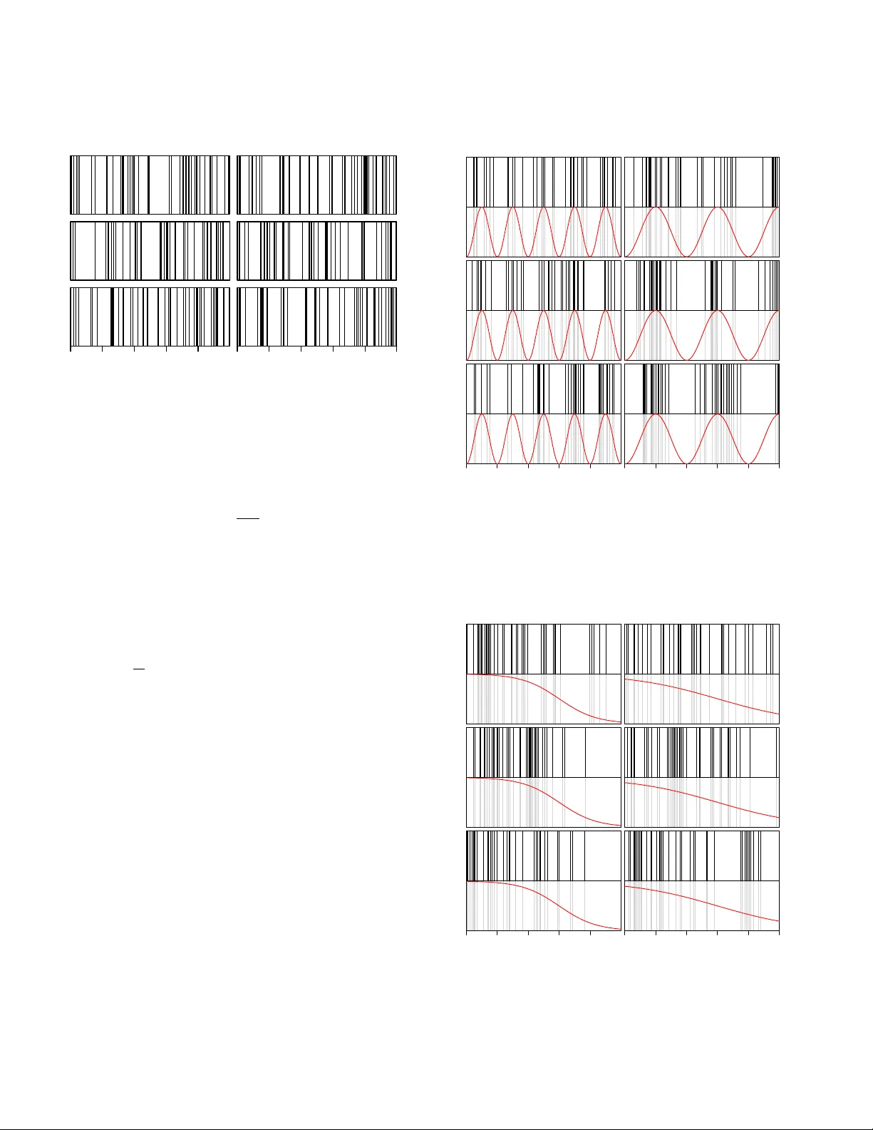
Mon. Not. R. Astron. Soc. 000 , 000–000 (0000) Printed 30 October 2018 (MN L A T E X style file v2.2) Bayesian time series analysis of terr estrial impact cratering C.A.L. Bailer -Jones ∗ Max-Planck-Institut f ¨ ur Astr onomie, K ¨ onigstuhl 17, 69117 Heidelber g, Germany Submitted 13 Mar ch 2011. Revised 11 April 2011 and 17 May 2011. Accepted 20 May 2011. Minor typos corr ected 15 J une 2011. Minor corr ection (err atum) 16 October 2011 ABSTRA CT Giant impacts by comets and asteroids hav e probably had an important influence on ter - restrial biological ev olution. W e know of around 180 high v elocity impact craters on the Earth with ages up to 2400 Myr and diameters up to 300 km. Some studies ha ve identified a periodicity in their age distrib ution, with periods ranging from 13 to 50 Myr . It has further been claimed that such periods may be causally linked to a periodic motion of the solar sys- tem through the Galactic plane. Ho wev er, many of these studies suf fer from methodological problems, for example misinterpretation of p-v alues, overestimation of significance in the pe- riodogram or a failure to consider plausible alternativ e models. Here I dev elop a Bayesian method for this problem in which impacts are treated as a stochastic phenomenon. Models for the time variation of the impact probability are defined and the evidence for them in the geological record is compared using Bayes factors. This probabilistic approach obviates the need for ad hoc statistics, and also mak es e xplicit use of the age uncertainties. I find strong e v- idence for a monotonic decrease in the recorded impact rate going back in time ov er the past 250 Myr for craters larger than 5 km. The same is found for the past 150 Myr when craters with upper age limits are included. This is consistent with a crater preserv ation/discovery bias modulating an otherwise constant impact rate. The set of craters larger than 35 km (so less affected by erosion and infilling) and younger than 400 Myr are best explained by a constant impact probability model. A periodic variation in the cratering rate is strongly disfa voured in all data sets. There is also no evidence for a periodicity superimposed on a constant rate or trend, although this more complex signal would be harder to distinguish. Key words: methods: data analysis, statistical – Earth – meteorites, meteors, meteoroids – planets and satellites: surfaces 1 INTR ODUCTION About 180 terrestrial impact craters are known. The high velocity of the impact means that ev en relatively small comets or asteroids produce large craters. The meteor which crated the 1.2 km diameter Barringer crater in Arizona, for example, was probably only 50m across. Since the discovery of e vidence for a large impact 65 Myr ago at the geological boundary between the Cretaceous and T ertiary periods (the K-T boundary) (Alvarez et al. 1980) and its implication in the mass extinction event at that time (including the demise of the dinosaurs), it has become clear that bolide impacts hav e had a significant impact on the ev olution of life. The large impactors are believed to be either asteroids from the main asteroid belt, or comets from the Oort cloud (Shoemaker 1983). The multi-body dynamics in volved in putting these on a col- lision course with the Earth implies that cratering is a random phe- nomenon, but the rate of impacts is not necessarily constant in time. It has been suggested that gravitational perturbations of the Oort ∗ Email: calj@mpia.de cloud due to the Galactic tide, passages of the solar system near to molecular clouds, or an unseen solar companion, may send large numbers of comets into the inner solar system as a comet sho wer, increasing the impact rate (Davis et al. 1984, T orbett & Smolu- chowski 1984, Rampino & Stothers 1984, Napier 1998, Wickra- masinghe & Napier 2008, Gardner et al. 2011). Simple dynami- cal calculations indicate that the Sun oscillates vertically about the Galactic midplane with a period of 52–74 Myr , depending on the mass density assumed (Bahcall & Bahcall 1985, Shuter & Klatt 1986, Stothers 1998). In parallel to this, several studies claim to hav e found evidence for a temporal periodicity in the impact crater - ing record over the past fe w hundred million years, with numerous periods ranging from 13 to 50 Myr having been identified (Alvarez & Muller 1984, Rampino & Stothers 1984, Grieve et al. 1985, Mon- tanari et al. 1998, Napier 1998, Y abushita 2004, Chang & Moon 2005, Napier 2006). Some authors make a causal link, suggest- ing that each midplane crossing increases the impact rate. It has also been suggested that periodicities in cratering may be associ- ated with alle ged periodicities in mass e xtinctions or in biodiversity variations, although there is little e vidence linking any mass extinc- c  0000 RAS Content is c  C.A.L. Bailer -Jones 2 C.A.L. Bailer-J ones tion apart from the K-T one to a giant impact (Alvarez 2003, Hal- lam 2004; see Bailer-Jones 2009 for a more general revie w of ex- traterrestrial influence on terrestrial climate and biodiv ersity .) Other studies of the crater record conclude there to be insufficient evi- dence for periodicity (e.g. Grieve 1991, Grieve & Pesonen 1996, Y ab ushita 1996, Jetsu & Pelt 2000). While these are a priori reasonable suggestions worthy of fur- ther analysis, many of the studies claiming to have identified peri- ods are compromised by problems with their methodology . T ypical problems are misinterpreting p-values, overestimating the signifi- cance of periodogram peaks, or failing to consider a sufficient set of models. Possibly because the data comprise only crater ages (with no attached magnitudes lik e more familiar time series), many stud- ies have developed ad hoc statistics to look for periods, many of which have poorly explored statistical properties. Identifying “pe- riods” is relatively easy – any time series can be expressed as a sum of Fourier terms; clusters of points can always be found – but properly assessing significance is harder . A common mistake is to interpret evidence against a null hypothesis of “random data” as evidence for some periodic model, neglecting to realise that both may be inferior to a plausible third alternative. Although these are known limitations of frequentist hypothesis testing which have been discussed extensi vely (e.g. Berger & Sellke 1987, Kass & Raftery 1996, Marden 2000, Berger 2003, Jaynes 2003, MacKay 2003, Christensen 2005), this seems not to have discouraged their use. The aim of this article is to analyse the crater time series with well-motiv ated statistical methods. One of the key features is to write do wn explicit models for the impact phenomenon. A second feature is that I consider this phenomenon to be a stochastic pro- cess: Rather than expecting the impact e vents to follow a determin- istic pattern, I model the time variation of the impact probability . This better accommodates the astrophysical and geological con- texts (e.g. smooth variations in the torques on the Oort cloud, or slow erosion of craters). By using the Bayesian frame work to anal- yse the data, we can properly calculate the evidence for the dif ferent models and compare them on an equal footing. The critical aspect is that we must compare evidence for the entire model (the average likelihood over the model parameter space), rather than compar- ing the tuned maximum likelihood fit (which generally fa vours the more complex model). Craters are difficult to date, and some hav e very lar ge age un- certainties (Grie ve 1991, Deutsch & Sch ¨ arer 1994). There has been a lot of agonizing in the literature about how to deal with age uncer- tainties, and some studies may hav e biased their conclusions by re- moving “poor” data. Contrary to claims in the literature, including craters with lar ge uncertainties is not a problem for model compar- ison provided we use these uncertainties appropriately . The method dev eloped in this paper does this, and it can also include craters which only hav e upper age limits. The impact crater record is certainly incomplete. Of most rel- ev ance is the preservation bias: on account of erosion and infilling, older , smaller craters are less likely to survi ve or to be discov ered. The oldest known crater is about 2400 Myr old, but there is an ob- vious paucity of craters older than about 700 Myr (only 14 of 176 older than this). F or this reason I focus my analysis on craters larger than 5 km in diameter which have ages (or upper age limits) be- low 250 Myr , although I also extend the analysis back to 400 Myr BP (before present). Rather than attempting to “de-bias” the data, I model the data as they are, so strictly I am modelling not the orig- inal impact history (which we do not observe), but the combined impact/preservation history . After outlining the data in section 2, I describe the method in section 3. This is tested and demonstrated on simulated data in sec- tion 4. The results are presented in section 5, follo wed by a discus- sion of these and the method and a comparison with other studies in section 6. I summarize and conclude in section 7. I will say very little about the wider topics of the comet and asteroid population, impact ef fects, crater geology and aging etc. These are re viewed by Shoemaker (1983), Grie ve (1991), Deutsch & Sch ¨ arer (1994) and Griev e & Pesonen (1996), amongst others. 2 IMP A CT CRA TER D A T A The data are taken from the Earth Impact Database (EID), a com- pilation from the literature maintained by the Planetary and Space Science Centre at the Uni versity of New Brunswick. 1 This has been the source of data for many previously published studies, and has been continuously expanded as new craters have been discovered, and information revised as improved age or size estimates obtained. As of 30 September 2010 this listed 176 craters. My study fo- cuses primarily on craters younger than 250 Myr with diameters d > 5 km. 59 craters fulfil these criteria and are listed in T able 1. 42 of these hav e an age and age uncertainty in the EID. These uncer- tainties are interpreted as 1 σ Gaussian uncertainties (see section 3.2 for why this is so). The data on the remaining 17 craters fall into three groups: • 13 craters have only upper limits to their ages. These can be included in the analysis consistently , as outlined in section 3.5. • T wo craters, Bosumtwi and Haughton , ha ve no age uncertainty reported in the EID. Craters younger than 50 Myr hav e dating errors ranging from 0.1 to 20 Myr (or 0.3% to 60%), so it is difficult to estimate an appropriate uncertainty . I rather arbitrarily assign 10% uncertainties to the ages of these two craters. • T wo craters, A vak and Jebel W aqf as Suwwan , have age ranges (3–95 Myr and 37–56 Myr respectiv ely) rather than estimates with uncertainties in the EID. I consider the range as a 90% confidence interval of a Gaussian distribution with mean equal to the average of the limits (so the standard deviation is 0.30 times the range). Crater diameters are notoriously dif ficult to measure. No uncertain- ties are listed in the EID, but the uncertainty can be a factor of two or more for b uried craters (e.g. Grie ve 1991). On account of erosion and infilling, the older or smaller a crater is, the less likely it is to be preserved or discovered, resulting in increasing incompleteness with look back time. For this reason – and follo wing several other studies – I limit my analysis to craters larger than 5 km in diame- ter . Our knowledge of geological processes suggests that for times back to 150–250 Myr, most craters larger than 5 km should be rea- sonably well preserved (although this is something I will test). Note that I only use the diameters to select the sample; they are not used in the actual analysis. W e certainly have not identified all impacts: the continents hav e not been explored equally thoroughly , and craters from ma- rine impacts are rarer and harder to identify . But provided these selection effects are time independent (and size independent abo ve 5 km), they do not introduce any rele vant biases. The continents have also moved. 250 Myr, ago at the Permian– T riassic boundary , there was a larger concentration of land mass tow ards southern latitudes than there is now . Giv en that asteroid 1 http://www .passc.net/EarthImpactDatabase/ c  0000 RAS, MNRAS 000 , 000–000 Content is c  C.A.L. Bailer -Jones Bayesian time series analysis of terr estrial impact cratering 3 [h] T able 1. The 59 craters in the Earth Impact Dat abase with diameters greater than or equal to 5 km and ages or age upper limits below 250 Myr Name age σ (age) diameter Myr Myr km Araguainha 244 . 4 3 . 25 40 A vak 49 . 0 28 . 0 12 Beyenchime-Salaatin 40 20 8 Bigach 5 3 8 Boltysh 65 . 17 0 . 64 24 Bosumtwi 1 . 07 0 . 107 10 . 5 Carswell 115 10 39 Chesapeake Bay 35 . 3 0 . 1 90 Chicxulub 64 . 98 0 . 05 170 Chiyli 46 7 5 . 5 Chukcha < 70 6 Cloud Creek 190 30 7 Connolly Basin < 60 9 Deep Bay 99 4 13 Dellen 89 2 . 7 19 Eagle Butte < 65 10 El’gygytgyn 3 . 5 0 . 5 18 Goat Paddock < 50 5 . 1 Gosses Bluff 142 . 5 0 . 8 22 Haughton 39 3 . 9 23 Jebel W aqf as Suwwan 46 . 5 5 . 8 5 . 5 Kamensk 49 0 . 2 25 Kara 70 . 3 2 . 2 65 Kara-Kul < 5 52 Karla 5 1 10 Kentland < 97 13 Kursk 250 80 6 Lappajrvi 73 . 3 5 . 3 23 Logancha 40 20 20 Logoisk 42 . 3 1 . 1 15 Manicouagan 214 1 100 Manson 74 . 1 0 . 1 35 Maple Creek < 75 6 Marquez 58 2 12 . 7 Mien 121 2 . 3 9 Mistastin 36 . 4 4 28 Mjlnir 142 2 . 6 40 Montagnais 50 . 5 0 . 76 45 Morokweng 145 0 . 8 70 Oasis < 120 18 Obolon’ 169 7 20 Popigai 35 . 7 0 . 2 100 Puchezh-Katunki 167 3 80 Ragozinka 46 3 9 Red W ing 200 25 9 Ries 15 . 1 0 . 1 24 Rochechouart 214 8 23 Saint Martin 220 32 40 Sierra Madera < 100 13 Steen Riv er 91 7 25 T in Bider < 70 6 T ookoonooka 128 5 55 Upheav al Dome < 170 10 V ar geao Dome < 70 12 V ista Alegre < 65 9 . 5 W anapitei 37 . 2 1 . 2 7 . 5 W ells Creek 200 100 12 W etumpka 81 1 . 5 6 . 5 Zhamanshin 0 . 9 0 . 1 14 impactors are not distributed isotropically – their orbits are con- centrated in the ecliptic – we may expect this continental drift to introduce a time variation in the impact rate. Ho wever , calculations by Le Feuvre & Wieczorek (2008) show that the impact probabil- ity actually has only a v ery weak latitudinal dependence, being only 4% lower at the poles than at the equator . The net dependence will be ev en lower when (isotropic) comets are included. Thus conti- nental drift produces a very minor bias which I ignore. Fig. 1 shows the ages and diameters of the 46 craters in T able 1 which have age estimates (rather than upper limits). Fig. 2 sho w the ages uncertainties on these points and includes the 13 craters with upper limits on their ages. I perform the analysis on several dif ferent data sets ov er three ages ranges. Craters with age estimates and uncertainties ( σ t ) orig- inating from the EID form the basic data sets. Adding to these the craters for which I hav e assigned ages/age uncertainties forms the extended data sets. Further adding craters with upper age limits ( s up ) giv es the full data sets. I do not make any cut on the age uncertainties. The data sets are as follows basic150 (32 craters) age ≤ 150 Myr , σ t original ext150 (36 craters) age ≤ 150 Myr , σ t original or assigned full150 (48 craters) ext150 plus craters with s up ≤ 150 Myr basic250 (42 craters) age ≤ 250 Myr , σ t original ext250 (46 craters) age ≤ 250 Myr , σ t original or assigned full250 (59 craters) ext250 plus craters with s up ≤ 250 Myr large400 (18 craters) age ≤ 400 Myr , d > 35 km, σ t original This final data set, large400, extends further back in time, but now we definitely expect a bias of preferential preservation and discov- ery for larger craters above 5 km. Follo wing previous studies (see section 6), I therefore just retain craters with much large diame- ters in an attempt to av oid this bias. In addition to the 14 craters matching craters from T able 1, the four additional (older) craters in this set are: Clearwater W est ( 290 ± 20 Myr, 36 km); Charlev oix ( 342 ± 15 Myr, 54 km); W oodleigh ( 364 ± 8 Myr, 40 km); Siljan ( 376 . 8 ± 1 . 7 Myr , 52 km). 3 METHOD I now introduce the time series analysis method, showing ho w to model a generic time-of-arri val data set with a probabilistic model and how to calculate its e vidence. 3.1 Bayesian hypothesis testing The goal of hypothesis testing is to identify which of a set of hy- potheses is best supported by the data. More quantitativ ely , we would like to determine P ( M | D ) , the probability that a hypoth- esis or model M is true giv en a set of measured data D . Here D is the ages for a set of craters. M could be “uniform distribution” or “periodic distribution”, for e xample. Perhaps surprisingly , orthodox (or frequentist) statistics lacks a general framework for this problem and of fers instead a number of recipes based on defining some statistic. These normally inv olve calculating the value for that statistic (e.g. χ 2 ), and comparing it with the value which would be achieved by some “random” (noise) model. As discussed at some length in the literature, some of these techniques are inconsistent or misleading, ev en when we just have two alternativ e hypotheses (e.g. Berger & Sellke 1987, Kass & Raftery 1996, Berger 2003, Christensen 2005, Bailer-Jones 2009; see also section 6). The Bayesian approach, in contrast, is direct and c  0000 RAS, MNRAS 000 , 000–000 Content is c  C.A.L. Bailer -Jones 4 C.A.L. Bailer-J ones 0 50 100 150 200 250 0 50 100 150 Time bef ore present / Myr Diameter / km Figure 1. The 59 craters listed in T able 1, excluding the 13 crater with upper limits on their ages. Several craters ha ve identical or very similar ages so for the sake of this plot I shifted some ages by up to 0.5 Myr in order to distinguish them. ● ● ● ● ● ● ● ● ● ● ● ● ● ● ● ● ● ● ● ● ● ● ● ● ● ● ● ● ● ● ● ● ● ● ● ● ● ● ● ● ● ● ● ● ● ● 0 50 100 150 200 250 5 10 20 50 100 200 Time bef ore present / Myr Diameter / km ] ] ] ] ] ] ] ] ] ] ] ] ] Figure 2. The 59 craters listed in T able 1, including the 13 craters with upper limit ages (plotted with the “]” symbol). There are two upper identical points at 70 Myr , 6 km. The error bars are the age uncertainties and in some cases are smaller than the size of the points. Note that diameter is plotted on a logarithmic scale. often turns out to be quite simple. It inevitably inv olves a number of numerical integrals, but these can be solv ed with computers. For more background on Bayesian techniques in general see Jeffre ys (2000), Jaynes (2003), MacKay (2003) or Gregory (2005). T o calculate P ( M | D ) for one particular model M 0 we use Bayes’ theorem P ( M 0 | D ) = P ( D | M 0 ) P ( M 0 ) P ( D ) = P ( D | M 0 ) P ( M 0 ) k = K P k =0 P ( D | M k ) P ( M k ) = 1 1 + P k = K k =1 P ( D | M k ) P ( M k ) P ( D | M 0 ) P ( M 0 ) (1) where k = 0 . . . K represents all plausible models. If there are only two, M 0 and M 1 , this simplifies to P ( M 0 | D ) =  1 + P ( D | M 1 ) P ( M 1 ) P ( D | M 0 ) P ( M 0 )  − 1 . (2) This follows because implausible models are – by definition – those with ne gligible model prior probabilities, P ( M )  1 . P ( D | M ) is called the e vidence for model M (derived in the ne xt section). If we assign the two models equal prior probabilities, then the evidence ratio alone determines the posterior probability , P ( M 0 | D ) . This evidence ratio is called the Bayes factor B F 10 = P ( D | M 1 ) P ( D | M 0 ) (3) of model 1 with respect to model 0. When B F 10 = 1 the pos- terior probability is 0.5 for both models. When B F 10  1 then c  0000 RAS, MNRAS 000 , 000–000 Content is c  C.A.L. Bailer -Jones Bayesian time series analysis of terr estrial impact cratering 5 P ( M 0 | D ) ' 1 /B F , and when B F 10  1 then P ( M 0 | D ) ' 1 − B F 10 . If we calculate Bayes factors greater than 10 or less than 0.1 then we can start to claim “significant” e vidence for one model ov er the other (e.g. Kass & Raftery 1996, Jeffre ys 2000). I shall use Bayes factors throughout this article to compare models. Giv en the Bayes factors for all models relati ve to M 0 , the pos- terior probability of this model is then P ( M 0 | D ) = " 1 + k = K X k =1 B F k 0 P ( M k ) P ( M 0 ) # − 1 . (4) One dif ficulty of the Bayesian approach is that in order to calculate this posterior probability one must specify all plausible models (in order to get the correct summation needed to normalize the proba- bilities). This is often not possible (other than for simple two-way hypotheses). Y et even when we cannot identify all models, Bayes factors remain a valid way of comparing the relative mer its of a set of models, and thus identifying the best of these. 3.2 Measurement model f or time-of-arrival data The critical characteristic of the crater time series is that it is just a list of times (with uncertainties), without any corresponding quan- tity . This is unlike most other time series encountered in astro- physics, such as a light curves or radial velocity time series. (Some authors have used crater size or inferred impact energy as the “de- pendent variable” in a time series analysis (e.g. Y abushita 2004), but this is risk y given the significant uncertainties in diameters.) Consider a single ev ent j , with measured age s j and corre- sponding uncertainty σ j . This measured age is an estimate of the (unknown) true age, t j . W e express this uncertainty probabilisti- cally . Assuming a Gaussian distribution for the measurement, the probability of observing the measurement s j giv en the true age is P ( s j | σ j , t j ) = 1 √ 2 π σ j e − ( s j − t j ) 2 / 2 σ 2 j (5) which is normalized with respect to s j . 2 3.3 Stochastic time series models The goal is to compare plausible models which could produce the observed impact crater time series. Given the astrophysical conte xt, we do not expect the sequence of crater impacts to be determinis- tic. For example, when we postulate that the time series is “peri- odic”, we do not expect the events to hav e a strict spacing, ev en if the ages were measured arbitrarily accurately . An exact, intrinsic rhythm perturbed only by measurement errors seems highly im- plausible a priori. W e should instead understand periodic to mean a periodically v arying probability of an impact. This is a stochastic model. It is described by P ( t j | θ , M ) , the probability of getting an impact at time t j giv en model M with parameters θ . A simple pe- riodic model would be a sinusoid, described by the two parameters period and phase. 2 The maximum entropy principle tells us that if we only hav e the mean and standard deviation of a quantity , then the least informative (most conserva- tiv e) probability distribution for this quantity is the Gaussian. Of course, if the standard deviation is a significant fraction of the age, then a Gaussian has a significant probabilty mass at negativ e age. As this problem effects no more than five events listed in the table, I consider this as an adequate approximation. P(s 1 | σ 1 , t 1 ) P(t| θ, M) P(s 3 | σ 3 , t 3 ) P(s 2 | σ 2 , t 2 ) time, t Figure 3. Principle of the likelihood calculation (equation 7) 3.4 Bayesian evidence f or time-of-arrival data I now put the above considerations together to derive the Bayesian evidence, P ( D | M ) . The probability of observing data s j from model M with pa- rameters θ is P ( s j | σ j , θ , M ) , the likelihood for one event. The time series model predicts the true age of an ev ent, which is unkno wn. Applying the rules of probability we marginalize o ver this to get P ( s j | σ j , θ , M ) = Z t j P ( s j , t j | σ j , θ , M ) dt j = Z t j P ( s j | σ j , t j , θ , M ) P ( t j | σ j , θ , M ) dt j = Z t j P ( s j | σ j , t j ) P ( t j | θ , M ) dt j . (6) The last step follows from conditional independence: in the first term – the measurement model – once t j is specified s j becomes conditionally independent of θ and M ; in the second term – the time series model – t j is independent of σ j . As the data are fixed, we consider both terms as functions of t j . Both must be properly normalized probability density functions. If we have a set of J e vents for which the ages and uncer- tainties ha ve been esti mated independently of one another, then the probability of observing these data D = { s j } , the likelihood , is P ( D | σ, θ , M ) = Y j P ( s j | σ j , θ , M ) = Y j Z t j P ( s j | σ j , t j ) P ( t j | θ , M ) dt j . (7) where σ = { σ j } . The principle of this calculation is illustrated in Fig. 3: the likelihood of an e vent for a given model is the integral of the probability distribution for the e vent (eqn. 5) over the time se- ries model, P ( t j | θ , M ) . Specific cases for the latter are introduced in section 3.6 below . The evidence is obtained by marginalizing the likelihood o ver the parameter prior probability distribution, P ( θ | M ) , P ( D | σ, M ) = Z θ P ( D, θ | σ, M ) dθ = Z θ P ( D | σ, θ , M ) P ( θ | M ) dθ (8) (where σ drops out of the second term due to conditional indepen- dence). For a giv en set of data (crater time series), we calculate this evidence for the different models we wish to compare, each parametrized by some parameters θ . The parameter prior P ( θ | M ) encapsulates our prior knowledge (i.e. independent of the data) of c  0000 RAS, MNRAS 000 , 000–000 Content is c  C.A.L. Bailer -Jones 6 C.A.L. Bailer-J ones T able 2. Stochastic time series models.Time t increases into the past. Sig- Pr ob:Neg and SigPr ob:P os are special cases of SigPr ob with λ < 0 and λ > 0 respectiv ely . SinPr obX:Y specifies SinPr ob for X < T < Y (in Myr). Name P u ( t | θ, M ) parameters UniProb 1 none SinProb 1 2 (cos[2 π ( t/T + φ )] + 1) T , φ SinBkgProb 1 2 (cos[2 π ( t/T + φ )] + 1) + b T , φ , b SigProb  1 + e − ( t − t 0 ) /λ  − 1 λ , t 0 SinSigProb SinProb + SigProb T , φ , λ , t 0 the probabilitie s of dif ferent parameters, normally established from the context of the problem (see section 3.7). Note that the evidence is dependent on the measurement uncertainties (although I drop this explicit conditioning in the rest of this article). A fundamental aspect of this evidence framew ork for model assessment is that we are not interested in the “optimal” value of the parameters for some model. W e are not interested in “fitting” the model, but rather in determining how good the model is over - all at explaining the data. The evidence measures this by averaging the likelihood, which is defined at fix ed θ , over the prior for θ . The prior probability distribution is therefore important, and should be considered as part of the model definition. For example, a periodic model with a non-zero prior over the period range 10–50 Myr is distinct from a model with a non-zero prior over the range 50– 100 Myr . The reason why we should integrate over the possible solutions rather than selecting the best one will be illustrated and discussed in some detail. 3.5 Inclusion of events with age limits By representing the unkno wn, true age of an event probabilistically , we take into account the age uncertainties. It also allows us to in- clude ev ents which only have upper or lower limits on their ages (censored data). Giv en a (hard) upper limit, s up j , all we know is that the true age is younger . A suitable – and uninformati ve – measurement model is to assume that the probability of measuring some value for the upper limit is constant for any age below the one we actually mea- sured, s up j , and zero otherwise. In this case, we write equation 5 as P ( s up j | t j ) =      1 s up j when 0 < t j < s up j 0 otherwise (9) which is normalized. Recall that time increases into the past. Events which have lower limits to their ages may be treated in the same way , provided we can also assign an upper limit to the pos- sible age (required to normalize the probability density function). It is not obvious how to assign this. W e might use the oldest ev ent in the data set or the age of the oldest rocks searched for craters. As only two e vents with lo wer limits occur in the time ranged analysed (and both quite low , at 35 Myr), these are not included. 3.6 Impact cratering time series models T able 2 lists the time series models which will be tested. The sec- ond column gives the (unnormalized) probability density function that an ev ent occurs at time t for giv en parameters. (For given parameters, these distributions must be normalized over the time span of the data when they are used in the likelihood integral.) Sin- Pr ob is a sinusoid with period T and phase φ . SinBkgPr ob adds a constant background, b , to this. SigPr ob is a sigmoidal function parametrized by the steepness of the slope ( λ ) and the time of the centre of the slope ( t 0 ). It is used to model a monotonic trend in the ev ent probability , with λ < 0 gi ving a decrease in probability with (look back) time. SinSigPr ob models a a periodic signal on top of a trend. Examples of these functions are shown later . 3.7 Choice of parametrization and parameter prior distribution T o calculate the evidence (equation 8) for the models, we integrate ov er the parameters. In order that this integral conv erge we must either adopt a proper prior or , equiv alently , we must adopt a finite parameter range over which the model is defined. In the interests of keeping assumptions limited and the results intuiti ve, I adopt a uniform prior ov er a finite range for all parameters, P u ( θ | M ) = ( 1 when θ min < θ < θ max 0 otherwise (10) The u subscript denotes that this is not normalized (divide by ∆ θ = θ max − θ min to normalize) 3 . It is important to realise that the adopted parameter range is an intrinsic part of the model. Hence, rather than talking about the model SinPr ob , for example, we should talk about the model de- fined ov er some period range. F or this reason I will refer to models like SinPr ob10:50 , which means the SinPr ob model for the period range 10–50 Myr . The e vidence of course also depends on the shape of the prior , and I adopt a uniform prior mostly to represent ignorance. But uni- form over what? It would be equally valid to parametrize the peri- odic models in terms of frequency ( ω = 1 /T ) and adopt a uniform prior o ver that, for example. The transformation between the priors is P T = P ω T − 2 , so a prior uniform in frequency is non-uniform in period. In particular, shorter periods will achie ve more weight in the e vidence calculation. T o assess the impact of this choice, I have repeated all of the analyses described in sections 4 (simulations) and 5 (EID results) which use periodic models with a prior uniform in frequency . It turns out that this change makes bi significant dif- ference to the results, and does not change the conclusions. (The issue of priors is discussed further in section 6.) The ranges for the other parameters are as follows. The phase parameter is only defined in the range 0–1, so it is natural to al ways use this full range (no reason to e xclude any phases). For the back- ground parameter b in SinBkgPr ob , I examine the evidence ov er a range 0–5, the upper limit set by the intuition that with much larger backgrounds it will be hard to detect a periodic signal (this was later gound to be the case). For the parameters of SigProb , I cover the range of λ from 0 to ± 100 . This encompasses models ranging from a step function ( λ = 0 ) to a virtually flat function over the period of interest (see the figures in section 4). The range of t 0 is chosen as 0–275 in order to mov e the “crossing point” of the sigmoid across the whole basic250 time range. 3 Normalization is essential. It ensures that model comple xity is taken into account by the model comparison. Note, therefore, that we are not mod- elling the absolute rate of impacts, just the probability . c  0000 RAS, MNRAS 000 , 000–000 Content is c  C.A.L. Bailer -Jones Bayesian time series analysis of terr estrial impact cratering 7 0 50 100 150 200 0 50 100 150 200 250 Time / Myr Figure 4. Six examples of simulated time series drawn from the model UniPr ob (each with 42 events) 3.8 Numerical estimation The integral in equation 8 is estimated numerically using Z x f ( x ) dx ≈ n = N X n =1 f ( x n ) δ x = ∆ X N n = N X n =1 f ( x n ) (11) where f ( x ) is any continuous inte grable function, the sample { x n } is drawn from a uniform distribution, ∆ X is the range of x from which they are drawn and δ x = ∆ X/ N is the average spacing between the samples. (For equation 7 I just used a regular dense sampling.) P ( θ | M ) = P u ( θ | M ) / ∆ θ = 1 / ∆ θ for all the priors I use, so the numerical integration simplifies to P ( D | M ) ≈ 1 N θ = θ max X θ = θ min P ( D | θ , M ) (12) with the samples drawn from a random uniform distribution. Thus with uniform priors, the evidence is just the likelihood averaged ov er the range of the parameters. This is ev aluated at se veral million randomly selected points, more than enough to ensure a very high signal-to-noise ratio in the calculated evidence. 4 TESTS ON SIMULA TED TIME SERIES T o test the method I apply it to numerous simulated data sets. The goal is to determine whether we can identify the underlying signa- ture in the data, and with what significance, and whether we some- times identify the wrong model. I will demonstrate, for example, that simply identifying a “significant” peak in the periodogram can lead us to the wrong conclusion. I generate stochastic time series using the same probabilistic models described in section 3.6. F or each model and set of parame- ters (e.g. period and phase in SinPr ob ) I dra w ev ents independently at random from the probability distribution. I generate several ran- dom time series for each parameter combination. In all cases a time series comprises 42 events ov er a time span of 250 Myr – charac- teristic of the basic250 data set – and σ t is unity for all ev ents. Figures 4, 5 and 6 sho w example time series drawn from UniPr ob , SinPr ob and SigProb respectively . Note ho w different the time series can be e ven when drawn from the same model with the same parameters. It is also interesting – but not surprising – that stretches of some of the uniform random distribution appear 0 50 100 150 200 0 50 100 150 200 250 Time / Myr Probability (unnormalized) Figure 5. Six examples of simulated time series drawn from the model Sin- Pr ob (each with 42 ev ents). The model is plotted in red, the randomly se- lected e vents in black (in a split panel to aid viewing of these stochastic time series). The model has a period of 50 Myr on the left and 100 Myr on the right (phase = 0.5 in both cases) 0 50 100 150 200 0 50 100 150 200 250 Time / Myr Probability (unnormalized) Figure 6. Six examples of simulated time series drawn from model SigPr ob (each wth 42 e vents). The model is plotted in red, the randomly selected ev ents in black (in a split panel to aid viewing of these stochastic time se- ries). The model has λ = − 30 on the left and λ = − 70 on the right ( t 0 = 150 in both cases) c  0000 RAS, MNRAS 000 , 000–000 Content is c  C.A.L. Bailer -Jones 8 C.A.L. Bailer-J ones almost periodic. Con versely , the time series drawn from SinProb do not always look very periodic. In all cases the distrib ution can be v ery une ven and/or show clustering and gaps. Searching for pat- terns by eye can be quite misleading. I report here just the results of the periodic models using the uniform prior ov er period. The results of using a uniform prior o ver frequency are very similar (I mention a few in the footnotes). Some- times the evidence is higher or lower , but it does not change the strength of any of the conclusions reported. The maximum likeli- hood solutions are, in virtually all simulations, identical in param- eters and likelihood to within 0.1%. 4.1 Periodic data sets I generate data sets from SinPr ob at sev eral different fixed periods and phases. For each time series I calculate the evidence and Bayes factors (e vidence ratios) for a number of models. For the SinPr ob model, the likelihood is calculated at sev- eral million values of period and phase drawn from the uniform prior distribution for periods of 10–550 Myr and phases of 0–1. These likelihoods are plotted as a density plot in Fig. 7 for one particular simulated time series with true period 35 Myr and phase of 0.75 (shown in Fig. 8). There is large variation in the like- lihood. The overall evidence for this model for the full period range 10–550 Myr is found by averaging the likelihoods, and is 8 . 12 × 10 − 101 . The evidence for UniProb is 8 . 89 × 10 − 102 , giv- ing a Bayes factor of 9.1. This is not quite significant according to standard criteria, and would appear to suggest a lack of evidence for the periodic model at first. Howe ver , we hav e searched over a wide range of “periods”: up to twice the time span of the data. W e see in Fig. 7 that these have very lo w likelihoods, bringing down the av erage (the evidence) for SinPr ob . So if we instead average ov er periods of 10–125 Myr then we get an evidence for this “properly periodic” model of 3 . 22 × 10 − 100 , a Bayes factor of 36 relative to UniProb . This is good evidence that the periodic model is the better of the tw o. 4 This is also true for the model ov er intermediate periods: BF( SinPr ob10:250 / UniPr ob ) = 24.5. W e can also calculate the evidence over very narrow ranges of period (for all phases). If we do this for consecuti ve ranges, we get a Bayesian periodogram : the variation of likelihood with pe- riod (or frequency). This is equiv alent to marginalizing the two- dimensional likelihood over phase. It is plotted for the present ex- ample in Fig. 9. As these likelihoods hav e uninterpretable absolute values, I divide (“normalize”) the likelihoods by the evidence of the UniPr ob model. The periodogram gives the Bayes factor of Sin- Pr ob at a specific period (strictly , over a v ery narrow period range) relativ e to UniPr ob , which I denote as BF( SinProb ( t ) / UniPr ob ). W e see a (very) significant peak at just a single period, 34.75 ± 0 . 6 Myr (the uncertainty being the half-width at half max- imum, HWHM). As we have already established evidence for the periodic model ov erall, this indicates that the periodic model at the detected period is a good explanation for these data. 5 The maximum likelihood solution is at a period of 34.5 Myr and a phase of 0.73 Its likelihood is 59 000 times higher than the ev- idence for UniPr ob . This is larger than the peak in the periodogram 4 The evidence for SinProb:10:125 with the uniform frequency prior is 3 . 67 × 10 − 100 , hardly any dif ferent. 5 The peak in the periodogram for model with the uniform frequenc y prior is at 34.64 Myr , and has a BF 86% as large. 50 100 150 200 250 0.0 0.2 0.4 0.6 0.8 1.0 P eriod / Myr Phase −130 −125 −120 −115 −110 −105 −100 Figure 7. Likelihood distribution as a function of period and phase for the SinPr ob model calculated on the simulated data set shown in Fig. 8 (like- lihoods were calculated up 550 Myr, but are only plotted up to 250 Myr .). The logarithm (base 10) of the likelihoods are sho wn on a colour scale: it spans 35 orders of magnitude. White regions are those where the likelihood drops below the minimum plotted. 0 50 100 150 200 250 0.0 0.5 1.0 Time / Myr Probability (unnormalized) Figure 8. A simulated time series (black lines) drawn from SinPr ob with T = 35 Myr and φ = 0 . 75 (red curve) 50 100 150 200 250 0 500 1500 2500 3500 P eriod / Myr BF(SinProb(t)/Uniform) 10 20 30 40 50 0 1000 2000 3000 Figure 9. Bayesian periodogram obtained by marginalizing the 2D likeli- hood distribution in Fig. 7 over the phase. The inset shows a zoom on the 10–50 Myr portion c  0000 RAS, MNRAS 000 , 000–000 Content is c  C.A.L. Bailer -Jones Bayesian time series analysis of terr estrial impact cratering 9 because no w we hav e also found the optimum phase. Howe ver , be- cause this model has two parameters which hav e been fit to the data, this is not a representative measure of the “significance” of a periodic model in which the parameters are not kno wn a priori. This will be discussed further below . This example is actually one in which the simulated time se- ries is relativ ely non-periodic. Many of the random generations pro- duce much more periodic data sets which achiev e peaks in the pe- riodogram of 10 5 or more and a BF( SinPr ob10:125 / UniPr ob ) of hundreds to thousands. The method is very efficient at finding periods in these data sets. Of 100 different random time series drawn from SinPr ob with period 35 Myr and phase 0.5, all 100 showed a (very) significant Bayes factor (relative to UniProb ) for both the overall model ( Sin- Pr ob10:125 ) and at the peak period (which agreed with true period in 99 cases). I obtain very similar results for numerous other time series simulated at other periods and phases: the evidence for the Sin- Pr ob10:125 model is almost always very significant, and there is also always a very strong peak in the Bayesian periodogram. (As one would expect the peak is wider – the period less certain – for longer periods.) The method can also detect periods between 125 and 250 Myr , although periods longer than 250 Myr (where there is less than a complete cycle in the data) are sometimes not detected. Periods do wn to the lowest limit searched for , 10 Myr, can also be recov ered reliably . It must be stressed that the above has only established evi- dence of SinProb relati ve to UniPr ob . In Bayesian hypothesis test- ing we we can only ev er compar e models. I therefore calculated the evidence for the trend model, SigPr ob , defined over the parameter ranges − 100 ≤ λ ≤ +100 , 0 < t 0 < 275 . For the above e xample (Fig. 8), we get a Bayes f actor BF( SinPr ob10:125 / SigProb ) = 155, clearly favouring the periodic model. This is also seen for other simulated time series at the same and other periods: the Bayes fac- tor BF( SinProb / SigPr ob ) is typically 10–1000 for input periods below 250 Myr. For longer periods the SigPr ob model sometimes dominates, depending on the exact data set. This is because such long “periods” are really trends, and these may be fit better with SigPr ob . In conclusion, if the time series is periodic (in the sense of a periodic ev ent probability), then the method strongly fav ours the periodic model over both a uniform one and a monotonic trend model. W e conclude this primarily from the significant (large) Bayes factor for the model as a whole (i.e. a broad period range for all phases), and then from a significant peak in the Bayesian periodogram (the Bayes factor ov er a very narrow period range). 4.2 Uniform and tr end data sets Let us now examine whether we erroneously fav our the SinPr ob model – and possibly detect artificial periods – in non-periodic data. Uniform data sets For this purpose I simulated 50 stochastic time series from the UniPr ob model and calculated the evidence for both UniProb and SinPr ob . In none of these 50 cases is BF( SinPr ob10:125 / UniPr ob ) significant: most of the time series give 10 − 2 to 10 − 3 (the full range is 3 × 10 − 4 to 1.1). BF( SinProb10:250 / UniPr ob ) is like- wise much less than one. W e would therefore correctly conclude that a uniform random distribution is a much better model than a 0 50 100 150 200 250 0.0 0.5 Time / Myr Probability (unnormalized) Figure 10. A simulated time series (black lines) drawn from SigPr ob with λ = − 100 Myr and t 0 = 0 Myr (red curve) periodic one. (If no other model were plausible, we could further conclude with some confidence that this is the “best” model.) Howe ver , in 10 of the cases we nonetheless observe a signif- icant peak in the periodogram at periods less than 125 Myr , where significant means BF( SinProb ( t ) / UniPr ob ) > 10. This is because ev en a uniform random time series with 42 points can happen to show a weak periodicity at some period, even though the periodic model overall is a poorer explanation for the data than the uniform one. 6 If we took just the identification of these “significant” peaks to be e vidence for a period (as is done in frequentist periodogram analyses), we would make a false positiv e claim in 20% of cases. This underlines the importance of basing a conclusion on the evi- dence for the model as a whole, rather than a specific fit. T r end data sets W e see the same general phenomena among a set of time series generated from SigPr ob : The evidence for SinPr ob10:125 is much lower than the evidence for SigPr ob , leading us to correctly con- clude a lack of evidence for periodicity . But once again there are spurious “significant” peaks in the periodogram. The reason for this is that although SinProb sometimes giv es high evidence at a very specific period, once av eraged over a broader period the evidence is much less. If the peak had been much higher (as w as the case for the truly periodic data sets above, e.g. Fig. 9), then av eraging over a broader period reduces the evidence, b ut not enough to make it insignificant. The model evidence is a balance between the quality of a specific fit, and how much of the parameter space produces a good fit. (This is discussed further in section 6, where it can be un- derstood in terms of Occam factors). As we had no prior reason to suspect a periodicity at the peak found , it is misguided to focus only on that peak – and that may anyway giv e the wrong conclusion, as we hav e just seen. An example time series drawn from the trend model is sho wn in Fig. 10. The likelihood distribution for the SigPr ob model is shown in Fig. 11, with a colour scale spanning 15 orders of mag- nitude. Positi ve trends (probability increasing with look back time) are heavily disfav oured. In contrast, a very broad range of param- eter space for λ < 0 has large evidence: the model is not very sensitiv e to the exact parameters. This contrasts with the simulated periodic data sets, where the evidence for the overall model came from a very narrow range of the parameters with very high likeli- hood (see Figs 7 and 9). 6 Half of the time series in fact show a peak in the periodogram with BF( SinPr ob ( t ) / UniProb ) in the range 1 to 10. W e clearly must resist the temptation to read too much into such low significance peaks! c  0000 RAS, MNRAS 000 , 000–000 Content is c  C.A.L. Bailer -Jones 10 C.A.L. Bailer-J ones 0 50 100 150 200 250 −100 −50 0 50 100 tzero / Myr lambda −110 −108 −106 −104 −102 −100 −98 Figure 11. Log likelihood distribution as a function of λ and t 0 in the Sig- Pr ob model calculated for the simulated data set shown in Fig. 10. The log(Evidence) for the overall model is − 97 . 8 (and 0.3 higher for Sig- Pr ob:Neg ). F or comparison, log(Evidence) = − 100 . 9 for UniPr ob . It is interesting to note that the evidence for SinPr ob10:125 on these trend data sets is low even when compared to UniPr ob : The Bayes factors range from 0.7 to 5 × 10 − 5 in 39 of 40 simulations (the other v alue was 2). So even when comparing against an o verly simple model, we get no evidence for periodicity . Y et the in the periodograms normalized to the evidence in UniPr ob we see ap- parently significant peaks, i.e. with BF( SinPr ob ( t ) / UniPr ob ) > 10. These peaks are irrelevant, howe ver , not only because SinPr ob as a whole is disfavoured but also because UniPr ob is a poor model for the data. That is, we can increase the appar ent significance of a model (here SinPr ob ) by comparing it with an ov erly-simple al- ternativ e model (here UniProb ), a common mistake in hypothesis testing. 4.3 Compound data sets It is plausible that the impact cratering phenomenon comprises both a periodic and a non-periodic component (e.g. Grieve et al. 1988, L yytinen et al. 2009). It is generally more difficult to identify evi- dence for more complex models gi ven a limited amount of data and the stochastic nature of the phenomenon. This difficulty is confirmed by simulations. I simulated 48 time series drawn from SinBkgPr ob for sev eral periods between 10 and 250 Myr and b = 1 , i.e. equal amplitudes of the periodic and uniform components (T able 2). In many cases the evidences for SinBkgProb10:550 , SinBkgPr ob10:125 and UniPr ob are about equal, so the true model is not fav oured over a pure “background” model. ( SigPr ob achie ves a very low evidence in comparison: we do not erroneously claim a trend when there is not one.) W e see much the same for sev eral time series drawn from Sin- SigPr ob at each of three different periods (20, 35, 50 Myr) with a fixed trend ( λ = − 60 , t 0 = 100 ). The Bayes factors of the true models relative to just the trend models, SigProb , lie between 0.5 and 7. 7 Thus although the true model is not explicitly disfa voured, these values are not high enough to claim significant evidence to fa vour it, and when lacking e vidence in fav our of a more complex model, we would probably prefer the simpler one. It seems that the method is conservati ve, ha ving difficulties to identify a period in a stochastic time series which includes a large (here 50% amplitude) non-periodic component. A similar conclu- sion was reached by L yytinen et al. (2009) using a different ap- proach. Howe ver , I have only performed a few tests with these compond data sets, and only for a very narrow part of the input parameter space. As the sensitivity is likely to v ary ov er the input parameter space, more extensi ve tests are necessary . In conclusion of this section on simulations, I have found that if the time series is a stochastic one drawn from a model with a periodic distribution, then there is both significant evidence for periodicity and we can identify the true period. Con versely , if data are drawn from a uniform or trend distribution, we find significant evidence for the correct model, and do not erroneously identify periodic- ity . Preliminary tests indicate dif ficulty in favouring more comple x compound models (when true) over a simpler one. It may be that 42 ev ents is simply inadequate to support more complex models. 5 RESUL TS Armed with the experience of how the models respond to time se- ries of kno wn origin, I no w turn to analysing the real cratering data. For quick refefence, the results are summarized in T able 3. For the periodic models I only report results using a prior uniform over pe- riod, because the results for using a prior uniform over frequency are the same in all relev ant respects. An example is shown in the appendix. I should point out that although I calculate likelihoods for the periods models for periods up to twice the time span, I do this only to illustrate that long “periods” can only really be interpreted as long-term trends, and so are better modelled by the SigProb model. The main results for “periodicity” are for the evidence calculated ov er narrower period ranges. 5.1 Data sets: basic150 and ext150 I start with the basic150 data set, the 32 craters o ver the past 150 Myr . The likelihood distribution for the SinProb model is shown in Fig. 12. The evidence for SinProb10:300 is 9 . 64 × 10 − 72 . This compares to 1 . 63 × 10 − 70 for the UniPr ob model, giving a Bayes factor of 0.060, or significant evidence in f avour of UniPr ob . The maximum likelihood over this parameter range occurs at (pe- riod, phase) = (11 . 7 , 0 . 73) with a likelihood of 8 . 00 × 10 − 69 , or BF( SinPr ob ( t ) / UniPr ob ) = 49. Although this tells us that this very specific fit explains the data better than a uniform random distri- bution, it only comes about because we ha ve tuned two parameters (period and phase). UniProb has no free parameters and cannot be tuned, so a simple comparison of maximum likelihood does not take into account the model complexity . This is why we must use the evidence for the models as a whole. After all, we wanted to look for e vidence of periodicity in general, not for evidence of “a period of 11.7 Myr and phase 0.73”, and more complex models could be defined which for which there are ev en higher likelihood fits. 7 When using a uniform prior over frequency the Bayes factors come out to within about 20% of the same values. c  0000 RAS, MNRAS 000 , 000–000 Content is c  C.A.L. Bailer -Jones Bayesian time series analysis of terr estrial impact cratering 11 T able 3. The evidence (equation 8) for dif ferent models and data sets. The Bayes factor is the ratio of two evidences (for a gi ven data set). See the text for the exact parameter ranges used in each case. basic150 full150 basic250 ext250 full250 large400 UniProb 1 . 63 e − 70 2 . 30 e − 105 1 . 03 e − 103 1 . 68 e − 113 3 . 27 e − 145 1 . 25 e − 47 SinProb10:50 2 . 67 e − 71 1 . 41 e − 105 2 . 87 e − 104 1 . 11 e − 113 4 . 83 e − 145 8 . 89 e − 48 SinProb10:125 1 . 07 e − 71 5 . 56 e − 106 1 . 15 e − 104 4 . 18 e − 114 1 . 71 e − 145 1 . 01 e − 47 SinProb10:300 9 . 64 e − 72 SinProb10:400 3 . 35 e − 48 SinProb10:550 8 . 57 e − 103 SinBkgProb10:50 1 . 62 e − 70 1 . 11 e − 103 2 . 23 e − 113 5 . 22 e − 145 SinBkgProb10:125 1 . 58 e − 70 9 . 71 e − 104 1 . 79 e − 113 3 . 91 e − 145 SinBkgProb10:300 1 . 74 e − 70 SigProb 1 . 35 e − 70 1 . 28 e − 103 8 . 64 e − 102 1 . 21 e − 110 7 . 66 e − 139 2 . 93 e − 48 SigProb:Neg 2 . 64 e − 70 2 . 56 e − 103 1 . 73 e − 101 2 . 41 e − 110 1 . 53 e − 138 4 . 83 e − 48 SigProb:Pos 5 . 70 e − 72 3 . 73 e − 108 1 . 47 e − 106 8 . 72 e − 117 3 . 01 e − 149 1 . 03 e − 48 SinSigProb 6 . 94 e − 102 6 . 81 e − 111 7 . 97 e − 140 50 100 150 200 250 300 0.0 0.2 0.4 0.6 0.8 1.0 P eriod / Myr Phase −90 −85 −80 −75 −70 Figure 12. Log likelihood distrib ution as a function of period and phase for the SinPr ob model for the basic150 data set Limiting the evidence calculation to shorter periods of 10– 50 Myr, we get a Bayes f actor of SinPr ob10:50 relati ve to UniPr ob of 0.16, still insignificant evidence for periodicities. The Bayesian periodogram (section 4.1) is shown in Fig. 13. There is no significant evidence for periodicity at any period. Recall that, in the simulations, we obtained a peak (at the true period) with far higher Bayes factors (significance) when the data were drawn from a sinusoidal probability distribution. In the appendix I repeat this analysis using a prior uniform in frequency for SinPr ob . If the impact history comprises both constant and periodic components, then a model which reflects this may identify a pe- riodicity better . T o examine this I calculate likelihoods for SinBkg- Pr ob , which adds a variable constant background term, b , to Sin- Pr ob . For the full period range and for 0 ≤ b ≤ 5 the evidence is 1 . 74 × 10 − 70 , a Bayes factor relati ve to UniProb of 1.1. If we limit the period range to 10–50 Myr this rises only to 1.2. The pe- 0 50 100 150 200 250 300 0 1 2 3 P eriod / Myr BF(SinProb(t)/Uniform) 10 20 30 40 50 0 1 2 3 Figure 13. Bayesian periodogram for the SinPr ob model for the basic150 data set riodogram shows smaller Bayes factors than in Fig. 13, ev en when calculated for limited ranges of b . Hence SinBkgPr ob describes the data no better than a purely uniform random distrib ution, which we should arguably then prefer (see section 6). So far the uniform random distribution describes the data as well as or better than a periodic one. This does not mean that this is the best model, howe ver: we can only assess what we ex- plicitly test. T o look for the evidence for a trend in the data, I calculate the evidence for the SigPr ob over the parameter range − 100 ≤ λ ≤ +100 , 0 < t 0 < 150 . This giv es 1 . 35 × 10 − 70 , a Bayes factor relative to UniPr ob of 0.83. Splitting SigPr ob into two distinct models, one for λ < 0 ( SigPr ob:Ne g ) and the other for λ > 0 ( SigPr ob:P os ), the Bayes factors are 1.63 and 0.035 respec- tiv ely . The latter – an increase in impact probability with look back time – is disfa voured. Performing the same analyses on the ext150 data set giv es very similar results: Adding these four ev ents does not make the evidence for periodicity nor for a trend significant. In summary , we have no evidence for periodicity in the ba- sic150 or ext150 data sets. Of the models tested, both UniPr ob and SigProb:Ne g are more or less equally probable explanations. c  0000 RAS, MNRAS 000 , 000–000 Content is c  C.A.L. Bailer -Jones 12 C.A.L. Bailer-J ones Giv en a lack of strong e vidence in fav our of the more complex trend model, I conclude that the simpler , uniform random distribution is an adequate – and plausible – explanation for impact craters over the past 150 Myr . 5.2 Data set: full150 I no w add the 12 craters which ha ve upper ages limits below 150 Myr, using the approach explained in section 3.5. The evidence for the models tested (same parameter ranges for basic150) are listed in T able 3. There is now significantly more e vidence for the trend model than for the uniform one. More specifically , the nega- tiv e trend ( SigPr ob:Ne g ) is hugely fav oured over the positive one. 8 As the new data are upper age limits, it is not surprising that their inclusion increases the evidence for SigPr ob:Neg , although the ev- idence is very strong: BF( SigPr ob:Neg / UniPr ob ) = 111. Thus adding the 12 craters with upper age limits in a conserva- tiv e manner (a flat probability distribution) has made SigProb:Ne g much more probable than UniPr ob . SinPr ob remains unlikely . Let us now e xtend the data set back to 250 Myr BP . 5.3 Data set: basic250 This data set comprises 42 events. The evidence for UniProb is 1 . 03 × 10 − 103 compared to 8 . 57 × 10 − 103 for SinPr ob10:550 , a Bayes factor of 8.3. The top-left panel of Fig. 14 shows the like- lihood distribution. The largest likelihoods are in the upper right quadrant, for periods greater than 200 Myr and phases above 0.5. Indeed, the maximum likelihood solution is at a period of 550 Myr with a phase of 0.94: it is plotted in the top-right panel of the same figure. This “period” is twice the duration of the data and is ac- tually modelling a trend of decreasing probability with look back time. Marginalizing the likelihood distribution over all phases to produce the periodogram (Fig. 15), we see that all of the significant periods are at these very long trend periods. The evidence for true periods – SinPr ob10:125 – is 1 . 15 × 10 − 104 , a B ayes factor relati ve to UniPr ob of 0.11. Giv en that the likelihood varies considerably across the pa- rameter space, it is informative to examine the model at various pa- rameter “solutions”. Fiv e examples are shown in Fig. 14. The two panels in the central ro w hav e the same period but different phases: the right-hand one giv es an increasing probability of events with look back time and is hugely disfav oured by the data compared to the decreasing trend. The lower two panels are local maxima in the likelihood distribution at shorter periods. They look as though they could reasonably produce the observed data, bearing in mind that these are stochastic models. Howe ver , ev en the better of the two has a likelihood 10–100 times smaller than the longer period “trend” solutions. Introducing a constant background into the model ( SinBkg- Pr ob ), we again find that the highest likelihood solutions (and the only ones more likely than UniPr ob ) are at long “periods”. Solu- tions with b > 0 . 5 are fa voured compared to those with a smaller (or zero) background. There is no evidence for any proper period ( < 125 Myr), with Bayes factors relative to UniPr ob of no more than 0.94, even if we examine narrow ranges of b . So there is no evidence for periodicity superimposed on a constant background 8 As the evidence for SigPr ob is the av erage of the evidence for its two components, and one is fiv e orders of magnitude smaller than the other, then the evidence for SigPr ob:Neg is just twice that of SigPr ob . probability (although recall from section 4.3 that it may be hard to identify such a model with confidence). Giv en the above evidence for a trend, I fit SigPr ob over the parameter range − 100 ≤ λ ≤ +100 , 0 < t 0 < 275 . The overall evidence is 8 . 64 × 10 − 102 . This includes both positive and negati ve trends: Fig. 16 shows that the former ( λ > 0 ) hav e much lower likelihoods. Splitting this model into two, we find that the e vidence for λ < 0 ( SigPr ob:Neg ) is 1 . 73 × 10 − 101 , a Bayes factor of 167 relativ e to UniPr ob . As SigProb:Ne g is much more plausible than UniProb , this tells us that UniProb is an inappropriate reference model for the periodogram in Fig. 15. By comparing the evidence at each pe- riod to a model which predicts the data poorly , the periodic model may of course look good in comparison. But this is not the same as saying that the period is significant, because other (plausible) models may predict the data e ven better , as is the case here. This mistake is often made when assessing the significance of the clas- sical (e.g. Lomb–Scargle) periodogram. One must be careful to choose an appropriate “background” or “reference” model for com- parison. When using the evidence for SigProb:Ne g as the refer- ence in the periodogram, the Bayes factors in Fig. 15 are all re- duced by a factor of 167, rendering all peaks – and even the long “trend” periods – entirely insignificant. Overall, the neg- ativ e trend model is far more probable than the periodic one: BF( SigPr ob:Ne g / SinProb10:125 ) = 1500. Not only is SigPr ob:Neg the fa voured model, it also has a lar ge likelihood over a wide range of t 0 and λ . In other words, the evi- dence is not very sensiti ve to the exact parameter settings (nor to the prior). This can be seen in Fig. 17: half of the parameter space below λ = 0 has a lik elihood within a factor of 10 of the maximum. (The model has a lar ge Occam f actor: see section 6) The maximum likelihood solution is plotted ov er the data in Fig. 18. Because the likelihood peak is so broad, we should not (need not) attrib ute much significance to this specific solution. Is there evidence for a periodicity on top of this trend? W e examine this using the four-parameter model SinSigProb using the same parameter range adopted for the periodic and trend models (namely all phases, periods of 10–125 Myr , − 100 ≤ λ < 0 and 0 < t 0 < 275 ). The evidence is 6 . 94 × 10 − 102 , a Bayes factor with respect to SigPr ob:Neg of just 0.40. If we reduce the parameter range, e.g. to 10-50 Myr, λ < 25 and t 0 < 200 , then the evidence hardly changes. W e could possibly identify narrow , isolated re gions of parameter space where SinSigPr ob is more probable, b ut this has no justification. In summary of the basic250 data set, we have found signifi- cant evidence for a trend of decreasing probability of cratering with lookback time relativ e to both constant and periodic models. This is about the simplest model we can conceiv e after the constant one, and it also has more evidence than a model with a periodicity su- perimposed on either a trend or a constant background probability . 5.4 Data set: ext250 If I add the four craters for which I assigned age uncertainties, the evidence for the trend model relative to both the uniform model and the periodic models increases significantly (see T able 3; the parameters for SinSigPr ob are the same as used for basic250). This is not surprising because the additional craters are all comparati vely young (1.07, 39, 46.5, 49 Myr). c  0000 RAS, MNRAS 000 , 000–000 Content is c  C.A.L. Bailer -Jones Bayesian time series analysis of terr estrial impact cratering 13 100 200 300 400 500 0.0 0.4 0.8 P eriod / Myr Phase −125 −120 −115 −110 −105 + + + + + 0 50 100 150 200 250 Period = 549.96 Phase = 0.94 L = −100.33 Time / Myr 0 50 100 150 200 250 Period = 400.00 Phase = 0.80 L = −100.95 Time / Myr 0 50 100 150 200 250 Period = 400.00 Phase = 0.40 L = −138.19 Time / Myr 0 50 100 150 200 250 Period = 34.50 Phase = 0.85 L = −101.56 Time / Myr 0 50 100 150 200 250 Period = 80.00 Phase = 0.20 L = −102.32 Time / Myr Figure 14. The top-left panel shows the log likelihood distribution as a function of period and phase for the SinPr ob model for the basic250 data set. The red curves in the five other panels show fiv e possible “solutions” at five ( T , φ ) values corresponding to the fiv e crosses plotted on the likelihood distribution. The black lines are the basic250 data. The log (base 10) likelihood and parameters of each solution are given at the top of each panel. The top-right panel is the maximum likelihood solution. The bottom left-panel is (close to) the maximum likelihood solution for short periods. For comparison, log(Evidence) for UniPr ob and SigProb:Ne g are − 102 . 99 and − 100 . 76 respectively . 5.5 Data set: full250 I now add the 13 craters with upper age limits, noting that 12 of them are below 150 Myr . As they are upper age limits, it is not surprising that their inclusion increases the evidence for Sig- Pr ob:Ne g further . But the increase is enormous: the e vidence is 1 . 53 × 10 − 138 compared to 3 . 27 × 10 − 145 for UniPr ob , a Bayes factor of 4 . 7 × 10 6 . The e vidence for SinPr ob10:125 is very small, gi ving a negli- gible Bayes factor relati ve to SigPr ob:Neg . The highest peak in the periodogram is still around 35 Myr, but its evidence is 10 5 times smaller than the evidence for SigPr ob:Ne g . Modelling the data us- ing a periodicity on top of a trend – with SinSigProb – increases the evidence for proper periods (i.e. below 125 Myr) dramatically ov er using just SinPr ob . But they are still insignificant compared to a pure trend. For example, the evidence for SinSigPr ob ov er pe- riods of 10–50 Myr and λ < 0 is 7 . 97 × 10 − 140 , a Bayes factor of 0.052 relative to SigPr ob:Ne g . All peaks in the periodogram are also insignificant. The data are better described with a pure trend. In summary , adding the 13 craters with only upper age limits radically increases the evidence for a negati ve trend, and radically decreases the evidence for either a periodicity or a periodicity plus negati ve trend, relati ve to the simple negati ve trend. 5.6 Data set: large400 The trend detected in the previous data sets might reflect a preser- vation bias in the geological record. When extending the anal- ysis to older craters we can try to a void this bias by only in- cluding larger craters. The large400 data set comprises 18 craters larger than 35 km with ages up to 400 Myr . The Bayes factor BF( SinPr ob10:400 / UniPr ob ) is 0.27. W e see several low peaks in the periodogram, the four highest being 34 Myr (BF = 6.5), 18 Myr and 13.5 Myr (both BF = 5.5), and 100 Myr (BF = 4). As there is no prior reason to expect a period at any of these, we cannot sim- ply select one and claim it as evidence (albeit marginal) for that period, especially giv en that there are so many low peaks (and only 18 data points). Again we must look at the overall e vidence for periodicity . For the period range 10–50 Myr the Bayes factor c  0000 RAS, MNRAS 000 , 000–000 Content is c  C.A.L. Bailer -Jones 14 C.A.L. Bailer-J ones 0 100 200 300 400 500 0 10 20 30 40 50 P eriod / Myr BF(SinProb(t)/Uniform) 10 20 30 40 50 0 1 2 3 4 5 6 Figure 15. Bayesian periodogram for the SinPr ob model for the basic250 data set. If we normalize the periodogram against model SigPr ob:Neg in- stead of the UniProb then the Bayes factors are reduced by a factor of 167. 0 50 100 150 200 250 −100 −50 0 50 100 tzero lambda −140 −130 −120 −110 + + Figure 16. Log likelihood distrib ution as a function of λ and t 0 for the Sig- Pr ob model for the basic250 data set. The black cross marks the maximum likelihood solution. 0 50 100 150 200 250 −100 −50 0 tzero lambda −101.2 −101.0 −100.8 −100.6 −100.4 + + Figure 17. As Fig. 16 but only for λ < 0 and with a shallower likelihood scale to better show the re gion around the peak. 0 50 100 150 200 250 0 1 Time / Myr Probability (unnormalized) Figure 18. The maximum lik elihood solution of SigPr ob (red curve) for the basic250 data set (black lines). It has λ, t 0 = ( − 75 , 98) and a likelihood of 6 . 04 × 10 − 101 . BF( SinPr ob10:50 / UniPr ob ) is 0.71, implying that the periodic and uniform models describe the data equally well. But the periodic model with two free parameters for a pre-defined period range is arguably much less plausible a priori. There is also no evidence for a positiv e or negati ve trend in the data, with Bayes factors below 0.4 for the SigPr ob models (see T able 3). In summary , the large400 data set is most plausibly described by UniPr ob . Let us now turn to a discussion of the complete set of results as well as the method and principles on which it is based. 6 DISCUSSION I have found significant e vidence for a decrease in the cratering rate with lookback time (model SigPr ob:Neg ) over the past 250 Myr for d > 5 km craters relative both to periodic models ( SinProb , Sin- BkgPr ob , SinSigPr ob ) and to a model with constant rate ( UniPr ob ). As there is no strong evidence for a trend in the past 150 Myr, this must come about primarily from a comparati ve lack of events be- tween 150 and 250 Myr BP . This may now seem obvious from Figs. 1 and 2, but the analysis quantifies this and has also taken into account the age uncertainties. No such trend is found for lar ger craters (d > 35 km) over the past 400 Myr . These results could be explained by a decreasing probability of preserv ation/discovery for older craters of size 5–35 km. How- ev er, studies of lunar cratering suggest that the cratering rate during the past 500 Myr was about twice as high as the average over the past 3.3 Gyr (e.g. Shoemaker 1983). More immmediately relev ant is the study of McEwen et al. (1997), who concluded that the cra- tering rate has increased up to the present by a factor of two during the past 300 Myr . If correct, and if the Earth is assumed to have experienced the same bombardment history , then this is consistent with my inferred increase of impact probability from 250 Myr BP up to the present. The single most probable solution for the trend model is shown in Fig. 18. These conclusions are obviously based on the data we cur- rently have. It is quite possible that a significant revision of the ages or the age uncertainties, or the inevitable discov ery of more craters in the future, will lead us different conclusions based on c  0000 RAS, MNRAS 000 , 000–000 Content is c  C.A.L. Bailer -Jones Bayesian time series analysis of terr estrial impact cratering 15 the same analysis. More craters may permit a better distinction be- tween more complex models. I will no w discuss some aspects of the method, and compare the present analysis with previous w ork. Significance assessment. The significance of a model can only be assessed relativ e to the significance of some other model. There is no absolute. In frequentist statistics one normally selects some “noise” or “background” model against which to compare a statis- tic measured on the real data. For example, with the classical peri- odogram the significance is usually determined from the distribu- tion of the power achiev ed by a noise model. This may indicate that the periodic model is the better of the two, but both might be bad: there may be a third model which is better still. W e saw an example of this in Fig. 14, where the bottom left-hand panel is the best-fit truly periodic solution. It was significant relative to UniPr ob , but insignificant relativ e to SigPr ob:Neg . Why we should not rely solely on periodogram peaks. As has already been demonstrated in section 4, reliance on observing a peak in the periodogram – e ven when normalized to the true model – often results in erroneously claiming the periodic model to be a better explanation than the true one. The reason is that the peri- odogram has one free parameter (period), and we can sometimes find a specific value of this parameter which produces a better fit than the simpler uniform model (which has no free parameters). A model with ev en more free parameters may fit better still. But a model with fitted parameters is a priori less plausible than a model with no fitted parameters. Unless we hav e independent information to assign the model parameters, we cannot fit them and then com- pare that model on an equal footing with a model which has not been fit. Instead we must compare models “as a whole” (e.g. over some period range). W e saw an example of this in section 4.2. Occam factor . The conclusion of the previous discussion is not that more complex models are always penalized. They are not. What counts is how the plausibility of the model is changed in light of the data. This can be understood by the concept of the Occam factor . If the likelihood function is dominated by a single peak, then we can approximate the evidence (equation 8) with P ( D | M ) | {z } Evidence = L ( ˆ θ ) | {z } best fit likelihood × ∆ θ posterior ∆ θ prior | {z } Occam factor (13) where L ( ˆ θ ) is the likelihood at the best fit solution, ∆ θ prior is the prior parameter range and ∆ θ posterior is the posterior param- eter range (the width of the likelihood peak) (see, e.g. MacKay 2003). The Occam factor (which is always less than or equal to one) measures the amount by which the plausible parameter vol- ume shrinks on account of the data. For given L ( ˆ θ ) , a simple or general model will fit over a large part of the parameter space, so ∆ θ prior ∼ ∆ θ posterior and the Occam factor is not significantly less than one. W e saw an example of this in Fig. 17. In contrast, a more complex model, or one which has to be more finely tuned to fit the data, will ha ve a larger shrinkage, so ∆ θ posterior  ∆ θ prior . W e saw this for the periodic models at short periods (e.g. Figs. 14 and 15), in which only a very specific period was a good fit to the data. In this case the Occam factor is small and the evidence is re- duced. Of course, if the fit is good enough then L ( ˆ θ ) will be large, perhaps lar ge enough to dominate the Occam factor and to gi ve the model a large evidence. W e saw this with the simulated periodic time series for the SinPr ob model (Fig. 9). This concept helps us to understand how the Bayesian ap- proach accommodates model complexity , something generally lacking in frequentist approaches. If we assess a model’ s evidence only by looking at the maximum likelihood solution (or the maxi- mum o ver one parameter, the period), then we artificially compress the prior parameter range, increasing the Occam factor . Parameter prior distributions. As the model e vidence is the like- lihood av eraged over the prior parameter range (for uniform priors), this raises the issue of what this range should be. This is often the main perceived difficulty with Bayesian model comparison, and for some people this dependence on prior considerations is undesir- able. Y et it is both logical and fundamentally una voidable, because Bayesian or not, the prior parameter range is an intrinsic part of the model. Changing the parameter range changes the model, so will change the evidence. SinPr ob10:50 is totally different from SinPr ob100:150 , for example. If we are comfortable with decid- ing which are the plausible models to test, we must also be willing to decide what are the plausible parameter ranges to test. T o some extent we can be guided by the conte xt of the problem and the gen- eral properties of the data or the experiment, such as the sensiti vity limits. For periodic models it seems obvious that we should use the whole phase range and that we should not include at “periods” much larger than the duration of observations (as these are more like trends). For SigPr ob I hav e actually used a rather broad range of its two parameters, e ven though some of this parameter space is a priori implausible, e.g. λ = 0 gives a probability of zero to one side of t 0 = 0 . More generally , the evidence is the likelihood averaged over the parameter prior distribution. There are often cases where we would not want to use a uniform distribution. It can be difficult to choose the “correct” prior distribution, and this choice may affect the results. Y et whether we like it or not, interpreting data is a sub- jectiv e business: Just as we choose which experiments to perform, which data to ignore, and which models to test, so we must decide what model parameters are plausible. This seems preferable to ig- noring prior kno wledge or, worse, to pretending we are not using it. In general, a probability density function is not in variant with respect to a nonlinear transformation of its parameters. As already discussed in section 3.7, I could equally well have used frequency rather than period to calculate the evidence for periodic models: there is no “natural” parameter here. This would not change the error model of the data (eqn. 5), and the value of P ( t j | θ , M ) at period T is the same as when calculated at frequency 1 /T , so the likelihoods are unchanged. But as the model e vidence is the average of the lik elihoods over the prior, then the evidence w ould change if we adopted a prior which is uniform over frequency rather than ov er period. Thus the choice of parametrization becomes one of choice of prior . As neither parametrization is more natural than the other – a prior uniform over frequency does not seem to be more correct than one uniform over period – this remains a somewhat arbitrary choice. F or this reason I repeated all of the analyses using periodic models with a prior uniform in frequency . Sometimes the evidence was slightly higher, sometimes lo wer, but the significance of the Bayes factors was not altered. The conclusions are robust to this change of prior/parametrization. Model priors. I have used Bayes f actors to compare pairs of mod- els. Models are treated equally , so a significant de viation from unity giv es evidence for one model over the other . Howe ver , if the mod- els have dif ferent complexities (or rather, dif ferent prior plausibili- c  0000 RAS, MNRAS 000 , 000–000 Content is c  C.A.L. Bailer -Jones 16 C.A.L. Bailer-J ones ties) and the Bayes factor is unity , then rather than being equivocal we may tend to prefer the simpler model. This is because we nor- mally gi ve the less plausible model a lower model prior probability (equation 2). W e can include these priors by reporting instead the posterior odds P ( D | M k ) P ( D | M 0 ) P ( M k ) P ( M 0 ) = B F k 0 P ( M k ) P ( M 0 ) . (14) It is not obvious that all of the models I hav e considered should hav e equal model priors. For example, SinSigProb is arguably less plausible than SigPr ob a priori. Posterior probabilities and plausible models. Ideally we would calculate model posterior probabilities, P ( M | D ) . This can only be done if we calculate the e vidence for all plausible models, those with P ( M ) which is not vanishingly small. In the current problem I have conceiv ably included most of the plausible param- eter space for the stated models: These non-deterministic mod- els are quite flexible in describing general shapes. For example, I found that a model with periodic Gaussians (with three param- eters) looked very similar to SinPr ob . (Giv en sufficient physical reason, we could of course define more complex models, e.g. with a variable period or amplitude.) Assuming that SigPr ob:Neg , Sig- Pr ob:P os , UniPr ob and SinPr ob10:125 are the only plausible mod- els, and assigning them equal priors, then for the basic250 data set, the posterior probability of SigPr ob:Ne g from equation 4 is (1 + 8 . 50 × 10 − 6 + 5 . 95 × 10 − 3 + 6 . 65 × 10 − 4 ) − 1 = 0 . 993 . Some problems with frequentist hypothesis testing. The moti- vation for the current work was to apply rigorous methodology to modelling impact crater time series, overcoming some limitations of frequentist hypothesis testing (for a discussion of these prob- lems see, e.g., Berger & Sellke 1987, Marden 2000, Berger 2003, Jaynes 2003, Christensen 2005, Bailer-Jones 2009) T o summarize, the main problems which can occur are as follows. (i) Failure to take into account all plausible models. W e see from equation 4 that the model posterior probability increases monoton- ically as the sum (ov er the alternati ve models) decreases. If we ne- glect plausible alternative models, the sum is smaller than it should be and the posterior probability of M 0 is artificially increased. This issue applies to any analysis, Bayesian or otherwise. (ii) Incorrectly estimating significance by comparison to an in- appropriate model (the “null” hypothesis). (iii) Reliance on maximum likelihood or periodogram peak so- lutions without an y re gard to model plausibility/complexity (poten- tially leading to ov erfitting). (iv) Failure to actually test the model of interest. A null hypoth- esis ( M 0 ) is rejected and this is assumed to imply acceptance of the model of interest. This is only possible when there are only two plausible models which are mutually exclusiv e and exhausti ve (rare in the physical sciences). Otherwise all models must be explicitly tested. (v) Use of a statistic to reject a model if that statistic is more extr eme than the value given by the data. This is the usual approach taken with p-v alues for example, and is used in most periodograms, including the Lomb–Scargle. The reference to values not observed cannot be justified, but the methods are forced to on account of the previous point (failure to actually calculate an evidence for the model of interest); (vi) Incorrect interpretation of p-values. Frequentist statistics in- terprets a small value of P ( D | M 0 ) to be evidence for the alter- nativ e hypothesis, M 1 . But that is giv en by P ( M 1 | D ) , which we can only calculate if we also know P ( D | M 1 ) (equation 2). An example illustrates the difference. Suppose P ( D | M 0 ) = 0 . 01 . This is interpreted as evidence against the null hypothesis M 0 at p = 0.01. But if the evidence for the alternative hypothesis is higher , but still relativ ely low , e.g. P ( D | M 1 ) = 0 . 05 , then we see that P ( M 0 | D ) = 1 / (1 + 0 . 05 / 0 . 01) = 0 . 17 (for equal model priors). This is lower than P ( M 1 | D ) , but is not low enough to “rule out M 0 at the 1% le vel”. P-v alues frequently ov erestimate the significance. This is not to say that frequentist hypothesis testing and p-values are worthless. If we only hav e one model (e.g. “Gaussian random noise”), then it may be hard to define an explicit model for its com- plement, in which case Bayesian model comparison is awkward. Here a low p-value is a useful indication that this model may not be a good explanation, prompting the search for alternati ves. Pre vious studies of cratering periodicity . Using similar data to those used here, sev eral studies have claimed evidence for period- icities in the impact crater data, whereas se veral others conclude no evidence for periodicity . (Some studies are quite old, when fe wer impact craters had been disco vered or dated). A non-exhaustive list of the studies and their main results follows. • Alvarez & Muller (1984): period at 28.4 Myr for 11 craters with t < 250 Myr, σ t < 20 Myr , d > 5 km using a classical pe- riodogram method. Jetsu & Pelt (2000) claimed that this period (and potentially other claims of periodicity) is a artefact caused by rounding ages. • Rampino & Stothers (1984): period at 31 Myr for 41 craters with t < 250 Myr using a correlation method. This work was strongly criticised by Stigler (1985). • Griev e et al. (1985): periods found at 13.5, 18.5, 21 and 29 Myr for a set of 26 craters with t < 250 Myr , d = 5–10 km using the method of Broadbent (1956). This method essentially defines a statistic which measures the deviation of a set of events from strict periodicity , and then estimates the probability that a uniform dis- tribution would produce this v alue of the statistic (or smaller). No periodicity was found for d > 10 km. Partly because the extracted period depends on the data subset used, Griev e et al. concluded a lack of evidence for an y true periodicity . • Griev e et al. (1988): doubt cast on pre viously claimed periods around 30 Myr on a set of 27 craters, noting also that the correct pe- riod often cannot be found with the Broadbent method when there is a superimposed uniform random component. They found weak evidence for periods at 16 Myr and 18–20 Myr, the latter predomi- nantly due to 10 craters in the past 40 Myr . (See also Griev e 1991.) • Y abushita (1991): periods found at 16.5, 20 and 50 Myr for smaller craters (d < 10 km) in some data sets using the statistic of Broadbent, but dif ferent conclusions are reached depending on what significance test is adopted. He ultimately concludes that it is premature to claim evidence for periodicity . • Y abushita (1996): a period at 30 Myr is found after examining various data sets (again using the Broadbent method), but it is found to be insignificant when a trend component (exponential decay) is included in the modelling. • Montanari et al. (1998): no periodicity found for 33 craters with t < 150 Myr , σ t < 5 Myr , d > 5 km using a clustering method which looks at the (uncertainty weighted) age differences between craters. • Napier (1998): period at 13.4 Myr, suggested to be a harmonic of a 27 ± 1 Myr , from a set of 28 craters with t < 250 Myr , σ t < 10 Myr, using a classical periodogram. • Stothers (1998): period at 36 ± 1 Myr (using a variation of c  0000 RAS, MNRAS 000 , 000–000 Content is c  C.A.L. Bailer -Jones Bayesian time series analysis of terr estrial impact cratering 17 the Broadbent method), but concluded to be insignificant. (He also criticises some earlier period searching work.) • Y abushita (2004): period at 37.5 Myr from a set of 91 craters with t < 400 Myr (including craters which have upper age lim- its provided that limit is t < 1 Myr) using a Lomb–Scargle peri- odogram in which the crater size or impact energy is taken as the dependent variable. The analysis yields a p-value for periodicity between 0.02 and 0.1 (depending on which craters are used). • Chang & Moon (2005): period at 26 Myr for various sub- sets with t < 250 Myr , d > 5 km using the Lomb–Scargle peri- odogram. • Napier (2006): “weak” periods at 24, 35 and 42 Myr (depend- ing on what we consider to be harmonics) in a set of 40 craters with t < 250 Myr, σ t < 10 Myr, d > 3 km using a clustering method which examines the number of nearest neighbours. Some studies ha ve combined impact data with mass e xtinction time series (e.g. Napier 1998) or tried to identify correlations between them (e.g. Matsumoto & Kubotani 1996). Revie ws and discussions can be found in Griev e (1991) and Grie ve & Pesonen (1996). Nu- merical simulations of what signals can be detected in these kinds of data sets were presented in Heisler & Tremaine (1989) and L yyti- nen et al. (2009). The abov e summary makes clear that a large number of peri- ods have been claimed, some of which can be identified as potential harmonics of others. Sev eral of these periods, e.g. 11.5, 13.5, 18, 35 Myr, I also see as a local maximum in my likelihood distribu- tions or periodograms. But in no case do I find any of them to be significant. Most of the above studies employ frequentist hypothesis test- ing and suffer from one or more of the problems outlined previ- ously . In particular , many compare the v alue of some statistic mea- sured on the data to the values obtained by a noisy “reference” model. This is typically a uniform random distribution (akin to UniPr ob ). Only the study of Y ab ushita (1996) examined a trend component in the analysis, and when this was included there was insufficient evidence for periodicity . As already demonstrated and discussed, if the refer ence model is inappr opriate and if other plau- sible models ar e ignor ed, then the significance of any periodicity is over estimated . Moreover , by only considering the evidence in a single period we o verfit the model, leading to a claim of periodicity where none exists. Note also that focusing on a single period (or narrow range) because it has been found in a previous study does not giv e an independent claim for periodicity , because we only ha ve one crater record. This would amount to reusing the data, thereby increasing the evidence for the period artificially . There may be a human desire to find and report periods. Sev- eral studies giv e some prominence to detected periods, but draw less attention to their limited statistical significance (e.g. Y abushita 1991, Stothers 1998). The motiv ation to do this may be a lack of confidence in the robustness of the test, anticipation that a later analysis will confirm the period(s) with significance, or because the period is close to another period (itself possibly insignificant) found in other studies, in biodiv ersity data, or in models of solar motion (e.g. Stothers 1998). But significance is ev erything: non-periodic models can giv e rise to superficially significant periods (section 4.2; see also Stigler & W agner 1987). The (lack of) evidence for a pe- riodicity in geological data or for an expected periodicity in astro- nomical phenomena is revie wed in Bailer-Jones (2009). Summary of the main features of the method. The analysis method developed in this article is quite general and is not limited to analysis of impact crater time series. Its main features are • operation on time-of-arriv al data • description of time series as stochastic models (more appro- priate to the impact phenomena than deterministic models) • consistent use of age uncertainties (obviating the need to re- mov e “poor” data) • ability to include craters with upper age limits (censored data) consistently • use of Bayesian evidence calculation. A voidance of p-values or ad hoc statistics • comparison of multiple models (rather than relying on a single “null” hypothesis) • use of proper parameter prior distributions, which are consid- ered as an intrinsic part of the model. The method should not be very sensitiv e to age errors provided the age uncertainties are approximately correct, although detailed, systematic testing of this has not yet been performed. W e may also want to see how robust the conclusions are to the inclusion/remov al of craters around the 5 km diameter limit. On the other hand, we hav e seen that the addition/removal of a fe w craters does not change the conclusions, as we would expect. 7 CONCLUSIONS I find no evidence for a periodic variation in the impact crater rate the past 150 Myr or 250 Myr for craters with diameter above 5 km, relativ e to two other plausible – but quite broad – models: constant and monotonically varying probability with time. Compared to the uniform model, there is significant evidence for a monotonic de- crease in the impact rate with look back time ov er the past 250 Myr , but not over the past 150 Myr . Howe ver , introducing craters with upper age limits into the analysis does give significant evidence for this trend ev en within the past 150 Myr . The physical interpre- tation is either an intrinsic variation in the impact probability or a v ariation in the crater preservation/disco very probability (i.e. we are less likely to find older craters). The former is consistent with some studies of lunar cratering. For very lar ge craters ( d > 35 km) ov er the past 400 Myr the best fitting model is the constant proba- bility one, which is consistent with no preservation/discov ery bias for such large craters. Given what we know about crater erosion and infilling, the preservation/discov ery bias is a plausible explana- tion (e.g. Griev e 1991). It remains possible that there is a periodic variation on top of this. I find no evidence for this, although such a complex signal would be difficult to distinguish. Further simula- tions are necessary to explore what other kinds of signal could be reliably detected in these geological data. Contrary to claims made in the literature, we can draw useful conclusions from ev ents with large or variable age uncertainties, provided we use these uncertainties correctly . Larger uncertainties may make it harder to distinguish between models, but they do not in validate the concept of model comparison. Other studies claiming periodicity ha ve probably o veresti- mated the significance of the detected periods. This can occur if the significance is assessed relative to a null hypothesis of a model which is poorly supported by the data (here the uniform model), rather than to other non-periodic models which may be much bet- ter supported (here the trend model). The wrong conclusion can also be reached if we rely on a periodogram peak or the maximum c  0000 RAS, MNRAS 000 , 000–000 Content is c  C.A.L. Bailer -Jones 18 C.A.L. Bailer-J ones likelihood solution. I have shown via simulations ho w these can of- ten claim a periodicity where none exists. The reason is that they fail to assess the evidence for the model as a whole, e xamining only the likelihood of an “ov erfit” solution. A CKNO WLEDGEMENTS I would like to thank Rainer Klement, Chao Liu, Kester Smith and V ivi Tsalmantza for fruitful discussions during the development of this work, as well as David Hogg and the referee for thoughtful comments on the manuscript. I am grateful to the staf f of the Plane- tary and Space Science Centre at the Univ ersity of Ne w Brunswick, Canada, for their work in compiling and maintaining the Earth Im- pact Database, and to those who hav e contributed their data to it. REFERENCES Alvarez W ., 2003, Astrobiology 3, 153 Alvarez L.W ., Alv arez W ., Asaro F ., Michel H.V ., 1980, Science 208, 1095 Alvarez W ., Muller R.A., 1984, Nature 308, 718 Bailer-Jones C.A.L., International Journal of Astrobiology 8, 213 Bahcall J.N., Bahcall S., 1985, Nature 316, 706 Berger J.O., 2003, Statistical Science 18, 1 Berger J.O., Sellke T ., 1987, Journal of the Americal Statistical Association 82, 112 Broadbent S.R., 1956, Biometrika 43, 32 Chang H.-Y ., Moon H.-K. 2005, P ASJ 57, 487 Christensen R., 2005, The American Statistician 59, 121 Davis M., Hut P ., Muller R.A., 1984, Nature 308, 715 Deutsch A., Sch ¨ arer U., 1994, Meteoritics 29, 301 Le Feuvre M., W ieczorek M.A., 2008, Icarus 197, 291 Gregory , P ., 2005, Bayesian logical data analysis for the physical sciences , Cambridge Univ ersity Press Gardner E., Nurmi P ., Flynn C., Mikkola S., 2011, MNRAS 411, 947 Griev e R.A.F ., 1991, Meteoritics 26, 175 Griev e R.A.F ., Pesonen L.J., 1996, Earth, Moon & Planets 72, 357 Griev e R.A.F ., Sharpton V .L., Goodacre A.K., Garvin J.B., 1985, Earth and Planetary Science Letters 76, 1 Griev e R.A.F ., Sharpton V .L., Rupert J.D., Goodacre A.K., 1988, Proceedings of the 18 th LPSC, 375 Hallam A., 2004, Catastr ophes and lesser calamaties. The causes of mass extinctions , Oxford Uni versity Press Heisler J., T remaine S., 1989, Icarus 77, 213 Jaynes E.T ., 2003, Probability theory . The logic of science , Cam- bridge Univ ersity Press Jeffre ys H., 2000, Theory of Pr obability , Cambridge University Press Jetsu L., Pelt J., 2000, A&A 353, 409 Kass R.E., Raftery A.E., 1996, Journal of the Americal Statistical Association 90, 773 L yytinen J., Jetsu L., Kajatkari P ., Porceddu S., 2009, A&A 499, 601 Mackay D.J.C., 2003, Information Theory , Inference and Learn- ing Algorithms , Cambridge Univ ersity Press Matsumoto M., Kubotani H., 1996, MNRAS 282, 1407 Marden J.I., 2000, Journal of the Americal Statistical Association 95, 1316 McEwen A.S., More J.M., Shoemaker E.M., 1997, J. Geoph ysical Research 102, 9231 Montanari A., Campo Bagatin A., Farinella P ., 1998, Planet. Space Sci. 46, 271 Napier W .N., 1998, Celestial Mechanics and Dynamical Astron- omy 69, 59 Napier W .N., 2006, MNRAS 366, 977 Rampino M.R., Stothers R.B., 1984, Nature 308, 709 Shoemaker E.M., 1983, Ann. Re v . Earth Planet. Science 11, 461 Shuter W .L.H., Klatt C., 1986, ApJ 301, 471 Stigler S.M., 1985, Nature 313, 159 Stigler S.M., W agner M.J., 1987, Science 238, 940 Stothers 1998, MNRAS 300, 1098 T orbett M.V ., Smoluchowski R., 1984, Nature 311, 641 W ickramasinghe J.T ., Napier W .M., 2008, MNRAS 387, 153 Y abushita S., 1991, MNRAS 250, 481 Y abushita S., 1996, MNRAS 279, 727 Y abushita S., 2004, MNRAS 355, 51 APPENDIX A: MODELS WITH A UNIFORM FREQUENCY PRIOR The periodic models described in section 3.6 hav e been re-run us- ing frequency instead of period as the model parameter , and with a uniform prior over frequency . As discussed in the main paper , it turns out that this has no relev ant impact on the results, i.e. the con- clusions are rob ust with respect to this reparametrization or change of prior . So in the interests of brevity the results are show here for just one model and data set. Fig. A1 sho ws the lik elihood distribution for the SinPr ob model applied to the basic150 data set. The corresponding pe- riodogram, formed by marginalizing over the phase, is show in Fig. A2. These two figures may be compared to the two corre- sponding figures for the model with the prior uniform over period, Figs. 12 and 13. The two periodograms actually show peaks at iden- tical periods. Indeed, if we replot Fig. A2 in terms of period (i.e. transform the abcissa), we get a plot almost identical to Fig. 13, but with slightly higher values on the ordinate. The higher values is simply a result of the smoothing scale used to produce the plot: we get these slightly higher values in Fig. 13 too if we use a smaller smoothing scale. (This also reflects the fact that a fixed smooth- ing scale parameter in frequency corresponds to a variable one in period, and vice versa.) The maximum likelihood solution is ex- actly the same. The e vidence for common period ranges is actually slightly dif ferent, e.g. 6 . 01 × 10 − 71 for periods of 10–50 Myr with the uniform frequency prior (Bayes factor of 0.37 with respect to UniPr ob ), compared to 2 . 67 × 10 − 71 before. This reflects the dif fer- ent “weighting” of the likelhoods that comes with using a dif ferent prior (see equation 8). Howe ver , these changes are comparatively small, and do not alter the conclusions. In many other cases the differences are smaller . c  0000 RAS, MNRAS 000 , 000–000 Content is c  C.A.L. Bailer -Jones Bayesian time series analysis of terr estrial impact cratering 19 0.00 0.02 0.04 0.06 0.08 0.10 0.0 0.2 0.4 0.6 0.8 1.0 Frequency / 1/Myr Phase −90 −85 −80 −75 −70 Figure A1. Log likelihood distrib ution as a function of frequency and phase for the SinPr ob model with a prior uniform ov er frequency for the basic150 data set 0.00 0.02 0.04 0.06 0.08 0.10 0 1 2 3 4 5 Frequency / 1/Myr BF(SinProb(t)/Uniform) Figure A2. Bayesian periodogram for the SinProb model with a prior uni- form over frequenc y , for the basic150 data set c  0000 RAS, MNRAS 000 , 000–000 Content is c  C.A.L. Bailer -Jones