Bayesian estimation of the multifractality parameter for image texture using a Whittle approximation

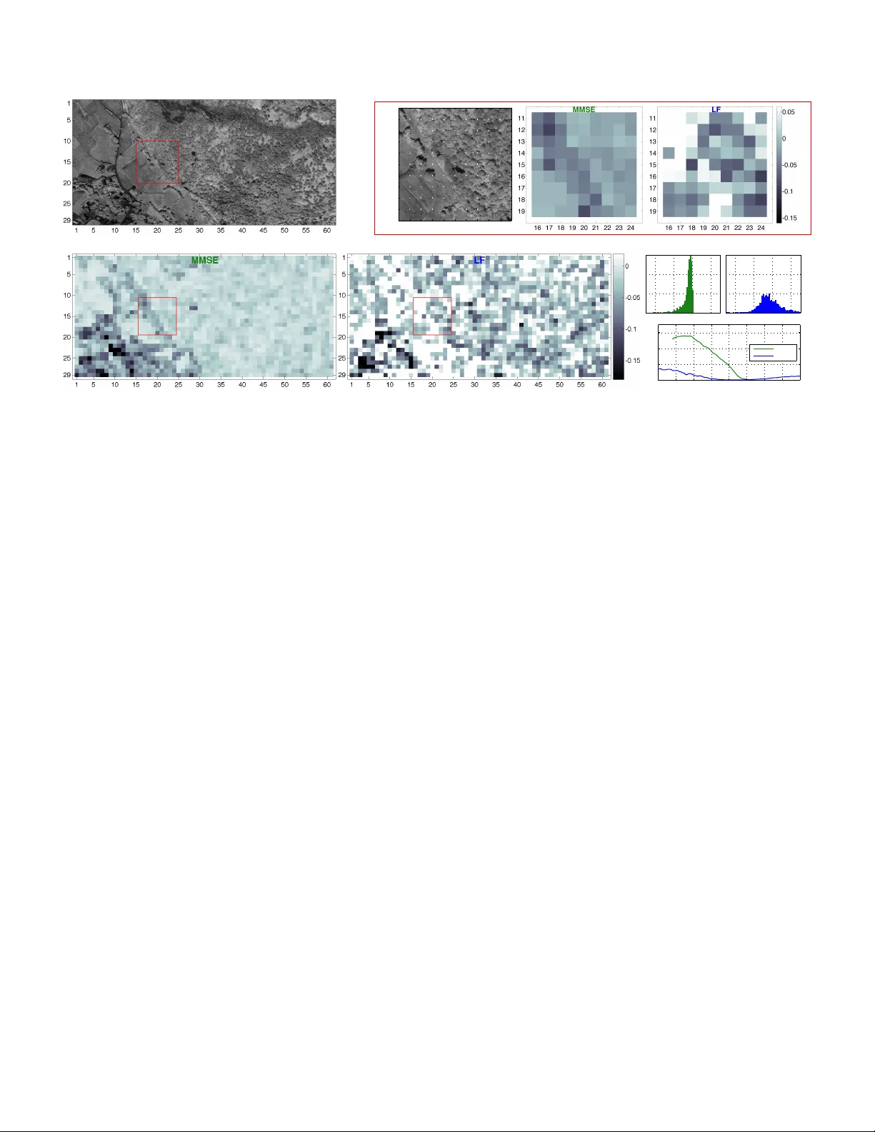
Ba y esian Estimation of the Multifractalit y P arameter for Image T exture Using a Whittle Appro ximation S. Com brexelle, H. W endt ∗ , Memb er, IEEE , N. Dobigeon, Senior Memb er, IEEE , J.-Y. T ourneret, Senior Memb er, IEEE , S. McLaughlin, F el low, IEEE , P . Abry , F el low, IEEE ∗ † ‡§ Abstract T exture c haracterization is a central elemen t in man y image processing applications. Multifractal analysis is a useful signal and image pro cessing to ol, y et, the accurate estimation of multifractal param- eters for image texture remains a c hallenge. This is due in the main to the fact that current estima- tion pro cedures consist of p erforming linear regres- sions across frequency scales of the t wo-dimensional (2D) dyadic w av elet transform, for which only a few suc h scales are computable for images. The strongly non-Gaussian nature of m ultifractal pro cesses, com- bined with their complicated dep endence structure, mak es it difficult to dev elop suitable models for pa- rameter estimation. Here, we propose a Ba yesian pro cedure that addresses the difficulties in the esti- mation of the m ultifractality parameter. The orig- inalit y of the pro cedure is threefold: The construc- tion of a generic semi-parametric statistical mo del for the logarithm of wa v elet leaders; the formula- tion of Ba yesian estimators that are asso ciated with this model and the set of parameter v alues admitted b y m ultifractal theory; the exploitation of a suitable Whittle appro ximation within the Ba y esian mo del whic h enables the otherwise infeasible ev aluation of the p osterior distribution asso ciated with the mo del. P erformance is assessed n umerically for several 2D m ultifractal pro cesses, for several image sizes and a large range of pro cess parameters. The pro ce- dure yields significant b enefits ov er current b ench- mark estimators in terms of estimation p erformance ∗ This work w as supp orted by ANR BLANC 2011 AMA TIS BS0101102 and ANR Pro ject Hypanema ANR-12-BS03-003. S. Com- brexelle w as supported by the Direction G´ en´ erale de l’Armement (DGA). S. McLaughlin ackno wledges the supp ort of EPSRC grant num b er EP/J015180/1. † S. Com brexelle, N. Dobigeon, J.-Y. T ourneret and H. W endt are with IRIT Laboratory , INP-ENSEEIHT, Univ ersity of T oulouse, CNRS, T oulouse, F rance (email: firstname.lastname@enseeih t..fr) ‡ S. McLaughlin is with the School of Engineering and Phys- ical Sciences, Heriot-W att Universit y , Edin burgh, UK (email: s.mclaughlin@hw.ac.uk) § P . Abry is with the Physics Dept., Ecole Normale Sup ´ erieure de Lyon, CNRS, F rance (email: patrice.abry@ens-lyon.fr) and ability to discriminate b etw een the t wo most commonly used classes of m ultifractal pro cess mo d- els. The gains in p erformance are particularly pro- nounced for small image sizes, notably enabling for the first time the analysis of image patches as small as 64 × 64 pixels. Index terms— T exture characterization, Multifractal analysis, W a velet leaders, Bay esian estimation, Whittle ap- pro ximation, Multiplicative cascades, F ractional Brownian motion 1 In tro duction 1.1 Con text and motiv ation Since the early origins of digital image pro cessing, texture has b een recognized as one of the central c haracteristic fea- tures in images. There is no common definition for tex- ture, and different paradigms hav e b een introduced in the literature [24]. Several authors ha ve prop osed to mo del tex- ture using random fractals, scale in v ariance or self-similarity [29, 43]. Indeed, it has b een reported in the literature that scale inv arian t pro cesses are relev an t and effective mo dels for textures asso ciated with a large class of natural images, see, e.g., [16, 59, 63]. The concepts of scale in v ariance and self-similarit y are deeply tied to the degree of p oint wise singular behavior or lo c al r e gularity of the image amplitudes [39, 45]. It has long b een recognized that multiscale and w av elet analyzes consti- tute ideal to ols to study data regularit y [1, 25, 41, 45, 58]. It is therefore not surprising that these tools pla y a cen tral role not only for the study of image con tours (edges), but also for texture c haracterization [18, 37, 51]. Y et, while contours are essen tially isolated singularities, the texture models con- sist of densely interw ov en sets of singularities of different regularit y strength. Multifr actal analysis provides a mathe- matical framew ork for the study of such sp atial fluctuations of lo c al r e gularity and texture characterization is therefore no w adays often conducted using this to ol [7, 31]. Multifractal analysis. The lo cal regularit y of an image X is commonly measured using the so-called H¨ older ex- p onent h ( t ) [25, 45]. Qualitatively , the smaller h ( t 0 ), the rougher X is at spatial lo cation t 0 and the larger h ( t 0 ), the 1 smo other X is at t 0 . The goal of m ultifractal analysis is the estimation of the multifr actal sp e ctrum D ( h ), whic h pro- vides a glob al description of the spatial fluctuations of h ( t ). It is defined as the collection of the fractal dimensions of the sets of p oints for which the H¨ older exp onen t tak es the same v alue [25, 45], cf., Section 2.1. Multifractal analysis has recently matured in to a standard image pro cessing to ol and has been successfully used in a large num b er of appli- cations including texture classification [59, 63], biomedical applications [11, 30], physics [44, 48] and art inv estigation [2, 19, 27, 28]. In most applications, the e stimation of D ( h ) cannot b e based d irectly on its definition [25]. Instead, a so-called mul- tifr actal formalism is constructed based on multiresolution co efficien ts T X ( a, k ), essen tially capturing the con tent of the image X around the discrete spatial location k for a given frequency scale a = 2 j . Examples are giv en b y incremen ts, w a velet coefficients and more recently w a v e let leaders ` ( j, k ) [25] (defined in Section 2.2), which yield the current b ench- mark multifractal formalism. The multifractal formalism pro vides an expansion of the m ultifractal sp ectrum of the image X in terms of the so-called lo g-cumulants c p , p ≥ 1 [26, 58] D ( h ) = 2 + c 2 2!  h − c 1 c 2  2 + − c 3 3!  h − c 1 c 2  3 + − c 4 + 3 c 3 2 /c 2 4!  h − c 1 c 2  4 + . . . (1) when c 2 < 0, while D ( h ) = δ ( h − c 1 ) when c 2 ≡ 0 ( c 2 cannot b e p ositive theoretically [15, 25, 45]). Estimation of c 2 . The leading order co efficients c p pro- vide a relev ant summary of the multifractal prop erties of X in applications where it would often not b e conv enient to handle an entire function D ( h ) [15, 26, 55, 58]. The first log-cum ulan t c 1 , for instance, is the mo de of D ( h ) and can b e read as a measure for the “a v erage” smo othness of X . More imp ortantly , the co efficien t c 2 , referred to as the mul- tifr actality or intermittency parameter, is directly related to the width of D ( h ) and captures the multifractal signature (i.e., the fluctuations of the local regularit y) of the image X . Its primary imp ortance stems from the fact that it enables the iden tification of the tw o ma jor classes of multifractal sto c hastic pro cesses: self-similar pro cesses for which c 2 = 0 and multifractal m ultiplicative cascade (MMC) based pro- cesses for which c 2 is strictly negative [57]. While the former class is tied deeply to additive constructions, the latter is based on multiplicativ e constructions and is hence linked to fundamen tally differen t ph ysical principles [22, 39, 45]. More- o v er, the magnitude of c 2 quan tifies the degree of multi- fractalit y of an image for the latter class. F or an ov erview and details on scale in v ariant and multifractal pro cesses, the reader is referred to, e.g., [33, 45] and references therein. In the seminal con tribution [15], it has b een shown that the log-cum ulants c p are tied to the quantities ` ( j, k ) through the k ey relation Cum p [log ` ( j, k )] = c 0 p + c p log 2 j , where Cum p [ · ] is the p -th order cumulan t. In particular C 2 ( j ) , V ar [log ` ( j, k )] = c 0 2 + c 2 log 2 j . (2) Relation (2) leads to the definition of the current standard and b enchmark estimator for the parameter c 2 , based on linear regression of the sample v ariance, denoted by d V ar, of log ` ( j, k ) o ver a range of scales j ∈ [ j 1 , j 2 ] ˆ c 2 = 1 log 2 j 2 X j = j 1 w j d V ar[log ` ( j, · )] (3) where w j are suitably defined regression weigh ts [55, 58]. Limitations. The use of multifractal analysis remains re- stricted to images of relatively large size (of order 512 2 pix- els) because a sufficient n um b er of scales j m ust b e av ailable to p erform the linear regression (3). While a similar issue is encoun tered for the analysis of 1D signals, it is significantly more severe for images: indeed, mo dulo b order effects of the wa velet transform, the num b er of a v ailable scales is pro- p ortional to the logarithm of the num b er of samples for 1D signals and to the logarithm of the squar e r o ot of the num- b er of pixels for an image. F or instance, for a 1D signal with 256 × 256 = 65536 samples, j 2 = 13 or 14 scales can b e com- puted, while j 2 = 4 or 5 for an image of N × N = 256 × 256 pixels. In addition, the finest scale, j = 1, should not b e used in (3), see, e.g., [53]. The practical consequences for the multifractal analysis of images are severe: First, images of small size and th us image p atches cannot b e analyzed in practice. Second, (3) yields mo dest p erformance for images when compared with 1D signals of equiv alent sample size [58], making it difficult to discriminate b et w een c 2 ≡ 0 and v alues c 2 < 0 that are encoun tered in applications (typically , c 2 lies b etw een − 0 . 01 and − 0 . 08). The goal of this work is to propose and v alidate a no v el pro cedure for the estimation of c 2 for images that addresses these difficulties. 1.2 Related w orks There are a limited n um b er of rep orts in the literature that attempt to ov ercome the limitations of multifractal analy- sis for images describ ed ab ov e. The gener alize d metho d of moments has been proposed and studied in, e.g., [9, 35, 36] and form ulates parameter inference as the solution (in the least squares sense) of an ov er-determined system of equa- tions that are derived from the momen ts of the data. The metho d dep ends strongly on fully parametric mo dels and yields, to the b est of our knowledge, only limited b enefits in practical applications. Although classical in parameter inference, maxim um like- liho od (ML) and Bay esian estimation metho ds hav e mostly b een formulated for a few sp ecific self-similar and m ulti- fractal pro cesses [12, 62]. The main reason for this lies in the complex statistical prop erties of most of these pro cesses, 2 whic h exhibit marginal distributions that are strongly non- Gaussian as w ell as in tricate algebraically decaying dep en- dence structures that remain p o orly studied to date. The same remark is true for their w av elet coefficients and w av elet leaders, see, e.g., [42, 52]. One exception is given by the fractional Bro wnian mo- tion (in 1D) and fractional Brownian fields (in 2D) (fBm), that are jointly Gaussian self-similar (i.e., c 2 ≡ 0) pro cesses with fully parametric co v ariance structure appropriate for ML and Bay esian estimation. Examples of ML and Bay esian estimators for 1D fBm formulated in the sp ectral or w av elet domains can b e found in [12, 17, 40, 62]. F or images, an ML estimator has been prop osed in [34] (note, ho w ever, that the estimation problem is reduced to a univ ariate formulation for the ro ws / columns of the image there). As far as MMC pro cesses are concerned, [32] proposes an ML approach in the time domain for one sp ecific pro- cess. How ever, the metho d relies strongly on the particular construction of this process and cannot easily accommodate more general mo del classes. Moreo ver, the metho d is for- m ulated for 1D signals only . Finally , a Ba y esian estimation pro cedure for the parameter c 2 of multifractal time series has recently b een prop osed in [56]. Unlik e the metho ds men tioned ab o v e, it do es not rely on sp ecific assumptions but instead emplo ys a heuristic semi-parametric mo del for the statistics of the logarithm of wa velet leaders asso ciated with univ ariate MMC pro cesses. Y et, it is designed for and can only be applied to univ ariate time series of small sample size. 1.3 Goals and con tributions The use of fully parametric mo dels for the data can be very restrictiv e in many real-w orld applications. Therefore, the goal and the main contribution of this work is to study a Ba y es ian estimation pro cedure for the multifractalit y pa- rameter c 2 with as few as p ossible assumptions on the data (essen tially , the relation (2)) that can actually be applied to real-w orld images of small as well as large sizes. T o this end, w e adopt a strategy that is inspired b y [56] and develop the k ey elements that are required for its form ulation for images. First, w e sho w b y means of n umerical sim ulations that the distribution of the logarithm of w a v elet leaders log ` ( j, k ) of 2D MMC pro cesses can, at each scale j , b e well ap- pro ximated by a multiv ariate Gaussian distribution. In- spired by the cov ariance prop erties induced by the mul ti- plicativ e nature of cascade constructions, we propose a new generic radial symmetric mo del for the v ariance-cov ariance of this distribution. This second-order statistical mo del is parametrized only by the tw o parameters c 2 and c 0 2 in (2) and enables us to formulate estimation in a Bay esian frame- w ork. Second, we formulate a Ba y esian estimation procedure for the parameter c 2 of images that p ermits to take into accoun t the constraints that are associated with the proposed statis- tical model. T o this end, an appropriate prior distribution is assigned to the parameter v ector ( c 2 , c 0 2 ) which essen tially ensures that the v ariance (2) is p ositive. Additional prior information, if av ailable, can easily b e incorp orated. The Ba y e sian estimators of c 2 asso ciated with the p osterior dis- tribution of in terest cannot b e ev aluated directly b ecause of the constrain ts that the parameter v ector ( c 2 , c 0 2 ) has to satisfy . Therefore, w e design a suitable Mark ov c hain Mon te Carlo (MCMC) algorithm that generates samples that are asymptotically distributed according to the p osterior dis- tribution of interest. These samples are in turn used to appro ximate the Bay esian estimators. More precisely , we prop ose a random-w alk Metrop olis-Hastings sc heme to ex- plore efficiently the posterior distribution according to the admissible set of v alues for c 2 and c 0 2 . Finally , the exact ev aluation of the lik eliho od asso ciated with the proposed mo del for the log-wa v elet leaders requires the computation of the in verse and the determinan t of large dense matrices, which is n umerically and computationally to o demanding for practical applications. T o obtain a sta- ble and efficient algorithm that can actually b e applied to images, follo wing in tuitions developed in the univ ariate case, cf. e.g., [12], we approximate the exact likelihoo d with a Whittle-type expansion that is adapted to the prop osed mo del and can b e efficien tly ev aluated in the sp ectral do- main. The proposed algorithm for the estimation of the m ulti- fractalit y parameter c 2 is effective b oth for small and large image sizes. Its p erformance is asse ssed numerically by means of Monte Carlo sim ulations for t wo classical and rep- resen tativ e 2D MMC constructions, the canonical Mandel- brot cascades (CMC) [39] and comp ound Poisson cascades (CPC) [10], using the most common m ultipliers, and a large range of process parameters and sample sizes from 64 × 64 to 512 × 512 pixels. Complementary results are provided for 2D fBms (that are self-similar but not MMC). Our results indicate that the prop osed estimation pro cedure is robust with resp ect to different choices of process constructions and greatly outp erforms (2), in particular for small images and for iden tifying a v alue c 2 ≡ 0. It enables, for the first time, a m ultifractal analysis of images (or image patc hes) whose sizes are as small as 64 × 64 pixels. The remainder of this work is organized as follows. Sec- tion 2 summarizes the main concepts of m ultifractal analysis and the wa velet leader m ultifractal formalism. Section 3 in- tro duces the statistical mo del and the Ba y esian framew ork underlying the estimation pro cedure for the parameter c 2 of images, which is form ulated in Section 4. Numerical results are given in Section 5. In Section 6, the proposed procedure is applied to the patc h-wise analysis of a real-world image, illustrating its p oten tial b enefits for practical applications. Finally , Section 7 concludes this pap er and presents some future work. 3 2 Multifractal analysis of Images Let X : R 2 → R denote the 2D function (image) to b e analyzed. The image X is assumed to b e lo cally b ounded in what follows (see Section 2.2 for a practical solution to circum v ent this prerequisite). 2.1 Multifractal analysis H¨ older exponent. Multifractal analysis aims at charac- terizing the image X in terms of the fluctuations of its lo c al r e gularity , characterized by the so-called H¨ older exp onent , whic h is defined as follo ws [25, 45]. The image X is said to b elong to C α ( t 0 ) if there exists α > 0 and a p olynomial P t 0 of degree smaller than α suc h that | | X ( t ) − P t 0 ( t ) | | ≤ C | | t − t 0 | | α where | | · | | is the Euclidian norm. The H¨ older exp onent at p osition t 0 is the largest v alue of α suc h that this inequality holds, i.e., h ( t 0 ) , sup { α : X ∈ C α ( t 0 ) } . (4) Multifractal sp ectrum. F or large classes of sto chas- tic pro cesses, the H¨ older exp onents h ( t ) can b e theoreti- cally sho wn to b ehav e in an extremely erratic wa y [25, 26]. Therefore, m ultifractal analysis pro vides a glob al description of the spatial fluctuations of h ( t ) in terms of the multifr ac- tal sp e ctrum D ( h ). It is defined as the Hausdorff dimension (denoted dim H ) of the sets of p oin ts at which the H¨ older exp onen t takes the same v alue, i.e., D ( h ) , dim H  E h = { t : h ( t = h }  . (5) F or more details on multifractal analysis and a precise defi- nition of the Hausdorff dimension, see, e.g., [25, 26]. 2.2 W a v elet leader m ultifractal formalism Historically , multifractal formalisms hav e b een prop osed based on increments or w av elet co efficien ts. These c hoices of multiresolution quantities lead to b oth theoretical and practical limitations, see [55, 58] for a discussion. Recen tly , it has been sho wn that a relev ant m ultifractal formalism can b e constructed from the wavelet le aders [25, 26, 55], which are sp ecifically tailored for this purp ose. W a velet coefficients. W e assume that the image is giv en in form of discrete sample v alues X ( k ), k = ( k 1 , k 2 ). A t w o-dime nsional (2D) orthonormal discrete wa velet trans- form (DWT) can b e obtained as the tensor pro duct of one-dimensional (1D) DWT as follows. Let G 0 ( k ) and G 1 ( k ) denote the low-pass and high-pass filters defining a 1D DWT. These filters are asso ciated with a mother w a velet ψ , characterized by its n um b er of v anishing mo- men ts N ψ > 0. F our 2D filters G ( m ) ( k ), m = 0 , . . . , 3 are defined by tensor pro ducts of G i , i = 1 , 2. The 2D low- pass filter G (0) ( k ) , G 0 ( k 1 ) G 0 ( k 2 ) yields the appro ximation co efficien ts D (0) X ( j, k ), whereas the high-pass filters defined b y G (1) ( k ) , G 0 ( k 1 ) G 1 ( k 2 ), G (2) ( k ) , G 1 ( k 1 ) G 0 ( k 2 ) and G (3) ( k ) , G 1 ( k 1 ) G 1 ( k 2 ) yield the w av elet (detail) co effi- cien ts D ( m ) X ( j, k ), m = 1 , 2 , 3 as follo ws: at the finest scale j = 1, the D ( m ) X ( j, k ), m = 0 , . . . , 3 are obtained b y conv olv- ing the image X with G ( m ) , m = 0 , . . . , 3, and decimation; for the coarser scales j ≥ 2 they are obtained iteratively b y con v olving G ( m ) , m = 0 , . . . , 3, with D (0) X ( j − 1 , · ) and decimation. F or scaling and multifractal analysis purposes, the approximation co efficients D (0) X are discarded and it is common to normalize the wa velet coefficients according to the L 1 -norm d ( m ) X ( j, k ) , 2 − j D ( m ) X ( j, k ) , m = 1 , 2 , 3 (6) so that they repro duce the self-similarity exp onent for self- similar pro cesses [7]. F or a formal definition and details on (2D) wa velet transforms, the reader is referred to [5, 37]. W a velet leaders. Denote as λ j, k = { [ k 1 2 j , ( k 1 + 1)2 j ) , [ k 2 2 j , ( k 2 + 1)2 j ) } the dyadic cub e of side length 2 j cen tered at k 2 j and 3 λ j, k = [ n 1 ,n 2 ∈{− 1 , 0 , 1 } λ j,k 1 + n 1 ,k 2 + n 2 the union of this cub e with its eigh t neigh b ors. The w av elet leaders are defined as the largest wa velet co efficient magni- tude within this neighborho o d o ver all finer scales [25] ` ( j, k ) ≡ ` ( λ j, k ) , sup m ∈ (1 , 2 , 3) ,λ 0 ⊂ 3 λ j, k | d ( m ) X ( λ 0 ) | . (7) W av elet leaders repro duce the H¨ older exp onent as follo ws h ( t 0 ) = lim inf j →−∞  log ` ( λ j, k ( t 0 ))  log 2 j  (8) where λ j, k ( t 0 ) denotes the cub e at scale j including the spa- tial lo cation t 0 [25]. It has b een shown that (8) is the theo- retical k ey prop erty required for constructing a multifractal formalism, see [25] for details. In particular, it can b e sho wn that the wavelet le ader multifr actal formalism (WLMF), i.e., the use of (1) with co efficients c p estimated using wa velet leaders, is v alid for large classes of m ultifractal mo del pro- cesses, see [55, 58] for details and discussions. The WLMF has been extensively studied b oth theoretically and in terms of estimation p erformance and constitutes the b enc hmark to ol for p erforming multifractal analysis, cf. e.g., [55, 58]. Negativ e regularity . The WLMF can be applied to lo cally b ounded images (equiv alently , to images with strictly p ositiv e uniform regularit y) only , see [3, 55, 58] for precise definitions and for pro cedures for assessing this condition in practice. How ever, it has been rep orted that a large n um b er 4 of real-world images do not satisfy this prerequisite [58, 59]. In these cases, a practical solution consists of constructing the WLMF using the mo dified wa velet co efficien ts d ( m ) ,α X ( j, k ) , 2 αj d ( m ) X ( j, k ) , α > 0 (9) instead of d ( m ) X in (7). When α is chosen sufficiently large, the WLMF holds (see [58] for details ab out the theoretical and practical consequences implied by this mo dification). Finally , note that the abov e analysis as well as the WLMF are meaningful for homo gene ous multifr actal functions X , for which the multifractal sp ectra D ( h ) of different subsets of t are identical. This excludes the class of multifr actional mo dels [8, 64], for which the function h ( t ) is given b y a smo oth non-stationary evolution. Such models, also of in- terest in other application con texts, are not considered here, as the focus is on multifractalit y parameter c 2 whic h is not relev an t to c haracterize multifractional processes. 3 Ba y esian framework In this section, a nov el empirical second-order statistical mo del for the logarithm of w av elet leaders for 2D MMC pro- cesses is prop osed. This model is the k ey to ol for estimating the multifractalit y parameter c 2 in a Ba y esian framework. 3.1 Mo deling the statistics of log-wa v elet leaders Marginal distribution mo del. It has recen tly b een ob- serv ed that for 1D signals the distribution of the lo g-wavelet le aders l ( j, k ) , log ` ( j, k ) (10) can b e reasonably well approximated b y a Gaussian distri- bution [56]. Here, we numerically inv estigate the marginal distributions of l ( j, · ) for 2D images. T o this end, a repre- sen tativ e selection of scaling pro cesses (the MMC pro cesses CMC-LN, CMC-LP , CPC-LN and CPC-LP , as w ell as fBm, where LN stands for log-Normal and LP for log-P oisson, re- sp ectiv ely) hav e b een analyzed for a wide range of pro cess parameters (see Section 5.1 for a description of these pro- cesses). Representativ e examples of quantile-quan tile plots of the standard Normal distribution against empirical distri- butions of log-wa velet leaders (scale j = 2) asso ciated with CPC-LN, CPC-LP and fBm are plotted in Fig. 1 (upp er ro w). Clearly , the normal distribution pro vides, within ± 3 standard deviations, a reasonable approximation for the marginal distribution of log-wa velet leaders of images for b oth members of the MMC class. It is also the case for the fBm, a Gaussian self-similar pro cess that is not a member of MMC. Note that the fact that the marginal distributions of the log-wa velet leaders are approximately Gaussian for scale in v arian t processes confirms the intuitions formulated of e s t i m at i on p e r f or m an c e an d c on s t i t u t e s t h e b e n c h m ar k t o ol f or p e r f or m i n g m u l t i f r ac t al an al y s i s , c f . e . g. , [ 55, 58] . Ne gat i v e r e gu l ar i t y . T h e W LM F c an b e ap p l i e d t o l o c al l y b ou n d e d i m age s ( e q u i v al e n t l y , t o i m age s w i t h s t r i c t l y p os i t i v e u n i f or m r e gu l ar i t y ) on l y , s e e [ 3, 55, 58] f or p r e c i s e d e fi n i t i on s an d f or p r o c e d u r e s f or as s e s s i n g t h i s c o n d i t i on i n p r ac t i c e . Ho w e v e r , i t h as b e e n r e p or t e d t h at a l ar ge n u m b e r of r e al - w or l d i m age s d o n ot s at i s f y t h i s p r e r e q u i s i t e [ 58, 59] . I n t h e s e c as e s , a p r ac t i c al s ol u t i on c on s i s t s of c on s t r u c t i n g t h e W LM F u s i n g t h e m o d i fi e d w a v e l e t c o e ffi cien t s d ( m ) , ↵ X ( j, k ) , 2 ↵ j d ( m ) X ( j, k ) , ↵ > 0 ( 9) i n s t e ad of d ( m ) X i n ( 7) . W h e n ↵ i s c h os e n s u ffi c i e n t l y l ar ge , t h e W LM F h ol d s ( s e e [ 58] f or d e t ai l s ab ou t t h e t h e or e t i c al an d p r ac t i c al c on s e q u e n c e s i m p l i e d b y t h i s m o d i fi c at i on ) . F i n al l y , n ot e t h at t h e ab o v e an al y s i s as w e l l as t h e W LM F ar e m e an i n gf u l f or h o m o gen e o u s m u l t i f r a ct a l f u n c t i on s X , f or w h i c h t h e m u l t i f r ac t al s p e c t r a D ( h ) of d i ↵ eren t subset s of t ar e i d e n t i c al . T h i s e x c l u d e s t h e c l as s of m u l t i f r a ct i o n a l m o d e l s [ 8, 64] , f or w h i c h t h e f u n c t i on h ( t ) i s gi v e n b y a s m o ot h n on - s t at i on ar y e v ol u t i on . S u c h m o d e l s , al s o of i n - t e r e s t i n ot h e r ap p l i c at i on c on t e x t s , ar e n ot c on s i d e r e d h e r e , as t h e f o c u s i s on m u l t i f r ac t al i t y p ar am e t e r c 2 w h i c h i s n ot r e l e v an t t o c h ar ac t e r i z e m u l t i f r ac t i on al p r o c e s s e s . 3B a y e s i a n f r a m e w o r k I n t h i s s e c t i on , a n o v e l e m p i r i c al s e c on d - or d e r s t at i s t i c al m o d e l f or t h e l ogar i t h m of w a v e l e t l e ad e r s f or 2D M M C p r o- c e s s e s i s p r op os e d . T h i s m o d e l i s t h e k e y t o ol f or e s t i m at i n g t h e m u l t i f r ac t al i t y p ar am e t e r c 2 i n a B a y e s i an f r am e w or k . 3 . 1 M o de l i ng t he s t a t i s t i cs o f l o g -w a v e l e t l e a de r s M ar gi n al d i s t r i b u t i on m o d e l . I t h as r e c e n t l y b e e n ob - s e r v e d t h at f or 1D s i gn al s t h e d i s t r i b u t i on of t h e l o g- w a vel et l e a d er s l ( j, k ) , l og ` ( j, k ) ( 10) c an b e r e as on ab l y w e l l ap p r o x i m at e d b y a G au s s i an d i s t r i - b u t i on [ 56] . He r e , w e n u m e r i c al l y i n v e s t i gat e t h e m ar gi n al d i s t r i b u t i on s of l ( j, · ) f or 2D i m age s . T o t h i s e n d , a r e p r e - s e n t at i v e s e l e c t i on of s c al i n g p r o c e s s e s ( t h e M M C p r o c e s s e s C M C - LN, C M C - LP , C P C - LN an d C P C - LP , as w e l l as f B m , w h e r e LN s t an d s f or l og- Nor m al an d LP f or l og- P oi s s on , r e - s p e c t i v e l y ) h a v e b e e n an al y z e d f or a w i d e r an ge of p r o c e s s p ar am e t e r s ( s e e S e c t i on 5. 1 f or a d e s c r i p t i on of t h e s e p r o- c e s s e s ) . R e p r e s e n t at i v e e x am p l e s of q u an t i l e - q u an t i l e p l ot s of t h e s t an d ar d Nor m al d i s t r i b u t i on agai n s t e m p i r i c al d i s t r i - b u t i on s of l og- w a v e l e t l e ad e r s ( s c al e j = 2) as s o c i at e d w i t h C P C - LN, C P C - LP an d f B m ar e p l ot t e d i n F i g. 1 ( u p p e r ro w). − 4 − 3 − 2 − 1 0 1 l (2 , k ) − 5 0 5 − 20 − 15 − 10 − 5 0 5 ln | d (3 ) X (2 , k ) | − 4 − 3 − 2 − 1 0 1 2 − 5 0 5 − 20 − 15 − 10 − 5 0 5 − 5 − 4.5 − 4 − 3.5 − 3 − 5 0 5 − 20 − 15 − 10 − 5 0 Stan dard Normal Stan dard Normal Stan dard Normal CP C - LN CP C - LP fBm F i gu r e 1: Q u an t i l e - q u an t i l e p l ot s of t h e e m p i r i c al d i s t r i b u - t i on s of t h e l og- w a v e l e t l e ad e r s l (2 , k ) ( t op ) an d w a v e l e t c o- e ffi c i e n t s l og d (3) X (2 , k ) ( b ot t om ) agai n s t s t an d ar d n or m al f or C P C - LN ( l e f t c ol u m n ) an d C P C - LP ( c e n t e r c ol u m n ) w i t h c 2 =  0 . 04, r e s p e c t i v e l y , an d f or f B m ( r i gh t c ol u m n ) . C l e ar l y , t h e n or m al d i s t r i b u t i on p r o v i d e s , w i t h i n ± 3 s t an d ar d d e v i at i on s , a r e as on ab l e ap p r o x i m at i on f or t h e m ar gi n al d i s t r i b u t i on of l og- w a v e l e t l e ad e r s of i m age s f or b ot h m e m b e r s of t h e M M C c l as s . I t i s al s o t h e c as e f o r t h e f B m , a G au s s i an s e l f - s i m i l ar p r o c e s s t h at i s n ot a m e m b e r of M M C . Not e t h at t h e f ac t t h at t h e m ar gi n al d i s t r i b u t i on s of t h e l og- w a v e l e t l e ad e r s ar e ap p r o x i m at e l y G au s s i an f or s c al e i n v ar i an t p r o c e s s e s c on fi r m s t h e i n t u i t i on s f or m u l at e d b y M an d e l b r ot [ 38] . Ho w e v e r , i t i s n ot a t r i v i al fi n d i n g: T h e r e i s n o a p r i or i r e as on f or t h i s p r op e r t y e v e n i f t h e an al y z e d s t o c h as t i c p r o c e s s h as l og- n or m al m ar gi n al s ( as i s t h e c as e f or C M C - LN, f or i n s t an c e ) . I n d e e d , i t i s not the c as e f or t h e l ogar i t h m of t h e ab s ol u t e v al u e of w a v e l e t c o e f - fi c i e n t s w h os e m ar gi n al d i s t r i b u t i on s ar e s i gn i fi c an t l y m or e c om p l i c at e d an d s t r on gl y d e p ar t f r om G au s s i an , c f . , F i g. 1 ( b ot t om r o w ) . V ar i an c e - c o v ar i an c e m o d e l . We i n t r o d u c e a m o d e l f or t h e c o v ar i an c e of t h e l ogar i t h m of 2D w a v e l e t l e ad - e r s f or M M C p r o c e s s e s at fi x e d s c al e j d e n ot at e d as Co v [ l ( j, k ) ,l ( j, k +  k ) ] . I t i s m ot i v at e d b y t h e as y m p - t ot i c c o v ar i an c e of t h e l ogar i t h m of m u l t i s c al e q u an t i t i e s ge n e r i c al l y as s o c i at e d w i t h m u l t i p l i c at i v e c on s t r u c t i on ( c . f . [ 39] ) , s t u d i e d i n d e t ai l f or w a v e l e t c o e ffi c i e n t s of 1D r an d om w a v e l e t c as c ad e s i n [ 6] , an d al s o b y r e c e n t n u m e r i c al r e s u l t s ob t ai n e d f or t h e c o v ar i an c e of t h e l ogar i t h m of 1D w a v e l e t l e ad e r s f or M M C p r o c e s s e s [ 56] . T h e s e r e s u l t s s u gge s t a l i n e ar d e c a y of C o v [ l ( j, k ) ,l ( j, k +  k ) ] i n l og c o or d i n at e s l og  k , w i t h s l op e gi v e n b y t h e p ar am e t e r c 2 . Nu m e r i c al s i m u l at i on s w i t h 2D M M C p r o c e s s e s f or a w i d e r an ge of p r o- c e s s p ar am e t e r s ( d e t ai l e d i n S e c t i on 5. 1) i n d i c a t e t h at t h e e m p i r i c al i n t r a- s c al e c o v ar i an c e i s r ad i al l y s y m m e t r i c an d d e c a y s as c 2 l og  r wi t h  r , ||  k || f or an i n t e r m e d i ar y 5 Figure 1: Quantile-quan tile plots of the empirical distribu- tions of the log-wa velet leaders l (2 , k ) (top) and w av elet co- efficien ts log d (3) X (2 , k ) (bottom) against standard normal for CPC-LN (left column) and CPC-LP (cen ter column) with c 2 = − 0 . 04, resp ectively , and for fBm (righ t column). 0 0 0 0.05 0.1 0.15 0.2 ∆ k 1 ∆ k 2 Sa m pl e c o va r i a nc e Co v[ l (2 , k ) ,l (2 , k + ∆ k )] (a) Sample co v ariance 0 0 ∆ k 1 ∆ k 2 Mo d e l ρ j ( ∆ r ; θ ) (b) Radial model 0 2 4 6 0 0.1 0.2 0.3 lo g 2 ( ∆ r +1 ) ∆ k 2 = ∆ k 1 Co v j =2 Model j =2 Co v j =3 Model j =3 (c) Slice  k 2 =  k 1 0 2 4 6 lo g 2 ( ∆ r +1 ) ∆ k 2 =0 Co v j =2 Model j =2 Co v j =3 Model j =3 (d) Slice  k 2 =0 F i gu r e 2: F i t t i n g b e t w e e n t h e s am p l e c o v ar i an c e ( a) , a v e r - age d on 100 r e al i z at i on s of C M C - LN ( [ N, c 2 ]= [ 2 9 ,  0 . 04] ) , an d t h e p ar am e t r i c c o v ar i an c e ( b ) ; ( c ) an d ( d ) c om p ar e t h e m o d e l ( b l u e ) an d t h e s am p l e c o v ar i an c e ( r e d ) f or t w o s l i c e s . r an ge of v al u e s  r gi v e n b y 3 <  r   r max j Co v [ l ( j, k ) ,l ( j, k +  k )] ⇡ % (1) j (  r ; c 2 ) ,  + c 2 ( l og 2  r + j ) l og 2 ( 11) where  r max j = p 2( p n j  1) an d n j ⇡b N 2 / 2 2 j c d e n ot e s t h e n u m b e r of w a v e l e t l e ad e r s at s c al e 2 j of an N ⇥ N i m age . T h e c on s t an t  i s f ou n d t o b e w e l l ap p r o x i m at e d b y u s i n g t h e h e u r i s t i c c on d i t i on % (1) j ( b p n j / 4 c ; c 2 ) ) = 0, w h e r e t h e op e r at or bc t r u n c at e s t o i n t e ge r v al u e s . T h e t h e or e t i c al v ar i an c e of t h e l og - w a v e l e t l e ad e r s i s gi v e n by C 2 ( j )= C 2 ( j ; c 2 ,c 0 2 ) d e fi n e d i n ( 2) . F i n al l y , t h e s h or t - t e r m c o v ar i an c e i s m o d e l e d as a l i n e c on n e c t i n g C 2 ( j ; c 2 ,c 0 2 ) at  r = 0 an d % (1) j (  r ; c 2 ) at  r = 3 as f ol l o w s % (0) j (  r ; c 2 ,c 0 2 ) , l og (  r + 1) l og 4 [ % (1) j ( 3; c 2 )  C 2 ( j ; c 2 ,c 0 2 )] + C 2 ( j ; c 2 ,c 0 2 ) . ( 12) C om b i n i n g ( 2) , ( 11) an d ( 12) y i e l d s t h e f ol l o w i n g f u l l m o d e l f or t h e c o v ar i an c e , p ar am e t r i z e d b y t w o p ar am e t e r s ✓ = [ c 2 ,c 0 2 ] T on l y % j (  r ; ✓ )= 8 > < > : C 2 ( j ; c 2 ,c 0 2 )  r =0 % (0) j (  r ; c 2 ,c 0 2 )0   r  3 m ax ( 0 , % (1) j (  r ; c 2 )) 3   r   r max j . ( 13) He r e , on l y t h e p os i t i v e p or t i on s of % (1) j ar e c on s i d e r e d f or n u m e r i c al r e as on s ( c on d i t i on i n g of t h e c o v ar i an c e m at r i x ) . T h e p r op os e d c o v ar i an c e m o d e l i s i l l u s t r at e d i n F i g. 2 f or C M C - LN. T h e j oi n t G au s s i an m o d e l w i t h c o v ar i an c e m o d e l ( 13) as - s u m e s l i m i t e d i n f or m at i on on t h e d e p e n d e n c e b e t w e e n d i ↵ er- e n t s c al e s , e s s e n t i al l y t h e v ar i an c e ( 2) . T h e c or r e s p on d i n g c o v ar i an c e m at r i x m o d e l f or l og- w a v e l e t l e ad e r s at s e v e r al s c al e s j 2 [ j 1 ,j 2 ] h as t h u s b l o c k - d i agon al s t r u c t u r e . F or c on v e n i e n c e an d w i t h ou t l os s of ge n e r al i t y , t h e f or m u l at i on s gi v e n b e l o w an d i n S e c t i on 4 w i l l b e s t at e d i n b l o c k - d i agon al f or m y e t c ou l d b e e x t e n d e d w i t h ou t d i ffi c u l t y t o an y ot h e r v al i d c o v ar i an c e m at r i x m o d e l . 3 . 2 L i k e l i ho o d, pr i o r a nd p o s t e r i o r di s t r i - but i o ns W e f o c u s on t h e e s t i m at i on of t h e p ar am e t e r c 2 an d t h e r e f or e w or k w i t h c e n t e r e d l og- w a v e l e t l e ad e r s b e l o w . Le t l j d e n ot e t h e v e c t or of t h e n j cen t ered co e ffi ci en ts l ( j, k )  b E [ l X ( j, . )] at s c al e j 2 [ j 1 ,j 2 ] , or gan i z e d i n l e x i c ogr ap h i c or d e r , w h e r e b E [ · ] s t an d s f or t h e s am p l e m e an . Le t ⌃ j ( ✓ ) d e n ot e t h e c or r e s p on d i n g n j ⇥ n j c o v ar i an c e m at r i x w h os e e n t r i e s ar e gi v e n b y t h e 2D p ar am e t r i c c o v ar i an c e f u n c t i on m o d e l ( 13) . F or c on v e n i e n c e of n ot at i on , al l c o e ffi c i e n t s ar e s t ac k e d i n a u n i q u e z e r o- m e an v e c t or L =[ l T j 1 ,. . . , l T j 2 ] T . Lik e liho o d. W i t h t h e ab o v e n ot at i on an d as s u m p t i on s , t h e l i k e l i h o o d of l j i s gi v e n b y p ( l j | ✓ ) , exp ⇣  1 2 l T j ⌃ j ( ✓ )  1 l j ⌘ p (2 ⇡ ) n j det ⌃ j ( ✓ ) . ( 14) Us i n g t h e i n d e p e n d e n c e b e t w e e n l ( j, k ) an d l ( j 0 , k 0 ) f or j 6 = j 0 , t h e l i k e l i h o o d of L i s gi v e n b y p ( L| ✓ )= j 2 Y j = j 1 p ( l j | ✓ ) . ( 15) P r i or d i s t r i b u t i on . T h e p ar am e t e r v e c t or ✓ m u s t b e c h o- s e n s u c h t h at t h e v ar i an c e s of l ( j, k ) ar e p os i t i v e , C 2 ( j )  0. W e d e fi n e t h e ad m i s s i b l e s e t A =( A + [ A  ) \ A m ( 16) where A  = { ( c 2 ,c 0 2 ) 2 R 2 | c 2 < 0 an d c 0 2 + c 2 j 2 ln 2 > 0 } , A + = { ( c 2 ,c 0 2 ) 2 R 2 | c 2 > 0 an d c 0 2 + c 2 j 1 ln 2 > 0 } , A m = { ( c 2 ,c 0 2 ) 2 R 2 || c 0 2 | 0 } , A + = { ( c 2 , c 0 2 ) ∈ R 2 | c 2 > 0 and c 0 2 + c 2 j 1 ln 2 > 0 } , A m = { ( c 2 , c 0 2 ) ∈ R 2 | | c 0 2 | < c 0 ,m 2 , | c 2 | < c m 2 } and c m 2 , c 0 ,m 2 quan tify the largest admissible v alues for c 2 and c 0 2 , parameters that need to b e tuned b y practitioners and ma y dep end on the application considered. When no addi- tional prior information is av ailable regarding θ , a uniform prior distribution on the set A is assigned to θ π ( θ ) = U A ( θ ) ∝ 1 A ( θ ) . (17) P osterior distribution and Bay esian estimators. The posterior distribution of θ is obtained from the Ba yes rule p ( θ |L ) ∝ p ( L| θ ) π ( θ ) (18) and can b e used to define the Bay esian maximum a p os- teriori (MAP) and minim um mean squared error (MMSE) estimators given in (20) and (21) b elow. 6 4 Estimation pro cedure The computation of the Bay esian estimators is not straight- forw ard b ecause of the complicated dep endence of the p os- terior distribution (18) on the parameters θ . Sp ecifically , the inv erse and determinant of Σ j in the expression of the lik eliho od (14) do not hav e a parametric form and hence (18) can not b e optimized with resp ect to the parameters θ . In suc h situations, it is common to use a Marko v Chain Mon te Carlo (MCMC) algorithm generating samples that are distributed according to p ( θ |L ). These samples are used in turn to approximate the Bay esian estimators. 4.1 Gibbs sampler The following Gibbs sampler enables the generation of sam- ples { θ ( t ) } N mc 1 that are distributed according to the p os- terior distribution (18). This sampler consists of succes- siv ely sampling according to the conditional distributions p ( c 2 | c 0 2 , L ) and p ( c 0 2 | c 2 , L ) asso ciated with p ( θ |L ). T o gener- ate the samples according to the conditional distributions, a Metrop olis-within-Gibbs pro cedure is used. The instru- men tal distributions for the random walks are Gaussian and ha v e v ariances σ 2 c 2 and σ 2 c 0 2 , resp ectiv ely , whic h are adjusted to ensure an acceptance rate b et ween 0 . 4 and 0 . 6 (to ensure go o d mixing prop erties). F or details on MCMC metho ds, the reader is referred to, e.g., [46]. Sampling according to p ( c 2 | c 0 2 , L ) . At iteration t , de- note as θ ( t ) = [ c ( t ) 2 , c 0 , ( t ) 2 ] T the current state vector. A candidate c ( ? ) 2 is drawn according to the prop osal distri- bution p 1 ( c ( ? ) 2 | c ( t ) 2 ) = N ( c ( t ) 2 , σ 2 c 2 ). The candidate state v ector θ ( ? ) = [ c ( ? ) 2 , c 0 , ( t ) 2 ] T is accepted with probability π c 2 = min(1 , r c 2 ) (i.e., θ ( t + 1 2 ) = θ ( ? ) ) and rejected with probabilit y 1 − π c 2 (i.e., θ ( t + 1 2 ) = θ ( t ) ). Here, r c 2 is the Metrop olis-Hastings acceptance ratio, given by r c 2 = p ( θ ( ? ) |L ) p 1 ( c ( t ) 2 | c ( ? ) 2 ) p ( θ ( t ) |L ) p 1 ( c ( ? ) 2 | c ( t ) 2 ) = 1 A ( θ ( ? ) ) j 2 Y j = j 1 s det Σ j ( θ ( t ) ) det Σ j ( θ ( ? ) ) × exp  − 1 2 l T j  Σ j ( θ ( ? ) ) − 1 − Σ j ( θ ( t ) ) − 1  l j  . (19) Sampling according to p ( c 0 2 | c 2 , L ) . Similarly , at itera- tion t + 1 2 , a candidate c 0 , ( ? ) 2 is prop osed according to the in- strumen tal distribution p 2 ( c 0 , ( ? ) 2 | c 0 , ( t ) 2 ) = N ( c 0 , ( t ) 2 , σ 2 c 0 2 ). The candidate state v ector θ ( ? ) = [ c ( t + 1 2 ) 2 , c 0 , ( ? ) 2 ] T is accepted with probabilit y π c 0 2 = min(1 , r c 0 2 ) (i.e., θ ( t +1) = θ ( ? ) ) and rejected with probability 1 − π c 0 2 (i.e., θ ( t +1) = θ ( t + 1 2 ) ). The Metrop olis-Hastings acceptance ratio r c 0 2 is given by (19) with p 1 replaced by p 2 , c 2 replaced by c 0 2 and t replaced by t + 1 2 . Appro ximation of the Ba yesian estimators. After a burn-in p erio d defined by t = 1 , . . . , N bi , the prop osed Gibbs sampler generates samples { θ ( t ) } N mc t = N bi +1 that are dis- tributed according to the posterior distribution (18). These samples are used to approximate the MAP and MMSE es- timators ˆ θ MMSE , E [ θ |L ] ≈ 1 N mc − N bi N mc X t = N bi +1 θ ( t ) (20) ˆ θ MAP , argmax θ p ( θ |L ) ≈ argmax t>N bi p ( θ ( t ) |L ) . (21) 4.2 Whittle appro ximation The Gibbs sampler defined in subsection 4.1 requires the in- v ersion of the n j × n j matrices Σ j ( θ ) in (19) for each sam- pling step in order to obtain r c 2 and r c 0 2 . These inv ersion steps are computationally prohibitive ev en for very mo dest image sizes (for instance, a 64 × 64 image would require the in v ersion of a dense matrix of size ∼ 1000 × 1000 at scale j = 1 at each sampling step). In addition, it is numerically instable for larger images (due to growing condition n um- b er). T o alleviate this difficulty , we prop ose to replace the exact lik eliho o d (15) with an asymptotic approximation due to Whittle [60, 61]. With the ab ov e assumptions, the col- lection of log-leaders { l ( j, · ) } are realizations of a Gaussian random field on a regular lattice P j = { 1 , .., m j } 2 , where m j = √ n j . Up to an additive constant, the Whittle appro xi- mation for the negativ e logarithm of the Gaussian lik eliho o d (14) reads [4, 12, 23, 61] − log p ( l j | θ ) ≈ p W ( l j | θ ) = 1 2 X ω ∈ D j log φ j ( ω ; θ ) + I j ( ω ) n j φ j ( ω ; θ ) (22) where the summation is taken ov er the spectral grid D j = { 2 π m j b ( − m j − 1) / 2 c , − 1 , 1 , m j − b m j / 2 c} 2 . Here I j ( ω ) is the 2D standard p erio dogram of { l ( j, k ) } k ∈ P j I j ( ω ) =     X k ∈ P j l ( j, k ) exp( − i k T ω )     2 (23) and φ j ( ω ; θ ) is the sp ectral density asso ciated with the co- v ariance function % j (∆ r ; θ ), resp ectively . Without a closed- form expression for φ j ( ω ; θ ), it can be ev aluated n umerically b y discrete F ourier transform (DFT) φ j ( ω ; θ ) =     X k ∈ P j % j ( q k 2 1 + k 2 2 ; θ ) exp( − i k T ω )     . (24) F requency range. It is commonly reported in the liter- ature that the range of frequencies used in (22) can be re- stricted. This is notably the case for the p erio dogram-based estimation of the memory co efficient of long-range dep en- den t time series for which only the low frequencies can b e 7 0 0 − 10 − 5 0 ω 1 ω 2 Pe ri o dog r a m ln I j ( ω ) (a) Periodogram 0 0 − 10 − 5 0 ω 1 ω 2 Mo d e l ln φ j ( ω ; θ ) (b) Parametric sp ectral density 0  /2   10  5 0 ω 1 j =2 ω 2 = ω 1 ln I j ( ω ) ln φ j ( ω ; θ ) (c) Slice ! 2 = ! 1 0  /2   10  5 0 ω 1 j =2 ω 2 =0 ln I j ( ω ) ln φ j ( ω ; θ ) (d) Slice ! 2 =0 F i gu r e 3: F i t t i n g b e t w e e n t h e p e r i o d ogr am ( a) , a v e r age d on 100 r e al i z at i on s of C M C - LN ( [ N, c 2 ,j ]= [ 2 9 ,  0 . 04 , 2] ) , an d t h e m o d e l  j ( ! ; ✓ ) , ob t ai n e d f r om a D F T of % j (  r ; ✓ ). ( c ) an d ( d ) c om p ar e t h e m o d e l ( b l u e ) an d t h e p e r i o d ogr am ( r e d ) f or t w o s l i c e s . b y d i s c r e t e F ou r i e r t r an s f or m ( D F T )  j ( ! ; ✓ )=     X k 2 P j % j ( q k 2 1 + k 2 2 ; ✓ )e x p (  i k T ! )     . ( 24) F r e q u e n c y r an ge . I t i s c om m on l y r e p or t e d i n t h e l i t e r - at u r e t h at t h e r an ge of f r e q u e n c i e s u s e d i n ( 22) c an b e r e - s t r i c t e d . T h i s i s n ot ab l y t h e c as e f or t h e p e r i o d ogr am - b as e d e s t i m at i on of t h e m e m or y c o e ffi c i e n t of l on g- r an ge d e p e n - d e n t t i m e s e r i e s f or w h i c h on l y t h e l o w f r e q u e n c i e s c an b e u s e d , s e e , e . g. , [ 12, 47, 54] . S i m i l ar l y , i n t h e p r e s e n t c on t e x t , t h e p r op os e d s p e c t r al d e n s i t y m o d e l  j ( ! ; ✓ ) y i e l d s an e x c e l - l e n t fi t at l o w f r e q u e n c i e s an d d e gr ad e s at h i gh e r f r e q u e n c i e s . T h i s i s i l l u s t r at e d i n F i g. 3 w h e r e t h e a v e r age p e r i o d ogr am s of l ( j, k ) f or C P C - LN ar e p l ot t e d t oge t h e r w i t h t h e m o d e l  j ( ! ; ✓ ) . W e t h e r e f or e r e s t r i c t t h e s u m m at i on i n ( 22) t o lo w frequencies D † j ( ⌘ )= n ! 2 D j | k ! k 2  p ⌘ 2 ⇡ m j b m j / 2 c o w h e r e t h e fi x e d p ar am e t e r ⌘ ap p r o x i m at e l y c or r e s p on d s t o t h e f r ac t i on of t h e s p e c t r al gr i d D j t h at i s ac t u al l y u s e d . W e d e n ot e t h e ap p r o x i m at i on of p W ( l j | ✓ ) ob t ai n e d b y r e p l ac i n g D j wi t h D † j i n ( 22) b y p † W ( l j | ✓ ) . T h e fi n al W h i t t l e ap p r o x - i m at i on of t h e l i k e l i h o o d ( 15) i s t h e n gi v e n b y t h e f ol l o w i n g 0 0 .2 0 .4 0 . 6 0 . 8 1 − 0.01 0 0.01 0.02 0.03 0.04 0.05 N =2 9 0 0 .2 0 .4 0 . 6 0 . 8 1 c 2 = − 0 . 02 c 2 = − 0 . 08 0 0 .2 0 .4 0 . 6 0 . 8 1 − 0.01 0 0.01 0.02 0.03 0.04 0.05 N =2 8 ηη η m- c 2 s rm s F i gu r e 4: I n fl u e n c e of t h e b an d w i d t h p ar am e t e r , ⌘ , on e s t i - m at i on p e r f or m an c e f or t w o d i ↵ e r e n t s i z e s of LN- C M C an d tw o d i ↵ e r e n t v al u e s of c 2 v al u e s (  0 . 02 i n r e d an d  0 . 08 i n blue). e q u at i on p ( L| ✓ ) ⇡ exp 0 @  j 2 X j = j 1 p † W ( l j | ✓ ) 1 A =e x p 0 B @  j 2 X j = j 1 1 2 X ! 2 D † j ( ⌘ ) l og  j ( ! ; ✓ )+ I j ( ! ) n j  j ( ! ; ✓ ) 1 C A ( 25) u p t o a m u l t i p l i c at i v e c on s t an t . I t i s i m p or t an t t o n ot e t h at t h e r e s t r i c t i on t o l o w f r e q u e n c i e s i n ( 25) i s n ot a r e s t r i c t i on t o a l i m i t e d f r e q u e n c y c on t e n t of t h e i m age ( i n d e e d , s c al e s j 2 [ j 1 ,j 2 ] ar e u s e d ) b u t on l y c on c e r n s t h e n u m e r i c al e v al u - at i on s of t h e l i k e l i h o o d ( 15) . 5 N um e r i ca l e x p e r i m e n t s T h e p r op os e d al gor i t h m i s n u m e r i c al l y v al i d at e d f or s e v e r al t y p e s of s c al e i n v ar i an t an d m u l t i f r ac t al s t o c h as t i c p r o c e s s e s f or d i ↵ e r e n t s am p l e s i z e s an d a l ar ge r an ge of v al u e s f or c 2 . 5 . 1 St o c ha s t i c m ul t i f r a ct a l m o de l pr o ce s s e s C an on i c al M an d e l b r ot C as c ad e ( C M C ) . C M C s [ 39] ar e t h e h i s t or i c al ar c h e t y p e s of m u l t i f r ac t al m e as u r e s . T h e i r c on s t r u c t i on i s b as e d on an i t e r at i v e s p l i t - an d - m u l t i p l y p r o- c e d u r e on an i n t e r v al ; w e u s e a 2D b i n ar y c as c ad e f or t w o di ↵ e r e n t m u l t i p l i e r s : F i r s t , l og- n or m al m u l t i p l i e r s W = 2  U ,w h e r e U ⇠ N ( m, 2 m/ l og 2) i s a G au s s i an r an d om v ar i ab l e ( C M C - LN) ; S e c on d , l og- P oi s s on m u l t i p l i e r s W = 2  e x p ( l og (  ) ⇡  ), w he re ⇡  i s a P oi s s on r an d om v ar i ab l e w i t h p ar am e t e r  =   log 2 (   1) ( C M C - LP ) . F or C M C - LN, t h e l og- c u m u l an t s ar e gi v e n b y c 1 = m + ↵ , c 2 =  2 m an d c p = 0 f or al l p  3. F or C M C - LP , c 1 = ↵ +  ⇣ log (  )   1  1 ⌘ an d al l h i gh e r - or d e r l og- c u m u l an t s ar e n on - z e r o w i t h c p = 8 Figure 3: Fitting b etw een the p erio dogram (a), av eraged on 100 realizations of CMC-LN ([ N , c 2 , j ] = [2 9 , − 0 . 04 , 2]), and the mo del φ j ( ω ; θ ), obtained from a DFT of % j (∆ r ; θ ). (c) and (d) compare the mo del (blue) and the p erio dogram (red) for t w o slices. used, see, e.g., [12, 47, 54]. Similarly , in the present context, the prop osed sp ectral density mo del φ j ( ω ; θ ) yields an excel- len t fit at low frequencies and degrades at higher frequencies. This is illustrated in Fig. 3 where the av erage p erio dograms of l ( j, k ) for CPC-LN are plotted together with the mo del φ j ( ω ; θ ). W e therefore restrict the summation in (22) to lo w frequencies D † j ( η ) = n ω ∈ D j |k ω k 2 ≤ √ η 2 π m j b m j / 2 c o where the fixed parameter η approximately corresp onds to the fraction of the sp ectral grid D j that is actually used. W e denote the appro ximation of p W ( l j | θ ) obtained b y replacing D j with D † j in (22) by p † W ( l j | θ ). The final Whittle appro x- imation of the likelihoo d (15) is then given b y the following equation p ( L| θ ) ≈ exp   − j 2 X j = j 1 p † W ( l j | θ )   = exp    − j 2 X j = j 1 1 2 X ω ∈ D † j ( η ) log φ j ( ω ; θ ) + I j ( ω ) n j φ j ( ω ; θ )    (25) up to a multiplicativ e constant. It is imp ortan t to note that the restriction to lo w frequencies in (25) is not a restriction to a limited frequency conten t of the image (indeed, scales j ∈ [ j 1 , j 2 ] are used) but only concerns the numerical ev alu- ations of the likelihoo d (15). 0 0 .2 0 .4 0 . 6 0 . 8 1 − 0.01 0 0.01 0.02 0.03 0.04 0.05 N =2 9 0 0 .2 0 .4 0 . 6 0 . 8 1 c 2 = − 0 . 02 c 2 = − 0 . 08 0 0 .2 0 .4 0 . 6 0 . 8 1 − 0.01 0 0.01 0.02 0.03 0.04 0.05 N =2 8 ηη η m- c 2 s rm s Figure 4: Influence of the bandwidth parameter, η , on esti- mation p erformance for tw o different sizes of LN-CMC and t w o different v alues of c 2 v alues ( − 0 . 02 in red and − 0 . 08 in blue). 5 Numerical exp eriments The prop osed algorithm is n umerically v alidated for sev eral t yp es of scale in v arian t and m ultifractal sto c hastic processes for different sample sizes and a large range of v alues for c 2 . 5.1 Sto c hastic m ultifractal mo del pro cesses Canonical Mandelbrot Cascade (CMC). CMCs [39] are the historical arc hetypes of m ultifractal measures. Their construction is based on an iterative split-and-multiply pro- cedure on an in terv al; we use a 2D binary cascade for tw o differen t m ultipliers: First, log-normal multipliers W = 2 − U , where U ∼ N ( m, 2 m/ log 2) is a Gaussian random v ariable (CMC-LN); Second, log-Poisson multipliers W = 2 γ exp (log ( β ) π λ ), where π λ is a Poisson random v ariable with parameter λ = − γ log 2 ( β − 1) (CMC-LP). F or CMC-LN, the log-cum ulan ts are given by c 1 = m + α , c 2 = − 2 m and c p = 0 for all p ≥ 3. F or CMC-LP , c 1 = α + γ  log( β ) β − 1 − 1  and all higher-order log-cumulan ts are non-zero with c p = − γ β − 1 ( − log ( β )) p , p ≥ 2. Below, γ = 1 . 05 and β is v aried according to the v alue of c 2 . Comp ound Poisson Cascade (CPC). CPCs w ere in- tro duced to ov ercome certain limitations of the CMCs that are caused by their discrete split-and-multiply construc- tion [10, 16]. In the construction of CPCs, the lo caliza- tion of the multipliers in the space-scale volume follows a P oisson random pro cess with sp ecific prescrib ed density . W e use CPCs with log-normal m ultipliers W = exp( Y ), where Y ∼ N ( µ, σ ) is a Gaussian random v ariable (CPC- LN), or log-P oisson CPCs for which multipliers W are re- duced to a constant w (CPC-LP). The first log-cum ulants of CPC-LN are given by c 1 = −  µ + 1 − exp  µ + σ 2 / 2  + α , c 2 = − ( µ 2 + σ 2 ), and c p 6 = 0 for p ≥ 3. Here, we fix µ = − 0 . 1. F or CPC-LP , c 2 = − log ( w ) 2 . F ractional Bro wnian motion (fBm). W e use 2D fBms as defined in [50]. FBm is not a CMC pro cess and is based 8 T able 1: Estimation p erformance for CMC-LN (a), CPC-LN (b) CMC-LP (c), CPC-LP (d) for sample sizes N = { 2 8 , 2 9 } and j 1 = 2, j 2 = { 4 , 5 } . Best results are marked in b old. (a) CMC-LN c 2 − 0 . 01 − 0 . 02 − 0 . 04 − 0 . 06 − 0 . 08 N = 2 8 m LF − 0 . 015 − 0 . 027 − 0 . 053 − 0 . 066 − 0 . 087 MMSE − 0 . 014 − 0 . 023 − 0 . 042 − 0 . 060 − 0 . 078 s LF 0 . 010 0 . 011 0 . 015 0 . 018 0 . 030 MMSE 0 . 005 0 . 006 0 . 013 0 . 014 0 . 020 rms LF 0 . 011 0 . 014 0 . 019 0 . 019 0 . 030 MMSE 0 . 007 0 . 007 0 . 013 0 . 014 0 . 020 N = 2 9 m LF − 0 . 016 − 0 . 027 − 0 . 049 − 0 . 070 − 0 . 087 MMSE − 0 . 014 − 0 . 025 − 0 . 047 − 0 . 067 − 0 . 087 s LF 0 . 005 0 . 006 0 . 008 0 . 011 0 . 016 MMSE 0 . 002 0 . 004 0 . 006 0 . 008 0 . 012 rms LF 0 . 008 0 . 010 0 . 012 0 . 015 0 . 018 MMSE 0 . 005 0 . 007 0 . 009 0 . 011 0 . 014 (b) CPC-LN c 2 − 0 . 01 − 0 . 02 − 0 . 04 − 0 . 06 − 0 . 08 N = 2 8 m LF − 0 . 013 − 0 . 025 − 0 . 049 − 0 . 066 − 0 . 089 MMSE − 0 . 007 − 0 . 013 − 0 . 035 − 0 . 054 − 0 . 074 s LF 0 . 009 0 . 011 0 . 017 0 . 024 0 . 029 MMSE 0 . 003 0 . 005 0 . 011 0 . 016 0 . 022 rms LF 0 . 010 0 . 012 0 . 020 0 . 025 0 . 031 MMSE 0 . 004 0 . 008 0 . 012 0 . 018 0 . 023 N = 2 9 m LF − 0 . 013 − 0 . 025 − 0 . 045 − 0 . 066 − 0 . 089 MMSE − 0 . 008 − 0 . 015 − 0 . 035 − 0 . 057 − 0 . 079 s LF 0 . 004 0 . 005 0 . 010 0 . 014 0 . 015 MMSE 0 . 002 0 . 003 0 . 006 0 . 009 0 . 013 rms LF 0 . 005 0 . 007 0 . 011 0 . 015 0 . 017 MMSE 0 . 003 0 . 005 0 . 008 0 . 009 0 . 013 (c) CMC-LP (d) CPC-LP c 2 − 0 . 02 − 0 . 04 − 0 . 08 − 0 . 02 − 0 . 04 − 0 . 08 N = 2 8 m LF − 0 . 019 − 0 . 038 − 0 . 076 − 0 . 043 − 0 . 065 − 0 . 120 MMSE − 0 . 017 − 0 . 032 − 0 . 063 − 0 . 029 − 0 . 055 − 0 . 100 s LF 0 . 010 0 . 014 0 . 023 0 . 016 0 . 035 0 . 035 MMSE 0 . 005 0 . 009 0 . 016 0 . 010 0 . 012 0 . 027 rms LF 0 . 010 0 . 014 0 . 023 0 . 028 0 . 043 0 . 050 MMSE 0 . 006 0 . 012 0 . 023 0 . 013 0 . 020 0 . 036 N = 2 9 m LF − 0 . 020 − 0 . 040 − 0 . 075 − 0 . 037 − 0 . 063 − 0 . 100 MMSE − 0 . 019 − 0 . 036 − 0 . 070 − 0 . 031 − 0 . 060 − 0 . 120 s LF 0 . 006 0 . 009 0 . 014 0 . 010 0 . 014 0 . 020 MMSE 0 . 004 0 . 006 0 . 010 0 . 004 0 . 007 0 . 013 rms LF 0 . 006 0 . 009 0 . 015 0 . 020 0 . 027 0 . 032 MMSE 0 . 004 0 . 007 0 . 015 0 . 012 0 . 021 0 . 038 on an additiv e construction instead. Its multifractal and statistical properties are en tirely determined b y a single pa- rameter H such that c 1 = H , c 2 = 0 and c p = 0 for all p > 2, and b elow we set H = 0 . 7. 5.2 Numerical sim ulations W a velet transform. A Daub echies’s mother wa velet with N ψ = 2 v anishing moments is used, and α = 1 in (9), which is sufficient to ensure p ositive uniform regularity for all pro cesses considered. Estimation. The linear regression weigh ts w j in the stan- dard estimator (3) hav e to satisfy the usual constraints P j 2 j 1 j w j = 1 and P j 2 j 1 w j = 0 and can be c hosen to reflect the confidence granted to each d V ar n j [log ` ( j, · )], see [55, 58]. Here, they are chosen prop ortional to n j as suggested in [55]. The linear regression based standard estimator (3) will b e denoted LF (for “linear fit”) in what follows. The Gibbs sampler is run with N mc = 7000 iterations and a burn-in pe- rio d of N bi = 3000 samples. The bandwidth parameter η in (25) has b een set to η = 0 . 3 following preliminary n umerical sim ulations; these are illustrated in Fig. 4 where estima- tion p erformance is plotted as a function of η for LN-CMC ( N = 2 8 top, N = 2 9 b ottom) with tw o differen t v alues of c 2 ( − 0 . 02 in red, − 0 . 08 in blue). As exp ected, η tunes a classical bias-v ariance tradeoff: a large v alue of η leads to a large bias and small standard deviation and vice v ersa. The c hoice η = 0 . 3 yields a robust practical compromise. P erformance assessment. W e apply the LF estimator (3) and the proposed MAP and MMSE estimators (20) and (21) to R = 100 indep endent realizations of size N × N eac h for the ab ov e describ ed multifractal pro cesses. A range of weak to strong multifractalit y parameter v alues c 2 ∈ {− 0 . 01 , − 0 . 02 , − 0 . 04 , − 0 . 06 , − 0 . 08 } and sample sizes N ∈ { 2 6 , 2 7 , 2 8 , 2 9 } are used. The coarsest scale j 2 used for estimation is set suc h that n j 2 ≥ 100 (i.e., the coarsest a v ailable scale is discarded), yielding j 2 = { 2 , 3 , 4 , 5 } , re- sp ectiv ely , for the considered sample sizes. The finest scale j 1 is commonly set to j 1 = 2 in order to a void p ollution from improp er initialization of the wa velet transform, see [53] for details. Performance is ev aluated using the sample mean, the sample standard deviation and the ro ot mean squared error (RMSE) of the estimates av eraged across realizations m = b E [ˆ c 2 ] , s = q d V ar[ ˆ c 2 ] , rms = p ( m − c 2 ) 2 + s 2 . 5.3 Results Estimation p erformance. T ab. 1 summarizes the esti- mation p erformance of LF and MMSE estimators for CMC- LN, CPC-LN, CMC-LP , CPC-LP (subtables (a)-(d), respec- tiv ely) and for sample sizes N = { 2 8 , 2 9 } . The p erformance of the MAP estimator w as found to be similar to the MMSE estimator and therefore is not repro duced here due to space constrain ts. Note, how ever, that different (application de- p enden t) priors for θ may lead to differen t results (here, the non-informativ e prior (17) is used). First, it is observed that the prop osed algorithm sligh tly but systematically outp erforms LF in terms of bias. This 9 (a) 16 17 18 19 20 21 22 23 24 11 12 13 14 15 16 17 18 19 (b) (c) (d) − 0.2 − 0.1 0 0.1 histogram MMSE c 2 − 0.2 − 0.1 0 0.1 histogram LF c 2 − 0.25 − 0.2 − 0.15 − 0.1 − 0.05 0 0.05 0.1 0 0.01 0.02 0.03 c 2 threshold Fisher linear discriminant criterion MMSE LF (e) F i gu r e 5: B an d # 20 of a h y p e r s p e c t r al d at ac u b e ( a) ; e s t i m at e s of c 2 f or o v e r l ap p i n g 64 ⇥ 64 p i x e l p at c h e s ob t ai n e d b y M M S E ( c ) an d LF ( d ) ; z o om s on t h e p at c h e s i n d i c at e d b y a r e d f r am e ( b ) ; t h e c e n t e r s of t h e i m age p at c h e s ar e i n d i c at e d b y w h i t e d ot s i n t h e or i gi n al i m age , t h e d i s t an c e b e t w e e n t w o of t h e d ot s c or r e s p on d s t o on e h al f of t h e p at c h s i z e , ax i s l ab e l s i n d i c at e p at c h n u m b e r s . Hi s t ogr am s an d F i s h e r l i n e ar d i s c r i m i n an t c r i t e r i a f or e s t i m at e s of c 2 ob t ai n e d b y M M S E an d LF ( e ) . c om p u t at i on al c os t , w i t h c om p u t at i on t i m e s of t h e or d e r of 8s ( N = 64) t o 50s ( N = 512) p e r i m age , r e s p e c t i v e l y , on a s t an d ar d d e s k t op c om p u t e r , w h i c h i s t w o or d e r s of m agn i - t u d e l ar ge r t h an t h e c om p u t at i on al c os t of t h e LF e s t i m at or . P e r f or m an c e f or f r ac t i on al B r o w n i an m ot i on . Self- s i m i l ar f B m s w i t h c 2 = 0 d o n ot b e l on g t o t h e c l as s of M M C p r o c e s s e s f or w h i c h t h e p r op os e d e s t i m at i on p r o c e d u r e w as d e s i gn e d . T h e c o r r e l at i on s t r u c t u r e of t h e w a v e l e t c o e ffi - c i e n t s of f B m s h as b e e n s t u d i e d i n , e . g. , [ 21] . T h i s c or r e - l at i on i s w e ak , i . e . , i t go e s t o z e r o f as t w i t h t h e d i s t an c e be t w e e n w a v e l e t c o e ffi c i e n t s i n t h e t i m e - s c al e p l an e . F B m r e s u l t s ar e s u m m a r i z e d i n T ab . 3. T h e y i n d i c at e t h at t h e p e r f or m an c e of t h e LF e s t i m at or i s c om p ar ab l e t o t h e c as e c 2 =  0 . 01 r e p or t e d i n T ab . 1. I n c on t r as t , t h e p r op os e d B a y e s i an e s t i m at or s ar e p r ac t i c al l y u n b i as e d an d h a v e s t an - d ar d d e v i at i on s an d R M S E v al u e s t h at s i gn i fi c an t l y ou t p e r - f or m t h os e of LF b y u p t o a f ac t or 10. T h e r e f or e , i t i s m u c h m or e l i k e l y t o b e ab l e t o i d e n t i f y a m o d e l f or w h i c h c 2 =0 w h e n u s i n g t h e p r op os e d B a y e s i an p r o c e d u r e i n s t e ad of t h e c l as s i c al LF . 6 I l l us t r a t i o n f o r r e a l -w o r l d da t a W e i l l u s t r at e t h e p r op os e d B a y e s i an e s t i m at i on p r o c e d u r e f or t h e m u l t i f r ac t al an al y s i s of a r e al - w or l d i m age i n F i g. 5( a) . T h e i m age of s i z e 960 ⇥ 1952 p i x e l s i s t h e c h an n e l # 20 of a h y p e r s p e c t r al d at ac u b e c or r e s p on d i n g t o a f or e s t e d ar e a n e ar a c i t y t h at w as ac q u i r e d b y t h e Hy s p e x h y p e r s p e c - t r al s c an n e r o v e r Vi l l e l on gu e , F r an c e , d u r i n g t h e M ad on n a p r o j e c t [ 49] . E s t i m at e s of c 2 ar e c om p u t e d f or 29 ⇥ 60 o v e r - l ap p i n g p at c h e s of s i z e 64 ⇥ 64 p i x e l s . T h e e s t i m at e s ar e p l ot t e d i n F i g. 5 f or M M S E ( c ) an d LF ( d ) , s u b fi gu r e ( b ) p r o v i d e s a m agn i fi c at i on ( i n d i c at e d b y a r e d f r am e ) on t h e s q u ar e of p at c h e s of r o w s 11- 1 9 / c ol u m n s 16- 24. Vi s u al i n s p e c t i on i n d i c at e s t h at t h e B a y e s i an e s t i - m at e s ar e m u c h b e t t e r r e p r o d u c i n g t h e s p at i al s t r u c t u r e of t h e i m age t e x t u r e t h an t h e c l as s i c al LF ( c f . , F i g. 5( a) , ( c ) an d ( d ) ) . S p e c i fi c al l y , t h e z o om i n F i g. 5( b ) ( e q u i v al e n t l y , t h e c or r e s p on d i n g t e x t u r e s i n F i g. 5( a) an d ( c ) ) , s h o w s t h at t h e B a y e s i an e s t i m at e s ar e s p at i al l y s t r on gl y h om oge n e ou s f or t h e f or e s t e d r e gi on s w i t h v i s u al l y h om oge n e ou s t e x t u r e ( e . g. , u p p e r r i gh t p or t i on s i n F i g. 5( b ) ) , i n d i c at i n g a w e ak y e t n on - z e r o m u l t i f r ac t al i t y f or t h e s e r e gi on s . S i m i l ar ob - s e r v at i on s ar e ob t ai n e d f or ot h e r h om oge n e ou s v e ge t at i on p at c h e s ( e . g. , b ot t om l e f t c or n e r s i n F i g. 5( b ) ) . M or e o v e r , t h e z on e s of m i x e d v e ge t at i on ( e . g. , u p p e r l e f t c or n e r i n F i g. 5( b ) ) al s o y i e l d s p at i al l y c oh e r e n t an d c on s i s t e n t e s t i m at e s of c 2 , w i t h m or e n e gat i v e v al u e s ( s t r on ge r m u l t i f r ac t al i t y ) . T h e LF b as e d e s t i m at e s d i s p l a y a s t r on g v ar i ab i l i t y t h r ou gh - ou t t h e i m age . I n d e e d , e v e n f or t h e h om oge n e ou s t e x t u r e i n t h e f or e s t e d r e gi on s , LF y i e l d s s t r on gl y s p at i al l y v ar y i n g e s t i m at e s . F i n al l y , n ot e t h at t h e s t r on gl y n e gat i v e v al u e s of c 2 ob s e r v e d f or b ot h M M S E an d LF i n t h e b ot t om l e f t c or n e r of F i g. 5( c ) c or r e s p on d t o r e gi on s c on s i s t i n g of b ot h ( t e x t u r e d ) v e ge t at i on s an d of r o of s of b u i l d i n gs ( w i t h c l os e t o z e r o am p l i t u d e s an d n o t e x t u r e ) . Al t h ou gh n o gr ou n d t r u t h i s a v ai l ab l e f or t h i s i l l u s t r a- t i on , a m or e q u an t i t at i v e an al y s i s of t h e r e l at i v e q u al i t y of 10 Figure 5: Band #20 of a h yp ersp ectral datacub e (a); estimates of c 2 for ov erlapping 64 × 64 pixel patc hes obtained by MMSE (c) and LF (d); zooms on the patches indicated by a red frame (b); the centers of the image patches are indicated b y white dots in the original image, the distance b et w een tw o of the dots corresponds to one half of the patch size, axis lab els indicate patch n umbers. Histograms and Fisher linear discriminant criteria for estimates of c 2 obtained by MMSE and LF (e). reduction of bias do es not dep end on a specific c hoice of the m ultifractal process or its parameters, or on the sample size. Second, and most strikingly , the proposed Ba yesian estima- tors yield significan tly reduced standard deviations, with a reduction of up to a factor of 3 as compared to linear regres- sions. The standard deviation reduction is more imp ortant for small v alues of | c 2 | yet remains ab o ve a factor of 1 . 5 for large v alues of | c 2 | . These performance gains are directly reflected in the o ver- all RMSE v alues, whic h remain up to a factor of 2 . 5 b elo w those of linear fits. Finally , note that the estimation p erfor- mance for CMCs and CPCs with log-P oisson m ultipliers are found to be slightly inferior to those with log-normal mul- tipliers. This may b e due to an arguably slightly stronger departure from Gaussian for the former, cf. Fig. 2. P erformance for small sample size. F or small sample sizes N ≤ 2 7 , the limited n umber of a v ailable scales forces the choice j 1 = 1. Results for N = { 2 6 , 2 7 } (for whic h j 2 = { 2 , 3 } , resp ectiv ely) are reported in T ab. 2. They in- dicate that the performance gains of the prop osed Bay esian estimators with respect to LF estimators are even more pro- nounced for small sample size, b oth in terms of bias and standard deviations, yielding a reduction of RMSE v alues of up to a factor of 4. In particular, note that LF yields biases that are prohibitively large to b e useful in real-world applications due to the use of the finest scale j = 1, cf., [58]. Notably , v alues c 2 = 0 cannot be reliably detected with LF. In con trast, the prop osed Bay esian pro cedure yields suffi- cien tly small bias and standard deviations to enable the es- timation of the m ultifractalit y parameter c 2 ev en for very small images (or image patc hes) of size 64 × 64. The re- p orted p erformance gains come at the price of an increased computational cost, with computation times of the order of 8s ( N = 64) to 50s ( N = 512) p er image, resp ectively , on a standard desktop computer, whic h is t wo orders of magni- tude larger than the computational cost of the LF estimator. P erformance for fractional Brownian motion. Self- similar fBms with c 2 = 0 do not b elong to the class of MMC pro cesses for which the prop osed estimation pro cedure was designed. The correlation structure of the w a v elet co effi- cien ts of fBms has b een studied in, e.g., [21]. This corre- lation is w eak, i.e., it go es to zero fast with the distance b et ween wa velet coefficients in the time-scale plane. FBm results are summarized in T ab. 3. They indicate that the p erformance of the LF estimator is comparable to the case c 2 = − 0 . 01 reported in T ab. 1. In contrast, the prop osed Ba y esian estimators are practically unbiased and hav e stan- dard deviations and RMSE v alues that significan tly outp er- form those of LF by up to a factor 10. Therefore, it is m uch more likely to be able to iden tify a mo del for whic h c 2 = 0 when using the prop osed Ba yesian pro cedure instead of the classical LF. 6 Illustration for real-w orld data W e illustrate the prop osed Bay esian estimation pro cedure for the multifractal analysis of a real-world image in Fig. 5(a). The image of size 960 × 1952 pixels is the channel 10 T able 2: Estimation p erformance for CMC-LN (a) and CPC- LN (b) for sample sizes N = { 2 6 , 2 7 } and j 1 = 1, j 2 = { 2 , 3 } . Best results are marked in b old. (a) CMC-LN c 2 − 0 . 01 − 0 . 02 − 0 . 04 − 0 . 06 − 0 . 08 N = 2 6 m LF − 0 . 042 − 0 . 051 − 0 . 067 − 0 . 082 − 0 . 110 MMSE − 0 . 014 − 0 . 022 − 0 . 038 − 0 . 059 − 0 . 078 s LF 0 . 024 0 . 030 0 . 042 0 . 042 0 . 070 MMSE 0 . 010 0 . 014 0 . 018 0 . 026 0 . 038 rms LF 0 . 040 0 . 043 0 . 050 0 . 047 0 . 076 MMSE 0 . 010 0 . 014 0 . 018 0 . 026 0 . 038 N = 2 7 m LF − 0 . 035 − 0 . 044 − 0 . 064 − 0 . 082 − 0 . 100 MMSE − 0 . 013 − 0 . 023 − 0 . 044 − 0 . 064 − 0 . 082 s LF 0 . 010 0 . 013 0 . 019 0 . 024 0 . 026 MMSE 0 . 005 0 . 008 0 . 013 0 . 017 0 . 018 rms LF 0 . 027 0 . 027 0 . 031 0 . 033 0 . 033 MMSE 0 . 006 0 . 009 0 . 014 0 . 017 0 . 018 (b) CPC-LN c 2 − 0 . 01 − 0 . 02 − 0 . 04 − 0 . 06 − 0 . 08 N = 2 6 m LF − 0 . 026 − 0 . 054 − 0 . 076 − 0 . 085 − 0 . 100 MMSE − 0 . 0082 − 0 . 017 − 0 . 030 − 0 . 050 − 0 . 065 s LF 0 . 024 0 . 029 0 . 045 0 . 068 0 . 067 MMSE 0 . 005 0 . 011 0 . 018 0 . 028 0 . 033 rms LF 0 . 029 0 . 044 0 . 058 0 . 073 0 . 070 MMSE 0 . 006 0 . 011 0 . 021 0 . 030 0 . 036 N = 2 7 m LF − 0 . 021 − 0 . 047 − 0 . 064 − 0 . 082 − 0 . 110 MMSE − 0 . 008 − 0 . 017 − 0 . 035 − 0 . 057 − 0 . 079 s LF 0 . 0091 0 . 013 0 . 020 0 . 024 0 . 032 MMSE 0 . 0032 0 . 0082 0 . 012 0 . 018 0 . 021 rms LF 0 . 014 0 . 030 0 . 031 0 . 033 0 . 042 MMSE 0 . 004 0 . 0087 0 . 013 0 . 019 0 . 021 #20 of a h yp erspectral datacub e corresp onding to a forested area near a city that w as acquired b y the Hyspex h yp erspec- tral scanner ov er Villelongue, F rance, during the Madonna pro ject [49]. Estimates of c 2 are computed for 29 × 60 ov er- lapping patches of size 64 × 64 pixels. The estimates are plotted in Fig. 5 for MMSE (c) and LF (d), subfigure (b) pro vides a magnification (indicated b y a red frame) on the square of patc hes of rows 11-19 / columns 16-24. Visual insp ection indicates that the Bay esian esti- mates are muc h b etter repro ducing the spatial structure of the image texture than the classical LF (cf., Fig. 5(a), (c) and (d)). Sp ecifically , the zo om in Fig. 5(b) (equiv alen tly , the corresp onding textures in Fig. 5(a) and (c)), shows that the Ba yesian estimates are spatially strongly homogeneous for the forested regions with visually homogeneous texture (e.g., upper righ t p ortions in Fig. 5(b)), indicating a weak y et non-zero multifractalit y for these regions. Similar ob- serv ations are obtained for other homogeneous vegetation patc hes (e.g., b ottom left corners in Fig. 5(b)). Moreo v er, the zones of mixed vegetation (e.g., upp er left corner in Fig. 5(b)) also yield spatially coheren t and consistent estimates of c 2 , with more negativ e v alues (stronger m ultifractalit y). T able 3: FBm estimation p erformance for sample sizes N = { 2 7 , 2 8 , 2 9 } and j 1 = 2, j 2 = { 3 , 4 , 5 } . Best results are marked in b old. N 2 7 2 8 2 9 m LF 0 . 0034 0 . 0047 0 . 0037 MMSE − 0 . 0020 − 0 . 0008 − 0 . 0003 s LF 0 . 0170 0 . 0089 0 . 0056 MMSE 0 . 0093 0 . 0010 0 . 0002 rms LF 0 . 0180 0 . 0100 0 . 0067 MMSE 0 . 0095 0 . 0012 0 . 0004 The LF based estimates display a strong v ariability through- out the image. Indeed, even for the homogeneous texture in the forested regions, LF yields strongly spatially v arying estimates. Finally , note that the strongly negativ e v alues of c 2 observ ed for b oth MMSE and LF in the b ottom left corner of Fig. 5(c) corresp ond to regions consisting of b oth (textured) vegetations and of roofs of buildings (with close to zero amplitudes and no texture). Although no ground truth is av ailable for this illustra- tion, a more quan titative analysis of the relative quality of estimates of c 2 obtained with MMSE and LF is prop osed here. First, the reference-free image qualit y indicator of [13], whic h quantifies the image sharpness by approximating a con trast-in v ariant measure of its phase coherence [14], is cal- culated for the maps of c 2 in Fig. 5(c) and (d). These sharp- ness indexes are 10 . 8 for MMSE and a considerably smaller v alue of 4 . 6 for LF, hence reinforcing the visual insp ection- based conclusions of improv ed spatial coherence for MMSE describ ed ab o v e. Second, Fig. 5(e) (top) shows histograms of the estimates of c 2 obtained with MMSE and LF, which confirm the abov e conclusions of significan tly larger v ariabil- it y (v ariance) of LF as compared to MMSE. Moreov er, LF yields a large p ortion of estimates with p ositiv e v alues, whic h are not coheren t with m ultifractal theory since necessarily c 2 < 0, while MMSE estimates are consistently negativ e. Fi- nally , the Fisher linear discriminan t criterion [20, Ch. 3.8] is calculated for c 2 obtained with MMSE and with LF, as a function of a threshold for c 2 separating t w o classes of tex- tures. The results, plotted in Fig. 5(e) (bottom), indicate that the estimates obtained with MMSE ha ve a far sup erior discriminativ e p ow er than those obtained with LF. 7 Conclusions This pap er prop osed a Bay esian estimation pro cedure for the m ultifractalit y parameter of images. The procedure re- lies on the use of nov el multiresolution quantities that hav e recen tly b een in tro duced for regularity characterization and m ultifractal analysis, i.e., wa velet leaders. A Bay esian in- ference sc heme was enabled through the formulation of an empirical yet generic semi-parametric statistical mo del for the logarithm of wa velet leaders. This mo del accounts for 11 the constraints imp osed by multifractal theory and is de- signed for a large class of m ultifractal mo del pro cesses. The Ba y es ian estimators associated with the p osterior distribu- tion of this model were appro ximated by means of sam- ples generated by a Metrop olis-within-Gibbs sampling pro- cedure, wherein the practically infeasible ev aluation of the exact likelihoo d was replaced b y a suitable Whittle approx- imation. The proposed procedure constitutes, to the b est of our knowledge, the first op erational Ba yesian estimator for the multifractalit y parameter that is applicable to real-w orld images and effective b oth for small and large sample sizes. Its performance w as assessed n umerically using a large n um- b er of m ultifractal pro cesses for several sample sizes. The pro cedure yields impro v ements in RMSE of up to a factor of 4 for multifractal pro cesses, and up to a factor of 10 for fBms when compared to the current b enchmark estimator. The pro cedure therefore enables, for the first time, the reli- able estimation of the multifractalit y parameter for images or image patches of size equal to 64 × 64 pixels. It is in- teresting to note that the Bay esian framew ork introduced in this pap er could b e generalized to hierarc hical mo dels, for instance, using spatial regularization for patch-wise esti- mates. In a similar vein, future w ork will include the study of appropriate mo dels for the analysis of multiv ariate data, notably for h yp ersp ectral imaging applications. References [1] P . Abry , R. Baraniuk, P . Flandrin, R. Riedi, and D. V eitc h. Multiscale netw ork traffic analysis, mo d- eling, and inference using wa velets, multifractals, and cascades. IEEE Signal Pr o c essing Magazine , 3(19):28– 46, May 2002. [2] P . Abry , S. Jaffard, and H. W endt. When Van Gogh meets Mandelbrot: Multifractal classification of paint- ing’s texture. Signal Pr o c es. , 93(3):554–572, 2013. [3] P . Abry , S. Jaffard, and H. W endt. A bridge b etw een geometric measure theory and signal pro cessing: Mul- tifractal analysis. In K. Grochenig, Y. Lyubarskii, and K. Seip, editors, Op er ator-R elate d F unction The ory and Time-F r e quency Analysis, The Ab el Symp osium 2012 , pages 1–56. Springer, 2015. [4] V.V. Anh and K.E. Lunney . Parameter estimation of random fields with long-range dependence. Math. Com- put. Mo del. , 21(9):67–77, 1995. [5] J.-P . Antoine, R. Murenzi, P . V andergheynst, and S. T. Ali. Two-Dimensional Wavelets and their R elatives . Cam bridge Universit y Press, 2004. [6] A. Arneo do, E. Bacry , and J.F. Muzy . Random cascades on wa velet dyadic trees. J. Math. Phys. , 39(8):4142–4164, 1998. [7] A. Arneo do, N. Decoster, P . Kestener, and S. G. Roux. A w av elet-based metho d for multifractal image analy- sis: from theoretical concepts to exp erimental applica- tions. In A dv. Imag. Ele ctr. Phys. , volume 126, pages 1–98. Academic Press, 2003. [8] A. Ay ache, S. Cohen, and J.L. V ´ ehel. The cov ariance structure of m ultifractional brownian motion, with ap- plication to long range dependence. In Pr o c. IEEE Int. Conf. A c oust., Sp e e ch, and Signal Pr o c ess. (ICASSP) , v olume 6, pages 3810–3813, Istanbul, T urkey , 2000. [9] E. Bacry , A. Kozhemy ak, and Jean-F ran¸ cois Muzy . Con tin uous cascade mo dels for asset returns. J. Ec o- nomic Dynamics and Contr ol , 32(1):156–199, 2008. [10] J. Barral and B. Mandelbrot. Multifractal pro ducts of cylindrical pulses. Pr ob ab. The ory R elat. Fields , 124:409–430, 2002. [11] C.L. Benhamou, S. P oup on, E. Lesp essailles, S. Loiseau, R. Jennane, V. Siroux, W. J. Ohley , and L. Poth uaud. F ractal analysis of radiographic trab ecular b one texture and b one mineral density: t w o complemen tary parameters related to osteoporotic fractures. J. Bone Miner. R es. , 16(4):697–704, 2001. [12] J. Beran. Statistics for L ong-Memory Pr o c esses , vol- ume 61 of Mono gr aphs on Statistics and Applie d Pr ob- ability . Chapman & Hall, New Y ork, 1994. [13] G. Blanchet and L. Moisan. An explicit sharpness index related to global phase coherence. In Pr o c. IEEE Int. Conf. A c oust., Sp e e ch, and Signal Pr o c ess. (ICASSP) , pages 1065–1068, Ky oto, Japan, 2012. [14] G. Blanchet, L. Moisan, and B. Roug´ e. Measuring the global phase coherence of an image. In Pr o c. Int. Conf. on Image Pr o c essing (ICIP) , pages 1176–1179, 2008. [15] B. Castaing, Y. Gagne, and M. Marchand. Log- similarit y for turbulen t flo ws? Physic a D , 68(34):387 – 400, 1993. [16] P . Chainais. Infinitely divisible cascades to model the statistics of natural images. IEEE T r ans. Pattern A nal. Mach. Intel l. , 29(12):2105–2119, 2007. [17] N. H. Chan and W. Palma. Estimation of long-memory time series mo dels: A survey of different likelihoo d- based metho ds. A dv. Ec onom. , 20:89–121, 2006. [18] T. Chang and C.-C. J. Kuo. T exture analysis and clas- sification with tree-structured w av elet transform. IEEE T r ans. Image Pr o c ess. , 2(4):429–441, 1993. [19] J. Coddington, J. Elton, D. Ro c kmore, and Y. W ang. Multifractal analysis and authen tication of Jackson Pol- lo c k paintings. In Pr o c. SPIE 6810 , page 68100F, 2008. 12 [20] R.O. Duda, P .E. Hart, and D.G. Stork. Pattern classi- fic ation . John Wiley & Sons, 2012. [21] P . Flandrin. W av elet analysis and synthesis of frac- tional Brownian motions. IEEE T r ans. Inform. The ory , 38:910–917, 1992. [22] U. F risc h. T urbulenc e: the le gacy of A.N. Kolmo gor ov . Cam bridge Universit y Press, 1995. [23] M. F uentese. Appro ximate lik eliho o d for large irreg- ularly spaced spatial data. J. Am. Statist. Asso c. , 102:321–331, 2007. [24] R. M. Haralick. Statistical and structural approaches to texture. Pr o c. of the IEEE , 67(5):786–804, 1979. [25] S. Jaffard. W av elet techniques in multifractal analy- sis. In M. Lapidus and M. v an F rank enhuijsen, edi- tors, F r actal Ge ometry and Applic ations: A Jubile e of Beno ˆ ıt Mandelbr ot, Pr o c. Symp. Pur e Math. , v olume 72(2), pages 91–152. AMS, 2004. [26] S. Jaffard, P . Abry , and H. W endt. Irregularities and scaling in signal and image pro cessing: Multifractal analysis. In Mic hael F rame, editor, Benoit Mandelbr ot: A Life in Many Dimensions . W orld scientific publish- ing, 2015. to app ear. [27] C.R. Johnson, P . Messier, W.A. Sethares, A.G. Klein, C. Bro wn, A.H. Do, P . Klausmeyer, P . Abry , S. Jaf- fard, H. W endt, S. Roux, N. Pustelnik, N. v an No- ord, L. v an der Maaten, E. P otsma, J. Co ddington, L.A. Daffner, H. Murata, H. Wilhelm, S. W oo d, and M. Messier. Pursuing automated classification of his- toric photographic pap ers from raking light photomi- crographs. J. Amer. Inst. Conserv. , 53(3):159–170, 2014. [28] K. Jones-Smith and H. Math ur. F ractal analysis: Re- visiting Pollock’s drip pain tings. Natur e , 444(7119):E9– E10, 2006. [29] J. M. Keller, S. Chen, and R.M. Crowno v er. T exture description and segmen tation through fractal geometry . Comp. Vis., Gr aphics, and Image Pr o c ess. , 45(2):150– 166, 1989. [30] P . Kestener, J. Lina, P . Saint-Jean, and A. Arneo do. W av elet-based multifractal formalism to assist in diag- nosis in digitized mammograms. Image Analysis and Ster e olo gy , 20(3):169–175, 2001. [31] J. L´ evy-V´ ehel, P . Mignot, and J. Berroir. Multifrac- tals, texture and image analysis. In Pr o c. IEEE Conf. Comp. Vis. Pattern R e c o gnition (CVPR) , pages 661– 664, Champaign, IL, USA, June 1992. [32] O. Løvsletten and M. Ryp dal. Appro ximated maxim um lik eliho od estimation in multifractal random walks. Phys. R ev. E , 85:046705, 2012. [33] S.B. Lo wen and M.C. T eich. F r actal-Base d Point Pr o- c esses . Wiley , 2005. [34] T orb jorn Lundahl, William J. Ohley , S.M. Kay , and Rob ert Siffert. F ractional Bro wnian motion: A maxi- m um lik eliho o d estimator and its application to image texture. IEEE T r ans. Me d. Imaging , 5(3):152–161, Sept 1986. [35] T. Lux. Higher dimensional multifractal pro cesses: A GMM approach. J. Business & Ec onomic Stat. , 26:194– 210, 2007. [36] Thomas Lux. The Marko v-switching multifractal mo del of asset returns. J. Business & Ec onomic Stat. , 26(2):194–210, 2008. [37] S. Mallat. A Wavelet T our of Signal Pr o c essing . Aca- demic Press, 3rd edition, 2008. [38] B. Mandelbrot. Limit lognormal m ultifractal measures. In E.A. Gotsman, Y. Ne’eman, and A. V oronel, editors, F r ontiers of Physics, Pr o c. L andau Memorial Conf., T el A viv, 1988 , pages 309–340. P ergamon Press, 1990. [39] B.B. Mandelbrot. Intermitten t turbulence in self- similar cascades: divergence of high moments and di- mension of the carrier. J. Fluid Me ch. , 62:331–358, 1974. [40] E. Moulines, F. Roueff, and M.S. T aqqu. A wa v elet Whittle estimator of the memory parameter of a non- stationary Gaussian time series. Ann. Stat. , pages 1925–1956, 2008. [41] J.F. Muzy , E. Bacry , and A. Arneo do. The multifractal formalism revisited with w av elets. Int. J. of Bifur c ation and Chaos , 4:245–302, 1994. [42] M. Ossiander and E.C. W a ymire. Statistical estima- tion for multiplicativ e cascades. Ann. Stat. , 28(6):1533– 1560, 2000. [43] B. Pesquet-P op escu and J. L ´ evy-V´ ehel. Stochastic frac- tal mo dels for image pro cessing. IEEE Signal Pr o c ess. Mag. , 19(5):48–62, 2002. [44] L. P onson, D. Bonamy , H. Auradou, G. Mourot, S. Morel, E. Bouchaud, C. Guillot, and J. Hulin. Anisotropic self-affine prop erties of exp erimental frac- ture surface. J. F r actur e , 140(1–4):27–36, 2006. [45] R.H. Riedi. Multifractal pro cesses. In P . Doukhan, G. Opp enheim, and M.S. T aqqu, editors, The ory and applic ations of long r ange dep endenc e , pages 625–717. Birkh¨ auser, 2003. 13 [46] Christian P . Rob ert and George Casella. Monte Carlo Statistic al Metho ds . Springer, New Y ork, USA, 2005. [47] P . M. Robinson. Gaussian semiparametric estimation of long range dependence. Ann. Stat. , 23(5):1630–1661, 1995. [48] S. G. Roux, A. Arneo do, and N. Decoster. A wa velet- based metho d for m ultifractal image analysis. I II. Ap- plications to high-resolution satellite images of cloud structure. Eur. Phys. J. B , 15(4):765–786, 2000. [49] D. Sheeren, M. F auvel, S. Ladet, A. Jacquin, G. Bertoni, and A. Gib on. Mapping ash tree coloniza- tion in an agricultural mountain landscap e: Inv estigat- ing the p otential of hypersp ectral imagery . In Pr o c. IEEE Int. Conf. Ge osci. R emote Sens. (IGARSS) , pages 3672–3675, V ancouver, Canada, July 2011. [50] M.L. Stein. F ast and exact sim ulation of frac- tional Bro wnian surfaces. J. Comput. Gr aph. Statist. , 11(3):587–599, 2002. [51] M. Unser. T exture classification and segmentation using wa velet frames. IEEE T r ans. Image Pr o c ess. , 4(11):1549–1560, 1995. [52] B. V edel, H. W endt, P . Abry , and S. Jaffard. On the impact of the num b er of v anishing momen ts on the de- p endence structures of compound P oisson motion and fractional Bro wnian motion in m ultifractal time. In P . Doukhan, G. Lang, D. Surgailis, and G. T eyssi` ere, editors, Dep endenc e in Pr ob ability and Statistics , Lec- ture Notes in Statistics, pages 71–101. Springer Berlin Heidelb erg, 2010. [53] D. V eitch, M. T aqqu, and P . Abry . Meaningful MRA initialization for discrete time series. Signal Pr o c ess. , 80(9):1971–1983, 2000. [54] C. V elasco and P .M. Robinson. Whittle pseudo- maxim um lik eliho od estimation for nonstationary time series. J. A m. Statist. Asso c. , 95(452):1229–1243, 2000. [55] H. W endt, P . Abry , and S. Jaffard. Bootstrap for empir- ical m ultifractal analysis. IEEE Signal Pr o c ess. Mag. , 24(4):38–48, 2007. [56] H. W endt, N. Dobigeon, J.-Y. T ourneret, and P . Abry . Ba y es ian estimation for the multifractalit y parameter. In Pr o c. IEEE Int. Conf. A c oust., Sp e e ch, and Signal Pr o c ess. (ICASSP) , V ancouver, Canada, May 2013. [57] H. W endt, S. Jaffard, and P . Abry . Multifractal analysis of self-similar pro cesses. In Pr o c. IEEE Workshop on statistic al signal pr o c essing (SSP) , pages 69–72, Ann Arb or, MI, USA, Aug. 2012. [58] H. W endt, S. G. Roux, S. Jaffard, and P . Abry . W a velet leaders and b o otstrap for multifractal analysis of im- ages. Signal Pr o c ess. , 89(6):1100 – 1114, 2009. [59] Herwig W endt, Patrice Abry , St´ ephane Jaffard, Hui Ji, and Zuow ei Shen. W av elet leader m ultifractal analy- sis for texture classification. In Pr o c. IEEE Int. Conf. Image Pr o c ess. (ICIP) , Cairo, Egypt, Nov. 2009. [60] P . Whittle. Estimation and information in stationary time series. Arkiv f¨ or matematik , 2(5):423–434, 1953. [61] P . Whittle. On stationary pro cesses in the plane. Biometrika , 41:434–449, 1954. [62] G.W. W ornell and A. V. Opp enheim. Estimation of fractal signals from noisy measuremen ts using wa velets. IEEE T r ans. Signal Pr o c ess. , 40(3):611–623, 1992. [63] Y. Xu, X. Y ang, H. Ling, and H. Ji. A new texture de- scriptor using multifractal analysis in m ulti-orien tation w a velet pyramid. In Pr o c. IEEE Conf. Comp. Vis. Pat- tern R e c o gnition (CVPR) , pages 161–168, San F ran- cisco, CA, USA, June 2010. [64] A. Atto Z., T an, O. Alata, and M. Moreaud. Non- stationary texture synthesis from random field mo del- ing. In Pr o c. IEEE Int. Conf. Image Pr o c essing (ICIP) , pages 4266–4270, P aris, F rance, 2014. 14