High-Dimensional Inference with the generalized Hopfield Model: Principal Component Analysis and Corrections
We consider the problem of inferring the interactions between a set of N binary variables from the knowledge of their frequencies and pairwise correlations. The inference framework is based on the Hopfield model, a special case of the Ising model whe…
Authors: Simona Cocco (LPS), Remi Monasson (LPTENS), Vitor Sessak (LPTENS)
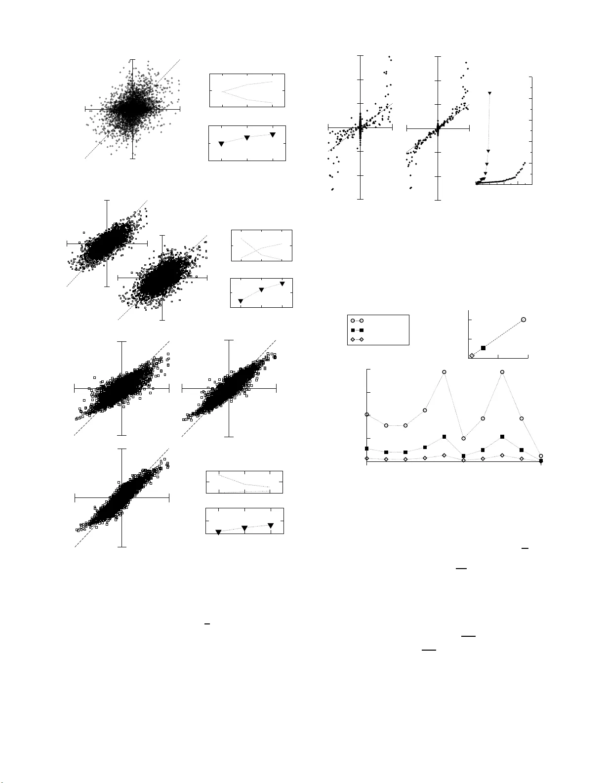
High-Dimensional Inference with the generalized Hopfield Mo del: Principal Comp onen t Analysis and Corr ections S. Co cco 1 , 2 , R. Monasson 1 , 3 , V. Sessak 3 1 Simons Center for Systems Biolo gy, Institute for A dvanc e d Study, Princ eton, NJ 08540, USA 2 L ab or atoir e de Physique St atistique de l’Ec ole Normale Sup ´ erieur e, CNRS & Univ. Paris 6, Paris, F r anc e 3 L ab or atoir e de Physique Th´ eor ique de l’ Ec ole Normale Sup´ er ieur e, CNRS & Univ. Paris 6, Paris, F r anc e W e consider the problem of inferring the interactions betw een a set of N binary v ariables from the knowl edge of their frequencies and pairwise correlatio ns. The inference framew ork is based on the Hopfield model, a special case of the Ising mo del where the interaction matrix is defi ned th rough a set of patterns in the v ariable space, and is of rank muc h smaller than N . W e show that Maximum Likel iho od inference is deeply related to Principal Comp onen t A nal ysis when the amplitude of the pattern components, ξ , is negligible compared to √ N . Using techniques from statistical mechanics, w e calculate the corrections to the patterns to t he first order in ξ / √ N . W e stress th at it is important to generalize the Hopfi el d mo del and include b oth attractive and repulsive patterns, t o correctly infer net works with sparse and strong interactions. W e present a simple geometrical criterion to decide ho w many attractiv e and repulsive patterns s hould b e considered as a function of t he sampling noise. W e moreo ver discuss how many sampled configurations are required for a go od inference, as a function of the system size N and of the amplitude ξ . The inference approach is illustrated on synthetic and biological data. I. INTRO DUCT I ON Understanding the pa tter ns of corr elations b et ween the comp onen ts of complex sys tems is a fundamental issue in v ar ious scientifi c fields, ranging from neurobiolog y to ge- nomic, from finance to so ciology , ... A r ecurren t problem is to disting u ish betw een direct correlatio ns, pro duced by ph ysio logical or functiona l interactions b et ween the com- po nen ts, a nd netw ork correlatio n s, which are mediated by other, third-party compo nen ts. V arious approa c hes hav e b een pr oposed to infer int era ctions fr om corre la - tions, exploiting concepts related to statistical dimen- sional reduction [1], causality [2], the max im um entropy principle [3], Ma r k ov rando m fields [4] ... A ma jor prac- tical and theoretical difficulty in doing so is the pa ucit y and the quality of data : reliable analysis should b e able to unv eil r eal patter ns of interactions, even if measures are affected b y under- o r noisy sa mpling. The size of the interaction netw ork can be comparable to o r la rger than the n umber of data, a situation refer red to a s high- dimensional infere nc e . The purp ose of the present work is to esta blish a quan- titative corr espondence b et ween tw o of those appr o ac hes, namely the inference of Boltzmann Machines (als o called Ising model in statistical ph ysics and undir e cted graph- ical mo dels for discr ete v ariables in statistical inference [4]) and Principal Comp onen t Analysis (PCA) [1]. In- verse Boltzmann Mac hines (BM) are a mathematica lly well-founded but computationally c halleng ing approach to infer interactions fro m cor relations. O ur scop e is to find the in terac tio ns among a set of N v ar iables σ = { σ 1 , σ 2 , . . . , σ N } . F or simplicity , we c onsider v ariables σ i taking bina r y v alues ± 1 o nly ; the discussion b elo w ca n be easily extended to the ca se of a larg er num ber of v al- ues, e.g. to genomics where nucleotides are enco ded b y four-letter symbo ls , o r to proteomics where a m ino- a cids can take tw ent y v alues. Assume that the a verage v alues of the v ar iables, m i = h σ i i , a nd the pa ir wise corr ela- tions, c ij = h σ i σ j i are measur e d, fo r instance, throug h the sampling of, sa y , B configuratio ns σ b , b = 1 , . . . , B . Solving the in verse BM problem cons ists in finding the set of interactions, J ij , a nd of lo cal fie lds , h i , defining an Ising mo del, such that the equilibrium magnetizations and pairwise corr elations coincide with, resp ectiv ely , m i and c ij . Many pro cedures have b een designed to tackle this inv erse pr oblem, including learning algor it hms [5], adv a nce d mean-field techniques [6, 7], messa g e-passing pro cedures [8 , 9], cluster expans io ns [10, 11], gr aphical lasso [4] and its v ariants [12]. The perfor mance (ac c u- racy , running time) of those pro cedures dep end on the structure of the underlying in teraction net work a nd on the qua lit y of the sampling, i.e. how large B is. Principal Comp onen t Analysis (PCA) is a widely po p- ular to o l in statistics to analy ze the cor relation structure of a set of v a riables σ = { σ 1 , σ 2 , . . . , σ N } . The principle of PCA is simple. One star ts with the correla t ion matrix, Γ ij = c ij − m i m j q (1 − m 2 i ) (1 − m 2 j ) , (1) which expres ses the cov a riance b et ween v ariables σ i and σ j , resca led by the pro duct o f the exp ected fluctuations of the v ariables taken separately . Γ is then diagonal- ized. T he pro jections of σ along the top eigenmo des (asso ciated to the largest eigenv alues of Γ) iden tify the uncorrela t ed v ariables which c o n tribute most to the to- tal v a riance. If a few, sa y , p ( ≪ N ), eigenv alues are notably larg er than the re ma ining ones PCA achieves an impo rtan t dimensional r eduction. The determination of the n umber p of comp o nen ts to b e reta ined is a delicate issue. It may b e done b y comparing the spectr u m of Γ to the Marcenko-Pastur (MP) s pectrum for the null hypothesis, that is, for the c orrelation matrix calculated from the s ampling of B configurations o f N independent 2 v ar iables [13]. Generally those tw o sp ectra coincide when N is large , except for s ome large or small eigenv alues of Γ, r etained as the r elev a n t comp onen ts. The a dv a n ta ges o f PCA are m ultiple, which explains its success . The metho d is very versatile and fast as it only requir e s to diag onalize the corr elation matrix, which can be achieved in a time po lynomial in the size N of the problem. In addition, P CA may be extended to incor- po rate prior information about the comp onen ts, whic h is particularly helpful for pr ocessing noisy data. An illus- tration is spar se PCA, which lo oks for principal comp o- nent s with ma n y v anishing entries [1 4 ]. In this pa per we pr esen t a conceptual and practical framework which encompasses BM and PCA in a con- trolled w ay . W e show tha t P CA , with a pp ro priate mo d- ifications, can b e used to infer B M and discuss in detail the amount o f data necessar y to do so. Our framew or k is based on an extension of a c elebrated mo del of statistical mechanics, the Hopfield mo del [15]. The Hopfield model was orig inally intro duced to mo del auto- a ssociative mem- ories, and r elies on the notion of pa tter ns [16]. Informally sp eaking, a pa tt ern ξ = ( ξ 1 , . . . , ξ N ) defines an a ttr activ e direction in the N -dimensional space of the v a riable con- figurations, i.e. a direc tio n alo ng which σ has a tendency to alig n . The norm of ξ c har acterizes the strength of the attraction. While having o nly attractive patterns ma kes sense for auto-a ssociative memories, it is an unneces s ary assumption in the context of BM. W e therefore general- ize the Hopfield mo del by including repulsive patterns ˆ ξ , that is, directions in the N -dimensio n al space which σ tends to b e o rthogonal to [17]. F rom a technical p oint of view, the generalized Hopfield mo del with p a tt ra ctiv e patterns and ˆ p repulsive patterns is simply a par ticular case of BM with an interaction matrix, J , o f rank equal to p + ˆ p . If one knows a prio ri tha t the rank of the true J is indeed small, i.e. p + ˆ p ≪ N , using the generalized Hopfield mo del ra ther than a generic BM a llo ws one to infer muc h less parameter s and to avoid ov erfitting in the presence o f noisy data. W e firs t co nsider the case where the comp onen ts ξ i and ˆ ξ i are very s m all co m par ed to √ N . In this limit ca se we show that Max im um Likeliho od (ML) inference with the generalized Hopfield mo del is closely related to PCA. The attractive patterns ar e in o ne- to-one cor respondence with the larg est comp onen ts of the correla tion matrix, while the repulsive patterns cor respond to the sma llest com- po nen ts, which are no rmally discar ded by PCA. When all patter ns are selected ( p + ˆ p = N ) inference with the generalized Hopfield model is equiv alent to the mean- field a ppro ximation [6]. Retaining only few significative comp onen ts helps, in pr inciple, to remov e noise fro m the data. W e present a simple g eometrical criterion to de c ide in pr actice how many attractive and repulsive pa tt erns should be considere d . W e also addre s s the question of how many samples ( B ) are r equired for the inference to be mea nin gful. W e calc ula te the er ror ba rs ov er the pat- terns due to the the finite s ampling. W e then analyz e the case where the data are s a mpled from a genera lized Hopfield mo del, and infere nce amounts to lea rn the pat- terns o f that mo del. When the system size, N , and the nu mber of s a mples, B , ar e both sent to infinity with a fixed ra t io, α = B N , there is a critical v alue of the ratio, α c , b elo w which lear ning is not poss ible . The v alue of α c depe nds on the amplitude of the pattern comp onent s. This tra n sition corresp onds to the re t ar ded lea r ning phe- nomenon discovered in the con text o f super vised learn- ing with contin uous v ariables and rigo rously studied in random matrix a nd proba b ility theories, see [13, 18, 19] for reviews. W e v alidate our findings o n synthetic data generated from v arious Ising mo dels with known in ter- actions, a nd present applica tions to neurobio logical and proteomic data. In the ca se o f a small system size, N , or of very str o ng comp onen ts, ξ i , ˆ ξ i , the ML patterns do not coincide with the c o mponents identified by PCA. W e ma k e use of tech- niques from the statistical mechanics of disor dered s ys- tems originally int ended to calc ula te a verages ov er en- sembles o f ma tr ices to c ompute the likelihoo d to the sec - ond order in powers of ξ i √ N for a given corr e lation matrix. W e give explicit ex pressions for the ML pa tt erns in terms of non-linear combinations of the eigenv alues and eigen- vectors of the cor relation matrix. These correctio ns ar e v alida ted on synthetic data. F urther more, we discuss the issue of how ma n y sampled co nfi gur ations are necessa ry to improve ov er the lea ding–order ML patterns as a func- tion of the amplitude of the patter n co mponents and of the sy s t em s ize. The plan of the pa per is a s follo ws. In Sectio n II we define the generalized Hopfield model, the Bay esian in- ference framework and list our main results, that is, the expressions of the patterns without and with cor rections, the criterio n to decide the num be r of pa tter ns, and the expressions for the err or bars on the inferred pa tter ns. T ests on synthetic data ar e presented in Section I II. Sec- tion IV is dev oted to the applications to real biological data, i.e recor dings of the neo cortical activit y of a b e- having rat and cons e n sus multi-sequence alignmen t of the PDZ protein domain family . Readers in teres ted in applying our results rather than in their deriv ation need not read the s ub sequent sections. Der iv a tio n o f the log - likelihoo d with the gener alized Hopfield model and of the main inference form ulae can be found in Section V. In Section VI w e study the minimal num b er B of samples necessary to a c hieve an accur ate inference, a nd how this nu mber dep ends on the n umber of patterns and on their amplitude. Persp ectiv es and conclusions ar e given in Sec- tion VI I. II. DEFINITIONS AND MAIN RESUL TS A. Generalized Hopfield Mo del W e cons ider configuratio ns σ = { σ 1 , , σ 2 , . . . , σ N } o f N binary v a riables taking v alues σ i = ± 1, drawn according 3 to the probability P H [ σ | h , { ξ µ } , { ˆ ξ µ } ] = exp − E [ σ , h , { ξ µ } , { ˆ ξ µ } ] Z [ h , { ξ µ } , { ˆ ξ µ } ] , (2) where the energy E is given by E [ σ , h , { ξ µ } , { ˆ ξ µ } ] = − N X i =1 h i σ i − 1 2 N p X µ =1 N X i =1 ξ µ i σ i ! 2 + 1 2 N ˆ p X µ =1 N X i =1 ˆ ξ µ i σ i ! 2 . (3) The partition function Z in (2) ensur es the normaliza - tion o f P H . The co mponents of h = ( h 1 , h 2 , .., h N ) a r e the lo cal fields acting on the v ariables. The patterns ξ µ = { ξ µ 1 , ξ µ 2 , . . . , ξ µ N } , with µ = 1 , 2 , . . . , p , ar e attra c - tive patterns: they define preferred directions in the co n- figuration space σ , along which the ene r gy E decr eases (if the fields a r e weak enough). The patterns ˆ ξ µ , with µ = 1 , 2 , . . . , ˆ p , a re repulsive patterns: configura tions σ aligned along tho se directions hav e a larg er ener gy . The pattern comp onen ts, ξ µ i , ˆ ξ µ i , and the fields, h i , are r eal- v alued. Our model is a genera lized version of the o r iginal Hopfield mo del [15], whic h has o nly attractive patter ns and corres ponds to ˆ p = 0. In the follo wing, we will a s- sume tha t p + ˆ p is muc h smaller than N . Energy function (3) implicitly defines the coupling J ij betw een the v aria bles σ i and σ j , J ij = 1 N p X µ =1 ξ µ i ξ µ j − 1 N ˆ p X µ =1 ˆ ξ µ i ˆ ξ µ j . (4) Note that any interaction matrix J ij can b e written un- der the form (4), with p and ˆ p being, resp ectiv ely , the nu mber o f p ositive and negative eigenv alues of J . Here, we assume that the total num be r of patterns, p + ˆ p , i.e. the rank of the ma t rix J is (muc h) smaller than the s y s- tem size, N . The data to be a nalyzed consists of a set of B config- urations of the N spins, σ b , b = 1 , . . . , B . W e ass um e that tho s e configura tio ns ar e drawn, independently fr om each other, from the distribution P H (2). The para me- ters defining P H , that is, the fields h and the patterns { ξ µ } , { ˆ ξ µ } ar e unknown. Our scop e is to determine the most likely v alues for those fields and pa t terns fr o m the data. In Bay es inference framework the p osterior distri- bution for the fields and the patter ns given the data { σ b } is P [ h , { ξ µ } , { ˆ ξ µ }|{ σ b } ] = P 0 [ h , { ξ µ } , { ˆ ξ µ } ] P 1 [ { σ b } ] (5) × B Y b =1 P H [ σ b | h , { ξ µ } , { ˆ ξ µ } ] , where P 0 enco des some a priori informatio n over the pa- rameters to b e inferred a nd P 1 is a normalization. It is imp ortant to realize that ma n y transfor ma tions af- fecting the patterns ca n actually leave the coupling ma - trix J (4) and the distribution P H unch ang ed. A sim- ple ex a mple is given b y an orthogona l transformation O ov er the attractive patterns : ξ µ i → ¯ ξ µ i = P ν O µν ξ ν i . This inv ar ia nce entails that the the problem of inferring the patterns is not sta t istically consistent : even with an infinite n umber of sampled data no inference pro cedure can distinguish b et ween a Hopfield mo del with patterns { ξ µ } and another one with patterns { ¯ ξ µ } . How ever, the inference of the coupling s is statistica lly consis t ent: tw o distinct matr ices J define tw o distinct distributions ov er the data . In the presence of r epulsiv e patterns the complete in- v ar iance gr o up is the indefinite or thogonal group O ( p, ˆ p ), which has 1 2 ( p + ˆ p )( p + ˆ p − 1) genera t or s. T o select o ne particular set o f mo st lik ely patterns, we e x plicitly break the inv aria nce throug h P 0 . A con venien t choice w e use throughout this paper is to impose that the w eighted dot pro ducts of the pair s of attra ctiv e a nd/ or repulsive pa t - terns v anish: X i ξ µ i ξ ν i (1 − m 2 i ) = 0 1 2 p ( p − 1) co n stra in ts , X i ξ µ i ˆ ξ ν i (1 − m 2 i ) = 0 p ˆ p constra in ts , (6) X i ˆ ξ µ i ˆ ξ ν i (1 − m 2 i ) = 0 1 2 ˆ p ( ˆ p − 1) constraints . In the following we will use the vocable Maximum Like- liho od inference to refer to the c a se wher e the prior P 0 is used to break the in v a riance o nly . P 0 may also b e chosen to imp ose sp ecific co ns t ra in ts on the pattern amplitude, see Section I I E devoted to regulariza tion. B. Maximum Likeliho od Inference: lo west order Due to the absence of three- or higher order- b o dy in- teractions in E (3), P dep ends on the data { σ b } only through the N ma gnetizations, m i , a nd the 1 2 N ( N − 1 ) t wo-spin cov ariances, c ij , o f the sampled da ta : m i = 1 B X b σ b i , c ij = 1 B X b σ b i σ b j . (7) W e consider the cor relation matrix Γ (1), and call λ 1 ≥ . . . ≥ λ k ≥ λ k +1 ≥ . . . ≥ λ N its eigenv alues. v k de- notes the eigen vector atta ched to λ k and normalized to unit y . W e also in tro duce another notation to lab el the same eigen v alues and eigenv ector s in the reverse order: ˆ λ k ≡ λ N +1 − k and ˆ v k = v N +1 − k , e.g. ˆ λ 1 is the small- est eigenv alue of Γ; the motiv ation for doing so will b e transpare nt below. Note that Γ is, b y construction, a semi-definite p ositiv e ma trix: all its eig en v alues ar e p os- itive. In addition, the sum of the eig en v alues is equal to N since Γ ii = 1 , ∀ i . Hence the largest a nd smallest 4 eigenv alues a re guaranteed to be , resp ectiv ely , larger and smaller tha n unity . In the following Greek indices, i.e. µ, ν, ρ , corr espond to integers comprised b et ween 1 and p or ˆ p , while ro man letters, i.e. i, j, k deno te in teger s ranging fr om 1 to N . Finding the patterns and fields maximizing P (5) is a very hard co mputatio nal task . W e in tro duce an approx- imation scheme for those par ameters ξ µ i = ( ξ 0 ) µ i + ( ξ 1 ) µ i + . . . , ˆ ξ µ i = ( ˆ ξ 0 ) µ i + ( ˆ ξ 1 ) µ i + . . . , h i = ( h 0 ) i + ( h 1 ) i + . . . . (8) The deriv a tion of this s y stematic approximation scheme and the discussion of how smalle r the contributions get with the order of the approximation can b e found in Sec- tion V A. T o the lowest or der the patterns ar e given by ( ξ 0 ) µ i = s N 1 − 1 λ µ v µ i p 1 − m 2 i (1 ≤ µ ≤ p ) (9) ( ˆ ξ 0 ) µ i = s N 1 ˆ λ µ − 1 ˆ v µ i p 1 − m 2 i (1 ≤ µ ≤ ˆ p ) . The a bov e express io ns r e quire tha t λ µ > 1 for an attrac- tive pattern and ˆ λ µ < 1 for a repulsive pattern. Once the pa tter ns are computed the int era ctions, ( J 0 ) ij , can be calcula t ed fr om (4), ( J 0 ) ij = 1 q (1 − m 2 i )(1 − m 2 j ) p X µ =1 1 − 1 λ µ v µ i v µ j − ˆ p X µ =1 1 ˆ λ µ − 1 ˆ v µ i ˆ v µ j ! . (10) The v alues of the lo cal fields are then obtained from ( h 0 ) i = tanh − 1 m i − X j ( J 0 ) ij m j , (11) which ha s a straightforw ar d mean-field interpretation. The ab o ve results ar e r eminiscen t of P CA, but differ in s e v eral significative asp ects. Firs t, the patter ns do not coincide with the eigenv ectors due to the pr e s ence of m i -dep enden t terms. Secondly , the presence o f the λ µ -dep enden t factor in (9) discounts the patter ns corre- sp onding to eigenv alues close to unity . This effect is easy to understand in the limit ca se of indep enden t spins and per fect sampling ( B → ∞ ): Γ is the iden tit y matrix, which gives λ µ = 1 , ∀ µ , and the patterns rightly v anish. Thirdly , and mo st imp ortan tly , not o nly the la rgest but also the smallest eig e n mo des must be taken in to account to calcula te the interactions. The coupling s J 0 (10) calculated from the low est-o rder approximation for the pa tt erns a re closely related to the mean-field (MF) interactions [6], J M F ij = − (Γ − 1 ) ij q (1 − m 2 i )(1 − m 2 j ) , (1 2) where Γ − 1 denotes the inv erse matrix o f Γ (1 ) . How ever, while all the eigenmo des o f Γ are ta k en into a ccoun t in the MF interactions (12), our lo west-order interactions (1 0) include c o n tributions from the p largest a nd the ˆ p small- est eig enmodes o nly . As the v a lues of p, ˆ p ca n b e chosen depe nding on the num b er of av ailable data, the g eneral- ized Hopfield int era ctions (10) is a priori less sensitive to ov erfitting. In particular, it is p o ssible to av oid consider- ing the bulk par t of the sp ectrum of Γ, which is essentially due to undersampling ([1 3 ] and Section VI B 2). C. Sampling error bars on the patterns The p osterior distribution P ca n lo cally be approxi- mated with a Gaussian distribution centered in the most likely v alues fo r the patterns , { ( ξ 0 ) µ } , { ( ˆ ξ 0 ) µ } , and the fields, h 0 . W e obtain the cov ariance matr ix of the fluc- tuations of the pa tt erns around their most likely v alues, h ∆ ξ µ i ∆ ξ ν j i = N M ξξ µν ij B q (1 − m 2 i )(1 − m 2 j ) . (13) and identical expressions for h ∆ ξ µ i ∆ ˆ ξ ν j i a nd h ∆ ˆ ξ µ i ∆ ˆ ξ ν j i upo n substitution of M ξξ µν ij with, resp ectiv ely , M ξ ˆ ξ µν ij and M ˆ ξ ˆ ξ µν ij . The en tries of the M matrices are M ξξ µν ij = δ µν N − ˆ p X k = p +1 v k i v k j | λ k − ˆ λ µ | + p X ρ =1 | λ µ − 1 | λ ρ v ρ i v ρ j G 1 ( λ ρ , λ µ ) + ˆ p X ρ =1 | λ µ − 1 | ˆ λ ρ ˆ v ρ i ˆ v ρ j G 1 ( ˆ λ ρ , λ µ ) # + G 2 ( λ µ , λ ν ) G 1 ( λ µ , λ ν ) v µ j v ν i , M ξ ˆ ξ µν ij = G 2 ( λ µ , ˆ λ ν ) G 1 ( λ µ , ˆ λ ν ) v µ j ˆ v ν i , (14) and M ˆ ξ ˆ ξ µν ij is obtained from M ξξ µν ij upo n s ubstit ution of λ µ , λ ν , v µ i , v ν i with, resp ectiv ely , ˆ λ µ , ˆ λ ν , ˆ v µ i , ˆ v ν i . F unc- tions G 1 and G 2 are defined through G 1 ( x, y ) = ( x | y − 1 | + y | x − 1 | ) 2 , G 2 ( x, y ) = p x y | x − 1 | | y − 1 | . (15) The cov a r iance matrix of the fluctuations of the fields is given in Section V D. Error bar s o n the couplings (4) ca n be calcula t ed fr om the ones o n the patter ns . F or m ula (13) tells us how sig nificativ e ar e the infer r ed v alues of the patter ns in the presence o f finite sa m pling. F or insta nce, if the error bar h (∆ ξ µ i ) 2 i 1 / 2 is larg er than, or comparable w ith the patter n comp onen t ( ξ 0 ) µ i calculated from (9) then this comp onen t is statistica lly compatible with zero. Accor ding to formula (13) we ex pect err o r bars of the o rder of 1 √ α ov er the pa tter n comp onen ts, where α = B N . 5 λ θ β ξ ’ v (ξ ) = 0 ’ a v 1− 1 FIG. 1: Geometrical representation of identity (16), exp res s- ing the rescaled pattern ξ ′ as a linear combination of the eigen vector v and of the orth o gonal fluctuations β . The most lik ely rescaled pattern, ( ξ ′ ) 0 , corresp on ds to a = 1 − 1 λ , β = 0.The dashed arc has radius q 1 − 1 λ . The subscript µ has b een dropp ed to lighten notations. D. Optimal num b ers of attractive and repulsive patterns W e now determine the num ber s of patterns, p and ˆ p , based o n a simple geometric criterion; the reader is re- ferred to Section V E for detailed calcula t ions. T o each attractive pattern ξ µ we ass o ciate the rescaled pattern ( ξ µ ) ′ , whose comp onen ts are ( ξ µ i ) ′ = ξ µ i p 1 − m 2 i / √ N . W e write ( ξ µ ) ′ = √ a µ v µ + β µ , (16) where a µ is a p ositiv e co efficien t, and β µ is a vector or- thogonal to a ll rescaled patterns b y virtue of (6) (Fig . 1). Our low est or der form ula (9) for the Maximum Lik eli- ho od estimators giv es a µ = 1 − 1 λ µ and β µ = 0, s ee Fig. 1. This result is, to some extent, misle a ding. While the mo st lik ely v alue for the vector β µ is indeed zero, its norm is a lm os t surely not v anishing! The statement may app ear para do xical but is well-known to hold for sto c hastic v aria bles: while the average or typical v alue of the lo cation of an isotro pic ra ndom walk v a nishes, its av erage sq uared displacement do es not. Here, β µ repre- sents the sto c hastic difference betw een the patter n to b e inferred and the dir e c t ion of one o f the la r gest e ig en vec- tors of Γ. W e ex pect the squared norm ( β µ ) 2 to hav e a non-zero v alue in the N , B → ∞ limit at fixed ratio α = B N > 0. Its av era ge v alue can be straightforw ardly computed fr o m formula (14), h ( β µ ) 2 i = 1 B X i M ξξ µµ ii = 1 B N − ˆ p X k = p +1 1 λ µ − λ k , (17) where µ is the index o f the pattern. W e define the a ngle θ µ betw een the eigen vector v µ and the rescaled pattern ( ξ µ ) ′ through θ µ = sin − 1 s h ( β µ ) 2 i 1 − 1 λ µ , ( 18 ) see Fig. 1. Small v alues of θ µ corres p ond to relia b le pat- terns, while la rge θ µ indicate that the Maximum Like- liho od estimator o f the µ th pattern is plagued b y noise. The v alue of p such that θ p is, say , ab out π 4 is our esti- mate for the num b er of attra ctiv e patterns. The ab o ve a pp ro ac h can be easily re p eated in the case of repulsive patterns. W e obtain, with obvious notations, h ( ˆ β µ ) 2 i = 1 B X i M ˆ ξ ˆ ξ µµ ii = 1 B N − ˆ p X k = p +1 1 λ k − ˆ λ µ , (19) and ˆ θ µ = sin − 1 v u u t h ( ˆ β µ ) 2 i 1 ˆ λ µ − 1 . (20) The v a lue of ˆ p such that ˆ θ ˆ p is, say , ab out π 4 is our estimate for the num b er of repulsive patterns. E. Regularization So far we hav e consider ed that the prior proba bility P 0 ov er the patterns was uniform, and was used to break the inv a r iance through the conditions (6). The prio r pro ba- bilit y can be used to co nstrain the amplitude of the pat- terns. F or instance, w e can in tro duce a Ga ussian prior on the patterns, P 0 ∝ exp " − γ 2 N X i =1 (1 − m 2 i ) p X µ =1 ( ξ µ i ) 2 + ˆ p X µ =1 ( ˆ ξ µ i ) 2 !# , (21) which p enalizes la rge pattern comp onent s [11]. The pres- ence of the (1 − m 2 i ) factor ent ails that the effective strength of the regula rization term, γ (1 − m 2 i ), dep ends on the site magnetiza tio n. Reg ularization is particularly useful in the ca se of severe undersampling. With regula r- ization (21) the lo west or der expression for the pattern is still given by (9), after car rying out the following tr a ns- formation o n the eigenv alues, λ µ → λ µ − γ , ( µ = 1 , . . . , p ) , λ k → λ k , ( k = p + 1 , . . . , N − ˆ p ) , ˆ λ µ → ˆ λ µ + γ , ( µ = 1 , . . . , ˆ p ) . (22) The v alues o f p and ˆ p must be such that the transformed λ p and ˆ λ ˆ p are, res pectively , larger a nd smaller tha n unity . Regulariza tio n (21) ensures that the couplings do not blow up, even in the presence of zero eig en v alues in Γ. Applications will b e presented in Sections I II and IV. The v alue of the re g ularization strength γ can b e chosen based on a Bayesian criterio n [20]. 6 F. Maximum li k eliho od inference: first corrections W e now give the expression for the first-order corr ec- tion to the a ttr activ e patterns, ( ξ 1 ) µ i = s N 1 − m 2 i N X k =1 A kµ B kµ v k i , (23) where A kµ = C k C µ + p X ρ =1 + N X ρ = N +1 − ˆ p ( λ ρ − 1) × X i v k i v µ i ( v ρ i ) 2 + 2 m i C ρ v ρ i p 1 − m 2 i (24) and B kµ = 1 2 q λ µ λ µ − 1 if k ≤ p , √ λ µ ( λ µ − 1) λ µ − λ k if k ≥ p + 1 . (25) and C k = X i m i v k i p 1 − m 2 i p X ρ =1 + N X ρ = N +1 − ˆ p ( λ ρ − 1) ( v ρ i ) 2 . (26) Similarly , the fir st c orrections to the repulsive patterns are ( ˆ ξ 1 ) µ i = s N 1 − m 2 i N X k =1 ˆ A kµ ˆ B kµ v k i . (27) The definition of ˆ A kµ is iden tical to (24), with C µ and v µ i replaced with, resp ectiv ely , C N +1 − µ and ˆ v µ i . Finally , ˆ B kµ = 1 2 q ˆ λ µ 1 − ˆ λ µ if k ≥ N − ˆ p + 1 , √ ˆ λ µ (1 − ˆ λ µ ) ˆ λ µ − λ k if k ≤ N − ˆ p . (28) The fir st order co rrections to the fields h i can b e found in Sectio n V F. It is in teresting to no te that the corrections to the pat- tern ξ µ inv olve non- line a r interactions b e tw een the eig en- mo des of Γ . F or m ula (2 4) for A kµ shows that the mo des µ and k interact thro u gh a m ulti-b ody overlap with mo de ρ (pro vided λ ρ 6 = 1). In addition, A kµ do es not a pri- ori v anish for k ≥ p + 1 : corr ections to the pa tt erns hav e non–zero pro jections ov er the ’noisy’ modes of Γ. In other w or ds, v alua ble information ov er the true v alues of the patterns can be extracted fro m the eigenmo des of Γ a ssociated to bulk eige nv alues. G. Quality of the i nference vs . size of the data set The a ccuracy ǫ on the inferr ed pattern is limited b oth by the sampling error resulting from the finite num b er of data and the in trinsic er ror due to the expansion (8). According to Section II C, the sa mplin g erro r on the pat- tern comp onent is expec t ed to decrease as ∼ q N B . T he int rinsic er ror depends o n the order o f the expansion, on the size N and on the amplitude of the pa tt erns . No inference is p ossible unless the ratio α = B N exceeds a critica l v alue, referred to as α c in the following (Sec- tion VI A 2). This phenomenon is s imilar to the retarded learning phase transition discovered in the context of un- sup e rvised le arning [18]. Assume tha t the patter n co mponents ξ i are o f the or- der of one (compared to N ), that is, that the couplings are almos t all non zero and of the order of 1 N . Then, the int rinsic error is of the o rder of 1 N with the low est or- der for m ula (9), a nd of the order of 1 N 2 when cor r ections (23) are taken into account; for a more precise statement see Section V A and for m ula (49). The co rresponding v alues of B at which saturation takes place ar e, resp ec- tively , of the order of N 3 and N 5 . The behaviour of the relative error b et ween the true and inferred patterns, ǫ (32), is summar ized in Fig. 2. In g eneral w e exp ect that B ∼ N 1+2 a samples at least are required to ha ve a mor e a ccurate inference with a th -order patterns than with ( a − 1) th -order patterns. F urthermor e there is no need to sample more tha n N 3+2 a configuratio ns when using the a th -order expr ession for the patter ns. If the system has O ( N ) no n v a nishing couplings J ij of the order of J , then patterns hav e few large comp onen ts, of the o rder of √ J . In this case the intrisic err or over the patterns will b e of the or der of J with the low est o rder inference for m ula e, and of the order of J 2 with the firs t correctio ns. The n umbers of sampled configurations, B , B 5 −2 −1 1 ~ (N/B) 1/2 with corrections lowest order N N N N N 3 ε FIG. 2: Schematic b eha viour of th e error ǫ on the inferred patterns as a function of th e number B of sampled configu- rations and for a problem size equal to N , when th e pattern compon ents are of the order of unity compared to N . See main tex t for the case of few large pattern comp onen ts, of the order of √ N , i .e. couplings J of th e ord er of 1. 7 required to r eac h those minimal error s will b e, resp ec- tively , of the or der of N J 2 and N J 4 . II I. TEST S ON SYNT HET IC DA T A In this Section we test the formulae of Section II for the patterns and fields aga inst synthetic da t a generated from v ario us Ising mo dels with known interactions. W e consider four mo dels: • Mo del A is a Hopfield mo del with N = 10 0 spins, p (= 1 or 3) attractive patterns and no repuls iv e pattern ( ˆ p = 0). The comp onen ts of the patter ns are Gaussian ra ndom v a riables with zero mean and standard deviation ξ , sp ecified later. The lo cal fields h i are s e t eq ua l to zero. • Mo del B: Mo del B consists of N spins, group ed int o four blo cks o f N 4 spins each. The p = 3 pat- terns have uniform components over the blo c ks: ξ 1 = 2 √ 3 5 (0 , 1 , 1 , 1), ξ 2 = 2 5 ( √ 3 , 1 , − 2 , 1), ξ 3 = 2 5 ( √ 3 , − 2 , 1 , 1 ). The fields ar e set to zero. Those choices ensure that the pa tter n are orthogonal to each other, and hav e a weak intensit y: on average, | ξ | 2 = 9 25 < 1. • Mo del C is a very simple Ising mo del where all fie lds and couplings v anis h, except coupling J 12 ≡ J b e- t ween the fir st tw o spins. • Mo del D is an Ising model with N = 5 0 spins, on an Erdos - Ren yi rando m graph with av era ge con- nectivity (num b er of neighbor s for each s pin ) equal to d = 5 and coupling v alues J distributed uni- formly b et ween -1 and 1. Model D is an insta n ce of the Viana-Br a y mo del [21]. In the thermo dynamic limit N → ∞ this mo del is in the s pin glass phase since d h tanh 2 ( J ) i J > 1 [21]. F or each o ne of the mo dels ab o ve, the magnetiza tions and pair w is e correla tions can b e estimated throug h the sampling of B configuratio ns at equilibr ium using Monte Carlo sim ulations. This allows us to estimate the conse- quence of sampling nois e on the infer e nce quality by v ary - ing the v a lue of B . F urther mo re, for mo dels B and C , it is p o ssible to obtained the exact Gibbs v alues for m i and c ij (corresp onding to a p erfect sampling, B = ∞ )[40]. This allo ws us to study the systematic erro r resulting from formulae (9,23,27), irresp ectiv ely of the sampling noise. Mo del A is used to tes t the lower o rder formu la for the patterns, and how the quality of inference dep ends on the amplitude of the patter ns . Mo dels C and D are highly diluted netw ork s with strong J = O (1 ) in terac- tions, while mo dels A a nd B corre spond to dense net- works with weak J = O ( 1 N ) couplings. Mo dels C and D ar e, therefore, harder benchmarks for the g eneralized Hopfield mo del. In addition, the couplings implicitly de- fine, thr o ugh (4), b oth attra ctiv e and repuls ive patterns . -0.05 0 0.05 -0.05 0 0.05 -2.5 0 2.5 -2.5 0 2.5 -0.05 0 0.05 -0.05 0 0.05 -2.5 0 2.5 -2.5 0 2.5 inferred ξ i true ξ i true J ij inferred J ij B=40 B=400 FIG. 3: Application of form ula (9) to t wo sets of B = 40 (top) and 400 (b ottom) confi g urations, randomly generated from the d istribu t i on P H (2) for mo del A with p = 1 pattern. The stand a rd dev i ation of the pattern components is ξ = . 7. Left: comparison of the true and inferred couplings for eac h pair ( i, j ). Right: comparison of the true and inferred compon ents ξ i of the pattern, with the error b ars calculated from (13). The dashed lines hav e sl op e unity . In f erence is done with p = 1 attractive pattern and no repu l sive pattern. Those mo dels can th us b e use d to determine how muc h repulsive patterns are requir ed for an accur ate inference of gener a l Ising mo dels. A. Dominant order form ula for the patterns W e start with Mo del A with p = 1 pattern. In this case, no am biguity ov er the inferred pattern is p ossi- ble since the energy E is not inv ariant under contin u- ous tra nsformations, see Section II A. W e may therefore directly compare the true and the inferr ed patterns . Fig- ures 3 and 4 show the accur acy o f the low est order for - m ula for the patter ns, eqn (9). If the pattern comp onen ts are weak, each sampled co nfiguration σ is weakly aligned along the pattern ξ . If the num b er B of sampled c o nfig- urations is small, the larg est eigen vector of Γ is uncor re- lated w ith the patter n dir ection (Fig. 3). When the siz e of the data set is sufficien tly large, i.e. B > α c N (Sec- tion VI A 2), formula (9) captures the rig h t direction of the pattern, and the infer r ed co uplings are re p res en tative of the true interactions. Conv ersely , if the amplitudes o f the comp onen ts of the pattern ξ are s t ro ng enough, each sampled configura t ion σ is likely to b e a ligned along the pattern. A small n umber B (compare d to N ) of those configuratio n s suffice to determine the pattern (Fig. 4). In the latter ca se, we see that the large st comp onen ts ξ i are s ystematically underestimated. A systematic s tudy of how larg e B should b e for the inference to b e reliable can b e found in Section VI. 8 -0.05 0 0.05 -0.025 0 0.025 -4 -2 0 2 4 -2 0 2 -0.05 0 0.05 -0.025 0 0.025 -4 -2 0 2 4 -2 0 2 inferred ξ i true ξ i true J ij inferred J ij B=40 B=400 FIG. 4: Same as Fig. 3, but with a standard deviation ξ = 1 . 3 instead of ξ = . 7. The amplitude is strong enough to magnetize the configurations along the pattern, see Sections VI A 1 and V I B 3. W e no w use model B to genera te the da ta . As mo del B includes more tha n o ne pattern, the infer red patterns cannot b e compa red to the true one easily due to the in- v ar iance o f Section I I A. W e ther efore c ompare in Fig. 5 the true couplings and the interactions found using (9) for three sizes, N = 5 2, 10 0 and 2 00. The size N sets also the a mp litude o f the couplings, which decreases as 1 N from (4). As the pa tter ns are uniform among each one of the four blocks there a re ten p ossibles v alues for the co uplings J ij , dep ending on the lab els a and b of the blo c ks to which i and j b elong, with 1 ≤ a ≤ b ≤ 4. F or N = 100 spins, the relative errors rang e b et ween 3 and 5.5%. When the num b er of spins is do ubled (r espec- tively , halved) the rela tive errors are a b out twice smaller (resp ectiv ely , larger). This r esult confirms that form ula (9) is exact in the infinite N limit only , and that correc- tions of the order of O ( 1 N ) a re expec t ed for finite system sizes (Inset of Fig. 5). This scaling w as expected from Section II G. W e now co nsider mo del C. F or p erfect sampling ( B = ∞ ) the corre la tion matrix (1) is Γ = 1 tanh J 0 . . . 0 tanh J 1 0 . . . 0 0 0 1 . . . 0 0 . . . 0 1 0 0 . . . 0 0 1 . (29) The top eig en v alue, λ 1 = 1 + tanh J > 1, a nd the s m alles t eigenv alue, ˆ λ 1 = λ N = 1 − tanh J < 1, ar e attached to 1 10 block (a,b) 0 0.02 0.04 0.06 0.08 0.1 0.12 ∆ J ab / J ab N = 52 N = 100 N = 200 0 0.01 0.02 1/N 0 0.04 0.08 average ∆ J/J FIG. 5: Relativ e differences b et we en th e tru e and the inferred couplings, ∆ J ab /J ab for three system sizes, N . The inference w as done using the lo wes t order ML formula e ( 9 ) for the pat- terns. Data were generated from Mo del B (perfect sampling); there are a priori ten distinct val ues of the couplings, one for eac h pair of blo c ks a and b . Inset: av erage v alue of ∆ J ab /J ab as a function of 1 N . Circles, squ ar es and diamonds corresp ond to, resp ectiv ely , N = 52, 100 and 200 spins. the eig en vectors v 1 = 1 √ 2 1 1 0 . . . 0 , ˆ v 1 = 1 √ 2 1 − 1 0 . . . 0 . (30) The r emaining N − 2 eige nv alues are eq ual to 1. Using formula (10) for the low est order co upling, J 0 , we find that those eig enmodes do not contribute and that the in- teraction can ta ke three v alues, dep ending on the choices for p and ˆ p : ( J 0 ) p =1 , ˆ p =0 = tanh J 2 (1 + tanh J ) ≃ J 2 − J 2 2 + J 3 3 + . . . , ( J 0 ) p =0 , ˆ p =1 = tanh J 2 (1 − tanh J ) ≃ J 2 + J 2 2 + J 3 3 + . . . , ( J 0 ) p =1 , ˆ p =1 = tanh J 1 − tanh 2 J ≃ J + 2 J 3 3 + . . . . (31) Those expres sions are plotted in Fig. 6. The coupling ( J 0 ) 1 , 0 (dashed line), co rrespo n ding to the standar d Hop- field mo del, saturates at the v alue 1 4 and do es not di- verge with J . E v en the small J behavior, ( J 0 ) 1 , 0 ≃ J 2 , is erroneous. Adding the repulsive pattern lea ds to a visible improv ement, a s fluctuations of the spin config- urations along the eigen vector ˆ v 1 (one spin up a nd the other down) a re p enalized. The inferred c o upling, ( J 0 ) 1 , 1 (bo ld line), is no w cor rect for small J , ( J 0 ) 1 , 1 ≃ J , and diverges for large v alues o f J . 9 -2 -1 0 1 2 J -2 -1 0 1 2 J 0 J 0 = J p=1, p=0 p=1, p=1 p=1, p=0, corr. p=0, p=1 ^ ^ ^ ^ FIG. 6: I nfer red coupling J 0 b et w een the first tw o spins of Model C, within lo west order ML, and as a function of the true coupling J . V alues of p and ˆ p are show n in the Figure. -1 -0.5 0 0.5 1 -1 -0.5 0 0.5 1 p=9 -1 -0.5 0 0.5 1 -2 -1 0 1 2 p=35 p=9 ^ FIG. 7: Inferred vs. true couplings for Mo del D, with B = 4500 sampled configurations. Left : Hopfi eld model with p = 9 (corresp onding to th e opt imal num b er of patterns se- lected by the geometrical criterion); no repulsive p attern is considered ( ˆ p = 0). Righ t: Generalized Hopfield mo del with ( p, ˆ p ) = (9 , 35) (optimal numbers). W e no w turn to Mo del D. Figure 7 compare s the in- ferred and tr ue couplings for B = 4500 s a mpled config- urations. The gener alized Hopfield mo del outp erforms the standard Hopfield mo del ( ˆ p = 0), showing the im- po rtance of repulsive patterns in the inference of spar se net works with str ong in tera c t ions. Large couplings, ei- ther p ositive or negative, are ov erestimated by the lowest order ML estimators for the pa t terns. B. Error bars and criterion for p, ˆ p An illustr a tion of form ula (13) for the error bars is shown in Fig. 3, wher e we compar e the comp onen ts of the true pattern used to gener ate data in Mo del A with the inferred o ne, ( ξ 0 ) i , and the err or bar, p h (∆ ξ i ) 2 i . F or small α = B N the inferred pattern co mponents a re unco r- related with the true pa tter n a nd compatible with zero within the error bars. F or larg e r v alues of α , the discrep- ancy b et ween the inferred and the true comp onen ts a re sto c hastic quant ities of the order of the ca lculated err or bars. W e rep ort in Fig. 8 the tests of the criterion for de- termining p and ˆ p on a rtificially g enerated data fro m an extension of mo del A with p = 3 patterns. F o r very po or sampling (Fig. 8, top) the angle θ 1 is close to π 4 : even the first pattern ca nn ot b e inferre d correctly . This pre- diction is confirmed by the very p oor comparison of the true in teractions and the inferred co upling s calculated from the fir st inferred pattern. F or mo derately accur ate sampling (Fig. 8 , middle) the s tr ongest pattern can be inferred; the accuracy on the inferr ed couplings w orsens when the second pattern is added. Ex cellen t sampling allows for a go o d inference of the structure o f the under- lying mo del: the angle θ µ is s mall for µ = 1 , 2 , 3 (Fig. 8, bo tt om), and larger than π 4 for µ ≥ 4 (not s hown). Not surprisingly large co uplings are systematically affected by error s. Thos e error s can b e corr e c t ed b y taking into account O ( ξ √ N ) co rrections to the pa tter ns if the num b er of data, B , is large eno ugh (Section VI). Figure 9 compares the inferred a nd true couplings for B = 4500 sampled configurations of Mo del D. The opti- mal num ber of patterns given by the geometr ical cr iterion is ( p = 9 , ˆ p = 35), see Fig. 7. Hence most of the comp o- nent s of Γ are retained and the interactions inferred with the g eneralized Hopfield mo del do not differ much from the MF couplings. C. Corrections to the patterns F or m ula (23) for the corrections to the patterns w as tested on mo del B in the case o f p erfect sa mpling. Re- sults a re rep orted in Fig. 1 0 and show that the er rors in the inferr ed couplings ar e m uch smaller than in Fig. 5. Inset of Fig. 10 shows that the relative error s ar e of the order of 1 N 2 only . This scaling w as exp ected from Sec- tion I I G. Pushing our expansion of ξ to the next order in powers of 1 N could in principle give explicit expressio ns for those co rrections. W e hav e also tested our hig he r or- der formula when the fields h i are non-zero. F or instance we hav e consider ed the same Hopfield model with p = 3 patterns as ab o ve, a nd with blo c k pseudo-mag netizations t = 1 15 (2 √ 3 , 2 , 2 , − 4 ). Hence, t was orthogonal to the patterns, and the field comp onen ts were s imply g iv en by h i = tanh − 1 t i , according to (3 8 ) [41]. F or N = 5 2 spins the r elativ e err or over the pseudo- m ag netizations (aver- 10 -0.05 0 0.05 true J -0.05 0 0.05 inferred J B=20 a a a b b b 1 2 3 0 0.5 1 1 2 3 µ 0 0.5 1 θ x 2/ π p=1 -0.05 0 0.05 -0.05 0 0.05 a a a b b b 1 2 3 0 0.5 1 1 2 3 µ 0 0.5 1 θ x 2/ π -0.05 0 0.05 -0.05 0 0.05 p=1 B = 200 p=2 -0.05 0 0.05 -0.05 0 0.05 a a a b b b 1 2 3 0 0.5 1 -0.05 0 0.05 -0.05 0 0.05 -0.05 0 0.05 -0.05 0 0.05 1 2 3 µ 0 0.5 1 θ x 2/ π B = 2000 p=1 p=2 p=3 FIG. 8: Criterion to decide the number p of patterns and p erf ormance of the ML inference p rocedure for th ree different sizes of the data set, B . Left: inferred vs. true interactions with p = 1 , 2 or 3 patterns; the dashed line has slop e u nit y . Right : co efficien ts a µ = ( ρ µ ) 2 and b µ = h ( β µ ) 2 i vs. pattern index µ , and angles θ µ , div i ded by π 2 , see definitions (16) and (18). F or eac h v alue of B one d ata set w as generated from Mo del A with p = 3 patterns, and standard dev i ations ξ 1 = . 95, ξ 2 = . 83, an d ξ 3 = . 77. -1 0 1 -3 -2 -1 0 1 2 3 p=9 p=10 ^ -1 0 1 -3 -2 -1 0 1 2 3 p=11 p=39 ^ 0 10 20 30 40 µ 0 0.1 0.2 0.3 0.4 0.5 θ x2/ π FIG. 9: Inferred vs. true couplings for Mo del D, with B = 4500 sampled configurations. Left: Generalized Hop- field mo del with ( p, ˆ p ) = (9 , 10) and (11 , 39) (corresponding to the num b ers of eigenv alues, resp ective ly , larger and smaller than unity). Right: an gles θ µ and ˆ θ µ for, resp ectiv ely , at- tractive (triangle) and repulsive (diamond) patterns. 1 10 block (a,b) 0 0.002 0.004 0.006 0.008 ∆ J ab / J ab N = 52 N = 100 N = 200 0 0.0002 0.0004 1/N 2 0 0.002 0.004 average ∆ J/J FIG. 10: Relative differences b e tw een the t rue and the in- ferred couplings, ∆ J ab /J ab as a function of the system size, N . The inference wa s done using the fi nite– N ML for mu- lae ( 9) and (23) for th e patterns. Data were generated from a p erfect sampling of the equilibrium d i stribution of a Hop- field mod el with p = 3 patterns and four blo c ks of N 4 spins, see main text; a and b are th e blo c k indices. Inset: av erage v alue of ∆ J ab /J ab as a function of 1 N 2 . Circles, squares and diamonds corresp ond to, resp ectiv ely , N = 52, 100 and 200 spins. aged ov er the four blo c ks a ) w as ∆ t a t a ≃ . 0301 with the large- N for mula (9 ) and ∆ t a t a ≃ 0 . 0 029 with the finite- N formulae (23) and (78). Correctio n s to the PCA were a lso tested when da t a a re corrupted by sampling noise. W e compa re in Fig. 11 the comp onen ts of the pattern of Mo del A found with the low est or der approximation (9) a nd with our first order 11 -4 -2 0 2 4 -4 -2 0 2 4 -4 -2 0 2 4 true ξ i -4 -2 0 2 4 inferred ξ i B = 40 B = 400 FIG. 11: T rue v s. inferre d components of the p a tterns, ξ i , for the mo del with N = 100 spins describ ed in Fig. 4. F ull circles are the result of the low est order inference formula (9), while empty circles sho w the outcome of th e fi rst order form ulae (23). formulae (2 3 ) (case of stro ng patter n) . A clear impr o ve- men t in the quality o f the inference is observed, ev en when the sampling nois e is stro ng. Our seco nd example is Mo del B. W e show in Fig. 1 2 the relative er rors ǫ J = 2 N ( N − 1) X i 0. Hamiltonian (3) with p = 1 pa tt ern is inv a r i- ant under the exchange o f the spin co nfiguration a nd the pattern: E [ σ , 0 , ξ ] = E [ ξ , 0 , σ ]. Our infere n ce problem can thus b e mapp ed onto a dual Hopfield mo del, where the no rmalized inferred pattern, ξ / ˜ ξ , plays the ro le of the dua l spin config uration and the sa mpled spin con- figurations, σ b , b = 1 , . . . , B corresp ond to the B dual 19 0 10 20 30 B 0 0.2 0.4 0.6 0.8 1 S/N 0 100 200 300 10 -20 10 -15 10 -10 10 -5 10 0 0 2 4 6 8 α =B/N 0 0.2 0.4 0.6 0.8 1 S/N 0 2 4 6 8 0 1 r -1/B c (a) (b) N=10 N=20 α c FIG. 17: Entropy of the posterior d i stribution for th e p at- terns, S ( i n bits and p er comp onen t), as a function of the num b er of sampled configurations, B , when the local fields h i are know n to v anish. (a). F erromagnetic regime ( ˜ ξ 2 = 1 . 1): the entrop y decays ex ponentiall y with B . In set: compari- son with the theoretical prediction exp( − B /B c ) (dashed line), with B c ≃ 6 . 85, in semi-log scale. (b). P aramagnetic regime ( ˜ ξ 2 = . 5): S (86) is a decreasing function of α = B / N . The entropies calculated from numerical calculations are shown for N = 10 and N = 20. Inset: the overl ap r (83) b et ween the inferred and true patterns is p ositiv e when α exceeds α c = 1 (87). patterns. In pa rticular, the p osterior entrop y S is equal to the entropy o f the dual Hopfield mo del at inv erse tem- per ature β = ˜ ξ 2 . (80) The duality prop ert y allows us to exploit the well- understo od physics of the Hopfield mo del [27] to simplify the study of our inference problem. 1. Str ong c omp onents In the fer r omagnetic regime ( ˜ ξ > 1), the dual spin configuratio n is strong ly mag ne tize d along the dual pa t - terns. Going back to the inference problem, we find that the ov erla p b et ween the inferred patter n and a sampled configuratio n , q b = X { σ b } , ξ P [0 , ξ |{ σ b } ] Y b P H [ σ b , ˜ ξ ] 1 N X i ξ i σ 1 i , (81) may take v alues + q or − q , where q is the p ositiv e ro ot of q = tanh( q ˜ ξ 2 ). The sign of the ov erlap q b is random, depe nding on whic h one of the tw o states with opp o- site magnetiza tions the configuration σ b in sampled in; it is equal to + or − with equa l probabilities 1 2 . These statements hold if the thermo dynamical limit, N → ∞ , is taken while B is kept fixed. W e find that S is eq ual to the en tro py of a single spin a t inv erse temp erature β , int era cting with B other spins of magnetiza tio n q , S = B X b =0 B b 1 + q 2 b 1 − q 2 B − b S ( B − 2 b ) q ˜ ξ 2 , (82) where S ( u ) = log(2 cosh u ) − u tanh u . Figure 17A shows that the en tro py is almost a pure exp onen tial: lo g S ≃ − B /B c where the decay constant, B c = 1 / log cosh( q ˜ ξ 2 ), is finite (compared to N ). In the ferromagnetic regime few sampled config urations are sufficient to determine ˜ ξ accurately . This result also applies to the ca se of a single ferro- magnetic state. If the field h does not stric t ly v anish and ex plic itely breaks the reversal symmetry b et ween the t wo sta t es, all configuratio ns are s a mpled from the s ame state, with pro babilit y 1 − exp( − O ( N )). Remark a bly , expression (8 2 ) for the entrop y still ho lds. Again we find that B = O (1 ) configurations are sufficient to infer the pattern. W e w ill dis c uss in mo re details the inference in the ferr omagnetic re g ime in Sec tio ns VI B 1 and VI B 3. 2. We ak c omp onents In the pa r amagnetic phase ( ˜ ξ < 1), the overlap (81) betw een the inferred pattern and an exa mple is typically very small, q ∼ N − 1 / 2 . No inference is p ossible unless the nu mber of examples, B , scales linearly with N ; w e denote α = B / N . In this r e gime, w e exp e c t the entropy to b e self-av erag ing: S [ { σ b } ] do es not dep end on the detailed comp osition of the data set and is a function of the v alue of the macrosco pic par ameters, e.g. the ra t io α , o nly . T o calculate this function S we use the r eplica metho d [16, 27]. W e repo rt b elow the results of the replica sy mm etric calculation; tec hnical details can b e found in App endix. The order para meter is the av erage ov erla p r b et w een the inferred and the true patterns, r = X { σ b } , ξ P [0 , ξ |{ σ b } ] Y b P H [ σ b , ˜ ξ ] 1 N X i ξ i ˜ ξ i . (83) which is solution o f the self-consistent equa tion r = Z ∞ −∞ D z tanh( z √ γ + γ ) , (84) 20 where D z = dz √ 2 π e − z 2 / 2 is the Gaussian mea sure, and γ = αβ 2 r (1 − β )(1 − β + β r ) . (85) The p osterior entropy is equal to S = Z ∞ −∞ D z log 2 co sh ( z √ γ + γ ) − α 2 log(1 − β + β r ) − αβ (1 − β − r + 3 β r ) 2(1 − β )(1 − β + β r ) , (86) and is plotted in Fig. 17B. T o check this analytical pre- diction we ha ve run extensive n umerical simulations on small-size systems ( N = 10 , 20). The n umerica l proc e- dure follows three s teps : 1 . ev aluate the partition func- tion Z in (2) thr ough a n exact enumeration; 2. g enerate a data set o f B = αN configurations { σ b i } accor ding to the Hopfield measure P H by rejection sa mp ling; 3. ev alu- ate P 1 in (5) and S in (79) thro ugh exa ct enumerations. The resulting en tropy , av eraged over one hundred data sets, is compatible with the a nalytical predictio n and the existence of 1 N finite-size effects. Inset of Fig. 1 7B shows that the ov erlap r rema in s n ull un til α r eac hes the cr itical v alue α c = 1 ˜ ξ 2 − 1 2 . (87) Hence, in the r ange [0; α c ], the p osterior probability b e- comes more concentrated ( S decrea ses), but not aro und the true pattern ˜ ξ . The existence of a lagg ing phase be - fore any meaningful inferenc e is po ssible is similar to the ’retarded learning’ phenomenon discovered in the field of unsupe r vised lea rning, where the v a r iables to be learned are r eal-v alued [28 – 30]. In the present ca se of binary spins we exp ect the replica symmetric assumption to break do wn at larg e α . The en tro py (86) indeed b e- comes negative when α > α 0 ≃ 42 for the case studied in Fig. 17B. Nevertheless w e may conjecture that the en- tropy decays as S ∼ 1 α when α → ∞ . The dual Hopfield mo del has r andom couplings J ij , with sec o nd momen t equal to h J 2 ij i − h J ij i 2 = α N . Hence T = 1 √ α sets the temper ature scale of the dual mo del. The lo w temp era- ture s c a ling o f the entrop y of the Sher rington-Kirkpatrick (SK) mo del sugg ests that S ∝ T 2 [31]; this s caling is compatible with the small– N results of Fig. 1 7B. Ho w- ever the dual and SK mo dels are not strictly ide ntical when α → ∞ : the coupling matrix J of the dual mo del is guaranteed to be semidefinite po sitiv e, while the en- tries of J are indep enden t in the SK mo del. A c o mplete calculation of the e ntropy v alid for any (large) α would require a replica symmetry broken Ansatz for the order parameters [3 2 ], and is b ey ond the scop e of this article. Note that the calcula t ions above can be extended to real patterns; β in (80) is then replac e d with h ξ 2 i , where the av erage is taken ov er the pa tter n comp onen ts. The ent ro p y is not co ns t ra ined to b e p ositive as in the bi- nary ca se. The distinctio n betw een the s tr ong- and weak- comp onen t regimes rema in s qualitatively unc hang e d , and so do es the v alue of the cr itical r atio α c (87), which does not dep end on the third and higher moments o f ˜ ξ i . B. General case of unkno wn patterns and fie l ds In this Section, w e first interpret the ab o ve results. W e sho w that, while B = O (1) c o nfigurations can be sufficient in a par t icular context, B = O ( N ) data are generally necessary for the inference to be sucessful. The connection betw een the res ults of Section VI A and ran- dom matrix theory a r e emphasiz ed. 1. Infer enc e fr om the m agnetizations Consider first the case where a single state exists, i.e. equations (53) admit a single solution { q µ } ; the case where sta t es co exist will b e discussed in Sectio n VI B 3. F or large N , the av erag e v alue of s pin i with the mea sure P H (2) is m i = tanh h i + X µ q µ ξ µ i . (88) As the err or on the estima te of m i decreases as ∼ q 1 − m 2 i B with B , O (1) configuratio ns are sufficient to sample the magnetizations accurately . F ew sampled configurations therefore give a ccess to the knowledge of a linear combi- nation of the field v ector and pattern v ectors with non zero-overlaps q µ . This linear combination is simply T 0 i , and equatio n (88) coincides with (55). When the fields h i are known and the mo del cons is ts of a single stro ng pattern ( p = 1) the pa tt ern comp onen ts ξ 1 i can b e rea dily calcula ted fr om the magnetizatio ns (88) through ξ 1 i = 1 q tanh − 1 m i where q 2 = 1 N X j m j tanh − 1 m j . (89) This par ticula r case was encountered at the end of Sec- tion VI A 1, when the fields h i are sent to zero after hav- ing broken the reversal symmetry o f the system to avoid state co existence. In the generic situation of unknown fields a n d pa tter ns, knowledge o f the magnetiza tio ns do es not suffice to determine the field and the patterns, and m ust be supplemented with the information coming from the co rrelation matrix Γ ij . 2. Infer enc e fr om the c orr elations: r elationship with r andom matrix the ory What is the order of magnitude o f Γ ij ? W e fir st con- sider the ideal case of p erfect sampling ( B → ∞ while N is large but finite). As a result of the prese nc e of the 21 patterns in the energy (3) the spins are correla t ed. The ent ries of the correla t ion matrix are, for larg e N [42], Γ ij = δ ij + 1 N ξ i ξ j q (1 − m 2 i )(1 − m 2 j ) 1 − 1 N P k ξ 2 k (1 − m k ) 2 (90) where we have considered the c ase of a single pattern ( p = 1 , ˆ p = 0) to lighten notations . Though the patter n affects each correla t ion Γ ij by O ( 1 N ) only , these sma ll contributions a dd up to bo ost the la rgest eigenv alue fro m one (in the abs e nce of pattern) to L = 1 1 − 1 N P k ξ 2 k (1 − m k ) 2 . (91 ) The eigenvector attached to L has comp onen ts v i ∝ ξ i p 1 − m 2 i and ML inference p erfectly re c o vers the pat- tern. In the pres ence of sa mpling noise (finite B ), each cor re- lation (90) is c orrupted b y a sto c hastic term of the or d er of x = 1 √ B . This stochastic term will, in turn, pro duce an ov erall contribution o f the o rder of x √ N = 1 √ α to the larg est eigenv alue. Intuitiv ely , whether α is lar ge or small compared to L − 2 should tell us how hard or easy it is to extra ct the pattern ξ fro m Γ. Several studies in the ph ysics [33, 34] a nd in the mathematics [35] liter atures hav e indeed fo und that an abr upt phase transition takes place at the critical ra t io α c = 1 ( L − 1) 2 . (92) It is a simple chec k that α c coincides with the ratio (8 7 ) for the r etarded lear ning transition ca lc ula ted in Sections VI A 2. In the strong noise regime ( α < α c ) the large s t eigen- vector v 1 of Γ is uncorrela ted with (orthogonal to) the pattern ξ , and the spectrum of Γ is identical to the one of the s ample corr elation matrix o f indepe ndent s pins , whose density of eigen v alues is giv en by the Marcenko- Pastur (MP) law, ρ M P ( λ ′ ) = v (1 − α ) δ ( λ ′ ) + α 2 π λ ′ q v ( λ + − λ ′ )( λ ′ − λ − ) (93) with v ( u ) = ma x ( u, 0) [19]. The edges of the contin uous comp onen t of the MP spec t rum are given by λ ± = 1 − 1 √ α 2 . (94) The lar gest eigenv alue o f Γ, λ + , is no t r elated to the v alue of L . In the w eak noise r egime ( α > α c ) the largest eigen- v alue of Γ is [3 5] λ 1 = L 1 + 1 α ( L − 1) . (95) It exceeds L for any finite α , and conv erg es to L when α → ∞ . The rest of the sp ectrum is describ ed by the MP density (93). Express ion (74) for the s quared no rm b 1 of the orthogona l fluctuations leads to the a nalytical formula b 1 = 1 α Z λ + λ − dλ ′ ρ M P ( λ ′ ) λ 1 − λ ′ = λ 1 − L λ 1 , (96) where we hav e used the analy tica l expressio n of the Stieltjes transform of ρ M P [13]. Using (75) we deduce the v alue of the sq uared pro jection of the inferred rescaled pattern ( ξ 1 ) ′ onto v 1 , a 1 = L − 1 λ 1 . (97) Ident ities (96 ) and (97) are graphica lly interpreted in Fig. 1: b 1 is the square d norm of the orthog onal fluctua- tions β , while a 1 is the squared pro jection of the rescaled pattern ξ onto v 1 . The ab o ve discuss ion is illustrated on the simple ca s e of a Hopfield mo del with p = 1 , ˆ p = 0 patterns in Fig. 18, see caption for the description of the model. Using for- m ula (91) we compute the largest eigenv alue of the cor- relation matrix for p erfect sa mpling, L = 2. Figure 18 shows that a lar ge eigenv a lue c learly pulls out fro m the bulk s pectrum for the ra t io α = 4 (top sp ectrum), larger than the critical ratio α c = 1 a ccording to (92) (b ot- tom). F or α = 4, the infinite– N predicted v alues fo r the largest eigenv alue, λ 1 = 2 . 5 (95), a nd for the edges of the MP sp ectrum, λ − = . 25 , λ + = 2 . 25 (94), are in go od agreement with the numerical res ult s for N = 100. F or m ula e (96) and (97) hold for each pattern µ when p ≥ 2 patterns are pr esen t, provided that p remains fi- nite when N → ∞ . The case of p = 2 patterns, where one pattern is strong and has ov erlap q > 0 (81) with the sampled configurations, and the second pa tt ern ha s weak comp onen ts, is of particular interest. Again, w e as- sume that the fields v anish. Rep eating the ca lc ula tion of Section VI A 2 and Appendix A we find that the entropy S/ N quickly decrease s with B fro m 2 bits down to 1 for B = O (1 ). When B ∝ N , the en tropy decreases fr om 1 down to 0; the expressio n of S c oincides with (86 ) where β is repla c ed with β (1 − q 2 ). Hence we hav e a tw o-step behaviour: the strong pa tt ern is de ter mined with O (1) examples, the weak pattern requires O ( N ) sampled co n- figurations. Lear nin g of the w eak pattern is p ossible if α ≥ 1 ˜ ξ 2 (1 − q 2 ) − 1 2 , (98) according to (87). The t wo-step be haviour agrees with the discus s ion of Section VI B 1. 3. Co existenc e of f err omagnetic states Consider now the case o f the co existence of t wo ferro- magnetic sta t es exposed in Section V B. Data are gen- erated fro m a Hopfield mo del, with zer o fields and one 22 b 0 1 2 3 4 eigenvalue λ 0 5 10 15 20 density 0 1 2 3 0 5 10 B = 400 B = 100 top eigenvalue FIG. 18: Sp ectrum of the correlation matrix for a Hopfi e ld mod el with p = 1 p attern, N = 100 spins, and for B = 100 (b ottom) and 400 (top) rand o mly sampled configurations at equilibrium. The bu l k parts of the sp ectra coincide with the Marcenko -Pastur law for random correlation matrices. When B is large the top eigen v alue clearly comes out from the noisy bulk and the correspond i ng eigen vector appro ximately cor- respond s to the pattern. The pattern comp onen ts are i.i.d. Gaussian v ariables, of zero mean and va riance ξ 2 = . 5; local fields h i hav e zero v alues. strong patter n ξ , as in Fig . 4 . In the up-state the spins are magnetized with m + i = tanh( q ξ i ). In the down-state the lo cal magnetization is m − i = − m + i . On the ov erall the lo cal mag netization is m i = 1 2 m + i + 1 2 m − i = 0, up to O ( 1 √ B ) fluctuations. The discr epancy b et ween the Gibbs magnetizations, m i = 0, and the state magnetizations, m ± i , results in a O (1) c o n tribution m + i m + j (= m − i m − j ) to the co rrelation matrix entry Γ ij , dominating the O ( 1 N ) contributions due to the interactions betw een s pin s. The largest eige n v alue o f Γ, λ 1 = X i ( m + i ) 2 , (99) is of the order of N ; the corresp onding eige nvector is v 1 = ( m + 1 , m + 2 , . . . , m + N ) / √ λ 1 . Informally sp eaking, the information abo ut the state magnetizations is not con- vey ed by the Gibbs mag netiza tions (as in Section VI B 1) but by the correla tion matrix [36]. Accor ding to formula (55) the pseudo-magnetization T i v anishes ; hence we cor- rectly infer that the fields h i hav e zero v alues. Using formula (9) we o btain ( ξ 0 ) i ≃ r N λ 1 m + i . (100) Therefore, the inferred pattern c omponent is not eq ua l to the tr ue pattern comp onen t, but is prop ortional to its hyperb olic ta ng en t. This non linear transform is clearly seen in Fig. 4. The discr epancy b et ween the true and inferred comp onen ts is a nice illustration of the cla imed scaling for the hig her or der corr ections in (49) (r ecall that the eigenv alues of A − 1 are the p larges t eigenv alues of Γ). In the pres ence of co existen t sta tes , while ξ 2 is small compared to N , λ 1 is of the order of N , making the ratio λ 1 ξ 2 N of the order of unit y . Corr ections are r equired and shown to improv e the quality of the inferr ed pattern in Fig. 11. VII. CONCLUSION In this pap er we have studied how to infer a small-r ank int era ction matrix b et ween N binary v ariables given the av erage v alues and pairwis e correlations o f tho se v ar i- ables. W e ha ve seen that the generalized Hopfield mo del, where the in tera ctions ar e enco ded into a set of a tt ra ctiv e and repulsive patterns ξ , is a na tur al framework for Max- im um Likelihoo d (ML) inference. Using techniques fro m the statistical physics of diso rdered systems, we hav e pr e - sented a systematic expansion of the lo g -lik eliho od in powers of λ ξ 2 N , where λ is the lar gest eigenv alue of the correla tion matrix Γ (1). W e hav e then calculated the ML estimators for the patterns and the fie lds to the low est and first o rder in this expansion in a v ar iet y of ph ysical regimes. The low est or de r is a simple extension of P rinci- pal Comp onen t Analysis, where not only the larges t but also the smallest eig enmodes build in the interactions. First order cor r ections in volv e non-linea r combinations of the eigenv alues and eige n vectors of Γ. W e hav e v ali- dated our ML expressions for the patterns on syn thetic data gene r ated by Hopfield mo dels with known patterns and fie lds , a nd by Ising mo dels with spa rse interactions. W e hav e also pr esen ted a simple geometr ical cr iterion for deciding the num be r of patterns. Those r esults hav e bee n discussed a nd co m par ed to previous studies in the unsupe r vised lea rning and rando m matrix literatures. The q ualit y of the inference strongly dep ends o n the nu mber o f sampled co nfigurations, B . The sampling er- ror on each ma gnetization, m i , and pa irwise corr elation, c ij , is of the order o f B − 1 / 2 . Elementary insight s from random matrix theory sugg est that the r e s ult ing errors on the eigenvectors of the matrix Γ are √ N times larger . The err or on the inferre d patterns, ǫ , picks up a co n- tribution ∼ N B 1 / 2 due to finite sampling, as found in Section I I C. This scaling has several imp ortan t con- sequences. Firs t, inference is retarded: no information ab out the true couplings can b e obtained unless the ratio B N exceeds a critical v alue (Sections VI A 2 and VI B 2). Secondly , for la r ger B , ǫ de c r eases as B − 1 / 2 , whic h is confirmed b y the simulations presen ted in Fig. 12, and then satura tes to the intrinsic error resulting fro m o ur approximate express ions for the patterns. The intrinsic error depends o n the order in the expansion used for the calculation of the cro ss-en tropy in Section V. Note that other inference metho ds, lo oking for the lo cal s tructure o f the interaction netw ork [11, 12], ma y un veil strong cou- 23 plings J = O (1) from a muc h smaller n umber of sa mpled configuratio n s, B = O (log N ), a nd do not suffer from the retarded learning transition. Our s t udy could b e extended in several directions . It would b e particula rly interesting to consider the case of spins taking Q > 2 v alues (Potts mo del), e.g. for appli- cations to the study of co ev olution b et ween residues in protein sequences [23 , 25, 37]. Mean-field inference meth- o ds provide a simple and efficient w ay to g et interactions from correlatio ns [38]. Kno wing how MF int era ctions are modified when some eigenmo des a r e rejected (using the c r iterion of Section I I D) or first-order co rrections ar e taken into acco un t w ould b e of interest. Howev er the lin- ear increase in the num b er of possible symbols with Q (= 20 for amino-acids) may make the effective size of the problem, N × Q , lar ger than the n um b er of config- urations, B , in practical applications . A larg e num be r of v anishing eigenv alues is exp ected in those cases, and extracting r epulsiv e pa t terns may be c ome a difficult task . Appropriate prio rs P 0 could also b e used to for ce many pattern co mp onent s to identically v anish, instead of a c- quiring small v alues as in Sec tio n I I E. This ca n b e par - ticularly us ef ul when the tr ue pa t terns are known to b e highly spa rse and few data ar e av aila ble. Inspired by the so-called Lasso regr ession method [39], a natural prio r is P 0 ∝ exp " − γ N X i =1 q 1 − m 2 i p X µ =1 | ξ µ i | + ˆ p X µ =1 | ˆ ξ µ i | !# . (101) Contrary to the case of the quadratic penalty (21) the most likely v a lues for the patterns ca nnot be expressed by means of simple ana lytical formulae. Howev er, they could be efficiently obtained using conv ex o ptim izatio n algorithms minimizing the sum of the cross ent ro p y and of the p enalt y term (101). Last of all, w e have considered in this work that the configuratio n s were sampled at equilibrium. In practice, when more tha n one state ex is t , the equilibration time may b e pro hibitive and a reasonable assumption would be to sample from one state only . T o what extent er- go dicit y brea king in the sampling a ffects the q ua lit y of inference is an interesting questio n. Ac kno wledgme n ts: W e thank S. Leibler for num er- ous discussions. V.S. thanks the Simons Center for Sys- tems Bio logy for its hospitality . This work was partia lly funded by the ANR contract 06-JC- J C-051. App endix A : Repli ca calculation of the ent ropy S for weak patterns When the pattern has binary compo nen ts ˜ ξ i = ± ˜ ξ we make the change of v aria bles σ ′ i = ξ i σ i to rewrite the partition function (35) o f the Hopfield model through Z = X { σ ′ } exp β N X i
Original Paper
Loading high-quality paper...
Comments & Academic Discussion
Loading comments...
Leave a Comment