Blind Channel Estimation for Amplify-and-Forward Two-Way Relay Networks Employing M-PSK Modulation

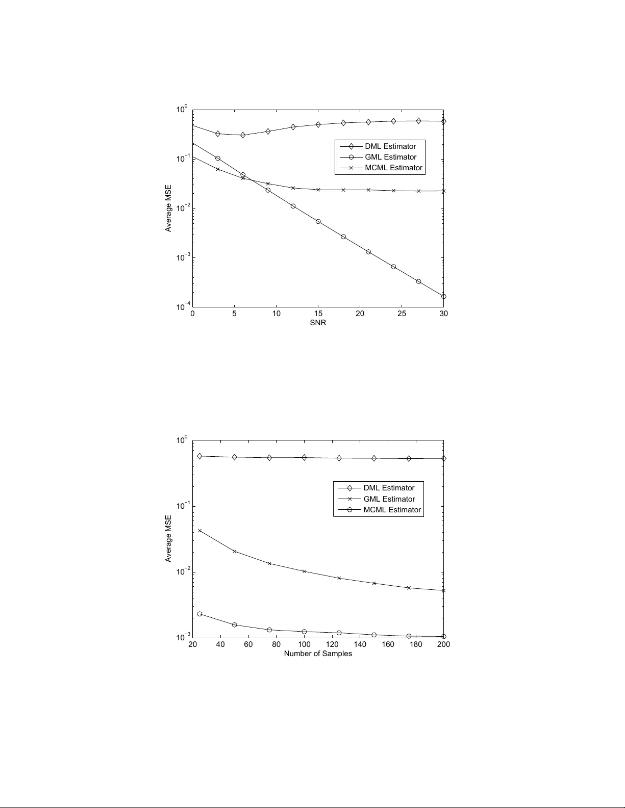
1 Blind Channel Estimation for Amplify-and-F orward T wo-W ay Relay Networks Emplo ying M -PSK Modulation Saeed Abdallah and Ioannis N. Psaromiligkos Abstract W e consider the problem of channel estimation for amplify-and-forward (AF) two-way relay networks (TWRNs). Most works on this problem focus on pilot-based approaches which impose a significant training ov erhead that reduces the spectral ef ficiency of the system. T o avoid such losses, this work proposes blind channel estimation algorithms for AF TWRNs that employ constant-modulus (CM) signaling. Our main algorithm is based on the deterministic maximum likelihood (DML) approach. Assuming M -PSK modulation, we show that the resulting estimator is consistent and approaches the true channel with high probability at high SNR for modulation orders higher than 2. For BPSK, howe ver , the DML performs poorly and we propose an alternativ e algorithm that performs much better by taking into account the BPSK structure of the data symbols. For comparati ve purposes, we also in vestig ate the Gaussian maximum-likelihood (GML) approach which treats the data symbols as Gaussian-distributed nuisance parameters. W e deri ve the Cramer -Rao bound and use Monte-Carlo simulations to in vestig ate the mean squared error (MSE) performance of the proposed algorithms. W e also compare the symbol-error rate (SER) performance of the DML algorithm with that of the training-based least-squares (LS) algorithm and demonstrate that the DML of fers a superior tradeof f between accurac y and spectral efficienc y . Index T erms : Amplify and F orward, Channel Estimation, Constant Modulus, Cramer-Rao bound, Maximum-likelihood, T wo-way Relays. The authors are with McGill University , Department of Electrical and Computer Engineering, 3480 University Street, Montreal, Quebec, H3A 2A7, Canada. Email: saeed.abdallah@mail.mcgill.ca; yannis@ece.mcgill.ca, phone: +1 (514) 398-2465, fax: +1 (514) 398-4470. This work was supported in part by the Natural Sciences and Engineering Research Council of Canada (NSERC) under grant 262017. This work was presented in part at the 2011 IEEE International Conference on Acoustics, Speech and Signal Processing (ICASSP), Prague, Czech Republic October 23, 2018 DRAFT 2 I . I N T R O D U C T I O N Amplify-and-forward (AF) two-way relay networks (TWRNs) [1] have recently emerged as a spectrally ef ficient approach for bidirectional communication between two terminals. The majority of works on TWRNs assume the av ailability of channel kno wledge at the terminals, which makes it important to de velop ef ficient channel estimation algorithms. Although some recent works ha ve considered noncoherent two-way relaying which a v oids channel estimation by employing dif ferential modulation schemes (c.f. [2], [3]), the resulting systems hav e lower performance than those employing coherent schemes. So far , researchers ha ve taken a training-based approach to channel estimation for AF TWRNs, estimating the channels using pilot symbols known to both terminals. In [4], the training-based maximum- likelihood (ML) estimator was dev eloped for the classical single-antenna single-relay system assuming flat-fading channels. In [5], the ML approach was used to acquire initial channel estimates at the relay that were employed to denoise the training signal. Power was then allocated at the relay to optimize channel estimation at the terminals. The case when the relay and the two terminals are equipped with multiple antennas was considered in [6], where initial estimates of the multi-input multi-output (MIMO) channels were acquired at each terminal using the training-based least-squares (LS) algorithm, and then a tensor -based approach was employed to improv e the estimation accuracy by exploiting the structure of the channel matrices. Channel estimation for TWRNs in frequenc y selecti ve environments has also been considered in a number of works. LS estimation for OFDM systems was considered in [7]. A nulling-based LS algorithm was proposed in [8] to jointly estimate the channel and the carrier -frequency of fset (CFO). Finally , channel estimation and the design of training symbols for TWRNs operating in time-v arying environments has been considered in [9], where a complex-exponential basis expansion model (CE-BEM) was used to facilitate LS channel estimation. The obvious shortcoming of the pilot-based approach is the training o verhead which in turn reduces the spectral efficienc y of TWRNs. Blind channel estimation would av oid this burden, which makes it a more spectrally-ef ficient approach. Little effort, ho wev er , has so far been dedicated to de velop blind channel estimation algorithms for TWRNs. In [10], a blind channel estimator was proposed for OFDM-based TWRNs by using the second-order statistics of the recei ved signal and applying linear precoding at both terminals, while in [11] a semi-blind approach to joint channel estimation and detection for MIMO- OFDM TWRNs was de veloped using the expectation conditional maximization (ECM) algorithm. In this work, we consider blind channel estimation for TWRNs that employ constant-modulus (CM) signaling. Because of its constant env elope, CM signaling permits the use of inexpensi ve and ener gy- October 23, 2018 DRAFT 3 ef ficient nonlinear amplifiers. In fact, CM signaling in the form of continuous-phase modulation (CPM) is employed in the well-known GSM cellular standard, while 8-PSK modulation is employed in the Enhanced Data Rates for GSM Evolution (EDGE) [12]. Moreover , QPSK modulation is supported in the 3rd Generation Partnership Program (3GPP) Long T erm Evolution (L TE) and L TE-Adv anced wireless standards [13]. CM signaling has also been employed in a number of works on amplify-and-forward relay networks [14]–[17]. In fact, a nov el relaying protocol has been recently proposed in [18] whereby CM signalling is employed both at the terminals and at the relay which only forwards the phase of the recei ved signal to the destination. This protocol is referred to as phase-only forward relaying. Assuming nonreciprocal flat-fading channels, we propose a deterministic ML (DML)-based algorithm that estimates the channel blindly by treating the data symbols as deterministic unkno wns. While the proposed algorithm may be applied to any type of CM signaling, we analyze its asymptotic performance assuming that the terminals employ M -PSK modulation. Noting that consistency is not guaranteed for ML estimators when the data symbols are treated as deterministic unkno wns [19], [20], we prove that our DML estimator is consistent when the channel parameters belong to compact sets. W e also study the asymptotic behavior of the DML estimator at high SNR and prov e that it approaches the true channel with high probability for modulation orders higher than 2. F or M = 2 , ho wev er , the DML estimator performs poorly , and we propose an alternati ve estimator based on the constrained ML (CML) approach which provides much better performance by explicitly taking into account the BPSK structure of the data symbols. As a simple alternati ve to the DML approach, we also consider the Gaussian ML (GML) estimator which can be obtained by treating the data symbols as Gaussian-distributed nuisance parameters. When CM signaling is employed, the GML estimator takes the form of a sample average which is consistent and can be updated online but suf fers from an error floor at high SNR. T o e v aluate the performance of our estimator , we also derive two Cramer-Rao bounds (CRBs) for our estimation problem. The first bound is obtained by treating the data symbols as deterministic unknown parameters and the second is the modified CRB [21] which treats the data symbols as random nuisance parameters. Monte Carlo simulations are used to in vestigate the performance of the proposed algorithms. For M > 2 , we show that the DML estimator outperforms the GML estimator at medium-to-high SNR and approaches the CRB at high SNR. For M = 2 we sho w that the CML-inspired estimator outperforms the GML estimator except at very lo w SNR. W e also in vestigate the tradeof fs of follo wing the blind approach by comparing the symbol-error rate (SER) performance of the DML estimator with that of the training-based LS estimator . W e show that the DML approach provides a better tradeoff between accuracy and spectral ef ficiency . October 23, 2018 DRAFT 4 The remainder of the paper is or ganized as follows. In Section II, we present our system model. In Section III we present the proposed algorithms. In Section IV, we analyze the asymptotic behavior of our estimators and derive the CRB. W e show our simulation results and comparisons in Section V. Finally , our conclusions are presented in Section VI. Fig. 1. The two-way relay network with two source terminals and one relay node. I I . S Y S T E M M O D E L W e consider the typical half-duplex TWRN with two source nodes, T 1 and T 2 , and a single relaying node R , sho wn in Fig. 1. The network operates in quasi-static flat-fading channel conditions. Each data transmission period is divided into two phases. In the first phase, T 1 and T 2 simultaneously transmit to R the M -PSK data symbols t 1 and t 2 , respecti vely . The symbols t 1 and t 2 are of the form t 1 = √ P 1 e φ 1 and t 2 = √ P 2 e φ 2 , where P 1 and P 2 are the transmission powers of T 1 , T 2 , respectiv ely , φ 1 and φ 2 are the information-bearing phases randomly and independently chosen from the set S M = { (2 ` − 1) π/ M , ` = 1 , . . . , M } , and  , √ − 1 . The recei ved signal at the relay during the first transmission phase is giv en by r = h 1 t 1 + g 1 t 2 + n, (1) where h 1 and g 1 are the complex coefficients of the flat-fading channels T 1 → R and T 2 → R , respecti vely , and n is zero-mean complex additiv e white Gaussian noise (A WGN) with v ariance σ 2 r . In the second phase, R broadcasts the amplified signal Ar , where A is the amplification factor , assumed to be known at both terminals as is common practice (cf. [4], [5]). The amplified signal passes through the channels h 2 and g 2 to reach T 1 and T 2 , respectiv ely . The complex channel coefficients h 1 , h 2 , g 1 and g 2 remain fixed during the estimation period. T o maintain an av erage power of P r at the relay o ver the long term, the amplification factor is chosen as [4] A = s P r P 1 + P 2 + σ 2 r . (2) October 23, 2018 DRAFT 5 W ithout loss of generality , we consider channel estimation at node T 1 . The recei ved signal at T 1 in the second transmission phase is z = Ah 1 h 2 t 1 + Ag 1 h 2 t 2 + Ah 2 n + η , (3) where η is the zero-mean A WGN term at T 1 with v ariance σ 2 t . W e assume that the noise v ariances σ 2 r and σ 2 t are unkno wn at T 1 . The term Ah 1 h 2 t 1 represents the self-interference at T 1 . In (3), there are 6 unkno wn real channel parameters: the magnitudes and phases of the complex parameters h 1 , h 2 , and g 1 . Ho wev er , not all of them are identifiable. By inspecting (3), we see that the channel parameters which can be identified (blindly or otherwise) when the noise variances are unknown are 1 | h 1 || h 2 | , | g 1 || h 2 | , ∠ h 1 + ∠ h 2 , and ∠ g 1 + ∠ h 2 . On the other hand, it is not possible to identify the individual magnitudes | h 1 | , | h 2 | and | g 1 | , or individual phases ∠ h 1 , ∠ h 2 and ∠ g 1 . In other words, the identifiable channel parameters are a , h 1 h 2 and b , g 1 h 2 . Under the CM assumption, it is suf ficient for detection purposes to kno w a and φ b , ∠ b . I I I . P R O P O S E D C H A N N E L E S T I M A T I O N A L G O R I T H M S Estimation is performed at T 1 using N receiv ed samples, z i , i = 1 , . . . , N , of the form gi ven by (3). The time index i , i = 1 , . . . , N , is used to indicate the realizations of t 1 , t 2 , φ 1 , φ 2 , n , η , that ga ve rise to each sample z i . Let 2 z , [ z 1 , . . . , z N ] T be the vector of received samples. This vector can be expanded as z = Aa t 1 + Ab t 2 + Ah 2 n + η , (4) where t 1 , [ t 11 , . . . , t 1 N ] T , t 2 , [ t 21 , . . . , t 2 N ] T , n , [ n 1 , . . . , n N ] T and η , [ η 1 , . . . , η N ] T . A. Deterministic ML Appr oach T o av oid dealing with a complicated likelihood function, we treat the transmitted symbols t 2 i , i = 1 , . . . , N as deterministic unkno wns. W e also ignore the finite alphabet constraint that restricts the phases φ 2 i , i = 1 . . . , N to the set S M . Nonetheless, the actual statistics of these phases will be used in Section IV to analyze the beha vior of the resulting estimator . Due to the abo ve assumptions, the DML approach can be used to blindly estimate the sums φ bi , φ 2 i + φ b , i = 1 , . . . , N , but it cannot be used to obtain separate estimates of φ b and φ 2 i , i = 1 . . . , N . Ho we ver , since M -PSK modulation is assumed, the V iterbi-V iterbi 1 In this paper , | · | and ∠ ( · ) denote the magnitude and phase of a complex number, respectiv ely . 2 In this paper , ( · ) T and ( · ) ∗ are used to denote the transpose and complex conjugate operations, respectiv ely . October 23, 2018 DRAFT 6 algorithm [22] may be used to blindly estimate φ b . A fe w pilots, ho we ver , are still needed to resolv e the resulting M -fold ambiguity in φ b . W e define the vector of unknown parameters for the DML algorithm as θ , [ a, | b | , φ b 1 , . . . , φ bN , σ 2 o ] T , where σ 2 o , A 2 | h 2 | 2 σ 2 r + σ 2 t is the overall noise v ariance at T 1 . W ith t 2 assumed deterministic and t 1 kno wn, the received vector z is complex Gaussian with E { z } = Aa t 1 + Ab t 2 and co variance E { z z H } = σ 2 o I . Hence, the log-likelihood function is giv en by L ( z ; θ ) = − 1 σ 2 o k z − Aa t 1 − Ab t 2 k 2 − N log  π σ 2 o  = − 1 σ 2 o N X i =1    z i − Aat 1 i − A | b | p P 2 e φ bi    2 − N log  π σ 2 o  . (5) Let ˆ a , b | b | , c σ 2 o , ˆ φ bi be the ML estimates of a , | b | , σ 2 o and φ bi , i = 1 , . . . , N , respectively . It is straightforward to show that ˆ φ bi = ∠ ( z i − A ˆ at 1 i ) , which when substituted into L ( z ; θ ) yields the updated log-likelihood L 0 ( z ; a, | b | , σ 2 o ) = − 1 σ 2 o N X i =1  | z i − Aat 1 i | − A | b | p P 2  2 − N log  π σ 2 o  . (6) Maximizing (6) with respect to | b | , we get b | b | = N P i =1 | z i − A ˆ at 1 i | N A √ P 2 . (7) Substituting b | b | in place of | b | in (6), we obtain L 00 ( z ; a, σ 2 o ) = − 1 σ 2 o N X i =1 | z i − Aat 1 i | − 1 N N X k =1 | z k − Aat 1 k | ! 2 − N log  π σ 2 o  . (8) Hence, the ML estimate of a is giv en by 3 ˆ a = arg min u ∈ C ( N X i =1 | z i − Aut 1 i | − 1 N N X k =1 | z k − Aut 1 k | ! 2 ) . (9) Finally , the ML estimate of the parameter σ 2 o is neither needed for detection nor for estimating a , | b | , 3 W e note that a slightly dif ferent estimator may be obtained by using a likelihood function that also takes into account the pilot symbols used to resolv e the ambiguity in φ b . Since the required number of pilots is very small, the resulting estimator will only be slightly better than (9). October 23, 2018 DRAFT 7 but is pro vided for completeness and is giv en by c σ 2 o = 1 N N X i =1 | z i − A ˆ at 1 i | − 1 N N X k =1 | z k − A ˆ at 1 k | ! 2 . (10) W e note that the parameter | b | is also not needed for detection when CM signaling is used. The ML estimator in (9) has an intuitive interpretation. Let ˜ z i ( u ) , z i − Aut 1 i , i = 1 , . . . , N be the “cleaned” versions of the receiv ed signal samples after self-interference has been remov ed using the complex value u as an estimate of a . The signals ˜ z i ( u ) , i = 1 , . . . , N are independently-generated realizations of the R V ˜ z ( u ) , A ( a − u ) t 1 + Abt 2 + Ah 2 n + η . The quantity W N ( u ) = 1 N − 1 N X i =1 | ˜ z i ( u ) | − 1 N N X k =1 | ˜ z k ( u ) | ! 2 (11) which is the objective function in (9), scaled by 1 N − 1 , also represents the sample-v ariance of the en velope of ˜ z ( u ) . W e demonstrate in Section IV that the value u = a which completely cancels the interference also minimizes the variance of the en velope of ˜ z ( u ) . Hence, the v ariance of the en velope of ˜ z ( u ) may be seen as a measure of the lev el of self-interference. By treating the transmitted symbols t 2 i , i = 1 , . . . , N as deterministic unknowns, the estimator in (9) ignores the underlying structure of the phases φ 2 i , i = 1 , . . . , N . A valid question is whether a better blind estimator may be obtained by explicitly taking into account the structure of the phases. This question is particularly rele v ant for BPSK modulation, for which we show in Section IV that the DML estimator in (9) performs poorly as it experiences infinitely man y global minima at high SNR. There are two alternati ve blind ML approaches which take into account the phase structure of the data. The first approach is to perform ML estimation using the likelihood function f ( z | a, b, σ 2 o ) which can be obtained by treating t 2 i , i = 1 , . . . , N as random parameters and marginalizing ov er them. Unfortunately , this approach is very complicated due to the mix ed-Gaussian nature of f ( z | a, b, σ 2 o ) . The other alternati ve is to follow a constrained ML (CML) approach by solving the likelihood function in (5) subject to the constraint that φ 2 i ∈ S M , i = 1 , . . . , N . For higher order modulations, it is difficult to apply this approach and still obtain a closed-form objective function. Ho we ver , as we shall see ne xt, this approach becomes more feasible for BPSK modulation. B. Constrained ML Appr oach for BPSK As we will see shortly , a straightforward application of the CML approach for M = 2 is not feasible as it results in a 3-dimensional search. Ho we ver , it is possible to obtain a CML-inspired estimator which October 23, 2018 DRAFT 8 possesses a closed-form objectiv e function by utilizing just a fe w pilot symbols to estimate the phase φ b . Under BPSK modulation, the CML approach minimizes the same log-lik elihood function as in (5), but subject to the constraint that t 2 i = ± √ P 2 , i = 1 , . . . , N . W e focus on the first term in (5) since the estimation of σ 2 o is decoupled from the estimation of the remaining parameters. Let J ( z ; a, | b | , φ b , t 2 ) , N X i =1    z i − Aat 1 i − A | b | p P 2 e  ( φ bi )    2 (12) be our objectiv e function. The resulting estimate of t 2 i , i = 1 , . . . , N , is ˆ t 2 i = p P 2 sgn  <{ e − φ b ( z i − Aat 1 i ) }  . (13) Substituting (13) back into (12), we obtain J 0 ( z ; a, | b | , φ b ) = N X i =1 | z i − Aat 1 i | 2 + N A 2 | b | 2 P 2 − 2 A | b | p P 2 N X i =1 |<{ e − φ b ( z i − Aat 1 i ) }| . (14) From (14), we see that the CML estimate of | b | is given by b | b | c = 1 N A √ P 2 N X i =1 |<{ e − φ b ( z i − Aat 1 i ) }| . (15) Substituting (15) into (14), we obtain the updated objectiv e function J 00 ( z ; a, φ b ) = N X i =1 | z i − Aat 1 i | 2 − 1 N N X i =1 |<{ e − φ b ( z i − Aat 1 i ) }| ! 2 (16) which we hav e to solve for a and φ b . The CML estimate of φ b in terms of a is the solution of the follo wing maximization problem ˆ φ bc = arg max ψ ∈ [0 , 2 π ) N X i =1 | z i − Aat 1 i || cos( ∠ ( z i − Aat 1 i ) − ψ ) | . (17) Unfortunately , the maximization in (17) does not have a closed-form solution, which means that we cannot proceed to obtain an objectiv e function that only depends on a , lik e the one in (9). Thus, a strict application of the CML approach requires the use of a 3-dimensional search to estimate a and φ b . T o get around this problem, we propose to replace φ b in (16) with a pilot-based estimate of φ b and then proceed to estimate a . W e let x 1 j , x 2 j and s j , j = 1 , . . . , J, be the J pilot symbols transmitted by T 1 and T 2 and the corresponding samples received at T 1 , respecti vely . W e may thus estimate φ b by October 23, 2018 DRAFT 9 ˆ φ b = ∠ J P j =1 ( s j − Aax 1 j ) x 2 j . Substituting ˆ φ b into (16), we obtain the following estimate of a ˆ a c = arg min u ∈ C N X i =1 | z i − Aut 1 i | 2 − 1 N   N X k =1       <    ( z k − Aut 1 k ) e −  ∠ J P j =1 ( s j − Aux 1 j ) x 2 j            2 . (18) W e refer to the estimator in (18) as the modified CML (MCML) estimator . C. Gaussian ML Appr oach In deriving the DML and the MCML estimators, we treated the data symbols t 2 i , i = 1 , . . . , N as deterministic unkno wns. Another approach commonly used to deal with nuisance parameters is Gaussian ML estimation [23]. In this case, the data symbols t 2 i , i = 1 , . . . , N are treated as i.i.d. complex Gaussian random v ariables with mean zero and v ariance P 2 . Under this assumption, the total noise variance becomes σ 2 g , P 2 | b | 2 + σ 2 o . The resulting log-likelihood function on a is L ( z ; a ) = − 1 σ 2 g k z − Aa t 1 k 2 − N log( π σ 2 g ) . (19) Hence, the GML estimate of a is ˆ a g = N P i =1 t ∗ 1 i z i N P i =1 | t 1 i | 2 = 1 N AP 1 N X i =1 t ∗ 1 i z i . (20) Thus, the GML estimate of a has the form of a computationally inexpensi ve sample-av erage. It can be easily updated at run-time by updating the a verage term as ne w samples arrive. The GML estimator will serve as a low-comple xity benchmark with which to compare the performance of the proposed DML and MCML estimators. I V . A S Y M P T OT I C B E H A V I O R A N A LY S I S In this section, we analyze theoretically the asymptotic behavior of the proposed estimators. Since the parameters | b | and σ 2 o are not required for detection, our analysis focuses on the estimation of a . Regarding the DML estimator , the fact that we treat the phases φ bi , i = 1 , . . . , N as deterministic unknowns means that the number of real unknown parameters for N (complex) samples is N + 4 . Because the dimension of the parameter space grows linearly with the number of samples, the DML estimator falls within a special class of ML estimators that are based on “partially-consistent observ ations” [19]. The estimated parameters can be classified into two groups. The first group are the incidental parameters φ bi , i = 1 , . . . , N . Each October 23, 2018 DRAFT 10 incidental parameter af fects only a finite number of samples (a single sample in our case). The other group of parameters, a , | b | , and σ 2 o , affect all recei ved samples and are thus called structural parameters. The estimation of structural parameters in the presence of incidental parameters has been in vestigated in the literature [19], [20], [24], [25] and is referred to as the Incidental Parameter Problem. It is well-known that the asymptotic properties of ML estimators, such as consistency , which hold when the dimension of the parameter space is fixed do not necessarily hold in the presence of incidental parameters [19]. It thus becomes important to inv estigate the asymptotic behavior of the DML estimator . W e do this by e xplicitly taking into account the fact that φ 1 i and φ 2 i , i = 1 , . . . , N are equiprobably and independently chosen from the set S M . Re garding the powers P 1 , P 2 and P r , the most common con v ention in TWRNs is to set P 1 = P 2 = P r (cf. [5], [7], [26]), e ven though some w orks use slightly dif ferent setups. F or instance, the authors in [4] choose P 2 = 2 P 1 and P r = 1 2 ( P 1 + P 2 ) . In our analysis we consider the general case of P 1 = αP 2 and P r = β ( P 1 + P 2 ) for some α, β > 0 . The first asymptotic property we address is the consistenc y of the DML estimator , which we prov e to hold when the parameter spaces of a and b are restricted to compact sets. This is true even for BPSK modulation. The second aspect we address is ho w the DML estimator beha ves at high SNR (we will define SNR shortly). W e show the estimator approaches the true channel with high probability at high SNR for M > 2 , while it encounters infinitely-man y global minima at high SNR for M = 2 . W e also analyze the high SNR behavior of the MCML estimator , sho wing that it approaches the true channel with high probability for J = 1 (single pilot). For J > 1 , the pilots can be chosen such that the MCML estimator always approaches the true channel at high SNR. A. Consistency of the DML Estimator In this section, we study the behavior of the DML estimator as N → ∞ . W e demonstrate that the DML estimator is consistent when the channel parameters a , b belong to compact sets. This holds for any M ≥ 2 and for any P 1 , P 2 , σ 2 r , σ 2 t . Before proceeding, we note that the estimator of a in (9) belongs to the class of extremum estimators. An estimator ˆ ω is called an extremum estimator (cf. [27], [28]) if there is an objectiv e function Σ N ( ω ) such that ˆ ω = arg min ω ∈ Ω Σ N ( ω ) , where Ω is the set of parameter v alues. The fundamental theorem for the consistency of e xtremum estimators can be summarized as follows: Theoem 1 (Newey and McFadden [28, Ch. 36, Theorem 2.1]). If ω belongs to a compact set Ω and Σ N ( ω ) con ver ges uniformly in pr obability to Σ o ( ω ) as N → ∞ , wher e Σ o ( ω ) is continuous and uniquely October 23, 2018 DRAFT 11 minimized at ω = ω o , then ˆ ω con ver ges in pr obability to ω o . Thus, we need to establish that, as N → ∞ , the objectiv e function W N ( u ) in (11) con v erges uniformly in probability to a deterministic function of u which has a unique global minimum at u = a . Letting v , a − u , and V N ( v ) , W N ( a − v ) , we obtain V N ( v ) = 1 N − 1 N X i =1 | y i ( v ) | − 1 N N X k =1 | y k ( v ) | ! 2 , (21) where y i ( v ) , ˜ z i ( a − v ) . The terms y i ( v ) , i = 1 , . . . , N are independently-generated realizations of the R V y ( v ) , ˜ z ( a − v ) , and V N ( v ) is the sample v ariance of the en v elope of y ( v ) . Let V ( v ) be the variance of | y ( v ) | , ϕ k , 2 π k M , and θ k ( v ) , φ v − φ b + ϕ k for k = 0 , . . . , M − 1 . W e sho w in Appendix A that V ( v ) = A 2 | v | 2 P 1 + A 2 | b | 2 P 2 + σ 2 o − r π σ 2 o 4 M 2 M − 1 X k =0 L 1 / 2 ( − λ k ( v )) ! 2 , (22) where L 1 / 2 ( · ) is the Laguerre polynomial [29] with parameter 1 / 2 , and λ k ( v ) = 1 σ 2 o  A 2 | v | 2 P 1 + A 2 | b | 2 P 2 + 2 A 2 | v || b | p P 1 P 2 cos( θ k ( v ))  . (23) The behavior of V ( v ) for v = 0 , which corresponds to u = a , is described in the following lemma: Lemma 1. The variance V ( v ) of the r andom variable | y ( v ) | has a unique global minimum occurring at v = 0 . Pr oof: See Appendix B. T o apply Theorem 1, it remains to establish that V N ( v ) con ver ges uniformly in probability to V ( v ) . Since V N ( v ) is the sample variance of | y ( v ) | and | y ( v ) | has a finite fourth central moment, V N ( v ) con ver ges in probability to V ( v ) [30]. The following lemma holds regarding uniform con v ergence in probability which is a stricter requirement than con ver gence in probability: Lemma 2. Suppose a , b and v all belong to compact sets, then V N ( v ) con ver ges uniformly in pr obability to V ( v ) . Pr oof: See Appendix C. From Lemma 1 and Lemma 2, we see that all of the conditions of Theorem 1 are met if the channel parameters a and b belong to compact sets. Hence, the following theorem holds. Theorem 2. If the channel parameter s a , b belong to the compact sets B 1 and B 2 , then the following October 23, 2018 DRAFT 12 estimator of a ˆ a = arg min u ∈ B 1 ( N X i =1 | z i − Aut 1 i | − 1 N N X k =1 | z k − Aut 1 k | ! 2 ) . is consistent. The compactness assumption for a and b can be satisfied by assuming that the magnitudes of g 1 , h 1 and h 2 are bounded. If we treat g 1 , h 1 and h 2 as complex Gaussian random v ariables, there is no upper bound on | a | and | b | , strictly speaking, but we can always choose a suf ficiently large ξ such that P r ob ( | a | , | b | ≤ ξ ) = 1 −  , where  can be made arbitrarily small. B. High SNR Behavior of the DML Estimator W e no w in vestigate the behavior of the DML estimator at high transmit SNR. T o simplify our presentation, we assume that σ 2 r = σ 2 t = σ 2 . This assumption allows for a simple and intuiti v e definition of SNR as γ , P 2 σ 2 . Let X ( v ) = N X i =1 | Av t 1 i + Abt 2 i | − 1 N N X k =1 | Av t 1 k + Abt 2 k | ! 2 (24) be the objective funcion in (9) in the limit as σ → 0 . The follo wing lemma describes the beha vior of the DML estimator as σ → 0 . Lemma 3. F or fixed (finite) N , the DML estimator appr oaches the true channel a as σ → 0 , except when the data symbols ar e such that the phase differ ences φ 1 i − φ 2 i , i = 1 , . . . , N take at most two distinct values, in whic h case the objective function encounters infinitely many global minima as σ → 0 . Ther efor e, assuming M -PSK transmission, ˆ a → a as σ → 0 with pr obability P M , N = 1 −  2 M  N − 1 ( M − 1) . Pr oof: See Appendix D. As we can see from Lemma 3, the DML estimator approaches the true channel except in the ev ent that the phase dif ferences φ 1 i − φ 2 i , i = 1 , . . . , N happen to take at most two distinct v alues. When this ev ent occurs, the objecti ve function of the estimator will hav e infinitely man y global minima at high SNR. In fact, the occurence of this ev ent also results in a singular Fisher information matrix as we shall see in Section IV -E. For M > 2 , this ev ent is highly unlikely for sufficiently large N . For instance, at M = 4 , the probability of this event is less than 5 . 6 × 10 − 9 for N ≥ 30 . Thus, the DML estimator approaches the true channel with high probability for M > 2 as long as the sample size is not extremely small. In this case, the a verage MSE performance of the estimator keeps impro ving with SNR, and it October 23, 2018 DRAFT 13 can ef fectiv ely achie ve arbitrary accurac y for sufficiently high SNR. For M = 2 , ho we ver , P 2 , N = 0 and the estimator alw ays encounters infinitely-many global minima at high SNR because the dif ference φ 1 i − φ 2 i cannot take more than two distinct v alues for i = 1 , . . . , N . In fact, for M = 2 and for any non-zero v , b, there are only two possible values that the terms | v t 1 i + bt 2 i | , i = 1 , . . . , N can take, and they are | √ P 1 v + √ P 2 b | and | √ P 1 v − √ P 2 b | . Whene ver 4 v ⊥ b , these two values are equal, which means that the terms | v t 1 i + bt 2 i | , i = 1 , . . . , N are all equal regardless of the values of t 1 i , t 2 i , i = 1 , . . . , N . Therefore, all the values of v such that v ⊥ b are global minimizers of the objecti ve function X ( v ) , and the estimator is not able to identify the true channel. Hence, the DML estimator performs poorly for M = 2 as its MSE performance degrades at high SNR. Despite this behavior , the DML estimator is consistent for M = 2 for any fixed σ > 0 , because for σ > 0 only v = 0 minimizes the v ariance V ( v ) . This explains why , as we shall see, the DML estimator performs better at low SNR than high SNR for M = 2 . Since the performance of the estimator will also degrade for very lo w SNR, the MSE for M = 2 exhibits a U-shaped behavior when plotted versus SNR. This is confirmed by our simulation results in Section V. W e note that similar high SNR behavior is encountered if the noise v ariances σ 2 r and σ 2 t are assumed to be different (b ut fixed) and the transmit po wer P 2 becomes asymptotically high. C. High SNR Behavior of the MCML Estimator (M=2) W e now in vestigate the high SNR behavior of the MCML estimator and show that by taking into account the BPSK structure of the data symbols it effecti vely avoids the problem of infinitely many global minima at high SNR. Let Y ( v ) , N X i =1 | Av t 1 i + Abt 2 i | 2 − 1 N N X k =1 | Av t 1 k + Abt 2 k | · | cos(∆ k ) | ! 2 (25) be the objectiv e function in (18) as σ → 0 , e xpressed in terms of v = a − u , where ∆ k = ∠ ( Av t 1 k + Abt 2 k ) − ∠ ( J AbP 2 + Av J X j =1 x 1 j x 2 j ) . (26) Clearly , Y ( v ) ≥ 0 and Y (0) = 0 . It remains to in vestigate whether it is possible to have Y ( v ) = 0 for v 6 = 0 , i.e., whether there could be other global minima besides v = 0 . For this to happen, the terms | Av t 1 k + Abt 2 k | , k = 1 , . . . , N have to be all equal and the terms | cos(∆ k ) | , k = 1 , . . . , N have to be all 4 The notation x ⊥ y means that ∠ x − ∠ y = π 2 mod π . October 23, 2018 DRAFT 14 equal to 1 . The first requirement can be met if v ⊥ b or if the product t 1 i t 2 i is the same for i = 1 , . . . , N . As for the second requirement, it is only satisfied when ∠ ( Av t 1 k + Abt 2 k ) = ∠ ( J AbP 2 + Av J X j =1 x 1 j x 2 j ) mod π (27) for k = 1 , . . . , N , where mod is the modulo operator . Let H be the ev ent that the requirement in (27) is satisified for k = 1 , . . . , N . For J = 1 , H occurs with probability P ( H ) = 1 / 2 N . For J > 1 , ho wev er , the occurrence of H can be completely a v oided if the pilots are chosen such that the products x 1 j x 2 j , j = 1 , . . . , J are not all equal. If the pilots are randomly chosen, then P ( H ) = 1 / 2 N + J − 1 . Hence, depending on the choice of the pilots, the MCML estimator either always approaches the true channel or approaches it with a probability of 1 − 1 / 2 N + J − 1 . Thus, the MCML estimator ef fecti vely resolves the problem of infinitely many global minima at high SNR e ven when a single pilot is used. D. MSE P erformance of the GML Estimator The estimator of a in (20) can be expanded as ˆ a g = a + b N √ α N X i =1 e  ( φ 2 i − φ 1 i ) + 1 N √ αP 2 N X i =1 e − j φ 1 i h 2 n i + 1 N A √ αP 2 N X i =1 e − j φ 1 i η i . (28) It is straightforward to check that the estimator is unbiased. The resulting MSE is E {| ˆ a g − a | 2 } = | b | 2 N α + | h 2 | 2 σ 2 N αP 2 + σ 2 N A 2 αP 2 . (29) Since E {| ˆ a g − a | 2 } → 0 as N → ∞ , the estimator is consistent. Clearly , as σ → 0 , the MSE performance of this estimator is limited by an error floor of | b | 2 N α . E. Cramer-Rao Bounds In this section, we obtain CRBs for the estimation of a and | b | . The first bound is the standard CRB deri ved by treating the data symbols t 21 , . . . , t 2 N as deterministic unknowns. W e exclude the parameter σ 2 o from our CRB deriv ation since its Fisher information is decoupled from the Fisher information of the other parameters. Let θ R , [ <{ a } , ={ a } , | b | , φ b 1 , . . . , φ bN ] T be the vector of real unkno wn parameters (excluding σ 2 o ), and let I ( θ R ) be the corresponding Fisher information matrix (FIM). The matrix I ( θ R ) is gi ven by I ( θ R ) =   H 1 H 2 H T 2 H 3   , (30) October 23, 2018 DRAFT 15 where H 1 = 1 σ 2 o      2 A 2 N P 1 0 2 A 2 <{ e φ b t H 1 t 2 } 0 2 A 2 N P 1 2 A 2 ={ e φ b t H 1 t 2 } 2 A 2 <{ e φ b t H 1 t 2 } 2 A 2 ={ e φ b t H 1 t 2 } 2 A 2 N P 2      , (31) H 2 = 1 σ 2 o      2 A 2 ={ b ∗ t 11 t ∗ 21 } . . . 2 A 2 ={ b ∗ t 1 N t ∗ 2 N } 2 A 2 <{ b ∗ t 11 t ∗ 21 } . . . 2 A 2 <{ b ∗ t 1 N t ∗ 2 N } 0 . . . 0      , (32) and H 3 = 1 σ 2 o 2 A 2 | b | 2 P 2 I N . (33) The resulting CRBs on the estimation of a and | b | are 5 C RB a = [ I − 1 ( θ R )] 11 + [ I − 1 ( θ R )] 22 , (34) and C RB | b | = [ I − 1 ( θ R )] 33 . (35) Moreov er , using the Schur-complement property and letting ˜ H , H 1 − H 2 H − 1 3 H T 2 , we obtain 6 C RB a = [ ˜ H − 1 ] 11 + [ ˜ H − 1 ] 22 , (36) and C RB | b | = [ ˜ H − 1 ] 33 . (37) The bounds C RB a and C RB | b | exist whenev er ˜ H is in vertible. It can be sho wn that det ( ˜ H ) = 0 whene ver the data symbols are such that the differences φ 1 i − φ 2 i , i = 1 , . . . , N take at most two distinct v alues, (recall that this is the same condition which results in infinitely many global minima at high SNR). Hence, the bounds do not exist for BPSK modulation since this condition is always met for M = 2 . The bounds C RB a and C RB | b | are both functions of t 1 and t 2 , and thus the y hold for the particular realizations of t 1 and t 2 under consideration. In Section V, we use Monte-Carlo simulations to av erage C RB a and C RB | b | ov er many realizations of t 1 and t 2 . 5 The notation [ A ] ij is used to refer to the ( i, j ) th element of the matrix A . 6 Although it is possible to ev aluate the expressions in (36) and (37) and obtain closed-form expressions for C RB a amd C R B | b | , the resulting e xpressions are quite lengthy , and are omitted for the sake of brevity . October 23, 2018 DRAFT 16 Another v ariant of the CRB, commonly used in the presence of random nuisance parameters is the Modified CRB (MCRB) [21]. In deriving the MCRB, we compute a modified FIM (MFIM) by first extracting the submatrix of the con v entional FIM which corresponds only to the nonrandom parameters ( <{ a } , ={ a } and | b | ) and then obtaining the expectation of this submatrix with respect to the random nuisance parameters ( t 2 in our case). Let θ 0 , [ <{ a } , ={ a } , | b | ] T , the MFIM is I m ( θ 0 ) , E { H 1 } = 1 σ 2 o      A 2 N P 1 0 0 0 2 A 2 N P 1 0 0 0 2 A 2 N P 2      . (38) Hence, M C RB a = σ 2 o A 2 N P 1 and M C RB | b | = σ 2 o 2 A 2 N P 2 . (39) The bounds in (39) ha ve the adv antage of possessing a simple closed form. Howe v er , they are not as tight as the standard CRB and for this reason we will only use the bounds in (36) and (37) in our simulation results. V . S I M U L AT I O N R E S U LT S In this section, we use Monte-Carlo simulations to numerically inv estigate the performance of the proposed algorithms. Our results are obtained assuming P r = P 1 = P 2 , and they are av eraged using a set of 300 independent realizations of the channel parameters h 1 , h 2 , g 1 and g 2 . These realizations are generated by treating h 1 and h 2 as correlated complex Gaussian random variables with mean zero, v ariance 1 a correlation coefficient % = 0 . 3 , and also treating g 1 and g 2 as correlated complex Gaussian random variables with the same mean, v ariance and correlation coef ficient, b ut independent of h 1 and h 2 . T o generate correlated complex Gaussian random v ariables we follo w the approach proposed in [31]. The ML and MCML estimates are obtained using a two-dimensional grid-search with a step-size of 10 − 3 . As before, the SNR is defined as γ = P 2 σ 2 . Unless otherwise mentioned, MSE results are for the estimation of a . W e begin by comparing the MSE performance of the DML, GML and MCML estimators for M = 2 . W e do not sho w the CRB in this case, since the FIM is singular . The MSE performance of the three estimators is plotted versus SNR for N = 45 in Fig. 2 and versus N for an SNR of 20 dB in Fig. 3. For the MCML estimator , 2 pilots are employed to obtain an estimate of φ b . Both plots show that the DML estimator performs poorly for BPSK modulation and is outperformed by the GML and MCML estimators. Fig. 2 shows the U-shaped behavior of the DML estimator for M = 2 described in Section IV -B. October 23, 2018 DRAFT 17 The MCML estimator is superior to the GML estimator except at very lo w SNR. Moreover , as SNR increases, the MCML estimator improves steadily while the GML estimator hits an error floor . Fig. 3 also demonstrates the superiority of the MCML estimator to the GML estimator . Next, we study the MSE performance of the DML and GML estimators for M = 4 (QPSK modulation). The MSE performance of the two estimators is plotted versus SNR for N = 45 in Fig. 4 and versus N for an SNR of 20 dB in Fig. 5. The bound C RB a is sho wn as a reference in both plots. As we can see in Fig. 4, the DML estimator outperforms the GML estimator , except at lo w SNR. Moreover , the MSE performance of the DML estimator improves steadily with SNR and approaches C R B a , while that of the GML estimator hits an error floor at high SNR. In Fig. 4, it is also noticed that the MSE of the GML estimator goes belo w C RB a at low SNR. This should not be a surprise since C RB a is deriv ed by treating t 2 as deterministic, and the GML estimator is biased in this case. As we can see in Fig. 5, both estimators improv e as N increases, but the DML estimator is much closer to C RB a . In Fig. 6, the MSE performance of the DML and the GML estimators for the estimation of | b | and the associated CRB are plotted versus SNR for M = 4 . F or the GML estimator , we obtain an estimate of | b | by substituting ˆ a g in (7). Fig. 6 shows that the GML estimator is slightly better except at high SNR where it appears to hit an error floor and the DML estimator becomes better and approaches C RB | b | . It must be noted that | b | plays no role in detection when M -PSK modulation is used. Our ne xt goal is to compare the SER performance of the DML estimator with that of the training- based LS estimator in order to in vestig ate the tradeof fs between accuracy and spectral efficienc y that result from follo wing the blind approach. W e focus on small sample sizes since this is more suitable for modern-day cellular systems. W e note that, when channels are nonreciprocal, the training-based LS estimator is an efficient estimator which coincides with the training-based ML estimator . As a reference, we also plot the SER performance under perfect channel knowledge. The phase φ b is estimated blindly using the V iterbi-V iterbi algorithm 7 , and a small number of pilots is employed to resolve the resulting M -fold ambiguity using the unique word method [32]. In Fig. 7, we sho w the SER performance of the two algorithms assuming that the channel is fixed for the duration of 20 samples. For the DML estimator , 2 pilots and 18 data symbols are transmitted. The 2 pilots are used to resolve the M -fold ambiguity , and all 20 samples are used to blindly estimate a . F or the LS estimator , we estimate a and b using 4 pilot 7 Using the V iterbi-V iterbi algorithm, we estimate φ b by ˆ φ b , 1 M ∠ P N i =1 | ˜ z i (ˆ a ) | 2 e M ∠ ˜ z i (ˆ a )+ π , where ˜ z i (ˆ a ) , i = 1 , . . . , N are the resulting N samples after the estimate ˆ a is used to remo ve self-interference. October 23, 2018 DRAFT 18 symbols 8 and we transmit 16 data symbols. As we can see from Fig. 7, the SER performance of the DML estimator is very close to that of the LS estimator (approximately 0.6 dB away). In Fig. 8, we assume that the channel is fixed for the duration of 40 samples. In the DML case 4 pilots and 36 data symbols are transmitted, and in the LS case 8 pilots and 32 data symbols are transmitted. The performance of DML estimator is again very close to that of the LS estimator (approximately 0.4 dB aw ay), and it is only 1 . 5 dB away from the performance under perfect CSI. In both examples, for the DML algorithm we use 90% of the channel coherence time to transmit data and 10% to transmit pilots, while for the LS algorithm we are use 80% of the coherence time to transmit data and 20% to transmit pilots, which demonstrates that the DML estimator offers a better tradeof f between accuracy and spectral ef ficiency . It is worth noting that the channel coherence times considered in our SER studies are compatible with current wideband cellular systems. F or instance, considering a wideband system with 256 carriers and a sampling frequency of 10 − 6 s, the channel has to be in v ariant for 5 . 12 ms in the first example and for 10 . 24 ms in the second example. Assuming a central frequenc y of 2 . 4 GHz and a v ehicle speed of 10 m/s, the coherence time is around 12 . 5 ms, which is lar ger than the required coherence time in both examples. V I . C O N C L U S I O N S In this work, we proposed the DML algorithm for blind channel estimation in AF TWRNs emplo ying M -PSK modulation. The DML estimator was deriv ed by treating the data symbols as deterministic unkno wns. For comparison, we deriv ed the GML estimator by treating the data symbols as Gaussian- distributed nuisance parameters. W e showed that the DML estimator is consistent. For M > 2 , we showed that it approaches the true channel with high probability as SNR increases and that its MSE performance is superior to that of the GML estimator for medium-to-high SNR and approaches the deri ved CRB at high SNR. In contrast, the GML estimator suffers from an error floor at high SNR. W e also compared the SER performance of the DML estimator with that of the training-based LS estimator and sho wed that the DML approach provides a better tradeoff between accurac y and spectral efficiency . For M = 2 , ho wev er , we sho wed that the DML estimator performs poorly and proposed the MCML estimator which explicitly takes into account the structure of the BPSK signal. This estimator outperforms the GML estimator except at v ery low SNR and approaches the true channel at high SNR. 8 For the training-based LS algorithm, the pilots are chosen such that the pilot vectors from the two terminals are orthogonal to each other . October 23, 2018 DRAFT 19 Acknowledgments The authors of this work would like to thank Mr . Ali Shahrad for his help in pro ving Theorem 2 and the Associate Editor as well as the anon ymous revie wers for their valuable comments and suggestions on the original manuscript. A P P E N D I X A In this appendix, we deri ve the closed-form e xpression for the variance V ( v ) of the R V | y ( v ) | . W e recall that y ( v ) = Av p P 1 e φ 1 + Ab p P 2 e φ 2 + Ah 2 n + η . (40) The v ariance of | y ( v ) | is V ( v ) = E {| y ( v ) | 2 } − E {| y ( v ) |} 2 . It can be easily shown that E {| y ( v ) | 2 } = A 2 | v | 2 P 1 + A 2 | b | 2 P 2 + σ 2 o . (41) T o find a closed form for E {| y ( v ) |} , we first obtain the conditional e xpectation E {| y ( v ) | | φ 1 , φ 2 } . W e can see from (40) that <{ y ( v ) } and ={ y ( v ) } conditioned on φ 1 and φ 2 , are Gaussian-distrib uted with conditional means E {< ( y ( v )) | φ 1 , φ 2 } = A | v | p P 1 cos( φ v + φ 1 ) + A | b | p P 2 cos( φ b + φ 2 ) , and E {= ( y ( v )) | φ 1 , φ 2 } = A | v | p P 1 sin( φ v + φ 1 ) + A | b | p P 2 sin( φ b + φ 2 ) and a conditional v ariance of σ 2 o / 2 . Hence, when conditioned on φ 1 and φ 2 , | y ( v ) | is a noncentral Chi random v ariable whose mean is giv en by [33] E {| y ( v ) | | φ 1 , φ 2 } = r π σ 2 o 4 L 1 / 2 ( − λ ( v ; φ 1 , φ 2 )) , where λ ( v ; φ 1 , φ 2 ) , 1 σ 2 o  E {< ( y ( v )) | φ 1 , φ 2 } 2 + E {= ( y ( v )) | φ 1 , φ 2 } 2  = 1 σ 2 o  A 2 | v | 2 P 1 + A 2 | b | 2 P 2 + 2 A 2 | v || b | p P 1 P 2 cos( φ v − φ b + φ 1 − φ 2 )  (42) and L 1 / 2 ( x ) = e x/ 2 [(1 − x ) I 0 ( x/ 2) + xI 1 ( x/ 2)] is the Laguerre polynomial with parameter 1 / 2 , and I τ ( · ) is the Modified Bessel Function of the First Kind of order τ [29]. The last equation shows that October 23, 2018 DRAFT 20 λ ( v ; φ 1 , φ 2 ) depends on the difference ( φ 1 − φ 2 ) mod 2 π , i.e., λ ( v ; φ 1 , φ 2 ) = λ ( v ; φ 1 − φ 2 ) . The dif ference, ( φ 1 − φ 2 ) mod 2 π takes the v alues ϕ k = 2 π k M , k = 0 , . . . , M − 1 with equal probability . Let λ k ( v ) , λ ( v ; φ 1 − φ 2 = ϕ k ) , the unconditional mean E {| y ( v ) |} is giv en by E {| y ( v ) |} = M − 1 X k =0 r π σ 2 o 4 M 2 L 1 / 2 ( − λ k ( v )) , (43) which completes the proof of (22). A P P E N D I X B In this appendix, we sho w that V ( v ) has a unique global minimum at v = 0 . Let ν , q 1 σ 2 o ( A 2 | v | 2 P 1 ) , ζ , q 1 σ 2 o ( A 2 | b | 2 P 2 ) , and let D ( ν ) , ν 2 + ζ 2 − π 4 M 2 M − 1 X k =0 L 1 / 2  −  ν 2 + ζ 2 + 2 ν ζ cos( θ k ( v ))  ! 2 . (44) It is suf ficient to pro ve that D ( ν ) has a unique global minimum at ν = 0 . It is straightforward to verify that L 1 / 2 ( − x ) is a strictly concav e function. Therefore, 1 M M − 1 X k =0 L 1 / 2  −  ν 2 + ζ 2 + 2 ν ζ cos( θ k ( v ))  ≤ L 1 / 2 − 1 M M − 1 X k =0  ν 2 + ζ 2 + 2 ν ζ cos( θ k ( v ))  ! = L 1 / 2  −  ν 2 + ζ 2  , (45) where we hav e used the fact that M − 1 P k =0 cos( φ v − φ b + 2 kπ M ) = 0 . Therefore, D ( ν ) ≥ ν 2 + ζ 2 − π 4  L 1 / 2  −  ν 2 + ζ 2  2 . (46) For ζ 6 = 0 , the equality holds if and only if ν = 0 . Let F ( ν ) , ν 2 + ζ 2 − π 4  L 1 / 2  −  ν 2 + ζ 2  2 , it is suf ficient to show that F ( ν ) has a unique global minimum at ν = 0 . W e have d dν F ( ν ) = 2 ν − ν π L 1 / 2  −  ν 2 + ζ 2  P ( ν 2 + ζ 2 ) , (47) where P ( x ) , 1 2 e − x/ 2 ( I 0 ( x/ 2) + I 1 ( x/ 2)) . Since d dν F ( ν ) = 0 for ν = 0 , it is suf ficient to sho w that dF ( ν ) dν > 0 for ν 6 = 0 . In other words, we have to sho w that π 2 L 1 / 2  −  ν 2 + ζ 2  P ( ν 2 + ζ 2 ) < 1 . Let ρ , ν 2 + ζ 2 and let Q ( ρ ) , π 2 L 1 / 2 ( − ρ ) P ( ρ ) = π 4 e − ρ h (1 + ρ ) I 0  ρ 2  + ρI 1  ρ 2 i h I 0  ρ 2  + I 1  ρ 2 i , (48) October 23, 2018 DRAFT 21 we ha ve to show that Q ( ρ ) < 1 for ρ > 0 . W e will do this by showing that d dρ Q ( ρ ) > 0 and that lim ρ →∞ Q ( ρ ) = 1 . W e ha ve d dρ Q ( ρ ) = π 2 e − ρ  1 4 I 0  ρ 2  2 − 1 4 I 1  ρ 2  2 − 1 2 ρ I 0  ρ 2  I 1  ρ 2   . (49) Let U ( ρ ) , ρI 0  ρ 2  2 − ρI 1  ρ 2  2 − 2 I 0  ρ 2  I 1  ρ 2  . Hence d dρ Q ( ρ ) = π 8 ρ e − ρ U ( ρ ) . Moreover , d dρ U ( ρ ) = 2 ρ I 0  ρ 2  I 1  ρ 2  > 0 . Thus, U ( ρ ) is strictly increasing for ρ > 0 . Since U (0) = 0 , we ha ve that U ( ρ ) > 0 for ρ > 0 , which implies that d dρ Q ( ρ ) > 0 for ρ > 0 . It remains to show that lim ρ →∞ Q ( ρ ) = 1 . For lar ge arguments, the I τ ( · ) has the following asymptotic expansion [29] I τ ( x ) ≈ e x √ 2 π x  1 − ε − 1 8 x + ( ε − 1)( ε − 9) 2!(8 x ) 2 − . . .  , (50) where ε = 4 τ 2 . W e re write Q ( ρ ) as Q ( ρ ) = π 4 e − ρ  (1 + ρ ) I 0  ρ 2  2 + (1 + 2 ρ ) I 0  ρ 2  I 1  ρ 2  + ρI 1  ρ 2  2  . (51) Using the expansion in (50), we obtain lim ρ →∞ π 4 e − ρ (1 + ρ ) I 0  ρ 2  2 = lim ρ →∞ π 4 e − ρ ρI 1  ρ 2  2 = 1 4 , (52) and lim ρ →∞ π 4 e − ρ (1 + 2 ρ ) I 0  ρ 2  I 1  ρ 2  = 1 2 . (53) Therefore, lim ρ →∞ Q ( ρ ) = 1 , which completes the proof. A P P E N D I X C In this appendix, we prove that V N ( v ) con ver ges uniformly in probability to V ( v ) when a , b and v belong to compact sets. Suppose v ∈ C . By definition, V N ( v ) con ver ges uniformly in probability to V ( v ) when sup v ∈C   V N ( v ) − V ( v )   con ver ges in probability to zero as N → ∞ . Since y i ( v ) = ˜ z i ( a − v ) = z i − A ( a − v ) t 1 i , V N ( v ) is a function of the parameter v , the observations z and kno wn data symbols t 1 . According to Lemma 2.9 in [28, Ch. 36], a sufficient condition for uniform conv ergence in probability when C is compact is the existence of a function F N ( z , t 1 ) with bounded expectation E {F N ( z , t 1 ) } such that for all v 1 , v 2 ∈ C ,   V N ( v 1 ) − V N ( v 2 )   ≤ F N ( z , t 1 )   v 1 − v 2   . October 23, 2018 DRAFT 22 Using the triangular inequality , we obtain   V N ( v 1 ) − V N ( v 2 )   ≤ 1 N − 1 N X i =1       | y i ( v 1 ) | − 1 N N X k =1 | y k ( v 1 ) | ! 2 − | y i ( v 2 ) | − 1 N N X k =1 | y k ( v 2 ) | ! 2       = 1 N − 1 N X i =1      | y i ( v 1 ) | − | y i ( v 2 ) | − 1 N N X k =1 | y k ( v 1 ) | + 1 N N X k =1 | y k ( v 2 ) |      ×      | y i ( v 1 ) | + | y i ( v 2 ) | − 1 N N X k =1 | y k ( v 1 ) | − 1 N N X k =1 | y k ( v 2 ) |      ! . (54) For i = 1 , . . . , N , let Υ i ( v 1 , v 2 ) ,      | y i ( v 1 ) | − | y i ( v 2 ) | − 1 N N X k =1 | y k ( v 1 ) | + 1 N N X k =1 | y k ( v 2 ) |      , (55) and Λ i ( v 1 , v 2 ) ,      | y i ( v 1 ) | + | y i ( v 2 ) | − 1 N N X k =1 | y k ( v 1 ) | − 1 N N X k =1 | y k ( v 2 ) |      . (56) W e can use the triangular inequality to get Υ i ( v 1 , v 2 ) ≤ | y i ( v 1 ) − y i ( v 2 ) | + 1 N N X k =1 | y k ( v 1 ) − y k ( v 2 ) | = 2 AP 1 | v 1 − v 2 | , (57) and Λ i ( v 1 , v 2 ) ≤ | y i ( v 1 ) | + | y i ( v 2 ) | + 1 N N X k =1 | y k ( v 1 ) | + 1 N N X k =1 | y k ( v 2 ) | . (58) Noting that | y i ( v ) | ≤ | z i | + A | a | P 1 + AP 1 | v | , we further obtain Λ i ( v 1 , v 2 ) ≤ 2 | z i | + 2 N N X k =1 | z k | + 4 AP 1 | a | + 2 AP 1 ( | v 1 | + | v 2 | ) . (59) Since the set C is compact, there e xists U > 0 such that | v | ≤ U , ∀ v ∈ C . Hence, we obtain the following upper bound on Λ i ( v 1 , v 2 ) : Λ i ( v 1 , v 2 ) ≤ 2 | z i | + 2 N N X k =1 | z k | + 2 AP 1 | a | + 4 A U . (60) October 23, 2018 DRAFT 23 Combining (57), and (60), we obtain   V N ( v 1 ) − V N ( v 2 )   ≤ 8 AP 1 N − 1 " AN P 1 U + AN P 1 | a | + N X i =1 | z i | # | v 1 − v 2 | . (61) Noting that z i = y i ( a ) , we hav e from (43) that E {| z i |} ≤ r π σ 2 o 4 L 1 / 2  − 1 σ 2 o ( A | a | P 1 + A | b | P 2 ) 2  . (62) Since both a , and b belong to compact sets, there exists M 1 > 0 and M 2 > 0 such that | a | ≤ M 1 and | b | ≤ M 2 . Hence, E {| z i |} ≤ r π σ 2 o 4 L 1 / 2  − 1 σ 2 o ( A M 1 P 1 + A M 2 P 2 ) 2  . (63) Letting, G , q π σ 2 o 4 L 1 / 2  − 1 σ 2 o ( A M 1 P 1 + A M 2 P 2 ) 2  , we obtain E ( 8 AP 1 N − 1 " AN P 1 U + AN P 1 | a | + N X i =1 | z i | #) ≤ 16 A 2 ( U + M 1 ) + 16 A G , (64) which completes the proof. A P P E N D I X D In this appendix, we prove Lemma 3. It is obvious from (24) that X ( v ) ≥ 0 with equality if and only if the terms | Av t 1 i + Abt 2 i | , i = 1 , . . . , N are all equal. Because of the constant modulus nature of the data symbols, this occurs at v = 0 for any M , which means that there is always a global minimum at v = 0 (i.e., at u = a ). T o see whether we also ha ve X ( v ) = 0 for some v 6 = 0 , we rewrite | Av t 1 i + Abt 2 i | as | Av t 1 i + Abt 2 i | = | A | v | p P 1 e φ v + φ 1 i + A | b | p P 2 e φ b + φ 2 i | = | A | v | p P 1 e φ v − φ b + φ 1 i − φ 2 i + A | b | p P 2 | . (65) Let χ i , cos( φ v − φ b + φ 1 i − φ 2 i ) , i = 1 , . . . , N . It is clear from (65) that X ( v ) is zero whene ver the terms χ i , i = 1 , . . . , N are all equal. W e denote by E the e vent that the terms χ i , i = 1 , . . . , N are equal. Let ψ i , φ 1 i − φ 2 i , then the v alues ψ i , i = 1 , . . . , N are i.i.d. realizations of the discrete random v ariable Ψ which tak es values from the set S Ψ =  2 `π M , ` = 0 , . . . , M − 1  with equal probability . W e will no w sho w that the event E occurs if and only if the v alues ψ i , i = 1 , . . . , N are chosen from the same size 2 subset of S Ψ . Suppose that ψ 1 is fixed, and that we are choosing the remaining phases such that cos( ψ i + ϑ ) = cos( ψ 1 + ϑ ) for i = 2 , . . . , N . If ψ κ is dif ferent from ψ 1 for some index κ , then October 23, 2018 DRAFT 24 cos( ψ κ + φ v − φ b ) = cos( ψ 1 + φ v − φ b ) can only be satisfied if 2( φ v − φ b ) = ( − ψ 1 − ψ κ ) . For the remaining phases with indices i = 2 , . . . , N , i 6 = κ , the equality cos( ψ i + φ v − φ b ) = cos( ψ 1 + φ v − φ b ) holds only if ψ i = ψ 1 or ψ i = ψ κ . Therefore, the terms χ i , i = 1 , . . . , N are equal if and only if the phases ψ i , i = 1 , . . . , N take at most two distinct v alues, i.e, the probability that E occurs is P ( E ) =  M 2  2 N M N =  2 M  N − 1 ( M − 1) , (66) where  M 2  is the number of distinct subsets of size 2 that can be chosen from a set of size M . Suppose that E occurs and that ψ Σ is the sum of the two distinct phase v alues, then X ( v ) = 0 for all the values of v that satisfy 2( φ v − φ b ) = − ψ Σ , which means that there are infinitely many global minimizers of X ( v ) . Hence, the probability that X ( v ) has a unique minimum at v = 0 is P M , N = 1 −  2 M  N − 1 ( M − 1) . R E F E R E N C E S [1] B. Rankov and A. Wittneben, “Spectral efficient protocols for half-duplex fading relay channels, ” IEEE J. Sel. Ar eas Commun. , vol. 25, no. 2, pp. 379–389, Feb. 2007. [2] L. Song, Y . Li, A. Huang, B. Jiao, and A. V asilakos, “Differential modulation for bidirectional relaying with analog network coding, ” IEEE T rans. Signal Pr ocess. , vol. 58, no. 7, pp. 3933–3938, Jul. 2010. [3] T . Cui, F . Gao, and C. T ellambura, “Differential modulation for two-way wireless communications: a perspective of differential network coding at the physical layer, ” IEEE T r ans. Commun. , vol. 57, no. 10, pp. 2977–2987, Oct. 2009. [4] F . Gao, R. Zhang, and Y . Liang, “Optimal channel estimation and training design for two-way relay networks, ” IEEE T r ans. Commun. , vol. 57, no. 10, pp. 3024–3033, Oct. 2009. [5] B. Jiang, F . Gao, X. Gao, and A. Nallanathan, “Channel estimation and training design for two-way relay networks with power allocation, ” IEEE T rans. W ir eless Commun. , vol. 9, no. 6, pp. 2022–2032, Jun. 2010. [6] F . Roemer and M. Haardt, “T ensor -based channel estimation (TENCE) and iterati ve refinements for two-way relaying with multiple antennas and spatial reuse, ” IEEE T rans. Signal Pr ocess. , v ol. 58, no. 11, pp. 5720–5735, Nov . 2010. [7] F . Gao, R. Zhang, and Y . Liang, “Channel estimation for OFDM modulated two-way relay networks, ” IEEE T rans. Signal Pr ocess. , vol. 57, no. 11, pp. 4443–4455, Nov . 2009. [8] G. W ang, F . Gao, Y .-C. W u, and C. T ellambura, “Joint CFO and channel estimation for OFDM-based two-way relay networks, ” W ireless Communications, IEEE T ransactions on , v ol. 10, no. 2, pp. 456–465, Feb. 2011. [9] G. W ang, F . Gao, W . Chen, and C. T ellambura, “Channel estimation and training design for two-way relay networks in time-selectiv e fading en vironments, ” IEEE T rans. W ir eless Commun. , vol. 10, no. 8, pp. 2681–2691, Aug. 2011. [10] X. Liao, L. Fan, and F . Gao, “Blind channel estimation for OFDM modulated two-way relay network, ” in Pr oc. 12th IEEE W ir eless Comm. and Networking Conf. (WCNC) , Sydne y , Australia, Apr . 2010. [11] T .-H. Pham, Y .-C. Liang, H. Garg, and A. Nallanathan, “Joint channel estimation and data detection for MIMO-OFDM two-way relay networks, ” in IEEE Global T elecommunications Confer ence (Globecom) , Miami, Florida, dec. 2010. [12] A. Furuskar , S. Mazur, F . Muller , and H. Olofsson, “EDGE: Enhanced data rates for GSM and TDMA/136 evolution, ” IEEE P ersonal Communications , vol. 6, no. 3, pp. 56–66, Jun. 1999. October 23, 2018 DRAFT 25 [13] D. Mart ´ ın-Sacrist ´ an, J. Monserrat, J. Cabrejas-Penuelas, D. Calab uig, S. Garrigas, and N. Cardona, “On the way towards fourth-generation mobile: 3GPP L TE and L TE-advanced, ” EURASIP Journal on W ir eless Communications and Networking , vol. 2009, Arcticle ID 354089, 10 pages, 2009. [14] R. Maw , P . Martin, and D. T aylor , “Cooperative relaying with CPFSK and distributed space-time trellis codes, ” IEEE Comm. Lett. , vol. 12, no. 5, pp. 356–358, May 2008. [15] A. Chowdhery and R. Mallik, “Linear detection for the nonorthogonal amplify and forward protocol, ” IEEE T rans. W ir eless Commun. , vol. 8, no. 2, pp. 826–835, Feb. 2009. [16] Q. Zhang, F . Y u, and A. Nallanathan, “Impro ving achiev able rates in MPSK amplify-and-forward relay networks via clipping, ” IEEE T rans. V eh. T echnol. , v ol. 59, no. 5, pp. 2133–2137, Jun. 2010. [17] P . Dharmawansa, M. McKay , and R. Mallik, “ Analytical performance of amplify-and-forward MIMO relaying with orthogonal space-time block codes, ” IEEE T rans. Commun. , vol. 58, no. 7, pp. 2147–2158, Jul. 2010. [18] Q. Y ang and P . Ho, “Cooperative transmission with constant en velope modulations and phase-only forward relays, ” IEEE T r ans. W ireless Commun. , v ol. 10, no. 1, pp. 114–123, Jan. 2011. [19] J. Neyman and E. Scott, “Consistent estimates based on partially consistent observations, ” Econometrica: Journal of the Econometric Society , vol. 16, no. 1, pp. 1–32, 1948. [20] V . Nagesha and S. Kay , “Maximum likelihood estimation for array processing in colored noise, ” IEEE T rans. Signal Pr ocess. , vol. 44, no. 2, pp. 169–180, Feb. 1996. [21] F . Gini and R. Re ggiannini, “On the use of Cramer-Rao-like bounds in the presence of random nuisance parameters, ” IEEE T r ans. Commun. , vol. 48, no. 12, pp. 2120–2126, Dec. 2000. [22] A. J. V iterbi and V . A. M., “Nonlinear estimation of PSK-modulated carrier phase with application to b urst digital transmission, ” IEEE T rans. Inf. Theory , vol. 29, no. 4, pp. 543–551, Jul. 1983. [23] E. de Carv alho and D. Slock, “Maximum-lik elihood blind FIR multi-channel estimation with gaussian prior for the symbols, ” in IEEE International Confer ence on Acoustics, Speech, and Signal Pr ocessing (ICASSP) , vol. 5, Munich, Germany , Apr . 1997, pp. 3593–3596. [24] T . Mak, “Estimation in the presence of incidental parameters, ” Canadian Journal of Statistics , vol. 10, no. 2, pp. 121–132, 1982. [25] T . Lancaster , “The incidental parameter problem since 1948, ” Journal of econometrics , vol. 95, no. 2, pp. 391–413, 2000. [26] T . Cui, T . Ho, and J. Klie wer , “Memoryless relay strategies for two-way relay channels, ” IEEE T rans. Commun. , vol. 57, no. 10, pp. 3132–3143, Oct. 2009. [27] F . Hayashi, Econometrics , 9th ed. New Jersey: Princeton Uni versity Press, 2000. [28] R. Engle and D. McF adden, Eds., Handbook of Econometrics . New Y ork: Else vier Science, 1994, v ol. 4. [29] M. Abramowitz and E. Irene A. Stegun, Handbook of Mathematical Functions , 9th ed. Ne w Y ork: Dover Publications, 1970. [30] A. Leon-Garcia, Pr obability , Statistics, and Random Processes for Electrical Engineering , 3rd ed. Englew ood Cliffs, NJ: Prentice Hall, 2008. [31] Y . Chen and C. T ellambura, “Performance analysis of l-branch equal gain combiners in equally correlated rayleigh fading channels, ” IEEE Comm. Lett. , vol. 8, no. 3, pp. 150–152, 2004. [32] U. Mengali and A. D’Andrea, Synchr onization techniques for digital receivers . Ne w Y ork, Plenum: Springer Us, 1997. [33] L. Oberto and F . Pennecchi, “Estimation of the modulus of a complex-valued quantity , ” Metrolo gia , vol. 43, pp. 531–538, 2006. October 23, 2018 DRAFT 26 0 5 10 15 20 25 30 10 −4 10 −3 10 −2 10 −1 10 0 SNR Average MSE DML Estimator GML Estimator MCML Estimator Fig. 2. A verage MSE of the DML, GML and MCML algorithms for the estimation of a , plotted versus SNR for M = 2 (BPSK modulation) and N = 45 . For the MCML algorithm, we use two pilots to estimate φ b . 20 40 60 80 100 120 140 160 180 200 10 −3 10 −2 10 −1 10 0 Number of Samples Average MSE DML Estimator GML Estimator MCML Estimator Fig. 3. A verage MSE of the DML, GML and MCML algorithms for estimation of a , plotted versus N for M = 2 and an SNR of 20 dB. For the MCML algorithm, we use two pilots to estimate φ b . October 23, 2018 DRAFT 27 0 5 10 15 20 25 30 10 −4 10 −3 10 −2 10 −1 10 0 SNR Average MSE DML Estimator GML Estimator CRBa Fig. 4. A verage MSE of the DML and GML algorithms for the estimation of a and the bound C RB a plotted versus SNR for M = 4 (QPSK modulation) and N = 45 . 20 40 60 80 100 120 140 160 180 200 10 −4 10 −3 10 −2 10 −1 Number of Samples Average MSE DML Estimator GML Estimator CRBa Fig. 5. A verage MSE of the DML and GML algorithms for the estimation of a and the bound C RB a plotted versus N for M = 4 and an SNR of 20 dB. October 23, 2018 DRAFT 28 0 5 10 15 20 25 30 10 −5 10 −4 10 −3 10 −2 10 −1 10 0 10 1 SNR Average MSE DML Estimator GML Estimator CRB|b| Fig. 6. A verage MSE of the DML and GML algorithms for the estimation of | b | and the bound C RB | b | plotted v ersus SNR for M = 4 and N = 45 . 0 5 10 15 20 25 30 10 −3 10 −2 10 −1 10 0 SNR SER Perfect CSI DML, 2 pilots LS, 4 pilots Fig. 7. A verage SER versus SNR for the DML and LS estimators for M = 4 , assuming the channel is fixed for the duration of 20 samples. W e use 2 pilots to resolve the M -fold ambiguity in φ b for the DML estimator , and 4 pilots to estimate a and b for the LS estimator . Also plotted is the SER performance under perfect CSI. October 23, 2018 DRAFT 29 0 5 10 15 20 25 30 10 −3 10 −2 10 −1 10 0 SNR SER Perfect CSI DML, 4 pilots LS, 8 pilots Fig. 8. A verage SER versus SNR for the DML and LS estimators for M = 4 , assuming the channel is fixed for the duration of 40 samples. W e use 4 pilots to resolve the M -fold ambiguity in φ b for the DML estimator , and 8 pilots to estimate a and b for the LS estimator . October 23, 2018 DRAFT