Tracing light propagation to the intrinsic accuracy of space-time geometry

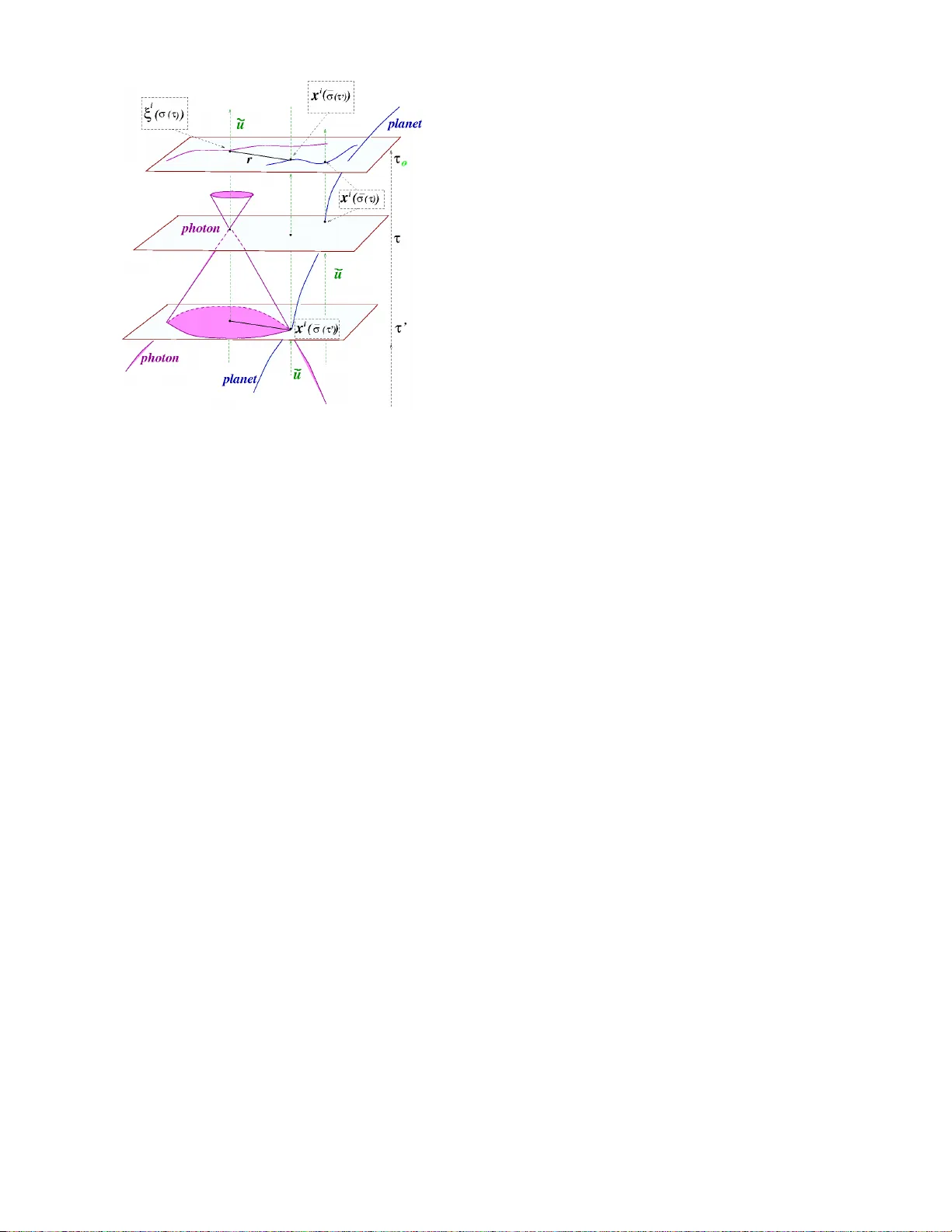
T racing ligh t propagation to the in trinsic accuracy of space-time geometry Mariateres a Crosta INAF, Astr onomic a l Obs ervatory of T orino via Osservatorio 20, I -10025 Pino T orinese (TO), Italy (Dated: July 25, 2018) Adv ancement in astronomical observ ations and tec hnical instrumentation requires coding ligh t propagation at high level of precision; this could open a new detection window of many subtle rela- tivistic effects suffered by li ght while it is propagating and entangle d in the physical measurements. Ligh t propagation and its subsequent detection should indeed be conceiv ed in a fully relativistic context, in ord er to interpret the results of the observ ations in accordance with the geometrical environmen t affecting light propagation itself, as an unicum surrounding universe. O ne of the most intrig uing asp ects is the b o ost tow ards the devel opment of highly a ccurate mo dels able to recon- struct the light path consistently with General Relativity and th e precepts of measurements. This pap er deals with the complexity of such a topic by sho wing ho w th e geometrical framew ork of mo dels lik e RAMOD , initially developed for astrometric observ ations, constitu t es an appropriate physical environmen t for b ac k tracing a ligh t ray conforming to the intrinsic accuracy of space-time. This article discusses the reasons why RAMOD stands out among the existent approaches applied to the ligh t p ropagation p roblem and pro vides a pro of of its capability in recasting recent literature cases. Keyw ords: r el ativity , gravita tion, space-time geometry , weak field appro ximations, l ight propag ation I. INTRO DUCT ION The treatment of light propag a tion in time-dep endent gravitational fields, as the surro unding universe, is ex- tremely impo rtant for astrophysics, encompassing is- sues from fundamental astronomy to co smology . Attain- ing very accur ate measurements will allow to observe a new range o f subtle physical effects (see, for example, Will [1], T uryshev [2], C r osta and Mignard [3], K op eikin and Gwinn [4], Kop eikin et al. [5, 6], Blanchet et al. [7], Kop eikin [8], Kopeikin and Mak arov [9], Damour and Nordtvedt [10], Damour et al. [11]). Undoubtedly , light tracing sho uld b e c o nceived in a general r e lativistic framework. T o day General Relativit y (GR) is the theory in which geometry and physics are joined together in order to explain how gravity w orks . The tr a jectory of a pho ton is trace d by solving the rela- tivistic equations of the null geo desic in a curved space- time and, at the same time, the detection pro ces s us u- ally takes place in a g eometrical en vironment gene r ated by a n-bo dy distribution as could b e that of o ur Solar System, i.e., by a lo caliz ed gravitationally-b ound distri- bution of mas ses moving with their velocities a nd a c cel- erations. Once the physical set-up is defined, the null geo desic s hould b e made ex plic it ac cording to the co rre- sp onding geo metry . Nevertheless the exact solution o f the null geo desic is not genera lly known. Hence, one has to resort to ap- proximation metho ds. Now adays several co nceptual ap- proaches mo de l the light propagation problem in the rel- ativistic context. Among them, the p ost-Newtonia n (pN) and the p ost-Minkowskian (pM) approximations are those mainly used (Ko pe ik in a nd Sc h¨ afer [12], Kop eikin and Mashho on [13], K lioner [1 4], T ey ssandier and Le Poncin-Lafitte [15]; and refer ences therein). The pec ulia r betw een the t wo approximations co ns ists in the fact that pN is based on the assumption of an everywhere-weak gravitational field and of slow motion, while the pM only on the weakness of the g ravitational field. This can b e fo rmalized [16] by saying that the expansion o f the metric tensor can b e characterized in powers of a sma ll pa rameter, 1/c in the pN case [17] a nd G in the pM approximation (whic h cont ains also terms in 1 /c). Basically the a pproximation methods rely up on the idea of b eing pN a s close a s p ossible to the New- tonian theory (abs o lute time, absolute space, a uxiliary Euclidean metric and instantaneous p otential) and pM to the Minko wskian interpretation o f spec ial r e lativity (absolute spa ce-time, auxilia r y Minko wskian metric and retarded p otential) [16]. In the framework of the pN approximation of GR, the light path is solved using a matching tec hnique which links the p erturb ed internal solution inside the near- zone of the n-bo dy system with the external one. Ap- plications of this metho d ar e adopted, for example, in [14, 18, 19], wher e the bounda ry conditions for the null geo desic ar e fix ed by the co o rdinate p osition o f the ob- server and imp osing the v alue of c to the mo dulus of the light ray vector at past n ull infinity . How ever, the expansion of the metric tensor may no t be ana lytic in higher pN appr oximations [16]. The seco nd pN approxi- mation in propag ation of ligh t w as inv estiga ted by Brum- ber g in [20]. Adv anc e ment on second order pN equa - tions of ligh t propaga tio n a re made in Xu et al. [2 1] or, more recentely , in T eyssandier [2 2]. Moreov er, the ana - lytical so lution for light propagation in the gr avitational field of one spher ic ally symmetric b o dy in the framework of p ost-p ost-Newto nian (ppN) developmen t ha s be e n re- analyzed [23]. Analytical for mulas hav e been compared with high-ac c uracy num eric a l integrations of the geo detic equations, the latter ba sed o n an approximation of the exact analytical solution. The author s found a deviation betw een the s tandard p ost-Newtonian a ppr oach a nd the high-accura cy numerical solution of the geo detic equa- 2 tions which amounts to 16 µ -arcs e c ond. As rep orted by Klioner and Zschock e [23], detailed analysis has sho wn that the error is o f pos t- p o s t-Newtonian order in co nt ra - diction with the ana lytical estimate. T o clarify the prob- lem, s ta ndard p ost-Newtonian and p ost-p os t-Newtonian solutions have been derived by retaining ter ms o f rele - v a nt analytica l orders of magnitude. F or ea ch individual term in the relev an t formulas exa c t analytical upper es- timates hav e b een found and a compact analytical so lu- tion for light propagatio n is derived up to 1 µ -a rcsecond accuracy . The e nhanced p ost-p ost-Newto nian terms cal- culated by Klioner and Zschocke, are confirmed r ecently by T ey s sandier [24 ] On the other hand, Kop eikin and Sch¨ afer [12], using the pM approximation, solve Einstein’s eq ua tions in the linear reg ime by expre s sing the p erturb ed par t o f the metric tensor in ter ms o f retarded Lienard- W eichert p o- ten tials. Later, Kop eikin a nd Mashho on [1 3] included all the relativistic effects related t o the gra vitoma gnetic field pro duced by the translatio na l velo city/spin-dependent metric terms. In these works a sp ecial tec hnique of in- tegration of the equation of light pro pagation [25 ] with retarded time argument is extended b oth outside and in- side of a gr avitating system o f ma ssive p oint-lik e particles moving a lo ng arbitrar y world lines. The null geo desic is rewritten as function of tw o independent parameter s, one rela ted to the Euclidean scalar pro duct betw een the light ray direction and its unperturb ed tra jectory , a nd the other derived a s the constant impact parameter [2 6] of the unper tur bed tr a jecto ry o f the light ray . Then, the light tr a jectory is again trac e d as a straight line plus in- tegrals, eac h co nt aining the perturbatio ns encountered, from a source at an ar bitr ary dis tance from an o bs erver lo cated within the n-b o dy system. As a conseque nc e , one more difference b etw een the pN/pM approximations app ears in the computation of the lig h t deflection contributions: in the pN scheme this is done by combining the exter nal and internal solution with the technique of asymptotic matching, while the pM metho d utilizes in addition a semi-ana lytical integration of the equation of light propagatio n from the obser ver to the source with resp ect to the retarded time considered as argument in the metric tensor. The rela tivistic p er - turbations r emain expressed in terms of in tegra ls (i.e. a semi-analytica l solution) whic h can b e solved analytica lly in sp ecific cases (i.e. not expr essed as a general s o lution of the differen tial equation, but as particular solutions for so me effects o n the light propag ation) once the mo- tion o f the gravitating bo dies is prescrib ed. The pM ap- proximation is also used b y T eyss andier and Le Poncin- Lafitte [27] that found a wa y to bypass the solution of the null geodesic in for m of differential equations. In this work the authors elab or a te the light tra jecto r y with the powerful tool of the Time T r ansfer F unction [28], work ed out thr oughout a recur s ive pro ce dur e for expanding the Synge’s W or ld F unction, a cov ar iant metho d that is con- ceptually muc h clos er to that of RAMOD, the appr oach discussed in the present work. RAMOD stands originally for Relativistic Astrometric MODel, c o nceived to so lve the inv ers e r ay-tracing prob- lem in a general relativistic fra mework not constra ined by a priori approximations. RAMOD is, actually , a fam- ily of models of increas ing int rinsic accuracy all based on the geometr y of curved ma nifo lds ([29, 30] and reference there-in) wher e , as this pap er proves, light pr opagatio n can b e ex pressed in a gener al relativistic co n text. An analytical solution o f the n ull geo desic exists in the cas e of the Parametrized-Post-Newtonian Sch warzsc hild met- ric [1, 31], which, just c o nsidering the s pher ical mass of the Sun, can b e implemen ted for the Gaia missio n (Esa, T ur on et al. [32]) and co uld prov e the dilaton-runawa y scenario [33]. A t present, the RAMO D full solution re- quires the n umerica l in tegr a tion of a set of coupled non linear differential equations , called “ma ster equations” , for tracing back the light tra jectory to the initial position of the sta r , a nd which naturally entangles the contribu- tions of the cur v a ture o f the bac kgr ound geo metr y . A solution o f this system o f differential equa tions contains all the relativistic perturba tio ns suffered by the photon along its tra jectory due to the intervening gravitational fields. The bo undary condition are usually fixed by the required ph ysical mea surement [34]. In this context, a semi-analytica l solution w as found by de F elice and P reti [35]. This work shows how RAMOD can natura lly recover the seminal w ork of Kop e ikin and Sc h¨ afer [12] a nd Klioner [14] . While the thir d one stems from the g e n- eral fo rmulation of the second by co nforming to its ba- sic conception [18], RAMOD resp onds to an inherently different strategy . As far as the invers ligh t ray trac- ing pr o blem is concerned, in the Kop eikin a nd Sh¨ afer and Klioner approa ch es the ligh t ray is recons tructed as a sum of terms whic h allows for a direct ev alua tion o f the individual relativis tic effects, induced by the gr av- itating b o dies, suffere d by the light on its wa y to the observer. RAMOD, instea d, a ims to determine a full s o- lution fo r the light tra jector y which naturally include, in a curved space-time, all the individual effects; the latters are somewhat hidden in the cov ariant forma lism o f this approach a nd direc tly co n tribute to the solutions of the master equations . Evidently , an y s pec ific effect one is in- terested to explore can b e independently deduced from our forma lism as a branch output, once we adapt the mo del to a required spec ific case. A pro of of this is given in Cr o sta and V ecchiato [36], wher e a fir st co mparison betw een RAMOD and GREM (Gaia RElativistic Mo del, [14], which employ es the pN formulation) w as carried out via the extrap olatio n of the aber rational ter m in the ”lo - cal” light direction, i.e., at the obser ver. Now, if w e consider a gravitational field genera ted by a n-b o dy system, the req uired accur acy in back trac- ing the light ray should be consistent with the geo me- try induced by the system itself. The accuracy is gaug ed by the virial theorem, i.e., by the ratio v / c , where v is the t ypical velocity of a bo dy o f the s ystem. In this re- sp ect, RAMOD3 [29] is dev elop ed up to the order ( v/c ) 2 , 3 namely , it is based on a static geometry of the spa ce-time, whereas the most recent RAMOD4 [30] is the extension of the predecessor to include a dynamical geometry (i.e., all metric terms up to the or der ( v /c ) 3 ), which is ac- complished b y including also the vorticit y con tribution prop ortiona l to the off-diag onal ter m g 0 i of the metric. Both mo dels introduce the retar ded co nt ributions to the metric due to the gravitational influence of the sources on the light path, a ccording to the natural space- time structure. In s ection I II , we discuss how to build an appropria te geometrical set-up in order to handle light propaga tion through such a space-time. In section IV we present the building pro cess o f the differen tial eq uations, i.e., the ma ster equatio ns, from which the lig h t tra jec- tory from an o bserver, lo c a ted within the n-b o dy sys tem, to a dis tant sta r can b e r econstructed. W e distinguish t wo cases: (i) the static s pace-time (RAMOD3), and (ii) its dynamical ex tension (RAMOD4). An applicatio n o f RAMOD3 to the euc lide a n metr ic is presented in sec tio n V, while sectio n VI shows ho w this las t co mputation a l- lows to para metr ize the RAMOD3 master equa tion as done in [1 2]. Finally , section VI I shows how the v elo c- it y of the b o dies can enter the metric term simply as a ”retarted distance” corrections in RAMOD3-like mo dels . II. NOT A T IONS In this pap er the following notations will b e used: • components of v ector ial q uantit ies are indicated with indexes (no b o ld symbols ), where the la tin in- dex stands for 1,2,3 and the gree k ones for 0,1,2 ,3; • regular bo ld indica tes fo ur-vector (e.g . u ); • indexes are r aised and lo wered with the metric g αβ ; • n i n i or n i n i stands for the scalar pro duct with re- sp ect to t he euclidean metric δ ij , whereas l α l α with resp ect the metric g αβ ; • c indicates the fundamental sp eed (equa l to the sp eed of light in v acuum); • A quantit y lik e ˙ Υ α , repres en ts the tangent vector to a curve Υ; • P ( u ) αβ represents the op erator which pro jects o r- thogonally to its argument. • x ′ α or x α indicate generic four-co ordinates, whereas ξ α the Lie- transp orted ones; • dot applied over coor dinates means de r iv ativ e with resp ect to the co ordinate time; • partial deriv ative with resp ect to the co o rdinates are usually indicated by a co mma. Instea d, the symbol ∂ is adopted in c ases where the for mulas need to b e more explicit a nd av oid confusion; co- v a riant der iv a tive a re indicated with ∇ . II I. SETTING UP THE GEOMETR Y The RAMOD framework is ba sed on the small cur- v a ture limit, for which the cur v a ture of the ba ckground geometry is sufficient ly small to neglect non linear terms. The degree o f this approximation has in turn to b e s pe- cialized to the particula r cas e one wishes to mo del. The first step is to identify the gravitational sources and then fix the background geometry . Let the space-time b e gener ated b y a weakly r elativis- tic g ravitationally b o und sy stem; in this case the metric is g αβ = η αβ + h αβ + O ( h 2 ) , (1) where η αβ is the flat Minkowskian metric and the h αβ ′ s describ e effects g enerated by the b o dies of the sy stem and are smal l in the sense that | h αβ | ≪ 1. F ro m the viria l theorem all forms of energy density within the system m ust not exceed the maximum amo un t of the gr avita- tional p otential in it, say , U . So, the energ y bala nce requires that | h αβ | ≤ U /c 2 ∼ v 2 /c 2 , where v is the a v- erage re lative velo cit y within the sys tem [37]. Since the latter is weakly relativis tic [38], the h αβ ′ s are at le a st of the order of ( v /c ) 2 and the level of accuracy , to which is exp ected to extend the calculatio ns, is fixed b y the or der of the sma ll q ua nt ity ǫ ∼ ( v /c ). In summary , the p er tur - bation tensor h αβ contributes with terms even in ǫ to g 00 and g ij (low est order ǫ 2 ) and with terms o dd in ǫ to g 0 i (low est o rder ǫ 3 , Misner et al. 31); its spatial v ariations is on the order of | h αβ | , while its time v ariatio n is o n the o rder o f ǫ | h αβ | . Clearly the metric for m (1) is pre- served under to infinitesimal co o rdinate transfor mations of orde r | h | . Under these h yp othesis, in orde r to describ e the space- time evolution of the system, let us in tro duce a family of ph ysica l o bservers, i.e. a time-lik e c o ngruence of curves, and consider its vorticit y , which measur es ho w a world- line o f an observer rotates around a neighboring one. If an op en set of the space- time manifold admits a vorticity- free co ngruence of lines, then it can b e foliate d (F ro benius theorem, [3 9, 40]). Given a general co o rdinate s pa ce-time representation ( x ′ i , t ′ ) i =1 , 2 , 3 , the asso ciated metric b eing g ′ αβ ( x ′ , t ′ ), there exists a family of three-dimensional hypersur faces S ( τ ), o r slic e , describ ed b y the e q uation: τ ( x ′ , t ′ ) = constant , (2) where τ ( x ′ , t ′ ) is a rea l, smo oth and differentiable func- tion of the co ordinates . A spa ce-like foliation implies that a unitary one-form u ′ α exists whic h is everywhere pro po r- tional to the gradient of τ (figure 1), na mely [3 1, 39]: u ′ α = − ( τ ,α ′ )e ψ ′ (3) where g ′ αβ u ′ α u ′ β = − 1 , (4) 4 and e ψ ′ = [ − g ′ αβ ( τ ,α ′ )( τ ,β ′ )] − 1 / 2 . (5) τ (x’, t’) = constant S ( ) τ (x’, t’) FIG. 1. A co ordinate grid ( x ′ , t ′ ) and the hyp ersurface τ ( x ′ , t ′ ) = constant. Evidently the curves tangen t to the v ector field, i.e. u ′ α = g ′ αβ u ′ β , form a congruence of time-like lines C u ′ , everywhere orthogo nal to the slices S ( τ ). Le t us compute the vorticity a s the tensor quantit y [39] ω αβ ≡ P ′ α ρ P ′ β σ u ′ [ ρ,σ ] , (6) where sq uare brackets mean anti-symmetrization and P ′ αβ ( u ′ ) = g ′ αβ + u ′ α u ′ β (7) is a pr o jector op erato r on S ( τ ). Since u ′ [ α,β ] results in u ′ [ α ∂ β ] ψ ′ , we find that the congr ue nc e C u ′ is v or ticit y- free only up to ( v /c ) 2 order; namely , ω αβ = P ′ α ρ P ′ β σ u ′ [ ρ ∂ ′ σ ] ψ ′ = O ( h 0 i ) . (8) Then, we may affirm that consider ing o nly terms up to ǫ 2 ∼ ( v /c ) 2 , it is the same a s assuming that s tructure of space-time is sta tic. So, do es the one-form u ′ α hav e a ph ysical meaning? Let us introduce a new co ordinate system ( x 0 , x i ) such that: ( x 0 = τ ( ~ x ′ , t ′ ) x i = x i ( ~ x ′ , t ′ ) (9) where x i are the spa ce-like co o rdinates defined on ea ch slice. F rom (9), the co ngruence of normals now have the following tangent v ector field:    u α ( x 0 , x i ) = − δ 0 α e ψ u α ( x 0 , x i ) = − g 0 α e ψ = dx α dσ (10) where ψ = ψ ( x 0 , ~ x ) is a unitary function ( u α u α = − 1), σ is the parameter o n the nor mals, and u α ( x 0 , x i ) = ∂ x ′ β ∂ x α u ′ β ( x ′ , t ′ ) = − ∂ τ ∂ x α e ψ ′ ( x ′ ,t ′ ) = − δ 0 α e ψ ( x 0 ,x i ) . (11) Clearly it is e ψ = dσ dτ =  − g 00  − 1 / 2 (12) which means that the para meter σ runs unifor mly with the co ordina te time τ . The congr uence C u , how ever, do es not Lie-tr ansp ort the spatial c o ordinates x i . F rom (9) and (A2), the line element can b e cast into the form: ds 2 = − ( N dx 0 ) 2 + g ij ( dx i − N i dx 0 )( dx j − N j dx 0 ) (13 ) where N ≡ ± 1 / u 0 and N i = u i /u 0 are termed resp ec- tively lapse a nd shift functions (or factor s) [31]. In fact, choosing at time τ 1 , say , a n arbitrary even t P , la bele d by the co o rdinates ( τ 1 , x i 1 ), the unique normal throug h that po in t will intersect the slice S ( τ 1 + ∆ τ ) at a p oint P ′ with spatial co o rdinates which ar e s hifted fr om the initial o nes by the a mount (s e e app endix A): ∆ x i = Z ∆ τ 0 N i ( τ ′ ) dτ ′ . (14) The spatia l coordinate tr ansformation to be applied, in order to make the shift factor v anish and assure that the congruence of no r mals will now Lie-tra nsp ort the spatia l co ordinates, is: ( dξ i = dx i − N i dx 0 dξ 0 = dx 0 = dτ , (15) in which we impos e: ˜ u α ( ξ 0 , ξ i ) = ∂ ξ α ∂ x β u β ≡ e φ δ α 0 . (16) Under the ab ov e transforma tio n, we clearly ha ve for α = 0:  ∂ ξ 0 ∂ τ g 00 + ∂ ξ 0 ∂ x i g 0 i  e ψ = − e φ = ⇒ e φ = p − g 00 from (12); and for α = i ∂ ξ i ∂ τ u 0 + ∂ ξ i ∂ x j u j = ∂ ξ i ∂ τ g 00 + ∂ ξ i ∂ x j g 0 j = 0 . But it is: ˜ g 0 α = ∂ ξ 0 ∂ x ρ ∂ ξ α ∂ x σ g ρσ = ∂ ξ α ∂ x σ g 0 σ 5 which implies ˜ g 00 = g 00 (17) ˜ g 0 i = ˜ g 0 i = ∂ ξ i ∂ τ g 00 + ∂ ξ i ∂ x j g 0 j = 0 . (18) Then the vector field tangent to the congruence C ˜ u which transp orts the spatial co ordina te is:      ˜ u α ( ξ 0 , ξ i ) = dξ α dσ = e φ ( τ , ~ ξ ) δ α 0 ˜ u α ( ξ 0 , ξ i ) = e φ g 0 α = − e ψ ∂ τ ∂ ξ α . (19) Let us summarize. First, the v or ticit y is prop ortiona l to the g 0 i term of the metric, the low est order e s tablished by equation 8 ; sec o nd, we must b ear in mind that, even if metric for m (1) holds up to infinitesimal co ordinate transformatio ns, the c ondition that the shift factor is zer o is pr eserve d u nder the ab ove tra nsformation only to the or der ǫ 2 . In fact, to the order of ǫ 3 , the terms g ′ 0 i will not remain zero if they were so initially . W e may a ffirm that considering only terms up to ǫ 2 ∼ ( v /c ) 2 , it is the s ame as assuming that structure o f spa ce-time is static, since a static space-time is a sta tionary s pacetime in which the timelike Killing vector field has v anishing vorticit y , or equiv alen tly (by the F r ob enius theore m) is hyper surface orthogo nal, i.e. admits a family of spacelike surfac es o f constant time ([29, 3 1, 39]). The pa r ameter σ alo ng the Killing congruence C ˜ u , such that ˜ u α = dξ α /dσ , is the prop er time of the physical obser vers who Lie-transp ort the spatial co o rdinates. Any h yp ersur fa ces, at each dif- ferent co ordinate time τ , can be considered the rest space of the observer ˜ u . O ne ca n require that the w or ld line of the cen ter of mass o f the b o dy’s system, chosen a s o ri- gin of coo rdinates of the gravitational b ounded system, belo ngs to this congruence while the world lines of the bo die s would differ fro m the curves of the congruence by an amount which depends on the lo cal s patial velo c ity relative to the center of mass; how ever, at the ǫ 2 order, i.e. neg lecting the relative motion of the gravit y so ur ces, one can assume that also their world lines b elo ng to that congruence a nd the geo metry that eac h photon feels is, then, identified with the metric ˜ g αβ . T o the order of ǫ 3 the shift factor should be retained and so also terms pro- po rtional to h 0 i (eq. 8). Since we requir e that the back- ground geometry is weakly relativistic, we can assume that the vorticit y is free up to the ǫ 3 order only lo cally; then the space-time still admits a family of h yp ersurfac e s τ =c onstant with normals f or ming a congr uence of curv es with tangent field u given b y (10). The g iven co ordinate system ( x i , τ ), where x i are fixed o n each slice, is still centered to the baricenter o f the n-b o dy system, but, o n the other hand, each slice is not the lo cal rest-space of the obser ver u . These normals do no t in gener al Lie- transp ort the spatia l co ordinates x i ; instead they v ary along the normals acco rding to the shift law (14). Any of these observers ca n b e conside r ed at rest with resp ect to the co or dina tes x i only lo c al ly , and for this reason u is called lo c al b aryc ent ric observer . IV. FROM THE NULL GEODESIC TO THE MASTER EQUA TIONS In the following sections we drop the tilde for the met- ric. A photon trav elling fro m a distant star to an ob- server, lo cated w ithin the bo unded sy stem, would s ee the space-time a s a time developmen t of the τ = co n- stant slices. Let us now co nsider a null geo desic Υ k with tangent vector field k α ≡ dξ α /dλ which satisfies the fol- lowing eq uations: k α k α = 0 (20) dk α dλ + Γ α ρσ k ρ k σ = 0; (21) here λ is a real parameter on Υ k and Γ α ρσ are the con- nection coefficie nts o f the given metr ic. Assume that the tra jectory starts at a po int P ∗ on a slice S ( τ ∗ ) (say) and with spatial co or dinates ξ i ∗ . The null geo desic cr o sses each slice S ( τ ) a t a p oint with co or dinates ξ i = ξ i ( λ ( τ )); but this p oint also b elongs to the unique nor mal to the slice S ( τ ), cro ssing it with a v alue o f the parameter σ = σ ( ξ i ( λ ) , τ ) ≡ σ ξ i ( λ ) ( τ ) (figur e 2). Let us now de- FIG. 2. The p oint ξ i ( λ ( τ )) b elongs to the null geo desic but also to the un ique normal to the slice S ( τ ) crossing it with a v alue of th e parameter σ ξ i ( λ ) ( τ ). fine the one- parameter lo cal diffeomorphism [3 9]: φ ∆ σ ≡ φ ( σ ξ i ( λ ) ( τ 0 ) − σ ξ i ( λ ) ( τ )) : Υ k ∩ S ( τ ) → S ( τ 0 ) (22) which ma ps each p oint on the null geo desic Υ k with the po int on the slice S ( τ o ) which one gets to by moving along the unique no r mal through the p oint Υ k ( λ ) ∩ S ( τ ), by a parameter distance ∆ σ = σ ξ i ( λ ) ( τ o ) − σ ξ i ( λ ) ( τ ) (figure 3). Since t he spatial coordinates ξ i are Lie-transp orted alo ng the no r mals to the slice s , then the points in S ( τ 0 ), which are ima ges of those on the null geo desic under φ ∆ σ , have co ordinates ( φ ∆ σ (Υ k (( λ ) ∩ S ( τ ))) i = ξ i . The curve in S ( τ 0 ) which is the image o f Υ k under φ ∆ σ , is : ¯ Υ ≡ φ ( σ ξ i ( λ ) ( τ o ) − σ ξ i ( λ ) ( τ ) ) ◦ Υ k , (23) 6 with tang ent vector [3 9] ˙ ¯ Υ α = ˙  φ ∗ ∆ σ ◦ k  α = ∂ ξ α ( σ ( τ o )) ∂ ξ β ( σ ( τ )) k β ≡ ℓ α . (24) This coincides with the pro jection op era tio n on the rest-space o f the observer ˜ u in any p oint o f the mapp ed tra jectory on the s ilde: ℓ α = P ( ˜ u ) α β k β , (25) hence the c urve ¯ Υ is the spatial pro jection of the null geo desic on the slice S ( τ o ) at the time o f observ ation; this curve will b e denoted as ¯ Υ ℓ and is naturally par am- eterized by λ . Then from equation (24) b y using (1 9) (where ˜ u α ˜ u α = − 1) o r (25), it follows that: ℓ α = k α + ˜ u α ( ˜ u β k β ) . (26) Clearly b y setting α = 0 and from equation (19) we de- duce ℓ 0 = 0; mor eov er, ℓ α is space- like as exp ected as it is a pro jection on slice S ( τ 0 ) and lies everywhere in it. Since each point of ¯ Υ ℓ is the ima g e under the diffeomor - phism φ ∆ σ of a po int Υ k ∩ S ( τ ), it is mor e conv enient to label the p o int s of ¯ Υ ℓ with the v alue of the parameter σ ξ i ( λ ) ( τ ) which, a s we have alr eady said, uniquely iden- tifies that point on the normal to the slice S ( τ ) which contains it. Hence, b eing dσ = − ( ˜ u α k α ) dλ , (27) we de fine the new tangent vector field: ¯ ℓ α ≡ dξ α dσ ξ i ( λ ) = − ℓ α  ˜ u β k β  . (28) In the sa me wa y we denote ¯ k α ≡ − k α ( ˜ u β k β ) (29) so that ¯ k α = ¯ ℓ α + ˜ u α (30) which implies: ¯ ℓ α ¯ ℓ α = 1 . (31) Note that the parameter σ ξ i ( λ ) is also the one which makes the tangent to the curve ¯ Υ unitary . T o shor t the notations, in what follows we deno te σ ξ i ( λ ) as σ . W e can now write the differen tial eq uation which is satisfied b y the v ector field ¯ ℓ . F ro m (27) and (29), equations (21) bec omes (see app endix B): d ¯ ℓ α dσ + d ˜ u α dσ − ( ¯ ℓ α + ˜ u α )( ¯ ℓ β ˜ u τ ∇ τ ˜ u β + ¯ ℓ β ¯ ℓ τ ∇ τ ˜ u β ) + Γ α β γ ( ¯ ℓ β + ˜ u β )( ¯ ℓ γ + ˜ u γ ) = 0 . (32) FIG. 3. The curv e ¯ Υ is the image of the null geo d esic Υ k under the diffeomorfism φ ∆ σ . In this equa tion the quan tity ¯ ℓ β ¯ ℓ τ ∇ τ ˜ u β can be written explicitly in terms of the ex pansion Θ ρσ of C ˜ u [29], a s: d ¯ ℓ α dσ + d ˜ u α dσ − ( ¯ ℓ α + ˜ u α )( ¯ ℓ β ˙ ˜ u β + Θ ρσ ¯ ℓ ρ ¯ ℓ σ ) + Γ α β γ ( ¯ ℓ β + ˜ u β )( ¯ ℓ γ + ˜ u γ ) = 0 (33) where Θ ρσ = P α ρ P β σ ∇ ( α ˜ u β ) [39]. Since the only non v an- ishing comp onents of the expa nsion a re Θ ij = (1 / 2) ∂ 0 h ij , the expansion v anishes identically as conse q uence of the assumption to neglect time v ariatio ns o f the metric . F r om this condition equation, after some algebra , (33) bec omes to the required order (see a ppendix C): d ¯ ℓ α dσ + d ˜ u α dσ − ( ¯ ℓ α + ˜ u α )( ¯ ℓ β ˙ ˜ u β ) + Γ α β γ ( ¯ ℓ β + ˜ u β )( ¯ ℓ γ + ˜ u γ ) = 0 . (34) If α = 0, equation (32) leads to d ¯ ℓ 0 dσ = 0 as suring tha t condition ¯ ℓ 0 = 0 ho lds true all along the curve ¯ Υ; if α = k equation (32) gives the set of differen tial equations that we need to integrate to identify the star or the ph ysical e f- fects related to ligh t propag ation (see deta ils in appendix D, [41] and [29]): d ¯ ℓ k dσ = − ¯ ℓ k  1 2 ¯ ℓ i h 00 ,i  − δ ks  h sj,i − 1 2 h ij,s  ¯ ℓ i ¯ ℓ j + 1 2 δ ks h 00 ,s . (35) These equatio ns de ter mine lig h t pr o pagation in the static cas e, her e and after called RAMOD3 master equa- tions. Let us remar k , that this definition do es not stand for the “ master equation“ used in classica l or quantum ph ysics ; in this context it represents a set of firs t-order nonlinear diff erential equation describing ev olution of the spatial lig h t direction compo nent s accor ding to the pre- scrib ed geometry . In the dynamical cas e, a ny “lo cal“ 7 observers u which are at rest with r esp ect to the co or - dinates x i lo cally , once intersected by the null ray will se e the light sig nal alo ng a spatia l direction ℓ in his re st space given by (more details can b e fo und in de F elice et al. [30]) ℓ α = P α β ( u ) k β ( τ ) (36) where P ( u ) α β = δ α β + u α u β this time is the op er ator which pro jects orthogo nally to the u ’s. F ollowing the same reasoning of the static case, we para meterize the curve Υ with the parameter σ whic h makes unitary the lo cally pr o jected vector field ℓ whic h w e term again ¯ ℓ , so ¯ ℓ α ¯ ℓ α = 1. The differen tial e quation of the null ray , written in ter ms of ¯ ℓ α , is still given by (32), the only difference being that h 0 i 6 = 0, h 00 , 0 6 = 0, and h ij, 0 6 = 0. After so me algebr a, equation (32) now reads : d ¯ ℓ 0 dσ − ¯ ℓ i ¯ ℓ j h 0 j,i − 1 2 h 00 , 0 = 0 (37) d ¯ ℓ k dσ − 1 2 ¯ ℓ k ¯ ℓ i ¯ ℓ j h ij, 0 + ¯ ℓ i ¯ ℓ j  h kj,i − 1 2 h ij,k  (38) + 1 2 ¯ ℓ k ¯ ℓ i h 00 ,i + ¯ ℓ i ( h k 0 ,i + h ki, 0 − h 0 i,k ) − 1 2 h 00 ,k − ¯ ℓ k ¯ ℓ i h 0 i, 0 + h k 0 , 0 = 0 . These equations are named RAMOD4 master equations. Note that in RAMOD4, with respect to RAMOD3, we hav e one more differe ntial equatio n fo r the ¯ ℓ 0 comp onent. T e r m like h k 0 , 0 is redundan t at the order of ǫ 3 , but w e keep it in order to c o mpare the ge o desic equations, as it will b e clear in section 6. V. P A RAMETRIZED MAPPED TRAJECTORIES Let us fix the o r igin of the co or dinates and consider it as the center o f mass (CM) of the matter distribution of the n-b o dy system. Let us, also, choice that its spatia l co ordinates b elong to the congr ue nc e o f cur ves C ˜ u . FIG. 4. Mapp ed ph oton tra jectory in a slice τ 0 and normal neighbourho od of the origin of th e spatial co ordinates ξ i (CM) Assume t hat the mapped spatial photon tra jectory ¯ Υ ¯ ℓ , in the slice τ = τ 0 , b elong s to a normal neighbourho o d of CM. By definitio n then, there exist a unique geo desic (in any case space like geo desic) Υ ′ connecting CM to any point P o f ¯ Υ ¯ ℓ . Denoting with σ ( τ , ξ i ) the par ameter along ¯ Υ ¯ ℓ , with Λ the par ameter along each of the curves Υ ′ stemming f ro m CM and such that Λ C M = 0, and with ϕ the homeomorphism which defines the chart co n taining P in the nor mal neighbourho o d of CM, we hav e [39]: P = ¯ Υ( σ ) = Υ ′ (Λ) = ϕ − 1 ( ξ i ( σ )) . The co or dinate ξ i can b e ex pressed as: ξ i = ϕ i ( P ) = [ ϕ ◦ ¯ Υ( σ )] i = [ ϕ ◦ Υ ′ (Λ)] i . Applying to b oth members of the ab ove equation the map Υ ′ − 1 ◦ ϕ − 1 , we obtain : Λ = (Υ ′ − 1 ◦ ϕ − 1 ) ◦ ( ϕ ◦ ¯ Υ( σ )) = Λ( ξ i ( σ )) , namely the Λ implicit dep endence on σ at the p oint P with co ordina tes ξ i . Denoting as ζ i ≡ dξ i d Λ , the unit ta n- gent to the c ur ve Υ ′ , we define the length of Υ ′ betw een CM a nd P as the qua nt ity: L = Z Λ( ξ i ( σ ) 0 ( ζ i ζ i ) 1 / 2 d Λ ′ ≡ Λ( σ ) . (39) The po int o f closest approa ch of the photon to the cen ter of mass, will cor r esp ond to the minimum of L . Thus, differentiating (39) with resp ect to σ , we hav e  dL dσ  P = ( ζ i ) P ¯ ℓ i , and at the p oint of clos est appro ach with para meter ˆ σ ( ζ i ¯ ℓ i ) ˆ σ = 0 . (40) Let us s e t Λ( ˆ σ ) ≡ ˆ ξ as the impact par ameter which r ep- resents the dista nc e fr om P ( ˆ σ ) to CM; this is a constant which lab els ea ch mapp ed photon tra jectory on an y given slice τ = τ 0 . Recalling that ξ i (Λ( σ )) = ξ i ( σ ) at any p oint P of int ers ection of the curv es ¯ Υ with the curv e Υ ′ , then, at CM, wher e ξ i C M = 0 and Λ C M = 0, w e ha ve to the first or der in Λ: ξ i (Λ + δ Λ ) = ξ i (Λ C M ) +  dξ i d Λ  Λ C M δ Λ + ... =  ζ i 0  ( C M →P ) δ Λ + ... (41) where  ζ i 0  ( C M →P ) refers to the ta ngent v ector at the origin of the “unique” spacelike ge o desic connecting CM, the o rigin, to the p o int P . F r om (41) we clearly have: ξ i (Λ) =  ζ i 0  ( C M →P ) Z Λ 0 d Λ =  ζ i 0  ( C M →P ) Λ (42) 8 Let us aga in introduce a new par ameter on ¯ Υ, namely ˆ τ ≡ σ − ˆ σ then, a t a p oint P on ¯ Υ with pa rameter ˆ σ + δ ˆ τ ξ i ( ˆ σ + δ ˆ τ ) = ξ i ( ˆ σ ) +  dξ i d ˆ τ  ˆ τ =0 δ ˆ τ + ... (43) But fro m (42), at Λ( ˆ σ ), it is also ξ i (Λ( ˆ σ )) =  ζ i 0  ( C M → P ) ˆ ξ ≡ ˆ ξ i (44) hence, at any p oint P on Υ, we obtain ξ i ( σ ) = ˆ ξ i + Z ˆ τ 0 ¯ ℓ i d ˆ τ ′ , (45) i.e., the co ordinate path of the pho ton o n the slice τ 0 as function of the t wo parameter ˆ ξ i and ˆ τ . F ormula (45) has bee n o btained for a mappe d tr a jectory and it contains the lo cal spa tial directio n in integral form. I n this se ns e gen- eralizes the parameter ization of Ko p e ikin and Mashho o n [13] (and a n y references ther ein), wher e, instead, the Eu- clidean scalar product is used (i.e. ¯ ℓ i ¯ ℓ i = δ ij ¯ ℓ i ¯ ℓ j ). Hence, if the euclidean scala r pro duct is a pplied and in case of constant light direction, equation (4 5) is identically the same. How ever, by calculating the square mo dulus of (45) we get r 2 = ξ i ξ i = ˆ ξ 2 + ˆ τ 2 . (46) The rea de r should b ear in mind that equation (45) has its v alidit y only up to ǫ 2 and can b e traced onto the hypersurface wher e the photon’s tra jectory is mapp ed. VI. NULL GEODESICS IN COMP ARISON The quantit y ¯ ℓ α (eq. 28) in RAMOD is the unitary four-vector repr esenting the lo c al line-of-sight of the p ho- ton as measured by the loca l observer u , at rest with re- sp ect to the bar ycenter o f the n-b o dy system. In shor t, it re pr esents a physical entit y . Scop e of this section is to demo nstrate, fir s t, that substituting its co o rdinate counterpart, within the appropria te a pproximations, to equation (38) o f RAMOD4 is equiv alent to recover light geo desic equation in the first p ost-Minko wskian regime adopted in K o pe ikin and Mas hho o n [1 3] or Ko peik in and Sch¨ a fer [ 12]. Seco nd, the above authors parametrize the co or dinate expression of the nu ll geo desic to solve the light pr opagation problem in many physical context, as the literatur e la rgely shows, but, as far as RAMOD is concerned, only equation (35) of RAMOD3 recov ers the parametrized one (37) in Kop eikin and Mashho on [13] (equiv alent to equation (19) in Ko peik in and Sc h¨ afer [12]). Nevertheless, let us use the definition of ¯ ℓ α ; s inc e it is ¯ ℓ i = − k i u α k α ≈ − k i u 0 k 0 [ − 1 + h 00 + h 0 i ( k i /k 0 )] , with u 0 = ( − g 00 ) − 1 / 2 and k i /k 0 = d x i / d x 0 , the spatial co ordinate comp onents of ¯ ℓ i result (in wha t follo ws we assume c = 1): ¯ ℓ i = ˙ x i ( − g 00 ) 1 / 2  1 − h 00 − h 0 i ˙ x i  − 1 = ˙ x i  1 + 1 2 h 00 + h 0 i ˙ x i  + O  h 2  . (47) Let us transform e q uation (38) of RAMOD4 into its coor - dinate expres sion and co nsider o nly its s pa tial par t. Ne- glecting all the co nt ributions no n linear in h , from (47) and (12) the left-hand s ide r esults: d ¯ ℓ k dσ ≈ d dτ  ˙ x k (1 + 1 2 h 00 + h 0 i ˙ x i )  = ¨ x k (1 + 1 2 h 00 + h 0 i ˙ x i ) + ˙ x k  1 2 dh 00 dτ + dh 0 i dτ ˙ x i + h 0 i ¨ x i  = ¨ x k + ˙ x k  1 2 h 00 ,i ˙ x i + 1 2 h 00 , 0 + h 0 i,j ˙ x i ˙ x j + h 0 i, 0 ˙ x i  + O ( h 2 ) , (48) while the rig ht -ha nd- side tr ansforms as: 1 2 ˙ x k ˙ x i ˙ x j h ij, 0 − ˙ x i ˙ x j  h kj,i − 1 2 h ij,k  − 1 2 ˙ x k ˙ x i h 00 ,i − ˙ x i ( h k 0 ,i + h ki, 0 − h 0 i,k ) + 1 2 h 00 ,k + ˙ x k ˙ x i h 0 i, 0 − h k 0 , 0 (49) Equating expres sions (48) and (49) we get the appr ox- imated null geo desic equatio n (40) in Kop eikin and Sch¨ a fer [1 2] (and references therein), namely in co or di- nate form: ¨ x k ≈ 1 2 h 00 ,k − h 0 k, 0 − 1 2 h 00 , 0 ˙ x k − h ki, 0 ˙ x i − ( h 0 k,i − h 0 i,k ) ˙ x i − h 00 ,i ˙ x k ˙ x i −  h ki,j − 1 2 h ij,k  ˙ x i ˙ x j +  1 2 h ij, 0 − h 0 i,j  ˙ x i ˙ x j ˙ x k . (50) W e remind that the term ¨ x k is of the order of h b eca use of the order of the geo desic equation itself. A ctually , this la st r esult should b e exp ected, since both equations, (38) of RAMOD4 and (40 ) in Ko pe ikin and Sch¨ afer [12], are deduced from the nu ll geo des ic (2 1 ) in a weakly field regime. Once obtained this equiv alence at the h o r der by using the co or dinate expression (47) of ¯ ℓ , in principle one could a dopt the sa me para meter ization done, for in- stance, b y Kop eikin and Mashho on [13] (equation (36), or [9], equatio n (7 ) and referenc e therein) in order to find a solution of the master equatio n in the RAMOD framework a pplicable to all of the physical cases already 9 presented in the literature in this context. These para me- ters are: (i) τ , defined as the Euc lide a n scalar pro duct b e- t ween the light ray vector and its unp erturb ed tra jectory (eq. (13) in [13], for example), treated as a no n- affine pa- rameter, and (ii) ˆ ξ = ˆ ξ i ˆ ξ i , the constant impac t pa r ameter of the unp er tur bed tra jectory of the light ray . But as sec- tion V shows, this k ind of parameter ization in RAMOD is p o ssible only in a static space- time wher e null geo desic can b e ent irely mapped in to a hypersurface simultaneous to the time of obs erv ation, i.e. at the ǫ 2 level of ac curacy in the linear regime. Then, c o nsistently to the previous reasoning , we need to chec k if RAMOD3 master eq ua- tion can be transformed in to eq. (36) of Ko p eikin and Mashho on [13]. Ther e fo re, let us adopt the parameter i- zation (45) in case of a co nstant light direction, say ℓ i 0 ; moreov er, let us intro duce the impact para meter ˆ ξ k as done in [25], i.e. a s sume the equiv a lence of the tw o pa- rameteriza tio ns as a conseq uence of the following change of c o ordinates: ˆ ξ k = P k i ξ i − ℓ k 0 ˆ τ + Ξ k , ˆ ξ 0 = ˆ τ . (51) In this transfor mation the impact pa rameter ˆ ξ k is as- so ciated to the coo rdinate pro jected ortho gonally (with resp ect to the light direction) by the op era tor P α β = δ α β − ℓ α ℓ β ; Ξ k represents a cor rection to the co ordinates of the same or der o f the p erturbation term | h | o f the metric, and d ˆ τ = dσ . Once a dopted such a new co ordinate sys - tem, the partial deriv a tives should also change a ccording to the following rule: ∂ ∂ ξ i = ∂ ˆ ξ j ∂ ξ i ∂ ∂ ˆ ξ j + ∂ ˆ ξ 0 ∂ ξ i ∂ ∂ ˆ ξ 0 = P j i ∂ ∂ ˆ ξ j + Ξ i ,j . (52) The nex t step is to compute the new co mpo ne nts o f the metric h αβ according to transfo r mations (51): h 00 = ∂ ˆ ξ 0 ∂ ξ 0 ∂ ˆ ξ 0 ∂ ξ 0 ˆ h 00 + 2 ∂ ˆ ξ p ∂ ξ 0 ∂ ˆ ξ 0 ∂ ξ 0 ˆ h p 0 + ∂ ˆ ξ p ∂ ξ 0 ∂ ˆ ξ q ∂ ξ 0 ˆ h pq = ˆ h 00 − 2 ℓ p 0 ˆ h 0 p + ℓ p 0 ℓ q 0 ˆ h qp + O ( h 2 ) , (53) h 0 i = ∂ ˆ ξ 0 ∂ ξ 0 ∂ ˆ ξ 0 ∂ ξ i ˆ h 00 + ∂ ˆ ξ p ∂ ξ 0 ∂ ˆ ξ 0 ∂ ξ i ˆ h p 0 + ∂ ˆ ξ 0 ∂ ξ 0 ∂ ˆ ξ q ∂ ξ i ˆ h 0 q + ∂ ˆ ξ p ∂ ξ 0 ∂ ˆ ξ q ∂ ξ i ˆ h pq = P q i ˆ h 0 q − ℓ p 0 P q i ˆ h pq + O ( h 2 ) , (54 ) and h ij = ∂ ˆ ξ 0 ∂ ξ i ∂ ˆ ξ 0 ∂ ξ j ˆ h 00 + ∂ ˆ ξ p ∂ ξ i ∂ ˆ ξ 0 ∂ ξ j ˆ h p 0 + ∂ ˆ ξ 0 ∂ ξ i ∂ ˆ ξ q ∂ ξ j ˆ h 0 q + ∂ ˆ ξ p ∂ ξ i ∂ ˆ ξ q ∂ ξ j ˆ h pq = P p i P q j ˆ h pq + O ( h 2 ) . (55) W e can reca st the RAMO D3 master equation by applyng formula (47) and keeping in mind that, all a long the mapp ed photon tra jectory , we ar e not allow ed to neglect the deriv ative of the metric with resp ect to σ , or the new parameter ˆ τ , since they v ary , fo r each Lie-transp orted spatial c o ordinate, according the one-para meter lo ca l dif- feomorphism (2 3) ¨ ξ k + ˙ ξ k  1 2 dh 00 dσ  ≈ 1 2 h 00 ,k − 1 2 h 00 ,i ˙ ξ k ˙ ξ i −  h ki,j − 1 2 h ij,k  ˙ ξ i ˙ ξ j , (56) which is eq uiv a lent , s etting ℓ k 0 as a constant, to: d 2 Ξ k d ˆ τ 2 ≈ 1 2 ˇ P q k h 00 , ˆ q − 1 2 dh 00 d ˆ τ ℓ k 0 − 1 2 P q i h 00 , ˆ q ℓ k 0 ℓ i 0 −  P q j h ki, ˆ q − 1 2 P q k h ij, ˆ q  ℓ i 0 ℓ j 0 (57) Now, considering a lso that dh 00 /d ˆ τ = P q i h 00 , ˆ q ℓ i 0 + h 00 , ˆ τ , we can eliminate the pro jected term alo ng the co rre- sp onding co ordina te direction a nd, after substituting the new metric terms, find: d 2 Ξ k d ˆ τ 2 ≈ 1 2  ˆ h 00 − 2 ℓ p 0 ˆ h p 0 + ℓ p 0 ℓ q 0 ˆ h pq  , ˆ k − 1 2  ˆ h 00 − 2 ℓ p 0 ˆ h p 0 + ℓ p 0 ℓ q 0 ˆ h pq  , ˆ τ ℓ k 0 −  1 2 P p i P q j ˆ h pq  , ˆ k ℓ i 0 ℓ j 0 , i.e. d 2 Ξ k d ˆ τ 2 ≈ 1 2  ˆ h 00 − 2 ℓ p 0 ˆ h p 0 + ℓ p 0 ℓ q 0 ˆ h pq  , ˆ k − 1 2  ˆ h 00 − 2 ℓ p 0 ˆ h p 0 + ℓ p 0 ℓ q 0 ˆ h pq  , ˆ τ ℓ k 0 . (58) The last equation is not yet comparable to the one in Kop eikin and Mashho on [13], but we hav e to consider the fact that the non-diag onal term like g 0 i in the static case a re null, so fro m (54) P p i ˆ h 0 p = ℓ q 0 ˆ P p i ˆ h pq (59) i.e. − ℓ p 0 ℓ i 0 ˆ h 0 p = − ˆ h 0 i + ℓ q 0 ˆ h iq − ℓ q 0 ℓ p 0 ℓ 0 i ˆ h pq . ( 60 ) Once replaced the right-hand-side of eq. (60) in eq. (58), we s traightly get: d 2 Ξ k d ˆ τ 2 ≈ 1 2  ˆ h 00 − 2 ℓ p 0 ˆ h p 0 + ℓ p 0 ℓ q 0 ˆ h pq  , ˆ k − (6 1 )  1 2 ˆ h 00 ℓ k 0 − ˆ h 0 k + ℓ q 0 ˆ h kq − 1 2 ℓ k 0 ℓ p 0 ℓ q 0 ˆ h pq  , ˆ τ which is exa c tly the same equation (37) Kop eikin and Mashho on [13]. Actually , a t this stag e, these author s 10 int ro duce the four-dimensiona l isotro pic vector k α = ( − 1 , k i ) in or der to ge t the following equation: d 2 Ξ k d ˆ τ 2 ≈ (62) 1 2 k α k β h αβ , ˆ k −  1 2 ˆ h 00 k k + k α ˆ h kα − 1 2 k k k p k q ˆ h pq  , ˆ τ . In conclusio n, as far as RAMOD framework is co ncerned, equation (61) c an b e cons idered as an ordinary , second order differe n tial equa tion for the p erturbatio n Ξ k in v a ri- ables ˆ ξ α , v alid in the domain wher e ǫ 2 accuracy holds, i.e. where RAMOD3- like master equations must be used. VII. BODY’S VELOCITY TERMS IN THE METRIC The integration of the ma s ter equa tions requires to ca l- culate the metric coefficients h αβ , whic h depends on to the retarded distance r ( a ) as discussed in [2 9] and [30]. This means that we hav e to compute the spatial co o r di- nate distance r ( a ) from the p oints o n the photon tra jec- tory to the barycenter of the a-th gravit y sour ce at the appropria te r e tarded time and up to the require d accu- racy . Explo iting the mapping pro cedur e we have us e d to iden tify the spatial photon tra jector y on the slice at the obs erv ation time, we can map on the same slice the tra jectory of eac h b o dy of the sys tem. W e shall term ξ i ( σ ) the spatial co ordinates along the spatial photon path ˆ Υ and x i ( ¯ σ ) those on the spatial path of the a-th source, ¯ σ b eing the par ameter along its space time tra- jectory (see figure 5). Evidently , the metric co efficients at eac h po int of the photon’s spatial path with param- eter σ ( τ ) corresp onding to the photon’s spatial p osition at the co o rdinate time τ , are deter mined by ea ch so urce of g ravit y when it was lo ca ted at a p o int o n its spatial path with pa rameter ¯ σ ( τ ′ ), wher e τ ′ is the retar ded time: τ ′ = τ − r ( c = 1). The c o ordinate dis tances is given by (w e drop the suffix ( a )): r = | ξ i ( σ ( τ )) − x i ( ¯ σ ( τ ′ )) | ( i = 1 , 2 , 3) . (63) Since all the functions here are smo o th and differentiable, we can expa nd the co or dinates of the g ravitating bo dies in T aylor serie s around their p osition at time τ a s: x i ( ¯ σ ( τ + δ τ )) = x i ( ¯ σ ( τ )) +  dx i d ¯ σ d ¯ σ dτ  τ δ τ + · · · (64) As rep or ted in pap ers [29, 30], the right-hand-side of (63) is equiv alent then to ( c = 1): ξ i ( σ ( τ )) − x i ( ¯ σ ( τ ′ )) = ξ i ( σ ( τ )) − x i ( ¯ σ ( τ )) + (65) Z τ τ ′ ( u β ¯ u β ) 2 e − ψ ¯ v i dτ + · · · , where ¯ v α is the spatial velocity of the so urce in the rest frame of the barycenter. If w e w ant our model be ac - curate to ǫ 3 , then it suffices that the r etarded distance r contributed to the gravitational p otentials, whic h w e recall are at the low est order ǫ 2 , at least to the order of ǫ . Hence eq uation (63) leads to: r = r 0 + δ ij ∆ ξ i Z τ τ ′ ¯ v j dζ + O[ ǫ 2 ] (66) where r 0 = q δ ij ∆ ξ i ∆ ξ j (67) and ∆ ξ i = ξ i ( σ ( τ )) − x i ( ¯ σ ( τ )) . (68) Evidently , to the or der of ǫ 2 (static geometry) the contri- bution by the r e la tive velo c it y of the g ravitating sources can b e neglected. Indeed, in the static ca s e one can fur- ther expand the retarded distance in order to keep the terms dep ending on the planet’s v elo city up to the de- sired accur a cy . Obviously the gravitational field do es not v a ry as photon moves from the star to the obser ver, since terms g 0 i are null and the time deriv atives of the metric are of the order of ǫ 3 , there fore, the effects due b o dy’s velocity ca nnot b e related to a dyna mical change of the space-time. Actually , the pos itio ns of the bo dies a t dif- ferent v alues of the parameter ¯ σ ( τ ) can be r ecorded as subsequent sna ps hots in to the mappe d tra jectories a nd deduced as postp oned cor rections in the reconstruction of the photon’s path. VII I. CONCLUSIONS Most of the informa tio n, fro m the Univ erse around us, comes in form of electroma gnetic wa ves. While propa- gating, light interacts w ith the curv a tur e g enerated by the encountered mass. Then, it is of utmost impor tance to reconstruct the whole light path precis ely as muc h as the v arying curv ature. F or suc h a rea son, the cov a riant RAMOD fra mework aims to use and preser ve as m uch as po ssible all the physical qua ntities neede d to reco nstruct the history of the photon. As a matter of fact, modelling light propa gation is intrinsically connected to the iden ti- fication of the geometry where photo ns na turally mov e. This pro cess can substan tially influence the solution of such a pro blem, s ince, according to the physical environ- men t whe r e observ ations ta ke place, appropriate metric terms should b e retained or ruled out in the affine con- nection that contributes to ma ke a null geo de s ic explicit and integrable. The result rep orted here, in the case o f RAMOD-like mo dels, repr esents an improv ement in the understanding of how to handle the null geo desic within the accuracy requirements due to the geometry , i.e. the ph ysics of a n-b o dy b ound system. T o av oid confusion, the r eader should b ear in mind that the present w ork do es not deal with the descr iption of the n-bo dy dynamics; it consid- ers, instead, how the set-up o f the space-time for light 11 FIG. 5. Mapp ed curves related to the planet’s retarded p o- sitions and retarded distance r . The pink line represents the mapp ed tra jectory of the photon, here represented at time τ with a ligh t cone. Also t he co ordinates of the planet x i ( ¯ σ ( τ )) can b e Lie-transp orted along the congruence of curv es and mapp ed on t he same slice (blue line). The con tribution to the metric coefficient at eac h point of the photon’s spatial p osition at co ordinate time τ is determined by the source of gra vity when it w as lo cated at a p oint on its spatial path, along the ligh t cone, at retarded time τ ′ ; r , in t h is picture, represents the spatial coordinate distance on slice S ( τ 0 ) b e- tw een the mapp ed photon’s position at co ordinates time τ and the mapp ed source’s lo cation at coordinate time τ ′ . propaga tion and detection changes without or with the vorticit y term, being the latter related to the congruence of curves that foliates the spa ce-time and allows to de- fine a Lie-transp orted co ordinate sys tem. The vorticity term cannot b e neglected a t the the order of ǫ 3 : the p os- sibility to ignore it lo cally can b e applied only to a small neighborho o d with resp e c t to the scale of the vorticit y itself. In other words, we have to scrutinize if a measure- men t can be cons ide r ed lo cal or not with resp ect to the curv ature [40]. Within the scale of the So lar System, then, there is none slice which ex tends fr om the o bserver up to the star that emits light. This justifies why only RAMOD3 r e- cov ers the parametriza tion us ed in Kop eikin and Sch¨ afer [12], namley when the g eometry allows to define a rest- space of a n obser ver ev erywher e. In this r egard, this pap er prov es that in RAMOD3, i.e., a s tatic s pa ce-time mo del, the parameter ization (45) is appro pr iate to so lve the lig h t ray trac ing pro blem. F ormula (45 ) ha s its v alid- it y in ǫ 2 regime for a mapp ed tra jectory and it contains the loca l spatial direction in integral form. It general- izes the parameteriza tion used in Kop eikin and Sc h¨ afer [12] a nd, consis ten tly , the RAMOD3 master eq uations, once conv erted into a coo rdinate form, recover the a na- lytical linearized case discussed by Kop eikin and others. Consequentely , tho se master equations are solv able with the sa me technique and may include any detectable rela- tivistic effects asso ciated to the light propag ation in that context, but only at ǫ 2 level of accurac y . Instead, the RAMOD4 model, i.e. the cas e of a dy- namical space-time, fully preserves the ”a ctive” co n tents of gravit y . Let us remind that form ulas (37) and (3 8) are not contemplated in other approaches: only eq uation (38), re fer red to the spatial compone nts, can be reduced, once transfor med into a co o r dinate form, to the equation of propa gation of photons in a weak g ravitational field in the fir s t pM approximation, as demons trated in this pa - per . Actually , RAMOD4 ma ster equa tions define a set o f nonlinear differential equation for the four-vector ¯ ℓ , the sp atial lo cal-line-of-s ight as measur e d in the rest-spac e of a lo cal barycentric o bs erver which feels the gravitational field accor ding to (10). This family of obse rvers can de- fined in ea ch even t of the s pace-time, then also at the observer’s loca tion. Metho ds to solve light tracing an- alytically in RAMOD4 a re under investigations; to this class of metho ds be longs the semi-anlytica l solution o f de F elice a nd Preti [35]. A new analytical so lution for the RAMOD master equations will sur e ly r epresent a substa ntial impr ov e- men t fo r the light propaga tion pr oblem, since RAMOD ”recip e”, based on General Relativity , ca n tackle light tracing and detection to any order of a ccuracy and, ev en more impo rtant, consistently with the space-time geo - metrical set-up. This fact re flects the main purp ose of the RAMOD approa ch which is to expre s s the n ull geo desic , or the equiv alent master equa tions, by all the physical quantities en tering the pro c e s s of observ ation, in order to e ntangle glo bally all the pos sible interactions of light with the bac kgr ound geo metry . Keeping the physical as - pec ts of the problem g uarantees the consis tency o f the measured ph ysical effects with the intrinsic accuracy of the spa ce-time. A preferr ed role is play ed in RAMOD by the lo ca l-line-of-sig ht, the main unknown of the mas- ter equations, which represents wha t lo c al ly the observer measures o f the collected light. At the time of observ ation it r epresents the b oundary condition to solve uniquely the light path. In a seco nd step, once the light is traced back, any hidden subtle relativistic effects c an be s plit b y the global solutio n case by case, also ac c ording to the differ- ent level o f ac curacy needed, and finally quant ified by a suitable co o r dinates system. As a c oncluding remark , by recovering results a lready presented in the litera ture, what this pap er c learly estab- lishes is the full p otential of the RAMOD construct: its general cov ar iant formulation r epresents a well de fined framework wher e any desired adv ancement in the light tracing problem and its subsequent detection a s physical measurement can b e contemplated. 12 ACKNO WLEDGMENTS This w ork is suppor ted b y the ASI co n trac ts I/037/ 08/0 a nd I/ 058/1 0/0. App endix A: Appendi x Let us cho ose the co ordinate system (9) adapted to the spatial hypersurfa c e s τ = constant and des ignate t wo hypersur fa ces τ 1 and τ 2 . In order to c ompare pro p er length and prop er time o n them, w e have to ev aluate the line ele men t, that is: ds 2 = g αβ dx α dx β = = g 00 dx 0 dx 0 + 2 g 0 i dx 0 dx i + g ij dx i dx j . (A1) W e know that: ( u α ( x 0 , x i ) = − δ 0 α e ψ u α ( x 0 , x i ) = − g 0 α e ψ (A2) so u i = g iβ u β = g i 0 u 0 + g ik u k = 0 = ⇒ g i 0 = − g ik u k u 0 and u 0 = − e ψ g 00 . Substituting the latter expr essions in (A1), and a dding and subtra c ting the same q uantit y u i u j ( u 0 ) 2 ( dx 0 ) 2 , we get: ds 2 = ( dx 0 ) 2 h g 00 − g ij u i u j ( u 0 ) 2 i + g ij h dx i − u i u 0 dx 0 ih dx j − u j u 0 dx 0 i (A3) Manipulating the condition u α u α = − 1, we find: g αβ u α u β = − g 00 g 00 − g ij u i u j = − 1 = ⇒ g ij u i u j = 1 − g 00 g 00 . Hence, deno ting N i = u i u 0 ( shift factor ) and N = ± 1 u 0 ( lapse factor ), equation (A1) b e comes: ds 2 = − ( N dx 0 ) 2 + g ij  dx i − N i dξ 0  dx j − N j dx 0  . (A4) App endix B: Detailed calculations for formula (32) In wha t follows we drop the tilde. Let k b e the null tangent v ector to the photo n’s geo desic. It ca n b e ex - pressed a s (25 o r 36): k α = l α − ( u | k ) u α . (B1) Then, the geo desic equatio n c an b e deriv ate, s tep by step, as it follows: d [ l α − ( u | k ) u α ] dλ + Γ α β γ [ l β − ( u | k ) u β ][ l γ − ( u | k ) u γ ] = 0 dl α dλ − ( u | k ) du α dλ − u α  D u D λ | k  + Γ α β γ [ l β l γ − ( u | k ) l β u γ − ( u | k ) l γ u β + ( u | k ) 2 u β u γ ] = 0 dl α dλ − ( u | k ) du α dλ − u α [ k β k τ ∇ τ u β ] + Γ α β γ [ l β l γ − ( u | k )( l β u γ + l γ u β ) + ( u | k ) 2 u β u γ ] = 0 where k β k τ ∇ τ u β = l β l τ ∇ τ u β − ( u | k ) l β ˙ u β , and the symbol D u /D λ is the abs olute der iv a tive of u along the curve with parameter λ and dots indicate deriv ativ e with r esp ect to the parameter of the curve. In fact: u β ˙ u β = 0 and u β l τ ∇ τ u β = 0 bec ause of condition u α u α = − 1. Let us trasform the affine par ameter λ o f the geo des ic into the pa r ameter σ dσ = − ( u | k ) dλ. Therefore, the deriv ative of B1 results as: dl α dλ = d [ − ( u | k ) ¯ l α ] dσ dσ dλ , i.e. dl α dλ = ( u | k ) 2 d ¯ l α dσ + ( u | k ) ¯ l α  D u D σ | k  = ( u | k ) 2 d ¯ l α dσ + ( u | k ) ¯ l α ( ¯ k τ ∇ τ u β k β ) = ( u | k ) 2 d ¯ l α dσ − ( u | k ) 2 ¯ l α [( ¯ l τ + u τ ) ∇ τ u β ¯ k β ] = ( u | k ) 2 d ¯ l α dσ − ( u | k ) 2 ¯ l α [( ¯ l τ + u τ )( ¯ l β + u β ) ∇ τ u β ] = ( u | k ) 2 d ¯ l α dσ − ( u | k ) 2 ¯ l α ( ¯ l τ ¯ l β ∇ τ u β + ¯ l β ˙ u β ) . 13 So the ab ov e g eo desic equation b ecames: ( u | k ) 2 d ¯ l α dσ + ( u | k ) 2 du α dσ − ( ¯ l α + u α )[ ¯ l β ¯ l τ ∇ τ u β + ¯ l β ˙ u β ]+ ( u | k ) 2 Γ α β γ [ ¯ l β ¯ l γ + ( ¯ l β u γ + ¯ l γ u β ) + u β u γ ] = 0 Finally , dividing each member by ( u | k ) 2 we find the geo desic e quation (32). App endix C: The case of null ex pansion By imp osing the free expansion condition [4 2] P α ρ P β σ ▽ ( α u β ) = Θ ρσ ℓ α ρ ℓ β σ = 0 , (C1) where P α ρ = δ α ρ + u ρ u α , P β σ = δ β σ + u σ u β , u α = e ϕ δ α 0 , u α = e ϕ g 0 α , g αβ = η αβ + h αβ , 1 g 00 = − 1 1 − h 00 ≈ − (1 + h 00 ) , and ▽ α u β = e φ ∂ ( α g β )0 − ∂ ( α g 00 2 g 00 u β ) − Γ τ αβ u τ , we find Θ ρσ = P α ρ P β σ ▽ ( α u β ) = e ϕ h ( δ α ρ + u ρ u α )( δ β σ + u σ u β )  ∂ ( α g β )0 − Γ τ αβ g 0 τ i bec ause of P α ρ P β σ ∂ ( α g 00 2 g 00 u β ) = 0 . After replacing for Γ τ αβ its expression with the metric co efficients 1 2 g λτ ( ∂ α g λβ + ∂ β g λα − ∂ λ g αβ ) equation C1 results term by term: P α ρ P β σ (e ϕ ∂ ( α g β )0 ) = e ϕ h ∂ ( ρ g σ )0 + e 2 ϕ g 0( ρ ∂ | 0 | g σ )0 (C2) + e 2 ϕ g 0( σ ∂ ρ ) g 00 + e 4 ϕ g 0( σ g ρ )0 ∂ 0 g 00 i P α ρ P β σ Γ τ αβ u τ = − e ϕ 2 ∂ 0 g ρσ + e ϕ ∂ ( ρ g σ )0 (C3) + e 3 ϕ g 0( ρ ∂ σ ) g 00 + 1 2 e 5 ϕ g 0( σ g ρ )0 ∂ 0 g 00 . Finally , by summing terms (C3) and (C3), we obtain: Θ ρσ = 1 2 e ϕ ∂ 0 g ρσ + e 3 ϕ g 0( ρ ∂ | 0 | g σ )0 + 1 2 e 5 ϕ g 0( σ g ρ )0 ∂ 0 g 00 . It is e asy to s ee that for ρ = i and σ = j the last equation bec omes: Θ ij = 1 2 e ϕ ∂ 0 g ij , implying for condition C1 ∂ 0 g ij = 0 . (C4 ) Instead, for ρ = 0 and σ = i : Θ 0 i = 1 2 e ϕ ∂ 0 g 0 i + 1 2 e 3 ϕ ( g 00 ∂ 0 g i 0 + g 0 i ∂ 0 g 00 ) (C5) + 1 4 e 5 ϕ ( g 00 g i 0 + g 0 i g 00 ) ∂ 0 g 00 = 1 2 e ϕ ∂ 0 g 0 i + 1 2 e 3 ϕ g 00 ∂ 0 g 0 i = 1 2 e ϕ ∂ 0 g 0 i (1 + e 2 ϕ g 00 ) = 0 = ⇒ ∂ 0 g 0 i = 0 . (C6) And, finally , for ρ = 0 and σ = 0: Θ 00 = e ϕ ∂ 0 g 00  1 2 + e 2 ϕ g 00 + 1 2 e 4 ϕ ( g 00 ) 2  = 1 2 e ϕ ∂ 0 g 00 (1 + g 00 ) 2 by w hich, a gain, from equation C1 we get: = ⇒ ∂ 0 g 00 = 0 . (C7) App endix D: Calculations for formula (35) The spatia l null geo des ic with res p ect to the expansio n- free cong ruence C ˜ u is: d ¯ l α dσ + d ˜ u α dσ − ( ¯ l α + ˜ u α )( ¯ l β ˙ ˜ u β ) + Γ α β γ ( ¯ l β + ˜ u β )( ¯ l γ + ˜ u γ ) = 0 T o the first order in h we hav e: 1. ˜ u α = δ α 0 √ − g 00 ≈ δ α 0 (1 + 1 2 h 00 ) ≈ δ α 0 (1 + 1 2 h 00 + O ( h 2 )); 14 2. d ˜ u α dσ = ¯ l β ∂ β ˜ u α = ¯ l i ∂ i ˜ u α ≈ ¯ l i δ α 0 (1 + 1 2 h 00 )( ∂ i h 00 )(1 + h 00 ) ≈ δ α 0 1 2 ( ¯ l i ∂ i h 00 ); 3. ˙ ˜ u β = ˜ u τ ∇ τ ˜ u β ≈ δ τ 0  1 + 1 2 h 00  ∇ τ ˜ u β ∇ τ ˜ u β = g β 0 2 g 00 √ − g 00 ∂ τ ( − g 00 )+ 1 √ − g 00 ∂ τ g β 0 − Γ λ τ β g λ 0 √ − g 00 ≈  1+ 1 2 h 00 h 1 2 (1+ h 00 )( η β 0 + h β 0 )( ∂ τ h 00 )+ ∂ τ h β 0 − Γ λ τ β η λ 0 i ≈ 1 2 η β 0 ∂ τ h 00 + ∂ τ h β 0 − Γ λ τ β η λ 0 + O ( h 2 ) ˙ ˜ u β = ˜ u τ ∇ τ ˜ u β ≈ 1 2 η β 0 ∂ 0 h 00 + ∂ 0 h β 0 + Γ 0 0 β . Adding all the ab ov e terms, the spatia l null geo desic be- comes, to the first order in h : d ¯ l α dσ + 1 2  ¯ l i ∂ i h 00  δ α 0 − h ¯ l α + δ α 0 (1 + 1 2 h 00 ) i h ¯ l β ( 1 2 η β 0 ∂ 0 h 00 + ∂ 0 h β 0 + Γ 0 0 β ) i + (D1) Γ α β γ h ¯ l β + δ β 0 (1 + 1 2 h 00 ) ih ¯ l γ + δ γ 0 (1 + 1 2 h 00 ) i = 0 i.e. d ¯ l α dσ + 1 2 ( ¯ l i ∂ i h 00 ) δ α 0 − h ¯ l α + δ α 0 (1 + 1 2 h 00 ) ih ¯ l i ( ∂ 0 h i 0 + Γ 0 0 i ) i + Γ α ij ¯ l i ¯ l j +Γ α i 0 ¯ l i (1+ 1 2 h 00 )+ Γ α 0 j ¯ l j (1+ 1 2 h 00 )+ Γ α 00 (1+ h 00 ) = 0 where we hav e, a t the first or der in h : Γ α β γ ≈ 1 2 η αλ ( ∂ β h λγ + ∂ γ h λβ − ∂ λ h β γ ) and h 0 i = 0 ∂ 0 h ij = 0 . Now, for α = 0: 1 2 ¯ l i ∂ i h 00 −  1 + 1 2 h 00  ¯ l i ∂ 0 h 0 i − 1 2 ¯ l i ∂ i h 00  − 1 2 ¯ l i ∂ i h 00 − 1 2 ¯ l j ( ∂ j h 00 ) − 1 2 ∂ 0 h 00 = 0 = ⇒ ∂ 0 h 00 = 0 , and for α = k ( k = 1 , 2 , 3): d ¯ l k dσ − ¯ l k h − 1 2 ( ¯ l i ) ∂ i h 00 i + 1 2 η kλ h ( ∂ i h λj + ∂ j h λi − ∂ λ h ij )( ¯ l i ¯ l j )+ ( ∂ i h λ 0 + ∂ 0 h λi − ∂ λ h i 0 ) ¯ l i + ( ∂ 0 h λj + ∂ j h λ 0 − ∂ λ h 0 j ) ¯ l j + ∂ 0 h λ 0 + ∂ 0 h λ 0 − ∂ λ h 00 i = 0 . The terms like ∂ i h k 0 are null becaus e in our system of co ordinates g α 0 = 0 and ∂ 0 h ki = 0 for equation (C4). So, finally: d ¯ l k dσ + ¯ l k  1 2 ¯ l i ∂ i h 00  (D2) + 1 2 η kλ ( ∂ i h λj + ∂ j h λi − ∂ λ h ij )( ¯ l i ¯ l j ) − 1 2 η kλ ∂ λ h 00 = 0 . [1] C. M. Will, Living R ev. Relativit y 2 (2001), http:/ww w.livingreviews.org/ Articles/V olume4/2001- 4will. [2] S. G. T uryshev, American Astronomical So ciety , IAU Symp osium #261. Relativity in F un damental Astron- om y: Dyn amics, Reference F rames, and Data A n alysis 27 April - 1 May 2009 Virginia Beac h, V A, USA, #10.03; Bulletin of the American Astronomical So ciety , V ol. 41, p.887 261 , 1003 (2009). [3] M. T. Crosta and F. Mignard, Class. Q uantum Grav. 23 , 4853 (2006), arXiv:astro-ph/0512359. [4] S. Kop eik in an d C. Gwinn, in IAU Col lo q. 180: T o- war ds Mo dels and Constants for Sub-Micr o ar cse c ond As- tr ometry , edited by K. J. Johnston, D. D. McCarthy , B. J. Luzum, & G. H . Kaplan (200 0) pp. 303–+, arXiv:gr-qc/0004064. [5] S . M. Kop eikin, G. Sch¨ afer, C. R . Gwinn, and T. M. Eubanks, Phys. Rev. D 59 , 84023 (1999). [6] S . Kopeik in , P . Korobk ov, and A. P olnarev, Classica l and Quantum Gra vity 23 , 4299 (2006), arXiv:gr-qc/0603064. [7] L. Blanc het, S. M. K opeikin , and G. Sc h¨ afer, p. 141, e-print gr-qc/0008074 . [8] S . M. K op eikin, Astrophys. J. Lett. 556 , L1 (2001). [9] S . M. Kop eikin and V. V. Mak aro v, Phys. Rev. D 75 , 062002 (2007), arXiv:astro-ph/0611358. 15 [10] T. Damour and K. Nordtvedt, Phys. Rev . Lett. 70 , 2217 (1993). [11] T. Damour, F. Piazza, and G. V eneziano, Phys. Rev. Lett. 89 , 81601 (2002). [12] S. M. K op eikin and G. Sch¨ afer, Phys. Rev. D 60 , 124002 (1999). [13] S. M. Kop eikin and B. Mashho on, Phys. Rev . D 65 , 64025 (2002). [14] S. A. Klioner, Astron. J. 125 , 1580 (2003). [15] P . T eyssandier and C. Le P oncin-Lafit t e, A rX iv Gen- eral Relativity and Quantum Cosmology e-prints (2006), gr-qc/0611078. [16] T. Damour, “Ap proxima tion metho ds,” in Thr e e hundr e d ye ars of gr avitation , edited by S. W. Hawking and W. Is- rael (Cam bridge Universit y Press, 1987) Chap. 6.9, pp. 149–151 . [17] The pN expansion is v alid inside the near-zone, i.e. inside a distance comparable to the w av elength of the gra vita- tional radiation emitted by the b ounded system (F ock V., 1959, Pergam Press: Oxford). [18] S. A. Klioner and S. M. K opeik in , Astron. J. 104 , 897 (1992). [19] S. A. Klioner, Astron. Astrophys. 404 , 783 (2003), also E-print version in astro-ph/030 1573 . [20] V. A . Brumb erg, Essential R elativistic Celestial Me chan- ics (Adam Hilger, Bristol, 1991). [21] C. Xu, Y . Gong, X. W u, Mic haelSoffel, and S. K lioner, ArXiv General Relativit y and Quantum Cosmology e- prints (2005), arXiv:gr-qc/051007 4 . [22] P . T eyssandier, in IAU Symp osium , IAU Symp osium, V ol. 261, edited by S. A. Klioner, P . K. Seidelmann, & M. H. Soffel (2010) pp. 103–111. [23] S. A. Klio ner and S. Zschock e, Class. Q uantum Grav. 27 , 075015 (2010), arXiv:1001.21 33 [astro-ph.CO]. [24] P . T eyssandier, ArXiv General Relativity and Qu antum Cosmolog y e-prints (2010), gr-qc/1012.540 2v1 . [25] S. M. Kop eikin, Journal of Mathematical Ph ysics 38 , 2587 (1997). [26] With resp ect to the origin of the coordinate. [27] P . T eyssandier and C. Le P oncin-Lafitt e, Classica l and Quantum Gravit y 25 , 145020 (2008), arXiv:0803.02 77 [gr-qc]. [28] C. Le Poncin-Lafitte, B. Linet, and P . T eyssandier, Class. Quantum Grav. 21 , 4463 (2004). [29] F. de F elice, M. T. Crosta, A. V ecc hiato, M. G. Lattanzi, and B. Bucciarelli , Astrophys. J. 607 , 580 (2004). [30] F. de F elice, A. V ecc hiato, M. T. Crosta, B. Bucciarelli, and M. G. Lattanzi, Astrophys. J. 653 , 1552 (2006), arXiv:astro-ph/0609073. [31] C. W. Misner, K. S. Thorne, and J. A. Wheeler, Gr avi- tation (San F rancisco: W.H. F reeman and Co., 1973). [32] C. T uron, K. S. O’Flahert y, and M. A. C. Perr yman, eds., ESA SP-576: T he Thr e e-Dimensional Universe with Gaia (2005). [33] A. V ecc hiato, M. G. Lattanzi, B. Bucciarelli, M. Crosta, F. de F elice, and M. Gai, A stron. Astrophys. 399 , 337 (2003). [34] D. Bini, M. T. Crosta, and F. de F elice, Class. Quantum Gra v. 20 , 4695 (2003). [35] F. de F elice and G. Preti, Class. Quantum Grav. 23 , 5467 (2006). [36] M. Crosta and A. V ecc hiato, Astron. Astrophys. 509 , A37 (2010). [37] F or a typical velocity ∼ 30 km/s, ( v /c ) 2 ∼ 1 milli-arcsec. [38] This means t hat the length scale of the curv ature is every- where small compared to the typical size of the system, whic h implies also that v 2 /c 2 << 1. [39] F. de F elice and C. J. S. Clark e, R elativity on curve d manifolds (Cambridge Univers ity Press, 1990). [40] F. de F elice and D. Bini, Classic al Me asur ements in Curve d Sp ac e-Times (Cambridge Universit y Press, 2010). [41] M. T. Crosta, Metho ds of R elativistic Astr ometry for the analysis of astr ometric data in the Solar System gr avita- tional field , Ph.D. th esis, Un ivers it` a di Pa dov a, Cen tro Interdipartimen tale d i Stu di e Attivit` a Sp aziali (CISAS ) “G. Colom b o” (2003). [42] R ou n d bracke ts means th at the tensor is symmetric with respect the pair of ind ex b etw een the b rackets and in or- der to simply t he notations we keep th e standard symbol for partial deriv ative.