Efficient Approximations for the Marginal Likelihood of Incomplete Data Given a Bayesian Network

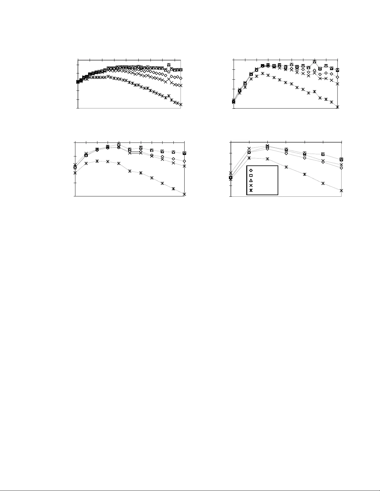
Efficien t Appro ximations for the Margi nal Lik eliho o d of Incomplete Da ta Giv en a Ba y esian Net w ork Da vid Maxw ell Chi c k ering ∗ and Da vid H ec ker man Microsoft Research Redmond W A 98052 -6399 dmax@microso ft.com, heck erma@ micr osoft.com Abstract W e discuss Bayesian methods for learning Bay esia n net works when data sets are incom- plete. In particular, we examine as ymptotic approximations for the marginal likelihoo d of inco mplete data g iven a Bay es ian net- work. W e consider the Laplace approxima- tion a nd the less accura te but more efficien t BIC/MDL approximation. W e also consider approximations prop osed by Drap er (1993) and Cheeseman and Stutz (1995). These ap- proximations are as efficien t as BIC/MDL, but their accuracy has not been studied in any depth. W e compare the a ccuracy o f these approximations under the ass umption that the Laplace a pproximation is the mos t ac- curate. In exp eriments using synthetic data generated f rom discr ete naive-Bay es mo dels having a hidden ro ot no de, w e find that (1) the BIC/MDL meas ur e is the lea st accurate, having a bias in fa vor of simple mo dels, and (2) the Drap er a nd CS measures are the most accurate. 1 In tr o duction There is g rowing interest in metho ds for learning graphical models from data. W e consider Bay es ian methods such as those s ummar ized in Heck er man (1995) a nd Buntine (19 96). A key step in the B ayesian approach to learning graph- ical models is the computation of the marginal likeli- ho o d of a data set given a model. Given a c omplete data set—that is a data s et in which each s ample con- tains observ atio ns for every v a riable in the mo del, the marginal lik eliho o d c a n b e co mputed exactly and ef- ficien tly under certain assumptions (e.g., see Co op er ∗ Author’s p rimary affiliation: Computer Science De- partment, Universit y of California, Los Angeles, CA 90024. & Hersko vits, 199 2; Hec kerman & Geiger, 1995). In contrast, when observ atio ns are missing, including sit- uations where s ome v ar iables a re hidd en or never ob- served, the exact determination o f the ma rginal likeli- ho o d is typically intractable. Conseq uently , approx- imate techn iques for computing the marginal lik eli- ho o d are used. These techni ques include Mo n te Carlo approaches suc h as Gibbs sa mpling and importa nce sampling (Neal, 1993 ; Madigan & Ra ftery , 1 994), se- quent ial up dating methods (Spiegelhalter & Lauritzen, 1990; Cowell, Dawid, & Sebastiani, 19 95), and asymp- totic a pproximations (Kass, Tierney , & Kada ne, 198 8; Kass & Raftery , 199 5; Drap er, 1993 ). In this pap er , we examine a s ymptotic approximations, comparing their accura cy and efficiency . W e con- sider the Lapla c e approximation (Kas s et al., 19 88; Kass & Raftery , 1 995; Azevedo-Filho & Shach ter, 1994) a nd the Bay es ia n Infor mation Criterion (BIC) (Sc h warz, 1978), which is eq uiv a lent to Risannen’s (1987) Minim um-Description-Length (MDL) mea sure. In addition, we consider approximations describ ed by Drap er (1 993) and Cheese ma n and Stutz (1995 ). Both theor etical a nd empirical studies ha ve sho wn that the Laplace appr oximation is mo re ac c ur ate than is BIC/MDL (see, e.g., Draper, 1 9 93, and Raftery , 1994). F urthermore, it is well known that the Laplace approximation is sig nificantly less efficient than are the BIC/MDL, Drap er, and Cheesema n-Stutz mea- sures. T o our knowledge, how ever, there have b een no theoretical or for mal empirical studies that co m- pare the acc ur acy o f the Laplace approximation with those of Drap er and Cheeseman a nd Stutz. W e de- scrib e an exp erimental comparison o f the approxima- tions for learning directed gr a phical mo dels (Bay esia n net works) for discrete v ariables wher e one v a riable is hidden. 2 Bac kground and Motiv ation The Bay esia n appr oach for learning Bay es ian netw o rks from data is as follows. Given a domain or set of v ariables X = { X 1 , . . . , X n } , supp ose we know t hat the true jo in t distribution of X can be encoded in the Bay esian-netw or k structure S . Let S h denote the h yp othesis that this enco ding is p ossible. Also, sup- po se that w e are uncertain ab out the parameters of the Bayesian netw ork ( θ s , a column vector) that de- termine the true joint distribution. Given a prior dis- tribution ov er these par a meters and a random sample (data set) D = { X 1 = x 1 , . . . , X N = x N } fro m the true jo int distribution, w e can a pply Bay es’ rule to infer the p o s terior distribution of θ s : p ( θ s | D , S h ) = c p ( D | θ s , S h ) p ( θ s | S h ) (1) where c is a no rmalization consta nt. Because D is a random s ample, the lik eliho o d p ( D | θ s , S h ) is simply the pr o duct of the individual likelihoo ds p ( D | θ s , S h ) = N Y l =1 p ( x l | θ s , S h ) Given some quan tit y o f interest that is a function of the netw o rk-structure hypothesis and its para meter s, f ( S h , θ s ), w e can compute it s expectation, given D , as fo llows: E ( f ( S h , θ s ) | D, S h ) = Z f ( S h , θ s ) p ( θ s | D , S h ) d θ s (2) Consider the case where the v ariables X are discrete. Let P a i denote the set of v ariables corresp onding to the par ent s of X i . Let x k i and pa j i denote the k th po ssible sta te of X i and the j th p ossible state o f P a i , resp ectively . Also, let r i and q i denote the num b er of po ssible states of X i and P a i , resp ectively . Assuming that there are no logical constr aints on the true joint probabilities other than thos e imp osed by the netw ork structure S , the parameters θ s corresp ond to the true probabilities (i.e., long-run frac tio ns) asso cia ted with the Ba yesian-netw or k s tructure. In particular, θ s is the set of parameters θ ijk for all p ossible v a lues of i, j, and k , where θ ijk is the true pr o bability that X i = x k i given P a i = pa j i . W e use the notation θ ij = ( θ ijk ) r i k =1 θ i = ( θ ij ) q i j =1 θ s = ( θ i ) n i =1 The likelihoo d for a random sample with no missing observ ations is given by p ( D | θ s , S h ) = n Y i =1 q i Y j =1 r i Y k =1 θ N ijk ijk where N ijk are the sufficient statistics for the likelih o o d—the num b er o f samples in D in which X i = x k i and P a i = pa j i . Consequently , we can c o mpute the po sterior distribution of θ s using Equa tion 1. This computation is esp ecially simple when (1) the par am- eter sets θ ij are m utually indep endent—an assump- tion we call p ar ameter indep endenc e —and (2) the prior distribution for each pa rameter set θ ij is a Dirichlet distribution p ( θ ij | S h ) = c r i Y k =1 θ α ijk − 1 ijk (3) where c is a no rmalization constant and the α ijk > 0 may depend on the netw ork structure S . Making the problem more difficult, supp ose that we are also uncer tain ab out whic h structure enco des the true distribution. Given a prior distribution over the po ssible net work-structure hypo theses, w e can com- pute the corr esp onding posterio r distribution using Bay es r ule: p ( S h | D ) = c p ( S h ) p ( D | S h ) (4) = c p ( S h ) Z p ( D | θ s , S h ) p ( θ s | S h ) d θ s Given some qua nt it y of in terest, f ( S h , θ s ), we can compute its exp ectation, given D : E ( f ( S h , θ s ) | D ) = X S h p ( S h | D ) Z f ( S h , θ s ) p ( θ s | D , S h ) d θ s This Bayesian approach is an example of what s ta tisti- cians call mo del aver aging . The key computation here is that o f p ( D | S h ), kno wn as t he m ar ginal likeliho o d of D given S , or simply the margina l likeliho o d of S . In the remainder of the paper, we assume that prior s ov er net work structure are uniform, so that relative po sterior probability and marginal likelih o o d are the same. When we can no t use prior knowledge to restrict the set of p ossible net work structures to a manageable n um b e r , we can select (typically) one mo del S and use Equation 2 to approximate the true exp ectation of f ( S h , θ s ). This approximation is an example of mo del sele ction. In practice, one selects a mo del b y using some searc h pro cedur e tha t pro duces candidate net- work s tructures, applying a sc oring function to each found structure, and retaining the structure with the highest score. One reaso nable sco ring function is the log marginal likelihoo d: log p ( D | S h ). Dawid (1984) no tes the following interesting interpre- tation o f the log mar ginal likelihoo d as a scoring func- tion. Suppo se we use a model S to predict the prob- abilit y of ea ch sample in D given the previously o b- served samples in D , and assig n a utility to each pr e- diction using the log proper scoring rule. The util- it y for the fir st prediction will b e log p ( x 1 | S h ). W e make this prediction based solely on the prior distri- bution for θ s . The utility f or the second prediction will be log p ( x 2 | x 1 , S h ). W e compute this prediction b y training the net work s tructure using only the firs t sample in D . The u tilit y for the i th prediction will be log p ( x i | x 1 , . . . , x i − 1 , S h ). W e make this prediction b y training the net work str ucture with the fir st i − 1 samples in D . Summing these utilities (a s one does with this pro p e r sco ring rule), we obtain N X i =1 log p ( x i | x 1 , . . . , x i − 1 , S h ) By Bay es’ r ule this sum is equal to the log marginal likelih o o d log p ( D | S h ), a nd is indep endent o f the or- der in which we pro ces s the samples in D . Th us, the net work structure with the highest log marginal likeli - ho o d is precisely the mo del that is the b est sequential predictor of the da ta D according to the log sc o ring rule. When the random sample D is co mplete, parameter s are indep endent, a nd para meter priors are Dirichlet, the computation of the marg inal likelihoo d is s traight- forward: p ( D | S h ) = n Y i =1 q i Y j =1 Γ( α ij ) Γ( α ij + N ij ) · r i Y k =1 Γ( α ijk + N ijk ) Γ( α ijk ) (5) This form ula w as first deriv ed by Coo p er and Her- sko vits (1992). Heck erma n et al. (1995) refer to this formula in co njunction with the structure prior as the B ayesian D ir ichlet (BD) s c o ring function. When the r andom s a mple D is incomplete, the exact computation of the ma r ginal likelihoo d is intractable for real-world pro blems (e.g., see Co op er & Hersko vits, 1992). Thus, approximations are required. In this pap er, we consider asy mptotic approximations. One well-known a symptotic approximation is the L aplac e o r Gaussian approximation (Kass et al., 198 8; Kass & Raftery , 1 995; Azevedo-Filho & Shach ter, 1994). The idea b ehind the Laplace a pproximation is that, for larg e a mo un ts of data, p ( θ s | D , S h ) ∝ p ( D | θ s , S h ) · p ( θ s | S h ) ca n o ften b e approximated as a multiv ar ia te Gaussia n distribution. Consequently , p ( D | S h ) = Z p ( D | θ s , S h ) p ( θ s | S h ) d θ s (6) can b e ev alua ted in closed form. In par ticular, let g ( θ s ) ≡ lo g( p ( D | θ s , S h ) · p ( θ s | S h )) Let ˜ θ s be the (vector) v alue of θ s for which the po ste- rior pro bability o f θ s is a ma ximu m: ˜ θ s = ar g max θ s  p ( θ s | D , S h )  = ar g max θ s { g ( θ s ) } The quantit y ˜ θ s is known a s the maxim um a p osteri- ori probability (MAP) v alue of θ s . Expanding g ( θ s ) ab out ˜ θ s , we o btain g ( θ s ) ≈ g ( ˜ θ s ) + − 1 2 ( θ s − ˜ θ s ) t A ( θ s − ˜ θ s ) (7) where ( θ s − ˜ θ s ) t is the transpo se of column v ector ( θ s − ˜ θ s ), and A is the nega tive Hessian of g ( θ s ) ev al- uated a t ˜ θ s . Substituting Equa tion 7 into Equa tion 6, in tegrating, and taking the logarithm of the result, we obtain the Lapla ce appr oximation: log p ( D | S h ) ≈ log p ( D | ˜ θ s , S h ) + log p ( ˜ θ s | S h ) + d 2 log(2 π ) − 1 2 log | A | (8) where d is the dimension of the m o del S giv en D in the region o f ˜ θ s . F o r a Bayesian net work with discr ete v ariables, this dimension is typically the num b er of parameters o f the net work str uctur e , P n i =1 q i ( r i − 1 ). (When enough da ta ar e missing—for example, when one or more v aria bles a re hidden—it may b e that the dimension is low er. See Geiger et al. in this pro cee d- ings for a discussion.) Kass et al. (1988 ) hav e shown that, under certain regularity conditions, error s in this approximation are bounded by O (1 / N ), where N is the num b er of sa mples in D . A more efficient but less ac c urate approximation is ob- tained by retaining only those ter ms in Eq ua tion 8 that increase with N : log p ( D | ˜ θ s , S h ), whic h increases lin- early with N , and log | A | , which increa ses a s d log N . Also, for larg e N , ˜ θ s can b e appr oximated by the max- imum likeliho o d (ML) v alue o f θ s , ˆ θ s , the vector v alue of θ s for whic h p ( D | θ s , S h ) is a maximum. Thus, we obtain log p ( D | S h ) ≈ lo g p ( D | ˆ θ s , S h ) − d 2 log N (9) This a pproximation is called the Bayesia n informa- tion criterion (BIC), and was first derived by Sch warz (1978). Given r egularity conditions similar to those for the Laplace approximation, BIC is a c c ur ate to O (1). That is, for lar g e N , the erro r b ounds of the approximation do not increase as N increases. 1 Thu s, if we use BIC to select one of a set o f mo dels, we will select a mo del whose pos terior probability is a maximum, when N 1 Under some conditions, th e BIC is accurate to O ( N − 1 / 2 ) (Kass & W asserman, 1996). These conditions do not apply to the models we examine in our exp eriments. beco mes sufficien tly large. W e say that BIC is asymp- totic al ly c orr e ct . By this definiti on, the Lapla ce ap- proximation is a lso asymptotica lly cor rect. The BIC approximation is in teresting in several re- sp e c ts. First, it do es not dep end on the prior . Con- sequently , we can use the a pproximation without as - sessing a prio r. 2 Second, the approximation is quite in tuitiv e. Namely , it contains a term measuring ho w well the mo del w ith parameters s et to a n ML v a lue pre- dicts the data (log p ( D | ˆ θ s , S h )) and a term that pun- ishes the complexity of the model ( d/ 2 log N ). Third, the B IC approximation is exactly the additive inv er se of the Minim um Description Length (MDL) scoring function descr ib e d by Rissa nen (198 7 ). Drap er (1993) s uggests another a pproximation to Equation 8, in which the term d 2 log(2 π ) is reta ined: log p ( D | S h ) ≈ lo g p ( D | ˆ θ s , S h ) − d 2 log N + d 2 log(2 π ) (10) This measur e is asymptotically co rrect under the same conditions as those for BIC/MDL. F or finite data s ets, how ever, Drap er (199 3) mentions that he has found his approximation to b e b etter than B IC/MDL. W e shall refer to Equa tion 10 as the Dr ap er scor ing function. T o co mpute the Lapla ce approximation, we must com- pute the neg ative Hessian of g ( θ s ) ev aluated a t ˜ θ s . Meng and Rubin (199 1) describ e a numerical tec h- nique for co mputing the seco nd deriv atives. Raftery (1995) sho ws ho w t o appro ximate the Hessian using likelih o o d-ratio tests that are av ailable in many sta- tistical pac k a ges. Thiesson (19 95) demonstrates that, for discre te v ar iables, the seco nd deriv a tiv es can be computed using Bayesian-net work inference. When computing a ny of these a pproximations, we m ust determine ˜ θ s or ˆ θ s . One technique for finding a maximum is gradient a scent, where we follow the deriv atives of g ( θ s ) or the likelihoo d to a lo cal max- im um. Bun tine (199 4), Russell et al. (1995), a nd Thiesson (1995 ) discuss how to compute der iv atives of the likelihoo d for a Bay esian netw o rk with discr e te v ariables. A more efficien t technique for ident ifying a loc al MAP or ML v alue o f θ s is the EM a lgorithm (Dempster, Laird, & Rubin, 197 7). Applied to B ay esian net works for discr ete v ariables, the E M algo rithm works a s fol- lows. First, we ass ign v alues to θ s somehow (e.g ., at random). Next, we compute the exp e cte d sufficient 2 One of the tec h nical assumptions u sed to derive this appro ximation is that the p rior be n on-zero around ˆ θ s . statistics for the missing entries in the data: E ( N ijk | θ s , S h ) = N X l =1 p ( x k i , pa j i | x l , θ s , S h ) (11) When X i and all the v aria bles in P a i are obser ved in sample x l , the term for this sa mple re q uires a trivial computation: it is either zer o or one. Otherwise, we can use an y Bayesian netw ork infere nce algorithm to ev aluate the ter m. This co mputation is ca lled the E step of the EM alg orithm. Next, we use the exp ected sufficient statistics as if they were ac tua l s ufficien t statistics from a complete r an- dom sample D 0 . If w e are doing a MAP calc ula tion, we compute the v alues of θ s that ma ximize p ( θ s | D 0 , S h ): θ ijk = E ( N ijk | θ s ) + α ijk − 1 E ( N ij | θ s ) + α ij − r i If w e are doing an ML calcula tion, we c o mpute the v alues o f θ s that ma ximize p ( D 0 | θ s , S h ): θ ijk = E ( N ijk | θ s ) E ( N ij | θ s ) This assignment is called the M step of the E M al- gorithm. Dempster et al. (1977) showed that, under certain re g ularity conditions, iteration of the E a nd M steps will conv erg e to a lo cal ma ximum . The EM alg o- rithm a s sumes parameter indep endence, 3 and is typ- ically used whenev e r the ex pected sufficient statistics can be computed efficiently (e.g., discrete, Gaussian, and Gauss ian-mixture distr ibutions). In the E M algorithm, we treat expected sufficient statistics as if they are a c tua l sufficient statistics. This use s uggests a nother approximation for the marginal likelih o o d: log p ( D | S h ) ≈ lo g p ( D 0 | S h ) (12) where D 0 is an imaginary data set that is co nsistent with the exp ected sufficient statistics computed using an E step at a lo ca l ML v a lue for θ s . F or discrete v ariables, this approximation is giv en b y the logar ithm of the right-hand-side of Equation 5, where N ijk is replaced by E ( N ijk | ˆ θ s ). W e ca ll this scor ing function the mar ginal likeliho o d of the ex p e cte d data o r MLED. MLED has tw o desirable prop er ties. One, be- cause it computes a marginal likelihoo d, it punishes mo del complexity as does the La place, Draper, and BIC/MDL measures. Two, beca us e D 0 is a complete (albe it imaginary) data set, the computation of the measure is efficient. 3 Actually , some parameter sets ma y b e equal, provided these sets are mutually ind ep endent. One pro blem with this scor ing function is that it may not be asymptotically correct. In particular, as suming the B IC / MDL reg ularity conditions apply , we hav e log p ( D 0 | S h ) = lo g p ( D 0 | ˆ θ s , S h ) − d 0 2 log N + O (1) where d 0 is the dimension of the model S given data D 0 in the region a round ˆ θ s —that is, the num b er o f pa - rameters of S . As N increases, the difference b etw een p ( D | ˆ θ s , S h ) and p ( D 0 | ˆ θ s , S h ) may increas e. Also , a s we hav e d iscussed, it ma y be that d 0 > d . In either case, MLED will not be as ymptotically co rrect. A sim- ple mo dification to MLE D address es these problems: log p ( D | S h ) ≈ log p ( D 0 | S h ) (13) − log p ( D 0 | ˆ θ s , S h ) + d 0 2 log N + log p ( D | ˆ θ s , S h ) − d 2 log N Equation 12 (without the cor rection to dimension) was firs t prop osed by Chee s eman and Stutz (199 5) as a scoring function for AutoClass, an algo r ithm for data clustering. W e shall refer to Equation 13 as the Che eseman-S tutz (CS) scor ing function. W e note that bo th the MLED and CS scoring functions can easily be extended to the directed Gaussia n-mixture mod- els describ ed in La uritzen and W ermut h (198 9 ) and to undirected Gaussian-mixture mo dels. The accura cy of these approximations, w hich w e ex- amine in the following tw o sections, must b e balanced against their co mputation co s ts. The ev alua tio n of CS, MLED, Drap er, and BIC/MDL is dominated by the determination of the MAP or ML. The time complex- it y of this task is O ( edN i ), where e is the n umber o f EM iterations and i is the cost of inference in Equa- tion 11 . The ev aluation of the La place approximation is do minated by the computation of the determinant of the nega tive Hessian A . The time co mplexity of this computation (using Thiesson’s 1995 metho d) is O ( d 2 N i + d 3 ). T y pica lly e < d and d < N so that the Laplace a ppr oximation is the least efficien t, ha v- ing co mplexity O ( d 2 N i ). 3 Exp erimen tal Design As mentioned, the La place appr oximation is known to be more accurate than the BIC/ MDL and Drap er ap- proximations. In contrast, to our k nowledge, no the- oretical (or empirical) work has b een done co mpa ring the Laplace approximation with the CS or MLE D ap- proximations. Nonetheless, in our e x per iment s, we as- sume that the Laplace approxim ation is the mos t accu- rate of the approximations, and meas ur e the a ccuracy of the o ther approximations using the Laplace approx- imation as a gold s tandard. W e c a n not verify our as - sumption, b eca use exact computations of the ma rginal likelih o o d ar e not p ossible for the mo dels that we con- sider. Thus, th e results of our experiments m ust b e in terpreted with caution. In particular, w e c a n not rule out the p os sibilit y that the CS o r MLED approx- imations a re b etter than the Laplace approximation. W e ev aluated the accuracy of the CS, MLED, Drap er, and BIC/MDL appr oximations relative to that of the Laplace approximation using syn thetic mo dels con- taining a single hidden v ar iable. F or r easons discusse d in Section 4, we limited our synthetic net works to naive-Ba yes mo dels for discrete v ariables (also known as disc r ete mixture mo dels). A naive-Ba yes mo del for v ariables { C, X 1 , . . . , X n } enco des the assertion that X 1 , . . . , X n are m utually independent, given C . The net work structure for this model co nt ains the single ro ot no de C and leaf no des X i each having only C as a parent. (W e use the same notation to refer to a v ari- able a nd its corr esp onding no de in the netw o rk struc- ture.) W e generated a v ar iety of naive-Ba yes mo d- els by v arying the num b er of sta tes of C ( c ) and the n um b e r of obs e r ved v a r iables n (all of whic h are bi- nary). W e determined the para meters of each mo del b y sa mpling from the uniform (Dirichlet) distribution ( α ijk = 1). W e sa mpled data from a model so as to make the ro ot no de C a hidden v a riable. Namely , we sampled data from a mo del using the usual Monte-Carlo approach where we first sa mpled a sta te C = c according to p ( C ) a nd then sa mpled a s ta te o f each X i according to p ( X i | C = c ). W e then discarded the samples of C , retaining only the samples of X 1 , . . . , X n . In a single exp e riment , we first genera ted a mo del for a given n and c , and subsequently five data sets for a given sample size N . Next, we appr oximated the marginal lik eliho o d for each data set given a ser ies of test mo dels that were identical to the synthesized mo del, ex cept we allow ed the n um be r of states of the hidden v ariable to v ar y . Finally , we compar ed the dif- ferent appr oximations of the marginal likelih o o d in the context of b oth mo del a veraging a nd mo del selection. T o compare the a pproximations for mo del a veraging , we s imply co mpared plots o f lo g margina l likelih o o d versus states o f the hidden v ar iable in the test mo del directly . T o compare the approximations for model selection, we co mpa red the n umber of sta tes of the hidden v ar ia ble selected using a given approximation with the num b er of states selected using the Laplace approximation. W e initialized the EM algo r ithm a s follows. Fir st, we initialized 64 copies of the par ameters θ s at random, - 2 2 0 0 - 2 1 5 0 - 2 1 0 0 - 2 0 5 0 - 2 0 0 0 - 1 9 5 0 - 1 9 0 0 2 3 4 5 6 7 8 - 4 0 5 0 - 4 0 0 0 - 3 9 5 0 - 3 9 0 0 - 3 8 5 0 - 3 8 0 0 - 3 7 5 0 2 3 4 5 6 7 8 - 7 3 0 0 - 7 2 0 0 - 7 1 0 0 - 7 0 0 0 - 6 9 0 0 - 6 8 0 0 2 3 4 5 6 7 8 - 1 3 8 0 0 - 1 3 6 0 0 - 1 3 4 0 0 - 1 3 2 0 0 - 1 3 0 0 0 - 1 2 8 0 0 2 3 4 5 6 7 8 - 2 2 0 0 - 2 1 5 0 - 2 1 0 0 - 2 0 5 0 - 2 0 0 0 - 1 9 5 0 - 1 9 0 0 2 3 4 5 6 7 8 n = 8 n = 16 n = 32 n = 64 La P l a c e C S M L E D D r a p e r B I C / M D L Figure 1: Approximate log marg inal likelihoo d of the da ta giv en a test mo del as a function o f the num b er o f hidden states in the test mo del. The 4 00 sample data sets were generated from naive-Bay es mo dels with n observed v a riables and 4 hidden states. and ra n one E and M step. Then, w e retained the 32 copies of the para meters for which g ( θ s ) was lar gest, and ran tw o EM iterations. Next, we re ta ined the 16 copies of the para meters for which g ( θ s ) was lar gest, and ran 4 EM iteratio ns. W e contin ued this pro ce- dure four mo re times, until only one set o f par ameters remained. T o guarantee conv ergence of the EM alg orithm, we per formed 200 E M iterations following the initializa- tion phase. T o c heck that the alg o rithm had co n- verged, w e meas ur ed the relative change of g ( θ s ) b e- t ween successive iterations. Using a conv e rgence crite- rion s imila r to that of AutoCla s s’ default, we said that the EM algo r ithm had conv er ged when this relative change fell b elow 0.00 001. The alg o rithm conv erg ed in a ll but one of the 550 r uns. W e assig ned Dirichlet priors to each parameter set θ ij . W e used the almost uniform prior α ijk = 1 +  , b ecaus e it pro duced lo cal maxima in the interior of the para m- eter spa ce. (The traditional Laplace approximation is not v alid at the b oundar y of a parameter space.) Our conclusions are not s ensitive to  in the range we tested (0.1 to 0.001). W e rep ort results for the v a lue  = 0 . 0 1. As desc r ib e d by Equation 8 , we ev alua ted the Laplace approximation at the MAP of θ s . T o simplify the com- putations, we also ev aluated the CS, MLED, Drap er, and BIC/ MDL measur es at the MAP . Giv e n our choice for α ijk , the differences b etw een the MAP and ML v al- ues were insignificant. W e used the metho d of Thies- son (1995 ) to ev a luate the negative Hessian of g ( θ s ). T o compute the CS scor ing function, we ass umed that dimensions d 0 and d are equal. Although we hav e no pro of of this assumption, exp eriments in Geiger et al. (in this pro ceedings) sugg e st that the assumption is v alid. All exp eriments were run o n a P5 100MHz machine under the Windows NT TM op erating system. The a l- gorithms were implemented in C++. 4 Results and Discussion First, we ev aluated the approximations for use in mo del av era g ing, comparing plots of approximate log marginal likelihoo d versus the n um ber of s ta tes o f the hidden v ar iable in the test mo del. W e conducted three sets of compa risons for differen t v a lues of c (num b er of states of the hidden v a riable), n (n umber of ob- served v aria bles ), and N (sample size). The results are almost the s ame for different data s ets in a g iven exp e riment (if we were to show one- standard devia- tion error s bars, they would b e invisible for most data po int s, a nd ba rely visible for the r emaining p oints). Consequently , we show re sults fo r only o ne da ta set - 2 0 5 0 0 - 1 9 5 0 0 - 1 8 5 0 0 - 1 7 5 0 0 - 1 6 5 0 0 - 1 5 5 0 0 2 6 1 0 1 4 1 8 2 2 2 6 3 0 3 4 - 1 7 0 0 0 - 1 6 5 0 0 - 1 6 0 0 0 - 1 5 5 0 0 - 1 5 0 0 0 - 1 4 5 0 0 2 4 6 8 1 0 1 2 1 4 1 6 1 8 2 0 - 1 3 8 0 0 - 1 3 6 0 0 - 1 3 4 0 0 - 1 3 2 0 0 - 1 3 0 0 0 - 1 2 8 0 0 2 3 4 5 6 7 8 - 1 6 0 0 0 - 1 5 6 0 0 - 1 5 2 0 0 - 1 4 8 0 0 - 1 4 4 0 0 4 5 6 7 8 9 1 0 1 1 1 2 1 3 1 4 c = 3 2 c = 1 6 c = 8 c = 4 L a P l a c e C S M L E D D r a p e r B I C / M D L Figure 2: Approximate log marg inal likelihoo d of the da ta giv en a test mo del as a function o f the num b er o f hidden states in the test mo del. The 400 sa mple data sets were generated from naive-Bay es models with 6 4 observed v a riables and c hidden states. per experiment. In our first set o f exp eriments, w e fixed c = 4 and N = 400 and v ar ie d n . In particular, we generated 400-sa mple data sets from four naive-Bay es mo dels with 8, 16, 32, and 64 observed v a riables, r esp ectively , each mo del having a hidden v a riable with four states. Figure 1 shows the approximate log marginal likeli- ho o d of a data g iven test mo dels having hidden v ari- ables with t wo to eight states. (Recall tha t each test mo del has the same num b er of observed v ariables as the co rresp onding g enerative model.) In our sec o nd s e t of exp eriments, w e fixed n = 64 and N = 400, and v aried c . In par ticular, we gener- ated 400 -sample data sets from four naive-Bay es mo d- els with c = 32 , 1 6, 8 , a nd 4 hidden states re s pec tively , each mo del ha ving 64 o bserved v a r iables. Figure 2 shows the approximate log marginal lik e liho od of a data for test models having v alues of c that straddle the v a lue of c for the generative mo del. In our third s et of exp eriments, w e fixed n = 32 a nd c = 4, and v aried N . In particular, from a naive- Bay es mo del with n = 32 and c = 4, w e generated data sets with sample sizes ( N ) 1 00, 200, 400, and 800, r e s pec tiv ely . Figure 3 shows the a ppr oximate log marginal likelihoo d o f a data for test mo dels having hidden v ar iables with tw o to eight states. The trends in the marg inal-likelihoo d curves a s a func- tion of n , c , a nd N a re not sur prising. F or each ap- proximation, the curves b ecome more p eaked ab o ut the v alue of c (the num b er of hidden states in the gen- erative mo del) as (1) N increa s es, (2) n increa ses, and (3) as c decreases. The first result says that learning improv es as the amount o f data increases. The second result is a r eflection of the fact that large r num b ers of observed v ar iables provide mor e evidence for the iden- tit y of the hidden v ariable. The third res ult says that it b ecomes mo r e difficult to lear n a s the num b er o f hidden sta tes increa ses. In comparing these curves, note that only differences in the shap e of the curves ar e impor tant. The heigh t of the curves are not imp or ta n t, bec ause the ma r ginal likelih o o ds (i.e., rela tive poster io r pr obabilities) ar e normalized in the pro cess of mo del av erag ing. Over- all, the Draper and CS scoring functions appea r to be equally go o d approximations, b oth b etter than the BIC/MDL. The MLED and CS scoring functions are almost identical, except for small v alues of n , wher e the CS a pproximation is b etter. Next, we e v a luated the appr oximations for use in mo del selection. In each exper imen t for a particular n , c , a nd N , we computed the size o f the mo del se- lected by a given approximation—that is, the num b er of states of the hidden v ar iable in the test mo del hav- - 2 1 0 0 - 2 0 0 0 - 1 9 0 0 - 1 8 0 0 - 1 7 0 0 - 1 6 0 0 2 3 4 5 6 7 8 - 3 9 0 0 - 3 8 0 0 - 3 7 0 0 - 3 6 0 0 - 3 5 0 0 - 3 4 0 0 2 3 4 5 6 7 8 - 7 3 0 0 - 7 2 0 0 - 7 1 0 0 - 7 0 0 0 - 6 9 0 0 - 6 8 0 0 2 3 4 5 6 7 8 - 1 4 1 0 0 - 1 4 0 0 0 - 1 3 9 0 0 - 1 3 8 0 0 - 1 3 7 0 0 - 1 3 6 0 0 - 1 3 5 0 0 2 3 4 5 6 7 8 N = 10 0 N = 20 0 N = 40 0 N = 80 0 La P l a c e C S M L E D D r a p e r B I C / M D L Figure 3 : Approximate log marginal likelihoo d o f the data given a test mo del as a function of the num b er of hidden states in the test mo del. The da ta sets of size N w ere generated fro m na ive-Ba yes models with 32 observed v a riables and 4 hidden states. ing the la rgest approximate marginal lik eliho o d. W e then subtracted fro m this num b er the size of the mo del selected by the g old-standard La place a pproximation, yielding a quantit y called ∆ c . The res ults a r e shown in T a ble 1. Overall, the Dra pe r , CS, and MLED sco ring functions are more accurate than the BIC/MDL, whic h consis - ten tly sele c ts mo dels that are to o simple. The CS and MLED results are almost the same, exc e pt for s mall v alues of n where CS do es slig h tly better. The CS a nd MLED mea sures tend to select mo dels that ar e to o complex (∆ c > 0), wher eas the Drap er measure tends to select mo dels that are to o simple (∆ c < 0). F or large v a lues of c , the Drap er measure do es b et- ter than the CS a pproximation for lar ge v alues of c . The sourc e of this difference ca n b e seen in the top t wo gr aphs of Figure 2. All algorithms in both these graphs show t wo p eaks: a br oad pe a k aro und c/ 2 and a sha r p pe a k ar ound c , where c is the n umber of hid- den states in the gener ative mo del. The Laplace and Drap er (and BIC) curves tend down ward o n the right sharply enough s uch that the first pea k dominates. In contrast, the CS curve remains fairly flat to the right such that the second p eak dominates. The existence of the second p e a k a t the true nu mber of hidden states is quite in teresting (and unexpected), but we do not pursue it further in this pap er. As we have discuss e d, the accurac y results must b e balanced against the computational costs of the v a r- ious appr oximations. The time complexities g iven in Section 2 are overly p ess imistic for naive-Bay es mo d- els, b ecause probabilistic inferences can b e ca ched and reused. F or naive-Bay es mo dels, the ev aluation of the CS, MLE D, Dra p er , and B IC/MDL mea sures (a g ain dominated by the MAP computation) has time com- plexit y O ( edN ). The ev aluation o f Laplace a pproxi- mation (again dominated by the determina tio n of the Hessian), is given by O ( d 2 N ). T o a ppreciate the co n- stants for these cos ts, the run times for the e x per iment n = 64 , c = 3 2 , N = 4 00 are shown in T able 2. The b ottom line is that the Drap er a nd CS measures are bo th accurate and efficien t, and are probably the approximations o f choice for most applications. Our findings a re v alid o nly for naive-Ba yes models with a hidden r o ot no de. These results a re imp orta n t, be- cause they apply directly to the AutoClass alg o rithm, which is g rowing in p opularity . Also , it is likely that our results will extend to mo dels for discrete v a r iables and data sets where each v ar iable that is uno bserved has an observed Marko v blanket. Under these condi- tions, each Bay esia n inference required by the scoring functions (e.g., Equa tion 1 1) reduces to a na ive-Ba yes computation. Nonetheless, mo r e detailed exp eriments are warranted to address mo dels with more general T able 1 : E rror s in mo del selection (mean ± s.d.). Exp eriment ∆ c n c N CS MLED Drap er B IC/MDL 8 4 400 0 0.4 ± 1.5 0 -0.2 ± 0 .4 16 4 400 0.2 ± 0.4 -0.2 ± 0 .8 0.2 ± 0.4 -0.8 ± 0 .4 32 4 400 0 0 0 -0.4 ± 0 .5 64 4 400 0 0 0 -0.2 ± 0 .4 64 32 400 16 .2 ± 1.5 16.2 ± 1.5 -2.2 ± 2.0 -6.0 ± 2.7 64 16 400 5.0 ± 6.4 5.0 ± 6.4 -1.6 ± 1.1 -3.0 ± 1.4 64 8 400 0.8 ± 0.8 0.8 ± 0 .8 0 -1.0 ± 1 .0 64 4 400 0 0 0 -0.2 ± 0 .4 32 4 100 0.6 ± 0.9 0 .6 ± 0.9 0 - 0.6 ± 0.5 32 4 200 0.2 ± 0.4 0 .2 ± 0.4 0 - 0.6 ± 0.5 32 4 400 0 0 0 -0.4 ± 0 .5 32 4 800 0 0 0 0 structure a nd non-discrete distributions. Finally , we again note that our results do not rule out the p ossi- bilit y that the CS or MLED approximations are b etter than the La place approximation. 5 Realit y Check In o ur analysis o f s coring functions for hidden-v ariable mo dels, w e ha ve made an impo r tant as sumption. Namely , we hav e ass umed that, when the true model contains a hidden v ariable, it is b etter to learn b y searching o ver models with hidden v ar iables than those without hidden v ariables . This assumption is not triv- ially cor rect. Given a na ive-Ba yes mo del for the v ari- ables C, X 1 , . . . , X n , the join t distribution for these v ariables can b e enco ded b y a Bay es ian net work with- out hidden v a r iables. (Assuming there are no acci- den tal cancellations in the probabilities, this Bay esia n net work will be completely connected.) Thus, we can attempt to learn a mo del containing no hidden v ar i- ables, and this mo del may b e mo re acc ur ate than that learned by searching ov er naive-Bay es mo dels ha ving a hidden ro o t no de. W e tested our a ssumption as follows. First, we gen- erated a naive-Bay es mo del with n = 1 2 and c = 3. F rom this mo del w e generated a data set of size 800, discarding the obser v a tions of the v ariable C . Sec- ond, we lea rned a single naive-Bay es mo del contain- ing a hidden ro ot no de using the exp erimental tech- nique describ ed in the previo us section. In pa rticular, we v aried the num b er of hidden states of the naive- Bay es model, and selected the one with the la rgest (approximate) mar ginal likelihoo d. (In this case, all scoring functions yielded the s ame mo del: one with three hidden states). Third, we lear ned a single mo del containing no hidden v ariables using the approach de- scrib ed in Heck erman et al. (1995 ). In particular, we used the BD scoring function with a uniform prior o ver the pa rameters in conjunction with a gr eedy search al- gorithm (in directed-gra ph spa ce) initialized with an empt y graph. W e e v a luated the tw o lear ned mo dels by comparing their marg inal likelihoo ds. Spec ifica lly , we computed ∆ m ≡ log p ( D | S h hidden ) − log p ( D | S h nohide ). W e used the La place a pproximation to compute the fir st term, and the exact express ion for mar ginal likelihoo d (e.g., Heck erman et al., 1995) to c ompute the second ter m. Repea ting this exp eriment five times, we obtained ∆ m = 26 ± 33, indicating that the hidden-v aria ble mo del better predicted the data. In additional exp er- imen ts, we found that ∆ m incr e a sed as we increase d the s ize of the mo dels. 6 Conclusions W e hav e ev aluated the La place, CS, MLED, Drap er , and BIC/MDL approximations for the mar ginal likeli- ho o d of naiv e-Bay es mo dels with a hidden ro ot no de, under the as sumption that the La place approximation is the mo s t accurate o f the scoring functions. Our exp e riment s indicate that (1) the BIC/MDL mea sure is the least accurate, having a bia s in fav or of simple mo dels, and (2) the Dra per and CS measur es ar e the most accur ate, having a bias in fav or o f s imple and complex mo dels, r esp ectively , in most cases . Ac kno wledgmen ts W e thank Dan Geiger and Chris Meek fo r useful discussions about asymptotic approximations, Ko o s Rommelse for his help with s ystem implemen ta tion, and the anonymous reviewers for their suggestions . T able 2: Algorithm run times (in seconds) as a function of the dimension of the test mo del for the exp eriment n = 64 , c = 3 2 , and N = 400 . The v alues for EM are times to conv ergence. The v alues for the scoring functions exclude EM r un times. d EM La pla ce CS MLED Drap er BIC/MDL 1689 500 2800 2 0.06 2 2 1754 580 3000 2 0.07 2 2 1819 590 3300 2 0.07 2 2 1884 650 3600 2 0.08 2 2 1949 680 3900 2 0.08 2 2 2014 680 4200 2 0.08 2 2 2079 530 4600 2 0.08 2 2 2144 760 4900 2 0.08 2 2 2209 810 5500 2 0.08 2 2 2274 790 5900 3 0.08 3 3 2339 870 6700 3 0.08 3 3 References Azevedo-Filho, A., & Shacht er, R. (1994). Laplace’s method approximations for pro babilistic infer- ence in b elief netw orks with con tin uous v a riables. In de Mantaras, R. L., & Po ole, D. (Eds.), Pr o- c e e dings of T enth Confer enc e on Unc ertainty in Artifici al Intel ligenc e, Sea ttle, W A, pp. 28 –36. Morgan K aufmann, San Mateo, CA. Bunt ine (1 9 96). A guide to the litera ture on learning graphical mo dels . IEEE KDE , t o app e ar . Bunt ine, W. (19 94). Op erations for learning with graphical mo dels. Journal of A rt ificial Intel li- genc e R ese ar ch , 2 , 159–22 5 . Cheeseman, P ., & Stutz, J. (1995). Bay es ia n cla s- sification (AutoClass): Theory and r esults. In F ayy ad, U., P iatesky-Shapiro , G., Smyth, P ., & Uth ur usamy , R. (Eds.), A dvanc es in Know le dge Disc overy and Data Mining , p. ?? AA AI Press, Menlo Park, CA. Co op er, G., & Hersko vits, E. (1992). A Bay esia n method fo r the induction of probabilistic net- works from data. Machine L e arning , 9 , 309–3 47. Cow ell, R., Da wid, A., & Seba stiani, P . (1995). A comparison of s e q uen tial learning methods for incomplete data. T ech. rep. 135, Departmen t of Statistical Science, Universit y College London. Dawid, P . (1984). Present p osition and p otential de- velopmen ts: so me p e r sonal views. statistical the- ory . the prequential appro a ch (with Discussion). Journal of the R oyal St atistic al So ciety A , 147 , 178–2 92. Dempster, A., Lair d, N., & Rubin, D. (1977). Max- im um likelihoo d from incomplete data via the EM algorithm. Journal of the Ro yal Statistic al So ciety , B 39 , 1–38 . Drap er, D. (199 3). Assess men t and propa gation o f mo del uncertaint y . T ech. rep. 124, Departmen t of Statistics, Universit y o f California, Lo s Ange- les. Geiger, D., Heck erman, D., & Meek, C. (1996 ). Asymptotic mo del selection for directed net- works with hidden v ar ia bles. In Pr o c e e dings of Twelfth Confer enc e on Unc ertainty in Artificia l Intel li genc e, P ortland, OR. Morga n Kaufmann. Heck erman, D. (199 5). A tutor ial on learning Bay esian net works. T ech. rep. MSR-TR-95 -06, Micro soft, Redmond, W A. Revised January , 1996. Heck erman, D., & Geiger, D. (1995 ). Likeliho o ds a nd priors for Bay esia n netw or k s. T ech. rep. MSR- TR-95-54 , Micr osoft, Redmond, W A. Heck erman, D., Geiger, D., & Chick ering, D. (199 5). Learning Bayesian netw or k s: The co mbin ation of knowledge and sta tistica l data. Mach ine L e arning , 20 , 1 97–24 3. Kass, R., & Ra ftery , A. (19 9 4). Bayes factors. J ournal of the Americ an St atistic al So ciety , 90 , 773– 795. Kass, R., Tierney , L., & Kadane, J. (19 8 8). Asymp- totics in Bay esian co mputation. In Bernardo, J., DeGro ot, M., Lindley , D., & Smith, A. (Eds.), Bayesia n Statistics 3 , pp. 261– 2 78. Ox fo r d Uni- versit y P r ess. Kass, R., & W asser man, L. (199 6). A reference Bay esia n test for nes ted hypotheses and its re - lationship to the Sch warz criterio n. Biometrika , to app e ar . Lauritzen, S., & W ermuth, N. (1989). Graphical mo d- els for asso ciations b etw een v aria bles, some o f which are qualitative and some quantitativ e. An- nals of Statistics , 17 , 31– 57. Madigan, D., & Raftery , A. (1994 ). Mo del selectio n and accounting for mo del uncer taint y in gra phi- cal mo dels using Occam’s window. Journal of the Ameri c an Statistic al Asso ciation , 89 , 1535 –1546 . Meng, X., & Rubin, D. (1991). Using EM to obtain asymptotic v a r iance-cov a riance matrices: The sem a lgorithm. Journal of the Ameri c an Sta- tistic al Ass o ciation , 86 , 899 –909 . Neal, R. (199 3). P robabilistic inference using Markov chain Monte Carlo metho ds. T e ch. r ep. CRG - TR-93-1, Department of Computer Science , Uni- versit y o f T oro nto. Raftery , A. (199 4). Approximate Bayes factors and accounting for mo del uncertain ty in generalized linear mo dels. T ech. rep. 255 , Department of Statistics, Universit y of W ashington. Raftery , A. (199 5). Bay esian mo del selection in so- cial res earch. In Marsden, P . (Ed.), So ciolo gic al Metho dolo gy . Blac kwells, Cambridge, MA. Rissanen, J. (1987). Sto chastic complexity (with dis- cussion). Journal of the Roy al Statistic al So ciety, Series B , 49 , 223 –239 and 2 53–2 65. Russell, S., Binder , J., Ko ller , D., & Kana z awa, K. (1995). Lo cal learning in probabilistic netw orks with hidden v ar iables. In Pr o c e e dings of the F ourte ent h International Joint Confer enc e on Artifici al Int el ligenc e, Mo n treal, QU, pp. 1146– 1152. Morg an Kaufmann, San Mateo, CA. Sch warz, G. (1 9 78). Estimating the dimension of a mo del. Annals of Statistics , 6 , 461 –464 . Spiegelhalter, D., & Lauritzen, S. (1990). Sequential upda ting of conditional probabilities o n directed graphical s tr uctures. Networks , 20 , 57 9–605 . Thiesson, B. (199 5 ). Sco re and information for recur - sive exp onential mo dels with incomplete data. T ech. rep., Institute of E lectronic Systems, Aal- bo rg Universit y , Aalb org , Denmark.