A multi-resolution, non-parametric, Bayesian framework for identification of spatially-varying model parameters

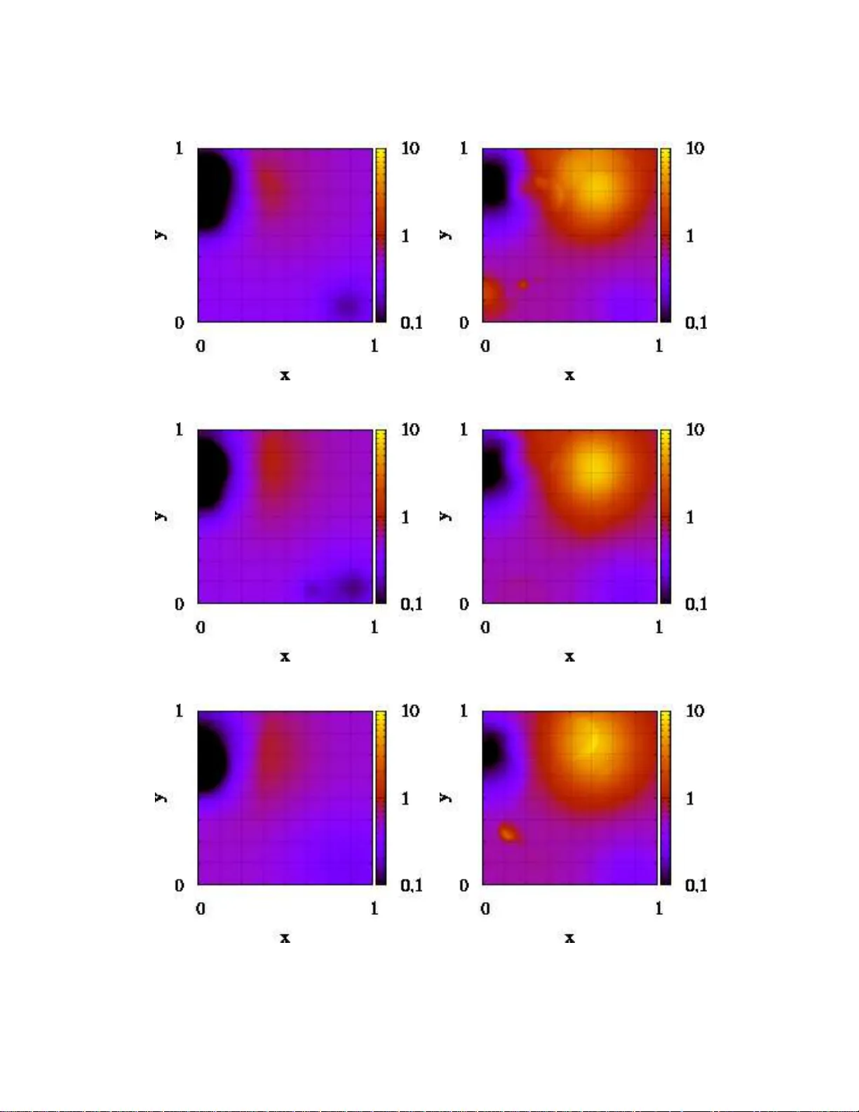
A multi-resolution, non-param etric, Bayesian framework f or identificati on of spatially-varying model param eters. P .S. Koutsour elakis School of Ci v il and Environmental Engineer ing & Center fo r Applied Mathematics Cornell University , Ithaca NY pk285@cornel l.edu Abstract This paper propo ses a hierarchica l, mu lti-resolution fr amew ork for the identifi- cation of mod el p arameters an d th eir spatially variability fro m noisy measure- ments of the respo nse or o utput. Such p arameters are frequently encou ntered in PDE-based mo dels and correspond to quantities such as density or pressure fields, elasto-plastic moduli and intern al variables in solid mechanics, con ductivity fields in heat dif fusion problems, pe rmeability fields in fluid flow th rough porous media etc. T he proposed model has all the advantages of traditional Bayesian formu la- tions suc h as the ability to prod uce measures of c onfidence for the inference s made and providing no t o nly predictive estimates but also quantitative measures of the predictive uncer tainty . In co ntrast to existing approaches it utilizes a parsimo- nious, non -parametr ic form ulation that fav ors sparse represen tations a nd who se complexity can be determ ined from the data. The prop osed framew ork in non- intrusive and makes use of a sequenc e of forward solvers o perating at various resolutions. As a result, inexpensi ve, coarse solvers are used to identif y the most salient featur es of the un known field(s) wh ich are sub sequently enriched by in- voking solvers operating at finer reso lutions. This leads to significant co mpu- tational sa vin gs particularly in pr oblems inv o lving co mputation ally d emanding forward mo dels but also imp rovements in ac curacy . It is based on a novel, ada p- ti ve sch eme based on Seque ntial Monte Carlo samp ling wh ich is embarrassingly parallelizable an d cir cumvents issues with slow mix ing encoun tered in Ma rkov 1 Chain Mo nte Carlo schemes. The cap abilities of the proposed metho dology are illustrated in prob lems fro m n onlinear solid mechan ics with specia l attention to cases where the data is contamina ted with rand om noise and the s cale of variabil- ity of th e unkn own field is smaller than th e scale of the grid whe re obser vations are collected. 1 Intr oduction The prodigious ad vances in computation al modeling o f physical processes and the d e velopment of highly non- linear , mu ltiscale and multiphysics models poses se veral challenges in parameter iden- tification. W e are fr equently using large, forward models which imp ly a significant comp utational burden, in or der to analyze co mplex phenom ena.The extensive u se of such models p oses several challenges in para meter identificatio n as the accu racy of the results provided d epends strongly on as- signing pr oper values to the various mod el parameter s. I n mech anics of materials, accu rate mechan- ical prop erty ide ntification can guide damage detection and an informed assessment of the system’ s reliability ([37]). Identify ing pro perty-cro ss correlations can lead to the design of m ulti-functio nal materials ([62]). In biomechanics, the detection of variations in mechanical properties of human tis- sue can re veal the appearan ce of diseases (arteriosclerosis, malignant tumors) but can also be used to assess the effectivity of various trea tments ([4, 21]). Permeability estimation for soil tra nsport processes can assist in detection of contamina nts, oil explo ration etc. ([68, 23]). W e consider phenomena described by a set of (coupled ) elliptic, par abolic or h yperbo lic PDEs and associated bound ary (and initial) co nditions: A ( y ( x ); f ( x )) = 0 , ∀ x ∈ D (1) where A den otes the differential o perator defined on a do main D ∈ R d , where d is the num ber of spatial dimensions. A d epends on spatially v arying coefficients f ( x ) , x ∈ D . Advances in computatio nal mathematics have g i ven rise to se veral efficient solvers for a wid e-range of suc h systems and have rev olu tionized simulation- based analysis and design ([53]). Our pr imary inter est is to iden tify f ( x ) fro m a set of (po tentially noisy) measurements of the response y i = y ( x i ) at a num ber of d istinct loca tions x i ∈ D . In the case o f time-de pendent PDEs, the av ailab le d ata might also b e indexed by time. Several different processes in so lid and fluid mechanics, transport pheno mena, heat d iffusion etc fall u nder this gen eral setting and even though the co efficients f ( x ) have a different physical interp retation, th e a ssociated inverse problems exhib it similar mathematical characteristics. T wo b asic approach es ha ve been followed in addr essing problems of d ata-driven parametr ic identi- fication. On on e hand, deterministic optimization techniques which attempt to minim ize the sum of the squa res of the deviations betwee n model pre dictions and ob servations. Gr adient or global, in- 2 trusiv e or non-intrusive techn iques are intro duced for performing the optimization task. Usu ally the objective fun ction is augmented with regularization terms (e.g. Tikhonov r egularization [59]) which alleviate issues with the ill-posednesss of th e p roblem ( [60, 27, 19, 64, 5, 38]). Such de terministic in verse tech niques based on exact matching or least-squares optimization, lead to point estimates of unknowns withou t rigo rously con sidering the statistical nature o f system uncerta inties and w ithout providing quantification of the uncertainty in the in verse solution. The dir ect stoch astic cou nterpart of optimization method s inv o lves f requentist appr oaches based on maximu m likelihood estima tors th at aim at m aximizing the p robability of observations giv en the inverse solution m aximum ( [20, 18]) . In recent yea rs significant a ttention has been d irected to- wards statistical appro aches based on the Bayesian paradigm which attempt to calcu late a (posterior) probab ility distribution fu nction on the pa rameters o f inter est. Bayesian form ulations offer several advantages as they provide a un ified fra mew o rk f or d ealing w ith th e u ncertainty intro duced b y the incomplete and no isy measureme nts and assessing quan titati vely re sulting infere ntial uncertainties. Significant successes ha ve bee n no ted in app lications such as medical tomog raphy ([6 9]), geolog ical tomogr aphy ([25, 2]), hy drology ( [44]), p etroleum en gineering ([28, 8]), as well as a host of other physical, biological, or social systems ([42, 57, 67, 48]). Identification of spatially v arying model pa rameters p oses several m odeling and com putational is- sues. Representations o f the parametric fields in existing ap proache s artificially impose a mini- mum length scale of variability usually determin ed by the discretization size of the governing PDEs ([44]). Furthermor e, they are associated with a very large vector o f unknowns. In ference in hig h- dimensiona l spaces using standard optimizatio n or sampling schemes (e.g . Markov Ch ain M onte Carlo (MCMC)), is g enerally impractical as it requ ires an exuberant number of calls to the f orward simulator in or der to achiev e convergence. Particularly in Bayesian formulatio ns wher e the infer- ence results are m uch richer an d inv olve a distribution rather than a single value fo r the para meters of interest, the computational effort imp lied by repeated calls to t he fo rward solver can be enormous and constitute the method impr actical for realistic app lications. T hese p roblems ar e am plified if the p osterior distribution is multi-mod al i.e. se veral sig nificantly different scena ria are likely g i ven the av ailable data. While it is a pparent that, comp utationally inexpensive, c oarser scale simulatio ns can assist the identification process ( [14]), the critical task of effi ciently transferring the informa- tion a cross resolu tions still r emains ( [50, 31, 6 8]). Pre v ious attempts usin g par allel tempe ring (e.g. [33]) or h ierarchical rep resentations ba sed on Markov trees ([65]) require perform ing inferenc e on representatio ns at various resolutions simultaneously . In the pr esent pa per we adopt a nonpa rametric model which is ind ependent of the grid of the fo rward solver an d is reminiscent of non-par ametric kernel regression meth ods. Th e unknown parametr ic field is ap proximated by a superpo sition of kernel-type function s cente red at various locations. The cardinality of the rep resentation, i.e. th e number of such kernels, is treated as an unk nown to be 3 inferred in the Bayesian form ulation. This gives rise to a very flexible model that is able to ad apt to the problem and the data at hand and find succinct rep resentations of the parametric field of inte rest. Prior inform ation o n the scale of v ar iability can be directly introduced in the model. Inferen ce is perfo rmed u sing Sequ ential Mo nte Carlo samplers. They utilize a set of rand om sam - ples, nam ed p articles, which are p ropagated using simple importance samplin g, resampling and updating /rejuvenation mechanisms. Th e algorithm is directly p arallelizable as the e volution of each particle is by-and-large inde pendent o f the rest. Th e seq uence of distributions defined is based on using solvers th at oper ate on different resolu tions an d which successiv ely pr oduce fine r discretiza- tions. This results in an efficient hierar chical appro ach that makes use of the r esults fr om solvers operating at the coarser scales in ord er to update them based on ana lyses on a finer scale. T he partic- ulate appr oximations p roduced provide concise repr esentations of the posterior wh ich can be readily updated if more data becom e av ailable or if more accurate solvers are employed. 2 Pr oblem Definition & Motivation In lieu of a form al definitio n, we discuss an extremely simple problem which nev ertheless possesses the most imp ortant featur es for the purposes of this work. Consid er the steady-state heat equa tion in the unit interval, i.e.: d dx  − c ( x ) dT dx  = 0 , x ∈ [0 , 1] (2) where c ( x ) is th e spatially varying c onductivity field and T ( x ) the temper ature profile. Ass ume that kn own bou ndary co nditions T (0) = 0 and  − c ( x ) dT dx  x =1 = q ar e imposed and temperature measuremen ts T i (without any noise) are obtained at N distinct poin ts x i ∈ [0 , 1] with the intentio n of identifyin g the unk nown cond uctivity and its spatial variation. For any in terval ∆ x i = x i +1 − x i between two observation loca tions, the gov erning PDE a nd bound ary cond itions imply that:  Z x i +1 x i 1 c ( x ) dx  − 1 = q T i +1 − T i (3) Similar expression s h old fo r all other in tervals an d relate the effective con ductivity in eac h subdo- main (given by the har monic mean) with the measu red temperature. T hese relations howe ver d o not un iquely identify the spatial variability of c ( x ) unless the latter is assumed constant within each ∆ x i . Furthe r constraints can be imposed by assum ing c ontinuity o f c ( x ) at the x i ’ s but th ese do not necessarily hold if one consider s mater ials that consist o f distinct p hases. Even wh en such constraints seem plausible, one can readily imagine par ametric f orms of c ( x ) (i.e. polynomials of high degree) which cannot be comp letely identified unless further con straints (e.g. continu ity of the deriv ati ves of c ( x ) at x i ) ar e artificially impo sed. The n on-un iqueness persists when the nu mber of measuremen ts N incre ases even thou gh th e space o f p ossible solutions shrinks. It also prec ludes 4 the possibility of detecting s ignificant changes in c ( x ) that occur in length s cales much smaller than ∆ x i (e.g. flaws) wh ich ar e gen erally of s ignificance to the analyst. Th eir con tribution to the effective condu cti vity in E quation (3) can be negligible unless ∆ x i is of comp arable size. This ill-posedness has lo ng been identified an d can become m ore pro nounc ed in two or three dimension al domains and if th e governing PDEs are no nlinear or inv olve mo re than one u nknown param eters or fields ([38]). It is also amp lified if the measurements obtained are contaminated by ran dom no ise wh ich is generally the case in engineer ing p ractice. Hence ther e is a need fo r a general fram e work that can prod uce estimates about the un known fields particularly with regards to the scale of their v ariability . This is especially important as the accur acy of the pred ictions o f co mputation al models is greatly influenced by the the multiscale natu re of proper ty variations. In recent year s a lot o f resear ch efforts h a ve b een devoted to the d e velopment of scalable, black -box simulato rs tha t provide the coarse-scale solution while capturing the effect of fine-scale fluctua tions ( [12]). The multiscale analysis of such systems in herently assumes that the complete, fine-scale variation o f various p roperties (o r mo del par ameters in g eneral) is known. This assumption limits the app licability of t hese frameworks since it is usually impo ssible to dir ectly determine the co mplete structu re of the mediu m of inter est at th e finest scale. More often than no t, what is e xperimen tally av ailable an d accessible (as in the example above), are measurements of the response of these systems under prescrib ed inpu t or excitation, at spatial scales much coarser than th ose o f the prope rty variations. In problems o f estimation of soil per meability for example, measuremen ts are restricted to a f e w bore holes several meters apart fro m each o ther . In estimating damage in an aircraft fuselage, measurements of the response (displacements, accelerations etc) are collected at a few locations. This limited and noisy inf ormation natur ally intro duces a lot o f un certainty and necessitates view- ing the p roperty variation as a ran dom field who se statistical pr operties must b e con sistent with the av ailable d ata. T o that end th e p resent pap er pro poses a g eneral fr amew ork that is based on the Bayesian paradig m an d addresses th e fo llowing q uestions: a) How can one utilize deterministic, forward solvers in order to identify spatial variability of v ar ious properties while accounting for the associated uncer tainty? b) How can this process produ ce estimates at various r esolutions?, c ) As these fo rward mode ls are com putationally demand ing, how can this pr ocess be d one in a c omputa- tionally efficient m anner?, d ) How can th e avail able data b e used to qu antify error or d iscrepancies in the forward models? In the fo llowing sections we discuss the characteristics of th e proposed Bayesian model with p artic- ular emphasis on the prior specifications and the ir physical imp lications. W e then present a general, efficient inferen ce techniqu e for th e determinatio n of th e po sterior an d discuss how pr edictions in the context of computational models can be achieved. W e finally illustrate the capab ilities in numerical examples. 5 3 Methodology 3.1 Hierarchical B ayesian Model The central go al of this work is to build mathematical methods that utilize limited and noisy ob - servations/measurements in ord er to id entify the sp atial variability o f mo del p arameters. Given the significant un certainty arising f rom the r andom noise, lack o f data and mo del error, point estimates are of little use. Furthermo re it is important to quantify the confiden ce in the estimates made but also in the predictive ab ility of th e th e m odel o f interest. T o that end we a dopt a Bayesian p erspectiv e. Bayesian formu lations d iffer fro m classical statistical a pproach es (freq uentist) in that all un known parameters (den oted by θ ) are treated as ran dom. Hence the results of the infe rence process are not point estimates but distrib utio n functions. The basic elements o f B ayesian models are the likelihood function L ( θ ) = p ( y | θ ) which is a con- ditional p robability distribution and giv es a (relativ e) measure o f the propensity o f observ ing data y fo r a given mod el co nfiguration specified by the p arameters θ . The likelihood function is also encoun tered i n f requentist formulation s wh ere the un known model parameters θ are determ ined by maximizing L ( θ ) . T his co uld be tho ught as the proba bilistic equivalent of d eterministic o ptimiza- tion tech niques comm only used in inv erse problem s. It can suffer fro m the same issues related to the ill-posedeness of the problem. The second component of Bayesian formulation s is the prior dis- tribution p ( θ ) which encapsulates in a prob abilistic manner any knowledge/informa tion/insight that is available to the an alyst prior to observin g the data. Alth ough the pr ior is a p oint of f requent crit- icism due to its inh erently subjective n ature, it can p rove extremely u seful in engineer ing c ontexts as it p rovides a mathe matically con sistent vehicle for injecting the analyst’ s in sight an d ph ysical understan ding. T he com bination of prior and likelihood based o n Bayes’ ru le y ields th e posterior distribution π ( θ ) which p robabilistically sum marizes the in formation extracted f rom the data with regards to the unk nown θ : π ( θ ) = p ( θ | y ) = p ( y | θ ) p ( θ ) p ( y ) ∝ p ( y | θ ) p ( θ ) (4) Hence Bayesian formu lations allow fo r th e possibility of multiple solutions - in fact any θ in th e support of the likelihoo d a nd the prior is adm issible - whose r elative plausibility is quan tified by the po sterior . Credible or co nfidence intervals can be read ily estimated fro m th e posterio r wh ich quantify inferential uncertainties about the unknowns. W itho ut lo ss o f g enerality , we postulate the existence of a d eterministic, forward model wh ich in most cases o f practica l interest correspon ds to a Finite Element o r Finite Difference mod el of the governing differential equ ations. Naturally , forward mod els allow for various levels of d iscretiza- tion of the spa tial domain a nd let r den ote the resolution they op erate upon (larger r implies fin er resolution) . In this pap er , forward solvers are v iewed as messengers , that carry info rmation about the underlying materia l pr operties as they man ifest themselves in the response (mechanical, thermal 6 P S f r a g r e p l a c e m e n t s data y Bayesian Model Nonpara metric pr ior black-bo x solver coarse resolution black-bo x solver medium resolution black-bo x solver fine resolution black-bo x solver finest resolution inferred field * sensor locations Figure 1: Hier archy of solvers operatin g on dif ferent resolutions 7 etc) of the medium of interest. Th is is especially true in the con text of rec ently developed upscaling schemes ([34, 35, 13, 40, 17, 56, 6 3, 43]) which attempt to capture the ef fect of finer scale mate- rial variability while o perating o n a coarser g rid. In gen eral, th e finer the resolu tion o f the forward solver , th e more infor mation this p rovides. This however co mes at the expense o f computa tional effort. It is not un usual that the suf ficient resolution of the prop erty fl uctuations in ma ny systems o f practical interest requires se veral CPU-hou rs for a sing le analysis. Despite the fidelity and accuracy of such high-r esolution solvers, they can be of little use in the context of parame ter identification as they will generally hav e to be called upon se veral times and se veral system analyses will have to b e perfor med. Hence an accu rate but e x pensive me ssenger is not the optimal ch oice if several piece s o f informa tion need to be co mmunicated . In many cases h owe ver, the fidelity of the m essage can be com promised if the expense associated with th e messenger is smaller . This is especially tru e if the loss of accuracy can be q uantified, measures of co nfidence can be provided and furth ermore if it lead s to the same decisions/pred ictions. In this project we propo se a consistent fram ew o rk for using faster but less- accurate f orward solvers o perating on coar ser reso lutions in or der to expedite pr operty identificatio n. Furthermo re these solvers provide a natu ral hierarch y of mo dels th at if appro priately coupled can further e xpedite the identification process. Follo win g the analog introduced earlier, we prop ose using inexpensiv e messenge rs (c oarse scale s olvers), se veral times to communicate the mo st pi votal pieces of in formation and more expe nsi ve messengers (fine scale solvers) fewer times to pass o n some of the finer details (Figure 1). In the remain der o f this sub-sectio n, we discuss the basic co mponen ts of the Baye sian m odel pro- posed, with par ticular emphasis on the prio r for the unk nown parametric fields. W e then p resent (sub-section 3.2) the propo sed infe rence techniques for the determination of the posterior . 3.1.1 Likelihood Specification Let F r = { F r i } : G → E den ote the vector-v alued mapping implied by the fo rward model (operat- ing at resolution r ), which given f ( x ) ∈ G (Equation (1)) pr ovides the values of respon se quan tities represented by the data y = { y i } ∈ E . This function is the discretized version of th e inverse of the differential operator A in Eq uation (1) pa rameterized by f ( x ) . Each ev aluation of F r for a specific field f ( x ) implies a call to th e fo rward solver ( e.g. Fi nite Elemen ts) tha t op erates on a discretization/re solution r . I n the proposed fram e work, the fu nction F r will b e treated as a b lack box. Naturally data and model p redictions will de viate when the former are obtained experim entally due to the u nav o idable no ise in the mea surements. Most impo rtantly per haps this deviation can be the result of the model not fully capturin g the salient ph ysics eith er becau se the governing PDEs are an idealization o r becau se of the discretization er ror in their solution. W e postulate the following relationship: 8 y i |{z} datum i = F ( r ) i ( f ( x )) | {z } model prediction + e ( r ) i i = 1 , 2 , . . . , n (5) where e ( r ) i quantify th e deviation between model pr edictions and data, and which will n aturally depend on the resolutio n r of th e forward solver . Quite f requently th e data av ailab le to us are in the fo rm of d isparate ob servations, that correspon d to different p hysical pheno mena (e.g . temper- atures a nd displacem ents in a thermo -mechan ical prob lem) in wh ich case th e comp utational model correspo nds to a cou pled multiphysics s olver . The probabilistic model for e r i in Eq uation (5) giv es rise to the likelihood func tion (Equa tion ( 4)). In the simplest case where e ( r ) i are assumed independent, norm al variates with zero mean and variance σ 2 r : p r ( y i | f ( x ) , σ r ) ∝ 1 σ r exp {− 1 2  y i − F ( r ) i ( f ( x ))  2 σ 2 r } and p r ( y | f ( x ) , σ r ) ∝ 1 σ n r exp {− 1 2 σ 2 r n X i =1  y i − F ( r ) i ( f ( x ))  2 } (6) More complex models which can acco unt for the spatial de pendence of the err or v ar iance σ 2 r or the detection of events associated with sensor m alfunctions at certain locatio ns, can readily be for mu- lated. In g eneral the variances σ 2 r are u nknown (p articularly the co mponen t that pertains to model error) and sh ould be inf erred fr om the data. When a conju gate, Gamma ( a, b ) pr ior is ado pted f or σ − 2 r , the error v arian ces can be integrated out fro m Equation (6) fur ther simp lifying the lik elihood: L r ( f ( x )) = p ( y | f ( x )) ∝ Γ( a + n/ 2)  b + 1 2 P n i =1  y i − F ( r ) i ( f ( x )  2  a + n/ 2 (7) where Γ( z ) = R + ∞ 0 t z − 1 e − t dt is the gamm a function. It should be noted that in some works ([39, 32]), e xplicit distinc tion betwe en mo del and observation errors is made, postulating a relation of the following fo rm: obser v ation/data = model pre di ction + model err or + obser v ation err or (8) As it h as been observed ([70]), independe ntly of the am ount of data a vailable to us, these three compon ents are no t iden tifiable , meaning s ev eral different values can be eq ually consistent with the data. This ho we ver do es not imp ly that all possible v alues are equally plau sible. For example a large number of values of the observation erro r that are all positive or all negati ve (for all observations) are not consistent with the perce ption o f r andom noise but mo st likely imply a b ias of the m odel or perhap s a miscalibrated sensors used to collec t the data. Bayesian for mulations are highly suited for such pr oblems as th ey provid e a natural way of qu antifying a priori and a p osteriori r elati ve measures of plau sibility . In the f ollowing we restrict th e presen tation on m odels of Eq uation (5) a s the focus of is on identify ing the scale of variability of material properties f ( x ) . 9 3.1.2 Prior Specification The most critical comp onent in volves the p rior specification for the unk nown material prop erties as represented by f ( x ) . In existing Bayesian ( [67, 37]), but also determin istic (op timization-based ), formu lations, f ( x ) is d iscretized acc ording to th e sp atial resolution of the forward solver . F or ex- ample, in cases where fin ite elem ents are used , the prope rty of inter est is assumed co nstant within each elemen t and t herefor e the vector o f unkn owns is of dimension e qual to the num ber of elements. This offers obvious implementation advantages but also po ses so me d ifficulties since the scale of variability of material prop erties is im plicitly selected by the solver r ather than the data. This is problem atic in several ways. On one hand if the scale of variability is larger th an the grid, a waste of resources takes place, at the solver le vel which has to be run at unnecessarily fine resolutions, and at the lev el o f the in ference pr ocess wh ich is im peded b y the un necessarily large dimen sion o f th e vector of unknowns. Fur thermore, as the nu mber of unknowns is much larger by compariso n to the amount of data it can lead to over-fitting . This will produ ce erroneous or e ven absurd v alues for the unknowns th at may nevertheless fit perfectly the data. Su ch solu tions will ha ve negligible predictive ability and would be useless in dec ision making. On the oth er hand, if the scale of variability is smaller than the grid, it cann ot b e id entified e ven if the solver provides sufficient information f or discovering this possibility . In o rder to increase the flexibility of th e m odel, we base our p rior mod els for the un known field(s) f ( x ) on the conv o lution represen tation of a Gaussian pro cess. An a lternativ e r epresentation of a stationary Gaussian p rocess in volves a co n volution of a white n oise process a ( x ) with a smoo thing kernel K ( . ; φ ) de pending on a set of parameters φ ([3, 29]): f ( x ) = Z K ( x − z ; φ ) a ( z ) d z (9) The kernel form determines essentially the cov ariance of the resulting pr ocess, since: cov ( f ( x 1 , f ( x 2 )) = E [ f ( x 1 , f ( x 2 )] = Z K ( x 1 − z ; φ ) K ( x 1 − z ; φ ) d z (10) For computational purposes, a discretized version of Equ ation (9) is used: f ( x ) = k X j =1 a ( z j ) K ( x − z j ; φ ) = k X j =1 a j K ( x − x j ; φ ) (11) In ord er to in crease the exp ressi ve ability of the af oremention ed model we introd uce two impr ove- ments. Firstly we co nsider th at the set o f kern el param eters φ is spatially varying resulting in a non-station ary pro cess: f ( x ) = a 0 + k X j =1 a j K j ( x ; φ j ) x ∈ D (12) where a 0 correspo nds to a value of φ 0 such that the c orrespon ding kern el is 1 e verywhere. Such representatio ns can be viewed as a rad ial basis network as in [61]). Furthermo re by interp reting the kernels as b asis f unctions, Eq uation ( 12) it can be seen as an extension o f th e the r epresenter 10 theorem of Kimeld orf and W ahba ([ 41]). Overcomp lete repre sentations as in E quation (12) have been advocated because they have g reater robustness in the pr esence of noise, can be sparser , and can have g reater flexibility in matchin g structu re in the d ata ( [46, 47]). One po ssible selection for the fun ctional form of K j , that also ha s an intuitive p arameterization with regards to the scale o f of variability i n the material properties, is isotropic, Gaussian kernels: K ( x ; φ j = ( x j , τ j )) = exp {− τ j k x − x j k 2 } (13) The parameters τ j directly correspon d to the scale of v ar iability of f ( x ) . Large τ j ’ s imply narrowly concentr ated fluctuations and large v alues slower v arying fields. The center of each kernel is sp eci- fied b y the location par ameter x j . Other fun ctional forms (e. g. d iscontinuou s) can also be used o n their o wn or in comb inations to enrich the e xpressivity of the expansion in Equation (12). W avelets, steerable wav elets, segmented wav elets, Gabo r dictionarie s, multiscale Gab or d ictionaries, wav elet packets, cosine packets, ch irplets, warplets, and a wide rang e of other dictionaries th at have been developed in various contexts ([6]) offer se veral possibilities. The s econd important improvement is that we allo w the size of the e xpansion k to v a ry . It is obvious that such an assump tion is consistent with the principle of parsimony , which states that prior models should ma ke as fe w assumptions as possible an d allow their complexity to be i nferred fr om the data. Hence the car dina lity of the model, i.e. the num ber o f basis fu nctions k is the key unknown that must be determined so as to provide a good interpretation of the observables. Indepe ndently o f the form of the kernel ado pted, th e impor tant, co mmon character istic of all su ch approx imations (as in Eq uation (12)) is that the field represen tation does no t depend on the resolution of th e forward model . The latter affects in ference o nly thro ugh the black-b ox function s F r i (Equation (5), Figure 1)) as it will be illustrated in the next sections. The parameter s of the pr ior model adopted consist of: • k : the number of kernel functions needed, • { a j } k j =1 , the co efficients of th e expansio n in E quation ( 12). E ach o f those c an be a scalar or vector d epending on th e numbe r of material pr operty fields we want to inf er simultane- ously . For exam ple, in a p roblem o f thermo -mechanical couplin g whe re the data con sists of temperatur es an d displacements and we want to iden tify elastic modulu s an d condu cti vity , each a j will be a vector in R 2 . • { τ j } k j =1 the precision parameters of each k ernel which pertain to the scale of the un known field(s), and • { x j } k j =1 the location s of the kernels which are poin ts in D . In accord ance with the Bayesian p aradigm, all un knowns are considered ra ndom and are assign ed prior distributions which quantify any inform ation, kno wledge, physical insight, mathematical con- 11 straints that is av ailable to the analy st before the data is pr ocessed. Natu rally , if specific prior infor- mation is av a ilable it ca n be reflec ted on th e p rior distributions. W e consider prior distributions o f the following form (e xcluding hyperparameter s): p ( k , { a j } k j =0 , { τ j } k j =1 , { x j } k j =1 ) ∝ p ( k ) × p ( { a j } k j =0 | k ) × p ( { τ j } k j =1 | k ) × p ( { x j } k j =1 )) (14) In ord er to increa se the ro bustness of the mod el and exploit structur al depend ence we ado pt a h ier- archical prior model ([24]). Model Size: Pi votal to the ro bustness and expressi vity of the m odel is th e selection of the mode l size, i.e. of the number of kernel functions k in Equ ation (12). This numb er is un known a prio ri and in the absence of specific infor mation, sp arse represen tations sh ould b e fav or ed. This is not only advantageo us for co mputation al pu rposes, as the numb er of un known p arameters is pro portional to k , b u t also consistent with the parsimo ny of explanatio n p rinciple or Occam’ s razor ([36, 54, 52]). For that purpo se, we pr opose a truncated Poisson prior for k : p ( k | λ ) ∝    e − λ λ k k ! if k ≤ k max 0 otherwise (15) The trunca tion pa rameter k max is selected b ased on comp uter m emory limitations and d efines the support of the prio r . This p rior allows fo r r epresentations of various cardinalities to be assessed simultaneou sly with respect to the data. As a r esult th e n umber of unknowns is not fixed a nd the correspo nding p osterior has support on spaces of different dimensio ns as discussed in more detail in the sequ ence. I n this work , an exponential h yper-prior is used for the hyper-parameter λ to allow for greater flexibility and rob ustness i.e. p ( λ | s ) = s exp {− λ s } . After integrating out λ we obtain: p ( k | s ) ∝ 1 ( s + 1) k +1 , f or k = 0 , 1 , . . . , k max (16) Scale: The most c ritical perhaps parameter s o f the model are { τ j } k j =1 which control the s cale of variability in the app roximatio n of the u nknown field( s). I f prior info rmation about this is av ailable then it can be readily acco unted fo r by appro priate prior specification. In the ab sence of such information how- ev er mu ltiple possibilities exist. In co ntrast to determ inistic o ptimization tech niques wher e a d-hoc r egularization assumptions are made, in the Bayesian framework pro posed possible solutions are ev alua ted with respect to their plausibility as qu antified by the p osterior distribution. Th is provides a un ified interpr etation of various assumptions that a re made r egarding the prio rs of the p arameters 12 in volved. For example, consider a general Gamma ( a τ , b τ ) prio r: p ( { τ j } k j =1 | k , a τ , b τ ) = k Y j =1 b a τ τ Γ( a τ ) τ a τ − 1 j exp( − b τ τ j ) (17) This has a m ean a τ /b τ and coefficient of variation 1 / √ a τ . Diffuse versions can b e ado pted b y selecting small a τ . A non -inform ati ve prior p ( τ j ) ∝ 1 /τ j arises as a special case fo r a τ = 2 and b τ = 0 wh ich is inv ariant unde r rescaling. Furthermor e. it o ffers an in teresting ph ysical in ter- pretation as it fa vors “slower” varying r epresentations (i.e. smaller τ ’ s). In o rder to auto matically determine the mean of the Gamma prio r , we express b τ = µ j a τ where µ j is a location p arameter for which an Exp onential hy per-prior is used with a hyper-parameter a µ i.e. p ( µ j ) = 1 a µ e − µ j /a µ . Integrating out the µ j ’ s leads to following pr ior: p ( { τ j } k j =1 | k , a τ , a µ ) = k Y j =1 Γ( a τ + 1) Γ( a τ ) a a τ τ τ ( a τ − 1) j a µ 1 ( a τ τ j + a − 1 µ ) ( a τ +1) (18) Other Parameters: For the coef ficients a j a multiv ariate normal pr ior was adopted: { a j } k j =0 | k , σ 2 a ∼ N ( 0 , σ 2 a I k +1 ) (19) where I k +1 is the ( k + 1) × ( k + 1) identity m atrix. The hy per-parameter σ 2 a which contr ols th e spread of the prio r is mod eled by th e standa rd in verse g amma distribution I nv − Gamma ( a 0 , b 0 ) . It can readily be integrated-ou t leading to the following pr ior for a j ’ s: p ( { a j } k j =0 | k , a 0 , b 0 ) = 1 (2 π ) ( k +1) / 2 Γ( a 0 + k +1 2 )  b 0 + 1 2 P k j =0 a 2 j  a 0 +( k +1) / 2 (20) Finally , for the unknown kernel locations { x j } k j =1 , a uniform prior in D is pro posed i.e.: p ( { x j } k j =1 | k ) = 1 | D | k (21) where | D | is the len gth or ar ea or volume of D in one, tw o o r th ree dimen sions r espectiv ely . Naturally if p rior inf ormation is available about subr egions with significant p roperty variations this can be incorpo rated in the prio r . Complete Model: Let θ k = {{ a j } k j =0 , { τ j } k j =1 , { x j } k j =1 } ∈ Θ k denote th e vecto r containin g all the unknown param- eters and θ = ( k , θ k ) . Since k is also assumed unknown and allo wed to vary , the dimension of θ k is variable as well and Θ k , ( R k +1 × ( R + ) k × D k . In 2D fo r example and assuming a scalar unknown field f ( x ) in the expan sion of Equation (12) the dimension of θ k is ( k + 1) + k + 2 k = 2 + 4 k . Based on Equ ation (14) and Eq uations (16), (17), (20) and (21), the complete p rior mod el is given 13 by: p ( θ | s, a τ , a µ , a 0 , b 0 ) = 1 ( s + 1) k +1 × k Y j =1 Γ( a τ + 1) Γ( a τ ) a a τ τ τ ( a τ − 1) j 1 a µ 1 ( a τ τ j + a − 1 µ ) ( a τ +1) × 1 (2 π ) ( k +1) / 2 Γ( a 0 + k +1 2 )  b 0 + 1 2 P k j =0 a 2 j  a 0 +( k +1) / 2 × 1 | D | k (22) The com bination of the prior p ( θ ) with th e likelihood L r ( θ ) (Equ ation (7)) correspon ding to a f or- ward solver op erating on reso lution r , give rise to the po sterior den sity π r ( θ ) which is pro portiona l to: π r ( θ ) = p r ( θ | y ) ∝ L r ( θ ) p ( θ ) (23) Even thou gh se veral p arameters have been r emoved fr om the vector of un knowns θ and marginalized in the pertinent expressions, the corr esponding po steriors can be readily b e o btained, or rather be sampled fro m, onc e the posterio rs π r ( θ ) have been determined . As it is shown in the n umerical examples, o f interest could be the variance σ 2 r of the error term (Equations (5), (6)) which quan tifies the m agnitude of th e deviation between mod el and d ata and can serve as a validation metric (in the absence of observation error) or be used fo r predictive purp oses (see section 3 .3). From Equation (5) and the con jugate prior model adopted for σ 2 r , it can rea dily be shown that the conditional posterior is giv en by a Gamma distrib ution: p ( σ − 2 r , θ | y ) = p ( σ − 2 r | θ ) π r ( θ | y ) and p ( σ − 2 r | θ ) = Gamma    a + n 2 , b + P n i =1  y i − F ( r ) i ( θ )  2 2    (24) In the context of Monte Carlo sim ulation, this trivially imp lies that once samples θ from π r have been obtained , the samples of σ − 2 r can also be drawn from the aforemention ed Gam ma. The su pport o f the posterior s π r lies o n ∪ k max k =0 { k } × Θ k . T wo impor tant po ints are worth empha- sizing. Firstly , Equation (23) defines a sequence o f posterior de nsities , each co rrespond ing to a different likelihood an d a different f orward s olver of resolution r . It is clear that the black-bo x fu nc- tions F ( r ) appearin g in the likelihoo d in Eq uation ( 6) imp ly den ser mapping s f or smaller r . This is because solvers corresp onding to coarser re solutions of th e governing PDEs are mo re m yopic (compar ed to solvers a t finer resolu tions) to small scale flu ctuations o f the spatially varying mod el parameters f ( x ) (param eterized b y θ ). As a result the likelihood fu nctions L r and th e associated posteriors π r will be flatter and ha ve fe wer modes for smaller r . Th e tas k of ide ntifying t hese poste- riors beco mes increasingly more difficult as we move t o solvers of high er refinement (i.e. larger r ). 14 It is this feature that we p ropose of exploiting in the next section in order to incr ease th e a ccuracy and impr ove on the ef ficiency of the inference process. I n add ition, the po steriors π r are o nly known up to a no rmalizing constant (determin ing p ( y ) in Eq uation (4) in volves an infeasible and un neces- sary integration in a very high dimensional s pace). Each e valuation of π r for a particular θ requires calculating F ( r ) and therefo re calling the corresp onding black-box solver . As each of the se runs of the forward solver may inv o lve the solutio n of very large system s of equ ations th ey can be e xtremely time con suming. It is impor tant the refore to determine π r not only ac curately , but also with the least possible n umber of calls to the f orward solver . Since solvers co rrespond ing to coarser resolu tions (smaller r ) are faster , it would b e desirable to utilize the infor mation they provide in order to reduce the number of calls to more expensiv e, finer resolu tion solvers. 3.2 Determining the P osterior - Inference The p osterior defin ed ab ove is a nalytically intracta ble. For th at reason , Monte Carlo metho ds pro - vide essentially the only accurate way to inf er π r . Traditionally Markov Chain Mo nte Carlo tech- niques (MCMC) have b een em ployed to carr y ou t th is task ([30, 45, 44, 66, 22]). Th ese a re based on building a Markov ch ain that asy mptotically co n verges to th e target den sity ( in this case π r ) by approp riately defining a transition kernel. While convergence c an be assured under weak conditio ns ([49, 55]), the rate of convergence ca n be extremely slo w an d require a lot of likelihood e valuations and calls to the b lack-box solver . Particularly in ca ses wher e the target p osterior can have multiple modes, very large mixing times might be req uired w hich constitute the meth od impractical or in- feasible. In ad dition, MCMC is n ot directly par allelizable, unless multiple in dependen t chain s are run simultan eously and it can be d ifficult to design a go od p roposal distribution wh en op erating in high dimensio nal spaces. More impo rtantly perhaps, standard MCMC is not capable of pr oviding a hierar chical, multi-resolution solu tion to the pro blem. Consider for example , th e c ase that sev eral samples h a ve been dr awn using MCMC fr om the p osterior π r 1 correspo nding to a solver oper ating on resolu tion r = r 1 . I f samples o f the p osterior π r 2 are n eeded, co rrespond ing to a solver of fin er resolution r 2 > r 1 but not significantly different f rom r 1 , then MCMC iter ations would h av e to be initiated a new . Hence there is n o immed iate way to exploit the inferen ces made abo ut π r 1 ev en though the latter might be quite similar to π r 2 . In this work we ad vocate th e u se of Sequ ential Monte Carlo techn iques (SMC). They repr esent a set of flexible simulatio n-based meth ods f or samp ling fr om a sequ ence o f proba bility distributions ([51, 1 6]). As with Mar kov Chain Monte Carlo methods (MCMC), the ta rget distribution(s) n eed only be known u p to a constant and therefor e d o not r equire calculation of the intr actable integral in the denominato r in Equation (4). They utilize a set of rando m samples (co mmonly r eferred to as particles ), which are propagated using a comb ination of importance sampling , r esampling a nd MCMC-based rejuvenation mechanisms ([1 1, 1 0]). Each o f th ese p articles, which can be tho ught 15 of as a possible configur ation of th e system’ s state, is associated with an importan ce weight which is pr oportion al to the the posterior value of the respe cti ve par ticle. These weights are updated se- quentially along w ith the particle location s. He nce if { θ ( i ) r , w ( i ) r } N i =1 represent N such particles and associated weights for distribution π r ( θ ) then: π r ( θ ) ≈ N X i =1 W ( i ) r δ θ ( i ) r ( θ ) (25) where W ( i ) r = w ( i ) r / P N i =1 w ( i ) r are the n ormalized weig hts a nd δ θ ( i ) r ( . ) is the Dirac function cen - tered at θ ( i ) r . Fu rthermor e, for any function h ( θ ) which is π r -integrable ([9, 7]): N X i =1 W ( i ) r h ( θ ( i ) r ) → Z h ( θ ) π r ( θ ) d θ almost surely (26) Before discussing the SMC sampler proposed , it is worth recapitu lating the basic d esiderata: a) Accuracy: th e M onte Carlo sche me should be ab le to correctly sample fr om mu lti-modal distributions b) Hierarchical, Multiscale: the Mo nte C arlo scheme sh ould b e able to e xploit inferences made using for ward solvers co rrespond ing to coarser re solutions an d re fine them as more elaborate forward solvers are used. c) Ef ficien cy: the Monte Carlo sampler should require the fe west possible calls to the forward solver . It sh ould be directly parallelizable an d utilize inferences made u sing cheaper f or- ward solvers corresponding to c oarser resolutions in order to reduce the numbe r of calls to more expensiv e forward solvers correspond ing to finer resolution s. The goa l is to o btain samples fr om ea ch of the p osterior d istrib utions in Eq uation (23) cor respond- ing to solvers with incr easingly finer spatial r esolution of the g overning PDEs, r = r 1 , r 2 , . . . , r M where r 1 is th e coar sest to r M the fin est. For econom y of notation we d efine the artificial po sterior π r 0 ( θ ) = p ( θ ) that coincides with the prior (which is common to all resolutions an d independent of the forward solver). T o dem onstrate the propo sed pro cess it suffices to consider a pair o f these pos- terior den sities π 1 ( θ ) ∝ L 1 ( θ ) p ( θ ) and π 2 ( θ ) ∝ L 2 ( θ ) p ( θ ) corr esponding to for ward solvers at two successive reso lutions r i 1 and r i 2 (Figure 2) and discuss the inferential tran sitions. Let π 12 ,γ ( θ ) denote a sequence of artificial, auxiliary distributions defined as follo ws: π 12 ,γ ( θ ) = π (1 − γ ) 1 ( θ ) π γ 2 ( θ ) = L (1 − γ ) 1 ( θ ) L γ 2 ( θ ) p ( θ ) γ ∈ [0 , 1] (27) where γ plays the r ole of recipr ocal temperatur e . T r i vially for γ = 0 we re cover π 1 and fo r γ = 1 , π 2 . The role of these auxiliar y distributions is to bridge th e g ap b etween π 1 and π 2 and provide a smooth transition path where importan ce sampling can be efficiently applied . In this process, in- ferences fro m the coarser scale solver are transferr ed an d up dated to con form with the finer scale solver . Starting with a p articulate appro ximation for π r 0 ( θ ) = p ( θ ) ( which trivially in volves draw- ing sam ples f rom the prior with weights w ( i ) 0 = 1 ), th e g oal is to gradually u pdate th e impo rtance 16 P S f r a g r e p l a c e m e n t s π 1 ( θ ) π 2 ( θ ) π 12 ,γ s 1 ( θ ) π 12 ,γ s 2 ( θ ) coarse fine bridgin g scales θ θ θ θ γ 0 = 0 γ S = 1 γ s 1 = 0 . 25 γ s 2 = 0 . 75 Figure 2 : Illu stration of b ridging densities as d efined in Eq uation (27) between posterio r distribu- tions π 1 ( θ ) , π 2 ( θ ) correspo nding to d ifferent r esolutions of the g overning PDEs. These allo w f or accurate and computa tionally efficient transmission of the inferences made to finer scales. weights and par ticle loc ations in ord er to approx imate th e target posteriors at various reso lutions. In order to imp lement com putationally such a tran sition we d efine an incr easing sequence o f { γ s } S s =1 with γ 0 = 0 and γ S = 1 (see sub-section 3 .2.1). An SMC-based inferen ce sch eme would then proceed as described in T able 1 . SMC algorithm: 1. F or s = 0 , let { θ ( i ) 0 , w ( i ) 0 } N i =1 be the initial par ticulate a pproxim ation to π 12 ,γ 0 = π 1 . Set s = 1 . 2. Rew eigh : Update weigh ts w ( i ) s = w ( i ) s − 1 π 12 ,γ s ( θ ( i ) s − 1 ) π 12 ,γ s − 1 ( θ ( i ) s − 1 ) 3. Rejuvenate : Use an MCMC kernel P s ( ., . ) that lea ves π 12 ,γ s in variant to perturb each particle θ ( i ) s − 1 → θ ( i ) s 4. Resample : Ev a luate th e Effecti ve Sample Size, E S S = 1 / P N i =1 ( W ( i ) s +1 ) 2 and resample th e population if it is less than a prescribed threshold E S S min . 5. The current p opulation { θ ( i ) s , w ( i ) s } N i =1 provides a pa rticulate appr oximation of π 12 ,γ s in the sense of Equation s (25), (26). 6. If s < S (and γ s < 1 ) then set s = s + 1 and goto to step 2. Otherwise stop. T a ble 1: Basic steps of an SMC algo rithm 17 Notes: • The role of the Reweighing step is to correct for the discrepan cy between th e two successive distributions in exactly the same m anner that importan ce samplin g is employed. T he Re- sampling step aims at red ucing the v ar iance o f the particulate app roximation by elimin ating particles with small weig hts and multiply ing the ones with larger weights. The metr ic that we use in carryin g out this task is the Ef fectiv e Sample Size (ESS, T able 1) which provides a m easure of degeneracy in the p opulation of particles as quantified b y their variance. If this degeneracy exceeds a specified thr eshold, r esampling is performed. As it h as bee n pointed out in several studies ( [15]), freq uent resamp ling can d eplete th e pop ulation of its informa tional co ntent and result in p articulate approx imations that co nsist of even a single particle. Throu ghout this work E S S min = N / 2 was used. Althoug h other optio ns are av ailable , multin omial resampling is m ost often ap plied and was fo und su ffi cient in the problem s examine d. • A critical com ponent inv o lves the pertu rbation of th e po pulation of samp les by a standard MCMC kernel in the Rejuven ation step as th is deter mines h ow fast th e transition takes place. Althou gh there is freedom in selecting the transition kernel P s ( ., . ) (the only req uire- ment is that it is π 12 ,γ s -in variant), ther e is a distinguishing feature that will be elab orated further in the next sub-section (see 3.2. 2). The target posteriors π r (as well as the inter me- diate b ridging d istributions in Equa tion (2 7)) live in spaces of varying dimension s as pre- viously discussed. Hence an exploration of the state space must in volve tr a ns-dimensiona l propo sals. Pairs of suc h moves can be defin ed in the con text of Reversible-Jump MCMC (RJMCMC , [26]) such as adding/deletin g a kernel in the expan sion of E quation (12), or splitting/mer ging kernels (see 3.2.2). Even though it is straightfor ward to satisfy the in vari- ance c onstraint in the RJMCMC framework, it is mor e d ifficult to design moves that also mix fast. As each (RJ)MCMC req uires a likelihood evaluation an d a c all to a potentially expensiv e forward solver, it is d esirable to minimize their nu mber while retaining goo d conv ergence p roperties. • In most implementa tions of such SMC scheme s, the sequenc e of intermediate, bridgin g dis- tributions is fixed a priori. In order to en sure a smooth transition, a large numb er is selected at very closely spaced γ s . It is easily under stood tha t for reason s of computatio nal ef fi- ciency , it is desirable to m inimize th e nu mber of interm ediate bridging d istributions while ensuring that the successi ve distributions are not significantly different. In sub-section (3.2.1) we discuss a novel ad aptiv e scheme that allow the automatic determination of these distributions resulting in significan t computational s avings. 18 • It should be noted that th e f ramework proposed is directly parallelizable , as th e ev olution (reweighing, rejuvenation) of each par ticle is indep endent of the rest. Hen ce the comp uta- tional effort can be re adily distrib uted to se veral processors. • The particulate app roximatio ns obtain ed at each step, p rovide a concise summary o f the posterior d istribution b ased on the respe cti ve fo rward solver . This can b e read ily upd ated in the manner expla ined above, if f orward solvers at finer resolutions b ecome av ailable or computation ally f easible. Similar brid ging distrib u tions can be established between distinct forwar d solvers with d iffer ences goin g beyond th eir r espective r eso lutions . Th is is made po ssible by the n onparametric Bayesian model which is indepe ndent of the for ward solver and the fle xib le infer ence eng ine based on SMC . • An adv a ntageous fea ture of the proposed framew o rk is that the con fidence in the estimates made can be readily qu antified by establishing posterior (o r c redible) intervals, i. e. the posterior probability th at the unkn own field of in terest f ( x ) e xceeds or not a specified threshold, fro m th e particu late app roximatio ns (Equation (25)). It is these cred ible inte rvals (or in g eneral mea sures of the variability in the estimates such as the posterior variance) that can gu ide adap tive refinement of th e governing PDEs. Traditionally , adap ti ve refin ement has been b ased o n estimates of some err or n orm in the solutio n of the governing PDEs ([1]). This howe ver is inefficient and inadequate for the pur poses of iden tifying spatially varying model parameters as solution errors are not necessarily correlated with the confidence in the estimates. It is en vision ed tha t the posterior variance at each point x ∈ D in the dom ain interest can serve as the basis f or incr easing the resolutio n of the solver at select regions and making optimal use of the computation al resou rces a vailable. 3.2.1 Bridging distribu tions π 12 ,γ s The role of these aux iliary distributions is to facilitate the transition between two different posterio rs π 1 and π 2 correspo nding to two distinct solvers. It is easily under stood that if π 1 and π 2 are not significantly d ifferent, then fewer brid ging distributions will be needed and vice versa. As it is impossible to know a priori how pr onoun ced th ese differences are, in most imple mentations a rather large number o f bridging distrib utions is adopted, er ring on the si de of safety . W e propose an adaptive SMC algorithm, that e x tends existing versions ([10, 11]) in tha t it auto matically determ ines the number of inter mediate bridg ing distributions neede d. In this pro cess we are g uided by the Effecti ve Sample Size ( ESS, T able 1) which pr ovides a measure of degene racy i n the po pulation of particles. If E S S s is th e E S S of the p opulation after the step s and in th e most fav orable scena rio that th e next br idging distribution π 12 ,γ s +1 is very similar to π 12 ,γ s , E S S s +1 should n ot b e that much different from E S S s . On the o ther h and if that d if ference is pron ounced then E S S s +1 could d rop dramatically . Hence in o rder to d etermine the next auxiliary d istribution, we define an acceptable 19 reduction in the E S S , i.e. E S S s +1 ≥ ζ E S S s (where ζ < 1 ) a nd p rescribe γ s +1 (Equation (2 7)) accordin gly . T he re vised Adaptiv e SMC algorithm is summarized in T able 2. Adaptive SM C algorit hm: 1. F or s = 0 , let { θ ( i ) 0 , w ( i ) 0 } N i =1 be the initial par ticulate a pproxim ation to π 12 ,γ 0 = π 1 and E S S 0 the associated effecti ve sample size. Set s = 1 . 2. Rew eigh : If w ( i ) s ( γ s ) = w ( i ) s − 1 π 12 ,γ s ( θ ( i ) s − 1 ) π 12 ,γ s − 1 ( θ ( i ) s − 1 ) are the u pdated weights as a function of γ s then determ ine γ s so that the associated E S S s = ζ E S S s − 1 (the v alue ζ = 0 . 95 was used in all the examples). Calcu late w ( i ) s for this γ s . 3. Resample : I f E S S s ≤ E S S min then resample. 4. Rejuvenate : Use an MCMC kernel P s ( ., . ) that lea ves π 12 ,γ s in variant to perturb each particle θ ( i ) s − 1 → θ ( i ) s 5. The current p opulation { θ ( i ) s , w ( i ) s } N i =1 provides a pa rticulate appr oximation of π 12 ,γ s in the sense of Equation s (25), (26). 6. If γ s < 1 then set s = s + 1 an d goto to step 2. Otherwise stop. T a ble 2: Basic steps of the Adap tive SMC algorith m proposed 3.2.2 T rans-dimensi onal MCMC As mentioned earlier , a critical co mponen t in th e SMC fram ew o rk pr oposed is the MCMC-based rejuvenation step of the particles θ . It should be noted th at the kern el P s ( ., . ) in th e re juvenation step (Step 3 of th e SMC alg orithm) need no t be kn own explicitly as it does not enter in an y of the per tinent equation s. It is suf fices that it is π 12 ,γ s -in variant wh ich is the target density . For th e efficient exploration of th e state space, we emp loy a mix ture of moves which inv o lve fixed dimension propo sals (i.e. p roposals fo r which the cardina lity of the representatio n k is u nchanged ) as well as moves which alter the dimensio n k of the vector of par ameters θ . W e consider a total o f M = 7 such moves, each selecte d with a certa in p robability as discussed below . Of th ose, four inv o lve trans-dimen sional pr oposals which w arrant a more detailed discussion. It is generally difficult to design propo sals that alter the dimension significantly while en suring a reasonable acce ptance ratio. F or that purpose, in this work we consider propo sals that alter the cardinality k of the e xpansion by 1 i.e. k ′ = k − 1 o r k ′ = k + 1 . W e ado pt the the Re versible- Jump MCMC (RJMCMC) f ramew ork in troduced in [2 6] acco rding to which such moves are defined in pairs in order to ensur e re versibility of t he Markov kernel (e ven tho ugh the reversibility con dition is not necessary , it greatly facilitates the formu lations). W e consider two such pair s of moves, namely birth-death an d split-mer ge . Let a pro posal from ( k , θ ) to ( k ′ , θ ′ ) that increases th e dime nsion i.e. 20 k ′ = k + 1 and θ ∈ Θ k , θ ′ ∈ Θ k +1 (see last par agraph of sub-section 3.1. 2). Let p ( k → k ′ ) the p robability that such a pr oposal is m ade ( user specified) an d p ( k ′ → k ) the pr obability that the r everse , dimension-d ecreasing pr oposal is made. In ord er to account for the m = dim ( Θ k +1 ) − dim ( Θ k ) difference in th e dimension s of θ and θ ′ , the fo rmer is augmen ted with a vector u ∈ R m drawn from a distribution q ( u ) . Consider a differential and one -to-one mapp ing h : Θ k +1 → Θ k +1 that conn ects the three vectors as θ ′ = h ( θ , u ) . Th en as it is shown in [ 26], the accep tance ratio of such a prop osal is: min  1 , π 12 ,γ s ( θ ′ ) p ( k → k ′ ) π 12 ,γ s ( θ ) p ( k ′ → k ) 1 q ( u )     ∂ θ ′ ∂ ( θ , u )      (28) where    ∂ θ ′ ∂ ( θ , u )    is the Jacob ian of the mapp ing h . Suc h a p roposal is in variant w .r .t. the den sity π 12 ,γ s . Sim ilarly one can define, the acceptance ratio of the r everse , dimension-decrea sing move: min ( 1 , π 12 ,γ s ( θ ) p ( k ′ → k ) π 12 ,γ s ( θ ′ ) p ( k → k ′ ) q ( u )     ∂ θ ′ ∂ ( θ , u )     − 1 ) (29) In the following we pr ovide details f or the rev ersible pair s used in this work. Birth-Death: I n order to simplify th e resulting expr essions, we a ssign the f ollowing p robabilities of prop osing o ne of these moves p birth = c min { 1 , p ( k +1) p ( k ) } = c 1 s +1 (from Equatio n (16)) an d p death = c min { 1 , p ( k − 1) p ( k ) } = c (from Equ ation (16)). The constant c is user-specified (it is taken equal to 0 . 2 in this work) . Obvio usly if k = k max , p birth = 0 and if k = 0 , p death = 0 . For the death move: • A kernel j ( 1 ≤ j ≤ k ) is selected un iformly and rem oved fro m the repr esentation in Equation (12). • The corresponding a j is also removed. For the birth move: • A ne w kernel k + 1 is add ed to the e x pansion while the existing term s remain unaltered. • The a ssociated amplitu de a k +1 is dr awn from N (0 , σ 2 4 ) (th e variance σ 2 4 is equ al to th e av erage of the squared amplitudes a j over all the particles at the previous iteration) • The associated scale p arameter τ k +1 is drawn from the prior , Eq uation (18) • The associated kernel locatio n x k +1 is also drawn from t he prio r , Equation (21). Hence the vector of dimension- matching param eters u consists of u = ( a k +1 , τ k +1 , x k +1 ) and the correspo nding pr oposal q ( u ) is: q ( u ) = 1 √ 2 π 1 σ 4 e − 1 2 a 2 k +1 /σ 2 4 b a τ τ Γ( a τ ) τ a τ − 1 k +1 exp( − b τ τ k +1 ) 1 | D | (30) It is obvious that the Jacobian of such a transformation is 1 . 21 Split-Merge These moves correspon d to splitting an existing kernel in to two or mergin g two existing kernels into one. Similarly to the birth-dea th pair, they alter the dimension of the expansion by 1 and are selected with pro babilities p split = 1 s +1 and p merg e = c . For o bvious rea sons, p split = 0 if k = k max and p merg e = 0 if k ≤ 1 . Consider first the m erge m ove b etween two kernels j 1 and j 2 . In o rder to ensur e a reaso nable accep tance ratio, m erge moves are only pe rmitted when the (norm alized) distance b etween th e kern els is relatively small and when the amp litudes a j 1 , a j 2 are relativ ely similar . Specifically we requ ire that t he following tw o conditions are met: k x j 1 − x j 2 k q τ − 1 j 1 + τ − 1 j 2 ≤ δ x | a j 1 − a j 2 |≤ δ a (31) (the values δ x = δ a = 1 were used in this work). T wo candidate kernels ar e selected uniform ly from the pool of pairs s atisfying the aforementio ned condition s. T he proposed kernels j 1 and j 2 are removed fro m the expansion and are substituted by a new kernel j with the following associated parameters: • τ j =  τ − 1 j 1 + τ − 1 j 2  − 1 (32) • a j = √ τ j ( a j 1 √ τ j 1 + a j 2 √ τ j 2 ) (33) This ensures that the ave ra ge value of the previous expansion (with j 1 and j 2 ) in Equation (12) wh en integrated in R d is the sam e with the new (wh ich con tains j in place of j 1 and j 2 ) • x j = x j 1 + x j 2 2 (34) The split move is applied to a kern el j (selected uniformly ) which is substituted by two new kernels j 1 , j 2 . In ord er to ensur e r ever sibility , kernels j 1 and j 2 should satisfy the requirements o f Equation (31) a nd the ap plication of a m erge move in th e man ner describ ed above, should r eturn to the original kernel j . There are se veral ways to achieve th is, corresponding essentially to different vectors u and mapping s h in Equatio n (28). In this work: • A scalar u τ is d rawn fro m the unifo rm distribution U [0 , 1] an d τ − 1 j 1 = u τ τ − 1 j and τ − 1 j 2 = (1 − u τ ) τ − 1 j . T his ensures compatibility with Equation (32). • A vector u x is drawn unifo rmly in the ball of radius R whe re R = δ x 2 √ τ j . The center of the new kernels are s pecified as x j 1 = x j − u x and x j 2 = x j + u x . This en sures compatibility with the first of Equation (31) as well as Equation (34). • A scalar u a is drawn f rom the unifo rm distribution U [ − δ a 2 , δ a 2 ] . The amplitude s of the ne w kernels are deter mined by a j 1 = ˆ a − u a and a j 2 = ˆ a + u a , where ˆ a = a + u a ( √ u τ − √ 1 − u τ ) √ u τ + √ 1 − u τ . This ensures compatibility with the second of Equation (31) as well as Equation (33). 22 0 0.25 0.5 0.75 1 0 1 P S f r a g r e p l a c e m e n t s a j τ j x j (a) Birth-Death mov es 0 0.25 0.5 0.75 1 0 1 P S f r a g r e p l a c e m e n t s a j τ j x j a j 1 τ j 1 x j 1 a j 2 τ j 2 x j 2 (b) Split-Merge mo ves Figure 3: Trans-dimensiona l RJMCMC propo sals The vector of dimen sion-matching parameters u (in E quation (28)) con sists of u = ( u τ , u x , u a ) and the co rrespond ing pr oposal q ( u ) is a pro duct of unifor ms in the d omains specified above. After some algebra, it can be shown that the Jacobian of such a transfo rmation is 2 d +1 τ u 2 τ (1 − u τ ) 2 1 √ u τ + √ 1 − u τ . The remaining three proposals, inv o lve fixed-d imension moves t hat do not chan ge the card inality of the expansio n but rather perturb some of the terms inv olved. In pa rticular , we c onsidered upd ates of the amplitu de a j , scale τ j or location x j of a kerne l j selected unifo rmly ( naturally , in the case of the amplitu des, the co nstant a 0 (Equation (12)) is also a can didate f or u pdating). Each of these three moves is pro posed with probability 1 3 ( p birth + p death + p split + p merg e ) = 2 c 3 ( 1 s +1 + 1) . In particular: 1. Update a j → a ′ j : A coefficient a j (in Equatio n (1 2)) is uniformly selected and per turbed as: a ′ j = a j + σ 1 Z , Z ∼ N (0 , 1) (35) 2. Update τ j → τ ′ j : A scale param eter τ j (in Equation (1 2)) is unifo rmly selected and per- turbed as: τ ′ j = τ j e σ 2 Z , Z ∼ N (0 , 1 ) (36) (this ensures positivity of τ ′ j ) 3. Update x j → x ′ j : A loc ation x j ∈ D ⊂ R d (in E quation (12)) is un iformly selected an d perturb ed as: x ′ j = x j + σ 3 Z , Z = ( Z 1 , . . . , Z d ) , Z i ∼ N (0 , 1 ) (37) The acceptan ce ratios ar e calcu lated b ased on the stan dard MCMC formulas usin g π 12 ,γ s as the target density . It sho uld be noted that the variances in the r andom walk pro posals ar e adaptively selected so that the respecti ve accep tance rates ar e in the r ange 0 . 2 − 0 . 4 . As it is well-k nown (chapter 7.6.3 in [55]) adaptive adjustmen ts of Markov Chains ba sed on past samp les c an br eakdown 23 ergodic prop erties and lead to convergence issues in standard MCMC contexts. I n the propo sed SMC framework ho wever , such restrictions do n ot apply as it suffices that the MCMC kernel is inv ariant. This is an addition al ad vantage of the proposed simu lation scheme in compar ison to traditional MCMC. 3.3 Prediction The significance of m athematical m odels for the c omputation al simulation o f phy sical processes lies in their predictive ability . I t is these pred ictions tha t serve as the basis for engineering decision s in se veral systems of tech nological interest. The prop osed fr amew ork pr ovides a seamless link from experiments/data collection , to mode l validation and u ltimately pre diction. In the p resence of significant s ources of uncertainty it is importan t no t on ly to p rovide pr edictiv e estimates but quantify the le vel of confidence one can assign to the predicted outcome. Th e inferred po steriors π r correspo nding to various mo del resolution s can b e used to carry out this task. In accordance with the Bayesian min d-set, all unknowns are considered random. I f ˆ y denotes the ou tput to be predicted (under specified input, b oundary & initial con ditions) the n, the pr ed ictive po sterior p ( ˆ y | y ) based on the av ailable data y can be expressed as ([24]): p ( ˆ y | y ) = Z p ( ˆ y , θ | y ) d θ = Z p r ( ˆ y | θ , y ) p ( θ | y ) | {z } posterior d θ (38) = Z L r ( ˆ y | θ ) | {z } likelihood π r ( θ ) d θ ≈ N X i =1 W ( i ) r L r ( ˆ y | θ ( i ) r ) The term p ( ˆ y | θ ) is the likelihood of th e pred icted d ata deter mined by the f orward solver at reso- lution r as in E quation (7). Equ ation (3 8) offers an intu iti ve interp retation of the predictive p rocess. The predictive p osterior distribution is a mixture of th e co rrespond ing likeliho ods evaluated at all possible states θ of the system , with weights propo rtional to the th eir posterior values. In the context of Mon te Carlo simulation s, samples of ˆ y from p ( ˆ y | y ) can be rea dily drawn using the par ticulate approx imation of each π r (Equation ( 25)). These samples can subsequen tly be used to statistics of the predicted output ˆ y such as moments, probabilities of exceedance which can be extremely useful in engineerin g pra ctice. 4 Numerical Examples The method pro posed is illustrated in problems from nonlinear solid mechanics using artificial data. The governing PDEs are those of small-strain , rate-independen t, pe rfect plasticity with a von-Mises 24 yield criterion and associati ve flo w rule ([5 8]): ∇ · σ ( x ) = 0 (conservation o f linear momentum ) σ = C ( E , ν ) : ( ǫ − ǫ p ) (elastic stress-strain relationships) h ( σ ) := r k σ k 2 − 1 3 ( tr [ σ ]) 2 − r 2 3 σ y ield (yield surface) ˙ ǫ p = λ ∂ h ∂ σ (flow rule) (39) where σ is the Cauchy stress-ten sor , ǫ = 1 2 ( ∇ u + u ∇ ) and ǫ p the total and pla stic-part of the strain tensor, v = ( v x , v y , v z ) is th e displacement vector , C ( E , ν ) is the elastic moduli which depend s o n the Y ou ng’ s m odulus E ( it was assumed that it was known E = 1 , 000 ) an d Poisson’ s ratio ν (it was assumed that it was known v = 0 . 3 ). The field of inter est in all the problems examined was the yield stress σ y ield ( x ) wh ich was assumed to vary spatially . The yield stress determines th e bo undary of the elastic domain in the m aterial respo nse. A square two-dimen sional d omain D = [0 , 1] × [0 , 1] under plane stress c onditions was considered and th e forward solvers wer e Fin ite Element models which discretize the g overning PDEs of E quation (39) fo r x ∈ D . In ord er to constru ct a sequ ence of solvers operating at dif ferent resolu tions, we con sidered 4 different partition s corresp onding to unifor m 8 × 8 , 16 × 16 , 32 × 32 and 64 × 64 gr ids (i.e. with element sizes 1 8 × 1 8 , 1 16 × 1 16 , 1 32 × 1 32 and 1 64 × 1 64 respectively). A critical issue with spatially varying pa rameters is h ow this variability is accoun ted in th e d iscretized rep resentation. In th is work, we ado pted a simple rule accor ding to which eac h finite element was assigned a constant yield stress v alue wh ich w a s eq ual to the av erage of the field σ y ield ( x ) within the elem ent. This scheme by no mean s represents a c onsistent upscaling of th e governing PDEs let a lone being o ptimal. It can be easily established th at it can introdu ce sign ificant deviations in the effective response which d epends on th e full d etails of th e spatially varying field. Th is p oor selection is mad e however to emp hasize the point that inaccur ate solvers can be usefu l and can lead to significant impr ovements in accuracy and efficiency . Their role is to pr ovide a computation ally inexpen si ve appro ximation to the fine- scale p osterior that can be efficiently updated and refined using a red uced n umber of ru ns fro m more expensive solvers. Naturally , if mor e soph isticated upscalin g schemes are i ntrodu ced, the transitions in the s equence of posterior become smoother and the computation al effort is further reduced. Since σ y ield ( x ) > 0 ∀ x , we u sed our m odel to inf er l og ( σ ( x )) i.e. in Equation (12), f ( x ) = l og ( σ ( x )) . The adaptiv e SMC s cheme (T able 2) with N = 1 00 o r N = 500 p articles was employed in the examples presented with ζ = 0 . 95 and E S S min = N / 2 . Th e fo llowing values for the hyperp arameters of the prio r model were used (section 3.1.2): • k max = 10 0 and s = 0 . 1 (Equ ation (16)) • a τ = 1 . 0 (Equ ation (1 7)) and a µ = 0 . 000 1 (Equation (18)) 25 (a) 2D vie w (b) 3D vie w Figure 4: Refer ence σ y ield ( x ) field for Ex ample A • a 0 = 1 . 0 and b 0 = 1 . 0 (Equ ation (2 0)) • a = 2 . and b = 1 . × 10 − 6 (Equation (7)) 4.1 Example A In this example it w as assumed that the yield stress varied as follo ws (Fig ure 4): log σ y ield ( x ) = − 1 ex p {− 10 x 2 − 2 ( y − 1 ) 2 } − 1 exp { − 2 ( x − 1) 2 − 10 y 2 } (40) The nonlinea r gov erning PDEs (Equation (39)) were solved using a 64 × 64 unif orm finite element mesh with the following bo undary conditions: • v x = v y = 0 along x = 0 • v x = − v y = 0 . 0 01 along x = 1 The d isplacements v x , v y at a r egular grid consisting of 7 2 po ints with coor dinates (0 . 125 i , 0 . 125 j ) , for i = 1 , . . . , 8 and j = 0 , . . . , 8 were recorded resulting in n = 1 44 data points (as in Figure 4). Th e empirical mean (of the abso lute values) of these ob servations µ A was c alcu- lated and the recorded v alues were contaminated by Gaussian noise of s tandard deviation 5% µ A in order to obtain sets of observables denoted by { y i } n i =1 in our Bayesian m odel (E quation ( 5)). W e note th at in this example the scale of variability of the unk nown field σ y ield ( x ) is larg er than the scale of observations, i.e. th e grid size where displacements were recorded. T a ble 3 reports the number of de grees of freed om per solver and the norma lized compu tational time for a single run w .r .t. th e 64 × 64 solver . As mentioned earlier , each finite elem ent was assigned a con stant yield stre ss equ al to the average value inside the element. This is o f cou rse inco nsistent 26 Solver Degrees of No rmalized Computational Resolution Freedom T ime (Actual in sec) 16 × 16 510 1 156 (0.55) 32 × 32 2 , 046 1 18 (4.8) 64 × 64 8 , 190 1 ( 86) T a ble 3: Compu tational cost of dif f erent resolution s olvers for Example A (a) Posterior mean (b) Posterior 5% and 95% quantiles Figure 5: Poster ior inference using only the 64 × 64 solver with the governing PDEs as the geome try of the variability p lays a critical ro le f or the effecti ve proper ties of each element. It is easily understood though that the corr esponding posterior sho uld have some similarities arising from the mere nature of their constru ction. At first, we attempted to solve the problem by op erating solely on the finest solver . Using the Adap- ti ve SMC schem e proposed with N = 100 particles, this resulted in a sequ ence of 163 (between the prior π 0 and the target po sterior) auxiliar y bridgin g distributions con structed as mentioned earlier . The inferred field (posterior mean and quantiles) are depicted in Figu re 5. Even though the y exhibit similarities w ith th e g round tru th (Figu re 4), th ere ar e also co nsiderable d ifferences which suggest that the algorithm probably got trapped in some mode of the posterior . This is to be e xpected due to the highly no nlinear n ature o f the forward solver and the large state space. It is possible ho wever that the correct so lution co uld b e recovered if the size of the pop ulation and /or th e n umber o f bridgin g distributions is increased. Inspite o f that, it is th e sign ificant compu tational effort that makes such an ap proach imp ractical. In p articular 16 , 300 (i.e. 163 × 100 ) calls to the m ost expensive forward solver were required. 27 Solver Nu mber of Bridging Computation al Effort Resolution Distributions ( w .r .t. calls to 64 × 64 solver) 16 × 16 176 113 32 × 32 73 452 64 × 64 54 5 , 700 T o tal 6 , 265 T a ble 4: Computational cost fo r inferen ces for Exam ple A. Note th at th e effectiv e cost wh en usin g only the 64 × 64 solver was 16 , 300 In co ntrast, when a sequen ce of 3 solvers was used the r esults ob tained are significantly closer to the gr ound truth as it can be seen in Figures 6 an d 7. I t is observed that even u sing the coa rsest solver ( 16 × 1 6 ), we are able to corr ectly identify some of the basic features of the und erlying field. The inferences ar e gr eatly impr oved as solvers at finer resolutions are in voked. Figu re 8 depicts the n umber of brid ging distrib u tions needed at each resolu tion and the respective reciprocal temperatur es γ s (Equation (27)). These we re au tomatically determined by the p roposed Adap ti ve SMC with N = 100 particle s. It is a lso observed that the n umber of in termediate d istributions needed decreased as finer resolu tion solvers ar e used. Th is is a dire ct consequence of the ab ility of the prop osed scheme to accum ulate info rmation fro m coarser scale solver . Th ese resu lts ar e summarized in T able 4 which a lso repo rts the effective computation al cost at the various stages and in total. It can b e seen that a reduction of the total number of calls is achie ved ( 1 6 , 300 vs. 6,2 65). Figure 9 depicts the poster ior densities of the inferred model error standard deviations σ r described in Equation (6). It is readily seen that the p roposed tec hnique is able to quantify the m agnitude o f the mod el error for solvers of v ar ious resolutions. Furth ermore for the referen ce resolution 64 × 6 4 it corre ctly detec ts that the error con tamination is o f the level of 5 % µ A . Finally Figure 10 depicts the margin al p osterior on k , i.e. the ca rdinality of the expansion at various re solutions. It should be noted that the m ethod leads to sparse re presentations (on a vera ge k = 5 and therefore only 21 parameter s are needed) withou t sacrificing the a ccuracy . T raditional form ulations (deterministic or pr obabilistic) usually ha ve as m any un knowns as elem ents (i.e. in the 64 × 64 mesh , 4 , 0 96 parameters) and theref ore r equire op erations in very h igh d imensional spaces with all the n egati ve implications this carries. 5 Conclusions A gen eral Bayesian framework has been p resented fo r the id entification of spatially varying mo del parameters. T he propo sed mod el utilizes a par simonious, no n-param etric f ormulation that fav ors sparse rep resentations and whose co mplexity can b e determ ined f rom th e data. An efficient infer- 28 (a) Resolution 16 × 16 - quantile 5% (b) Resolution 16 × 16 - quantile 95% (c) Resolution 32 × 32 - quantile 5% (d) Resolution 32 × 32 - quantile 95% (e) Resolution 64 × 64 - quantile 5% (f) Resolution 64 × 64 - quantile 95% Figure 6: Poster ior quantiles at v arious solver reso lutions for Example A 29 (a) Resolution 16 × 16 (b) Resolution 32 × 32 (c) Resolution 64 × 64 Figure 7: Poster ior mean at v arious solver reso lutions for Example A 30 0.001 0.01 0.1 1 0 50 100 150 200 16 x 16 32 x 32 64 x 64 P S f r a g r e p l a c e m e n t s γ s iterations Figure 8: E volution of recipr ocal tem perature γ s (Equation (27)) an d num ber of bridg ing distribu- tions 0.03 0.04 0.05 0.06 0.07 0.08 0.09 sigma 0 50 100 150 P S f r a g r e p l a c e m e n t s r = 16 × 16 r = 32 × 32 r = 64 × 64 Figure 9 : Posterio r densities o f mod el error st. deviations σ r as in Eq uation (6). Th e values on x -axis have been divided by µ A 31 0 2 4 6 8 10 0 0.1 0.2 0.3 0.4 0.5 0.6 0.7 P S f r a g r e p l a c e m e n t s k 16 × 16 32 × 32 64 × 64 Figure 10: Posterior for the cardin ality k of the field representation ence scheme based o n SMC has be en d iscussed which is emb arrassingly parallelizable and well- suited f or detecting mu lti-modal posterio r distributions. T hey ke y elem ent is the in troduction of an approp riate sequence of posterior s based on a natural hierar chy introdu ced by various for ward solver resolutions. As a r esult, inexpen si ve, coarse solvers ar e used to id entify the most salient featur es of the unknown fi eld(s) which are subsequently enriched by in voking solvers operating at finer reso lu- tions. The overall com putational cost is further reduced by employing a novel adap ti ve schem e that automatically determines the number of intermediate steps. The proposed methodo logy d oes not re- quire that Markov Chains using all the solvers to be run simu ltaneously as in other multi-r esolution formu lations ([31]) . The particulate approx imations p rovide a con cise w ay of representing the pos- terior which can be read ily up dated if the analyst wants to employ forward m odels operating at e ven finer resolutions or in gen eral mo re accu rate solvers. The output of the i nferenc e algorithm provides estimates of the mo del err or or noise contained in the da ta. An important featur e is the ability to readily provide not only predictive estimates but also qua ntitati ve me asures of the pr edictive uncer- tainty . He nce it o ffers a seamless link between data, comp utational mo dels an d p redictions. Th e efficiency of the sampling schem es pr oposed co uld b e g reatly im proved if the prop osed m oves in- corpor ate information abo ut the governin g PDEs a nd if upscaling r elations are available. A feature that was not explore d in th e examp les presented is the possibility o f perf orming ada ptive r efin e- ment , no t fo r the purposes o f im proving the forward solver accu racy but rather fo r in creasing the resolution of the un known fields. This can be ach iev ed in two ways an d is a dir ect con sequence o f the ability o f the prop osed mo del (an d Bayuesian mod els in general) to pro duce c redible intervals for the e stimates m ade at eac h step. Hence in regions where the variance of th e estimates (or some other me asure o f ran dom variability) is high, th e resolu tion of the forward solver can be in creased. Furthermo re, addition al measurements/data can be obtained at these regions if su ch a p ossibility 32 exists. Hence the p roposed f ramew ork allows fo r nea r -optimal use of the co mputational r esources and sensors av ailab le. 33 Refer ences [1] M . Ainsworth and J.T . Oden. A P oster o ri Err or Estimation in F inite Element Analysis . W iley- Interscience, 2000. [2] KE . And ersen, SP . Brooks, and M. B. Hansen. Bayesian inversion of g eoelectrical resistivity data. T echnical report, Dept. Math. Sci., Aalborg University , 2001. [3] R. P . Barry and J. M. V er Hoef. Blackbox kriging: Spatial prediction without specifying variogram m odels. Journal of Agricultural, Biological, and Envir onmental Sta tistics , 1:297– 322, 1996. [4] JC. Brigh am, W . Aquino , F . Mitri, J.F . Green leaf, and Fatemi M. In verse estimation of v is- coelastic mater ial models for solids immersed in flu ids usin g acoustic em issions. Journal of Applied Physics , 101, 2007. [5] D. Calvetti an d L. Reichel. T ikh onov r egularization of large linear problems. 4 3(2):26 3 – 283, 2003. [6] SS. Chen, DL. Dono ho, an d M A. Sau nders. Atomic decom position by basis pu rsuit. SI AM Review , 43 :129–1 59,, 2001 . [7] N Cho pin. Central limit theo rem for sequential mon te carlo method s and its application to bayesian inference. ANNALS OF ST A TI STICS , 32(6):23 85 – 2411 , 2004. [8] PS Craig, M Goldstein, JC Rougier, and A H Seh eult. Bayesian foreca sting fo r com plex sys- tems using comp uter simu lators. JOURN AL OF THE AMERICAN ST ATISTICAL ASS OCIA- TION , 96(454 ):717 – 72 9, 2001. [9] P . Del Mor al. F eynman-Kac F ormu lae: Ge nealogical a nd In teracting P article S ystems with Application s . Springer New Y ork , 2004. [10] P . Del Moral, A. Doucet, and A. Jasra. Sequ ential monte carlo for bayesian computation (with discussion). In Bayesian Statistics 8 . Oxfor d University P ress, 2006 . [11] P . Del M oral, A. Doucet, an d A. Jasrau. Sequen tial Monte Carlo Samplers. Journal o f the Royal Statistical Society B , 68(3):4 11–43 6, 200 6. [12] J Dolbow , M.A. Khaleel, an d J Mitchell. M ultiscale mathema tics initiati ve: A roadm ap. T echnical repo rt, Prepared for the U.S. Department of Energy under con tract DE-AC05- 76RL018 30, Decemb er 2004. [13] M. Doro bantu an d B. E ngquist. W a velet-ba sed num erical h omogen ization. SIAM Journal of Numerical Analysis , 35(2):5 40, 19 98. [14] P Dostert, Y Ef endiev , TY Hou, an d W Luo. Coarse-gradien t langevin algor ithms for dynamic data integration and un certainty quantification. JOURNAL OF COMPUT ATION AL PHYSICS , 217(1 ):123 – 14 2, 2006. 34 [15] A. Doucet, M. Briers, and S. Senecal. Effi cient block samp ling strate gies for sequ ential mo nte carlo. Journal of Computa tional and Graphica l Statistics , 15 (3):693 –711, 2006 . [16] A. Doucet, J. F . G. de Fr eitas, a nd N. J. Gord on, editors. Seq uential Monte Carlo Methods in Practice . Spring er Ne w Y or k, 2001. [17] W . E and B. Engquist. The heterogeneo us multi-scale me thods. Co mm. Math. Sci. , 1:8 7, 2003 . [18] AF . Emery , A V . Nen arokomov , and TD. design Fadale. Uncertainties in parame ter estimation: the optimal experiment. Int. J. Heat Mass T r ansfer , 43:333 1–333 9, 2 000. [19] HW . En gl, M. Hanke, and A. Neubau er . Regularization of Invers e Pr o blems. Kluwer Academic Publishing, 1996 . [20] TD. Fadale, A V . Nenarokom ov , and AF . Emery . Uncertainties in parameter e stimation: the in verse pr oblem. Int. J. Heat Mass T r a nsfer , 38(3 ):511–5 18, 19 95. [21] M Fatemi an d JF Greenleaf. Ultrasound-stimulated vibro -acoustic spectrog raphy . 280(5 360):82 – 85 , 1998. [22] M. Fer reira and H. Lee. Multiscale Modeling - A B ayesian P er spective . Spring er Series in Statistics. Spinger, 2007 . [23] MN F ienen, PK Kitanidis, D W atson, and P Jardine. An application of bayesian in verse meth- ods to vertical deconv olution of hydrau lic conductivity in a heterogen eous a quifer at oak ridg e national laboratory . MA THEMATICAL GEOLOGY , 36 (1):101 – 126, 2004. [24] A. Gelman, J.B. Carlin, H.S. Stern, and D.B. Rubin. Bay esian Data Analy sis . Chapm an & Hall/CRC, 2nd edition, 2003. [25] RE Glaser, G. Johan nesson, S Sengupta, B Kosovic, and S Carle. Stochastic engine final report: App lying markov chain monte carlo metho ds with im portance sampling to large-scale data-driven simulation . T echnical repor t, Lawrence Li vermor e National Lab., Li vermo re, C A, 2004. [26] PJ Green. Reversible jump markov ch ain monte carlo compu tation and bayesian model deter- mination. 82(4 ):711 – 73 2, 1995. [27] CW . Groetsch. Inver se Pr o blems in the Mathematical Sciences . V ieweg, 1 993. [28] BK Hegstad an d H Omre. Uncertainty in p roduction for ecasts based on well obser vations, seismic data, and produc tion histor y . SPE JOURNAL , 6(4):409 – 424, 2001. [29] D. Higdon. Sp ace and space-time modeling u sing pr ocess conv olutions. In Quantitative Meth- ods for Curr en t En vir o nmental Issues , page 3756. Springer-V erlag. [30] D Higdon , H Lee, and ZX Bi. A bayesian ap proach to characterizin g uncertainty in inverse problem s using coarse and fine- scale inform ation. IE EE TRANSACTIONS ON SIGN AL PR O- CESSING , 50(2):38 9 – 39 9, 2002. 35 [31] D. Higdon, H. Lee, and C. Ho lloman. M arkov chain monte carlo -based approac hes fo r in- ference in comp utationally in tensiv e inverse problems. In BA YESIAN S T A TISTICS 7 . Oxf ord University Press, 200 3. [32] D Higdon, B Nak hleb, J. Gattiker, and W illiams B. A bay esian ca libration approac h to th e thermal pro blem. COMPUTER METHODS IN APPLIED MECHANICS AND ENGINEER- ING , 197(29 -32):24 31 – 244 1, 2008. [33] C.H. Holloman, H. Lee, and D. Higdon. Mu lti-resolution genetic algor ithms and mar kov chain monte carlo. Journal of C omputatio nal a nd Gr aphical Statistics , pages 861–8 79, 200 6. [34] T .Y . Hou and X- H W u. A multiscale finite elem ent method for elliptic pr oblems in comp osite materials and porou s media. Journal of Computationa l Physics , 134:1 69, 1997. [35] T .J.R. Hugh es, G.R. Feij ´ oo, L. Mazzei, and J.-B Qu incy . Th e v ariational multiscale meth od: a paradigm fo r com putational m echanics. Computer Meth ods in Ap plied Mechanics an d En gi- neering , 166(1 -2):3, 19 98. [36] W . Jef ferys and J. Berger . Ockham s razor and bayesian analysis. Amer . Sci. , 80:64 –72, 1 992. [37] G Johannesson, R.E. Glaser , C.L. Lee , J J. Nitao, and W . G. Hanley . Multi-resolutio n markov- chain-mo nte-carlo approach f or sy stem iden tification with an app lication to finite-e lement models. T echnical report, Lawrence Livermore National Lab ., Livermore, CA, 2005 . [38] JP . Ka ipio and E. Some rsalo. Compu tational and Statistical Methods for Inver se Pr oblems . Springer-V erlag, New Y ork, 2005. [39] MC Kennedy and A O’Hagan. Bayesian calibration of computer models. JOURN AL OF THE R O Y AL S T A TISTICAL SOCIETY SERIES B-S T AT ISTICAL METHODOLOGY , 63:425 – 450, 2001. [40] IG Ke v rekidis, CW Gear, JM Hyman, PG Ke vrekidis, O Runborg, and K Th eodoro poulos. Equation -free multiscale comp utation: enabling micro scopic simulato rs to perform system - lev el tasks. Commun ications in Mathematical Sciences , 1(4):715–7 62, 2003. [41] G.S. Kimeld orf and G. W ahb a. A corre spondence betwe en bay esian estimatio n on stochastic processes and smoothing by splines. Ann. Math. Statist. , 41:49 5–502 , 19 71. [42] PK Kitanidis. Parameter u ncertainty in estimation of spatial functio ns - bayesian-an alysis. W A TER RES OURCES RESEARCH , 22(4):499 – 507, 1986. [43] PS K outsourelak is. Stochastic upscalin g in solid mechanics: An excercise in machine learning . Journal of Compu tational Physics , 226(10):3 01–32 5, 2007. [44] H. Lee, D. Higdon , Z. Bi, M. Ferreira, and M. W est. Markov r andom field mod els fo r high- dimensiona l param eters in simulations of fluid flo w in po rous media. 44( 3):230 – 241, 2002. 36 [45] SH Lee, A. Malallah, A. Datta-Gupta, and D. Higd on. Mu ltiscale data integra tion using markov rand om fields. S PE RESERVOIR EV ALU ATION & ENGINEERING , 5(1 ):68 – 78, 2002. [46] M.S. Lewicki and T . J. Sejnowski. Learning overcomp lete representations. Neural Compu ta- tion , 12(2 ):337–3 65, 20 00. [47] F . Liang, M. Liao, and M. Mu kherjee, S. nad W est. Nonparame tric bay esian kernel models. T echnical report, ISDS Discussion Paper , Duke Un i versity , 2006. [48] F Liu, MJ Baya rri, JO Berger, R Paulo, and J Sacks. A b ayesian analy sis of the therm al chal- lenge pr oblem. COMPUTER METHODS I N APP LIED MECHANICS AND ENGINEERING , 197(2 9-32):2 457 – 2466 , 2008. [49] J.S. Liu. Monte Carlo S trate gies in Scientific Computin g . Springer Series in Statistics. Springer, 2001 . [50] J.S. Liu and C. Sabatti. Gener alized Gibb s sampler and mu ltigrid Monte Carlo f or Bayesian Compuation . Biometrika , 87(2):35 3–369 , 2000 . [51] S.N. MacEachern, M. Clyde, and J.S. Liu. Sequ ential importance sampling for nonparametric bayes models: The next generation . The Canad ian Journal of S tatistics / La Revue Canad ienne de Statistique , 27(2):2 51–26 7, 199 8. [52] I. Murray an d Z. Ghahr amani. A no te on the evidence an d b ayesian occam s razor . T ec hnical report, Gatsby Unit T echnical Report GCNU-TR 2005-00 3, 2 005. [53] NSF Blue Ribbon Panel on Simulation-Based Engineerin g Science. Simulation-ba sed e ngi- neering science - rev olutionizing eng ineering throu gh simu lation. T echnical rep ort, National Science Foundation, 2006. [54] C.E. Rasmussen and Z. Ghahra mani. Occam’ s razor . In Neural I nformation Pr ocessing Sys- tems 13 , pages 294–3 00, 200 1. [55] C. P . Robert and G. Casella. Monte C arlo Statistical Methods . Sp ringer New Y ork, 2nd edition , 2004. [56] G. Sang ali. Capturing small scales in e lliptic prob lems using a residual-free bubbles finite element method. SIAM Journal on Multiscale Modeling and Simulation , 1(3):485, 2003. [57] DM Schmidt, JS George, and CC W ood . Bay esian in ference app lied to the electromag netic in verse pr oblem. HUMAN BRAI N MAPPING , 7(3):195 – 212, 1999. [58] J.C. Simo and T .J.R. Hughes. Computation al Inelasticity . Interdisciplinary App lied Mathe- matics. Springer, 2000. [59] AN. T ikhonov . On the solu tion of incorr ectly put prob lems and the r egularization method. Acad. Sci. USSR Siberian Branch , pag es 261–265 , 1963. 37 [60] AN. T ikhon ov and VY . Arsen in. S olution of ill-posed pr oblems . John W iley & Sons, 197 7. [61] ME T ipp ing. Sparse bay esian learning and the relevance v ector machine. Journal of Machine Learning Resear ch, , 1:211 –244, 2001. [62] S. T orquato . Rand om Heter ogeneous Materials . Sprin ger-V erlag, 2002 . [63] B V elamur Asok an and N Zabaras. A stochastic variational m ultiscale method for dif fusion in heteroge neous rand om media. Journal of Computational Physics , 218:654–6 76, 2006 . [64] C. V ogel. Computationa l Metho ds fo r In verse Pr oblems . Fron tiers in Applied Mathematics Series. SIAM, 2002. [65] J. W ang and N. Zab aras. Permeability estimation using a hierar chical markov tree (hmt) mode l. In Seventh W orld Congr ess on Computational Mec hanics , Los Angeles, CA, July 16-22 2006. [66] JB W an g and N Zab aras. A bay esian inferen ce approach to th e inverse hea t cond uction prob- lem. INTERNA TIONAL JOURNAL OF HEA T AND MAS S TRANSFER , 47(17-1 8):3927 – 3941, 2004. [67] JB W ang an d N Zab aras. Hierarchical b ayesian mod els f or inverse problem s in heat cond uc- tion. INVERSE PROBLEMS , 21( 1):183 – 206, 2005. [68] JB W ang an d N Zabaras. A markov rando m field model of contamin ation source identification in po rous media flo w . INTERNA TIONAL JOURNAL O F HEA T AND MASS TRANSFER , 49(5- 6):939 – 950, 2006 . [69] IS W eir . Fully bayesian reconstruction s fr om single-ph oton emission computed tomo graphy data. JOURNAL OF THE A MERICAN ST A TISTICAL ASSOCIATION , 92(43 7):49 – 60 , 1997. [70] HP W ynn, PJ Bro wn , C Anderson, JC Rougier, PJ Diggle, M Go ldstein, WS K end all, P Craig, K Be ven, K Campbell, MD Mckay , P Challeno r , RM Cooke, NA Higgins, J A Jones, JPC Kleijnen, W No tz, T Santner, B Williams, J Lehman, A Saltelli, N Shep hard, H Tjelmeland, MC K en nedy , and A O’Hag an. Bayesian calibration of computer models - discussion. JOUR- N AL OF THE RO Y AL ST A TI STICAL SOCIETY SERIES B-STA TISTICAL METHODOLOGY , 63:450 – 464, 2001 . 38