Super-tetrahedra and super-algebras

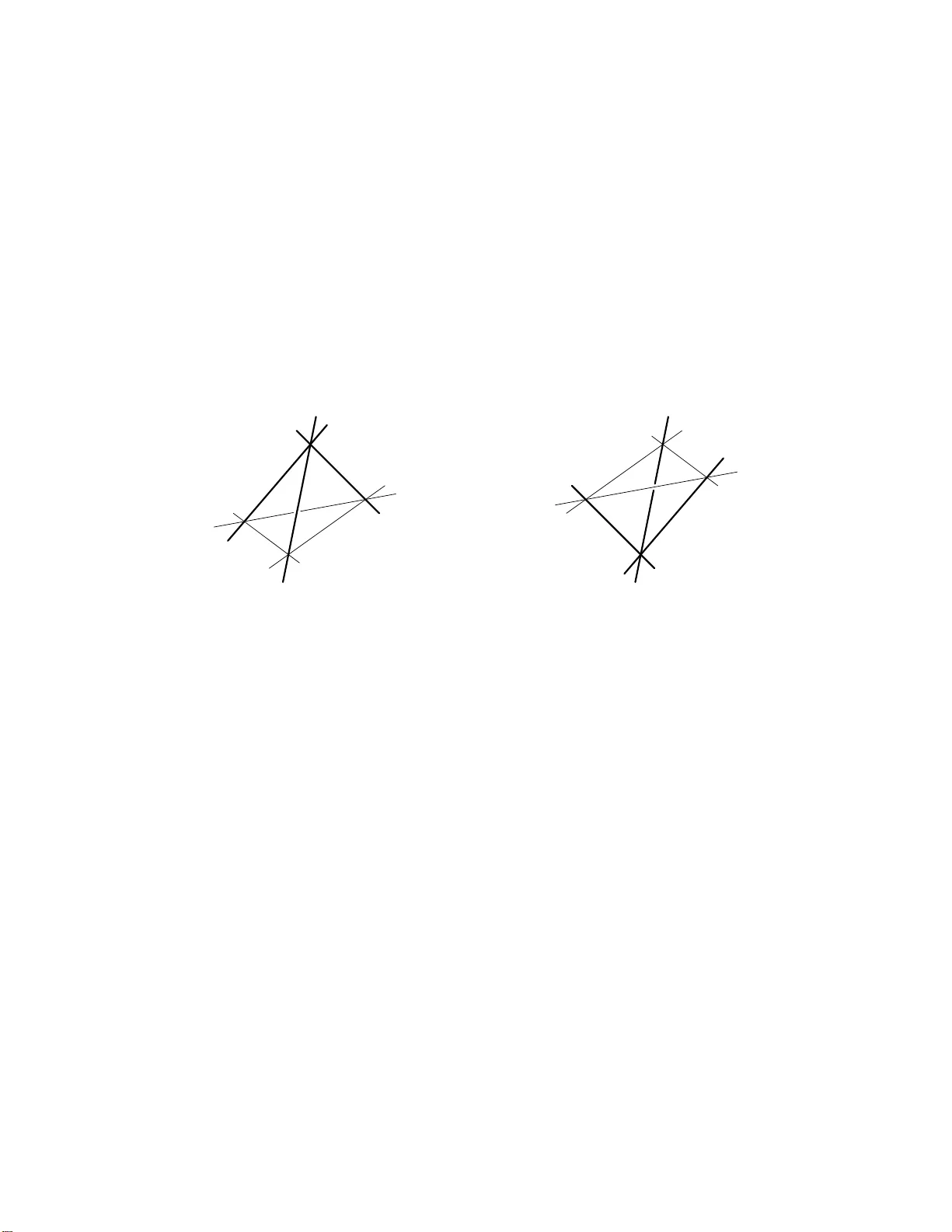
SUPER-TETRAHEDRA AND SUPER-ALGEBRAS SERGEY M. S ERGEEV Abstra ct. In this pap er w e giv e a detailed classification scheme for three-dimensional quan- tum zero curv ature represe ntatio n and tetrahedron equ ations. This sc heme includes b oth even and odd parity components, the resulting algebras of observ ables are either Bos e q - oscillators or F ermi oscillators . Three-dimensional R -matrices intert wining v ariously ori- ented tensor products of Bose and F ermi oscil lators and s atisfying tetrahedron and sup er- tetrahedron eq uations are deriv ed. The 3 d → 2 d compactification rep roduces U q ( b gl( n | m )) sup er-algebras and their representatio n theory . Introduction The q -oscilla tor solution of the quan tum tetrahedron e quation w as deriv ed in [1] as an in- terwiner of quan tum lo cal Y a n g-Baxte r equation with a sp ecific Ansatz for auxiliary m atrices. Ho we v er, a more fund amen tal zero curv ature repr esen tation of three-dimensional mo dels is based on an auxiliary linear problem [2]. Namely , the q -oscillator mo del can b e view ed as the qu an tization [3, 4] of discrete three-w av e equations and their linear p r oblem [5, 6]. In the fir st section of this pap er we discu s s in details this t yp e’s zero curv ature repr esen tation and the tetrahedron equation from the quan tu m mec hanical p oin t of view, and form ulate a classification p roblem for alg ebras of observ ables. The q -oscillato r algebra is the solution of the classification problem for ev en algebras, Theorem 1 of the second section. T he linear problem pro vides a natural wa y to in tro du ce also o dd algebras and extend the classification problem to mixed case of ev en and o dd algebras, corresp onding classificatio n T heorem 2 is the sub ject of the second section as w ell. The result of classifica tion theorem is the existence of four distinct automorphisms for ev en algebras A ( q ± 1 ) and od d alg ebras F ( q ± 1 ) and eigh t (sup er-)tetrahedra for them. Bose and F ermi oscillators are “ev aluation represen tations” of f ormal algebras A ( q ± 1 ) and F ( q ± 1 ). Th ese represen tations are fixed in the third section. In the four th section w e c onstruct explicitly all corresp onding qu an tum int ert winer s ( R -matrices) and in the fifth section we discuss br iefly all eig ht tet r ahedron equ ations. 1991 Mathematics Subje ct Classific ation. 37K15. Key wor ds and phr ases. T etrahedron Equ ations, 3-wa ve equations, Y ang-Baxter equation, Sup er-algebras. 1 2 S. SER GEEV An y sol ution of the tetrahedron equation pro du ces a series of solutions of the Y a n g-Baxte r equation. In section six we remind this sc heme for the obtained Bose/F ermi inhomoge- neous solutions of the tetrahedron equ ations. The resulting quan tum groups are i n ge n- eral U q ( b gl( n | m )). T his statement is detailed in th e last section for the illustrativ e case of U q ( b gl(2 | 1)) 1. Zero cur v a ture repre sent a ti on. The primary concept of in tegrabilit y is an auxiliary linear problem. Th e simplest form of lo cal au x iliary linear problem in th e theory of quan tum integ rable systems in w h olly discrete 2 + 1 dimensional s pace-time is the pair of linear relati ons [7] (1) ψ ′ α = a j ψ α + b j ψ β , ψ ′ β = c j ψ α + d j ψ β , where a j , b j , c j , d j are elements of some lo cal algebra C j , (2) C j = C [ a j , b j , c j , d j ] , and ψ α , ψ ′ α , ψ β , ψ ′ β are auxiliary linear elements f rom a formal left mo d ule of a tens or pow er of lo cal alge b ras. Geometrical ly , a collection of lo cal linear p roblems is associated w ith a 2 d “space-lik e” section of a three-dimensional graph, see Fig. 1. Auxiliary v ariables are asso ciated with the edges of auxiliary plane, wh ile the elements of C j are asso ciated with the j th v ertex of auxiliary plane which corresp onds to a “time-lik e” edge of the 3 d graph (b old edge in Fig. 1). It is con v enien t to rewrite the lo cal linear p roblem in a m atrix form, ψ α ψ ′ α ψ β ψ ′ β C j Figure 1. 3 d geometry of auxiliary linear problem. (3) ψ ′ α ψ ′ β ! = X αβ [ C j ] ψ α ψ β ! , X αβ [ C j ] = a j b j c j d j ! , where X αβ [ C ] is a tru e 3 d analogue of a L ax op erator. C ollect ion of lo cal linear problems along an auxiliary 2 d graph relates the outer auxiliary v ariables. F or the triangle graph in SUPER-TETRAHEDRA AND SUPER-ALGEBRAS 3 Fig. 2 the lo cal linear problems allo w one to express ψ ′′ α , ψ ′′ β and ψ ′′ γ as linear com binations of ψ α , ψ β and ψ γ . These expressions can b e written in the matrix form as (4)    ψ ′′ α ψ ′′ β ψ ′′ γ    = X αβ [ C 1 ] X αγ [ C 2 ] X β γ [ C 3 ] ·    ψ α ψ β ψ γ    , where X αβ is the tw o-b y-t wo matrix (3) in the blo c k α ⊕ β completed by the unit y in the blo c k γ , etc. ψ β ψ ′′ β ψ γ ψ ′′ γ ψ α ψ ′′ α C 2 C 3 C 1 Figure 2. Aux iliary linear prob lem for a triangle . One can consider an “opp osite” graph to Fig. 2 , shown in Fig. 3. The opp osite graph has the same external data a s the initial o ne: the co llection of linear pr ob lems also allo w s to exp eress ψ ′′ α , ψ ′′ β and ψ ′′ γ as lin ear com binations of ψ α , ψ β and ψ γ : (5)    ψ ′′ α ψ ′′ β ψ ′′ γ    = X β γ [ C ′ 3 ] X αγ [ C ′ 2 ] X αβ [ C ′ 1 ] ·    ψ α ψ β ψ γ    , with some C ′ j = C [ a ′ j , b ′ j , c ′ j , d ′ j ]. ψ β ψ ′′ β ψ γ ψ ′′ γ ψ α ψ ′′ α C ′ 2 C ′ 1 C ′ 3 Figure 3. Op p osite triangle. Zero curv ature condition is the complete indep en dence of linear problem of a choic e of graphs, Fig. 2 and Fig. 3: (6) X αβ [ C 1 ] X αγ [ C 2 ] X β γ [ C 3 ] = X β γ [ C ′ 3 ] X αγ [ C ′ 2 ] X αβ [ C ′ 1 ] . This equation resem b les the lo cal Y ang-Baxter equation, ho w ever (6) is the equation in tensor sum of spaces α, β and γ . Equation (6) for C -v alued fields C w as stud ied in details b y I. 4 S. SER GEEV Korepano v in [7], some earlier applications of (6) to functional tetrahedron equation can b e found in [8]. In classics, when C j are Ab elian algebras, equation (6) is just an equation of motion f or C - v alued fields a j , b j , c j , d j since the zero curv ature condition is just a self-consistency condition for the linear problems. In the co nv enti onal classical approac h the gauge symm etry of auxiliary fields, ψ α → G α ψ α , e tc., is u sed to reduce the n umb er of indep endent fi elds : (7) a j = 1 , b j = − A j , c j = A ∗ j , d j = 1 − A j A ∗ j , what corresp onds to auxilia ry relations ψ α − ψ ′ α = A j ψ β and ψ ′ β − ψ β = A ∗ j ψ ′ α of the discrete three-w av e system [6]. Our aim, ho we ver, is a quan tum theory where the gauge transformations affec tin g quan- tum structur e m ust b e considered more carefully . Y et the algebras C j and C ′ j are un certain. What w e exp ect from the foun dations of quantum theories: quantum equations of motion are conjugations by a discrete time ev olution op er ator and therefore the Heisen b erg quantum equations of motion in discrete sp ace-t ime are sequences of automorph isms. F ollo wing the foun dations of quan tum theories, supp ose no w that algebras C 1 , C 2 and C 3 are lo cal and equiv alen t: the triplet [ C 1 , C 2 , C 3 ] is the tensor pro duct of three indep endent copies of the same algebra, (8) [ C 1 , C 2 , C 3 ] = C 1 ⊗ C 2 ⊗ C 3 = C ⊗ 3 so that the index j sta nds for the comp onent of t ensor pro duct 1 . Then one co m es to a Problem: What is an algebr a C such that e quation (6) defines uniquely an automorphism C ⊗ 3 → C ⊗ 3 , (9) C 1 ⊗ C 2 ⊗ C 3 → C ′ 1 ⊗ C ′ 2 ⊗ C ′ 3 . Natural extension of this problem is the case of n on -equiv alen t algebras C j . W e will prov e the classification th eorems for this problem in the next sect ion. Our fi n al aim is the explicit co nstruction of in tertwining op erators for quan tum equation (6). If algebras C j and th eir irreducible representa tions are c hosen prop erly , then the automorph ism (9) is in ternal one: there exists an uniquely defined o p erator R 123 suc h that (10) C ′ j = R 123 C j R − 1 123 , j = 1 , 2 , 3 . 1 formally , C j now stands for an env eloping algebra of [1 , a j , a − 1 j , b j , c j , d j , d − 1 j ]. SUPER-TETRAHEDRA AND SUPER-ALGEBRAS 5 Indices of R 123 refer to the comp onents of tensor pro d uct V 1 ⊗ V 2 ⊗ V 3 of represen tation spaces of C 1 ⊗ C 1 ⊗ C 3 . Equation (6) ta k es the form (11) X αβ [ C 1 ] X αγ [ C 2 ] X β γ [ C 3 ] R 123 = R 123 X β γ [ C 3 ] X αγ [ C 2 ] X αβ [ C 1 ] , see Fig. 4 for the graphical representat ion of this in tertwining relation. Equ ation (11) can b e view ed as one of p ossib le 3 d extensions of Quantum group’s intert wining of co-pro ducts R ∆ = ∆ ′ R . γ α β 2 3 1 γ α β 2 3 1 = Figure 4 . Graphical represen tation of E quation (11): auxiliary t r iangles f rom Figs. 2 and 3 with the sol id v ertex standing for the intert wini ng oper ator R 123 . Auxiliary planes are sections of the solid vertex of t hree-dimensional lattice. Equat i on (11) has the struct ure of tetrahedron eq uation in V 1 ⊗ V 2 ⊗ V 3 ⊗ ( α ⊕ β ⊕ γ ). Op erators R ij k satisfy a n associativit y condition follo wing from equiv alence (12) X αβ [ C 1 ] X αγ [ C 2 ] X β γ [ C 3 ] X αδ [ C 4 ] X β δ [ C 5 ] X γ β [ C 6 ] = X γ β [ C ′′ 6 ] X β δ [ C ′′ 5 ] X αδ [ C ′′ 4 ] X β γ [ C ′′ 3 ] X αγ [ C ′′ 2 ] X αβ [ C ′′ 1 ] This automorphism of sixth tensor p o we r can b e decomp osed in to elemen tary automorph isms in tw o d ifferen t w a y s : (13) T L = R 123 R 145 R 246 R 356 and T R = R 356 R 246 R 145 R 123 . Due to the uniqu eness of auto morphisms, b oth wa ys coincide: (14) T L = T R , what is the te trahedron equation – the three-dimensional generalization of the Y ang-Baxter (triangle) equ ation. Graphical represen tation of the te tr ahedron equatio n is g iv en in Fig . 5 6 S. SER GEEV V 1 V 5 V 3 V 4 V 2 V 6 V 1 V 5 V 3 V 4 V 2 V 6 = Figure 5. Graphical represen tation of th e tetrahedron equ ation (14) in V 1 ⊗ · · · ⊗ V 6 : equiv al ence of t wo three-dimensional graphs. 2. Classifica tion theorems 2.1. Ev en case. The answe r to the p roblem ab o v e is Theorem 1. Equation (6) defines an automorphism of tenso r cub e of C is and only if (15) C [ a, b, c, d ] = A ( q ; a, b, c, d ) wher e A ( q ) is define d by (16) ad = da , ab = q ba , ca = q ac , db = q bd , cd = q dc , bc − cb = ( q − 1 − q ) ad . Algebra A ( q ) has t w o cen ters, (17) η = ad − 1 and ξ = q − 1 ad − bc . The inv erse relatio n for A ( q ) is (18) a b c d ! − 1 = 1 ξ q − 1 d − b − c q a ! . W e consider the cen ters η j and ξ j of A j ( q ) as C -numerical parameters of A j ( q ). Under this assumption A ( q ) b ecomes the q -oscilla tor algebra fr om [1]. Sk etch pro of. Whic hev er C j are taken, • the non-primed elements of C j with differen t j commute sin ce j stands for a comp onent of t ensor p ro duct, C 1 = C ⊗ 1 ⊗ 1 , e tc. • w e are lo oking for an au tomorp h ism. This means in p articular, pr imed elemen ts of C ′ j with d ifferen t j al so m ust co mm u te. SUPER-TETRAHEDRA AND SUPER-ALGEBRAS 7 This is called (ultra-)lo calit y , the starting p oin t o f the pro of is its test. Matrix equatio n (6) in comp onen ts reads: (19) a ′ 2 a ′ 1 = a 1 a 2 , d ′ 3 d ′ 2 = d 2 d 3 , (20) a ′ 2 b ′ 1 = b 1 a 3 + a 1 b 2 c 3 , c 1 a 2 = a ′ 3 c ′ 1 + b ′ 3 c ′ 2 a ′ 1 , b ′ 2 = b 1 b 3 + a 1 b 2 d 3 , c 2 = c ′ 3 c ′ 1 + d ′ 3 c ′ 2 a ′ 1 , b ′ 3 d ′ 2 = d 1 b 3 + c 1 b 2 d 3 , d 2 c 3 = c ′ 3 d ′ 1 + d ′ 3 c ′ 2 b ′ 1 and finally , (21) a ′ 3 d ′ 1 + b ′ 3 c ′ 2 b ′ 1 = d 1 a 3 + c 1 b 2 c 3 . Note, th e left column in (20) gives almost explicit expr essions for prim ed b j . The lo calit y of C ′ 1 and C ′ 2 implies in particular (22) [ b ′ 2 , a ′− 1 1 b ′ 1 ] ≡ [ b 1 b 3 + a 1 b 2 d 3 , ( a 1 a 2 ) − 1 ( b 1 a 3 + a 1 b 2 c 3 )] = 0 Expanding the comm utator, w e ha ve (23) ( b 1 a − 1 1 b 3 a 3 − a − 1 1 b 1 a 3 b 3 ) b 1 a − 1 2 +( b 2 a − 1 2 d 3 c 3 − a − 1 2 b 2 c 3 d 3 ) a 1 b 2 + b 1 b 2 a − 1 2 d 3 a 3 − a − 1 1 b 1 a 1 a − 1 2 b 2 a 3 d 3 + b 1 a − 1 2 b 2 [ b 3 , c 3 ] = 0 Here the lo calit y of C j is tak en in to accoun t. Chec k no w the s tr ucture of three lines here in C 2 . The first lin e has a − 1 2 , the second line has a − 1 2 b 2 2 , t he third lin e has a − 1 2 b 2 . Since one ca n hardly exp ect ab ∼ ba ∼ a , we can conclude that the whole expression is zero if eac h line is zero. Th e first line giv es (24) b 1 a − 1 1 b 3 a 3 = a − 1 1 b 1 a 3 b 3 ⇒ ab = q ba for some q . Th e second lin e giv es (25) b 2 a − 1 2 d 3 c 3 = a − 1 2 b 2 c 3 d 3 ⇒ cd = q dc with the same q . Finally , the third line giv es (26) [ b, c ] = q − 1 ad − q da . In a similar wa y one ca n c hec k (27) [ b ′ 2 , d ′− 1 3 b ′ 3 ] = 0 and get (28) db = q ′ bd , ca = q ′ ac , [ b, c ] = q ′− 1 da − q ′ ad 8 S. SER GEEV for some q ′ . Comparin g t wo v ariant s of [ b, c ], w e h a v e (29) q da = q ′ ad . All th e other lo calit y tests provi de no additional information. Th u s, the lo calit y test giv es u s the most general form of C : (30) C ( q , q ′ ) :      ab = q ba , cd = q dc , db = q ′ bd , ca = q ′ ac , [ b, c ] = ( q − 1 − q ′ ) ad , qda = q ′ ad One can ve rify fur th er, for C j = C ( q , q ′ ) the system of relations (6) is self-consisten t: not only lo calit y but relations (30) for p rimed elemen ts do n ot con tradict the system (6). How ev er, w e ha ve no uniqueness y et. Nine equations (6) for t wel v e elemen ts do not pro duce a uniqu e map in general. The map is u nique only if C ( q , q ′ ) has cen ters and the map conserv es them (cen ters of algebras comm ute with their in tert winer, Eq. (10)) . It is easy to ve rify the follo win g Lemma: The algebr a C ( q , q ′ ) has c enters c omp atible with (6) if and only if q = q ′ . This lemma can b e pr o v en in quasiclassical limit q = e ℏ → 1 and q ′ = e ℏ ′ → 1, so that ℏ / ℏ ′ = δ as a parameter of P oisson algebra. Equation for a cen ter of Poisson algebra is a system of differen tial equation w ith trivial solution u nless δ 6 = ± 1. Conserv ation of cen ters for the case δ = − 1, what is q ′ = q − 1 and [ b, c ] = 0, cont r adict with (6). Th us q = q ′ is the only c h oice. Final step: when the cen ters (17) conserve, (31) cen ters of A j = cente rs of A ′ j for all j , w e can s olve (19,20,21) with resp ect to all p rimed generators (equation (18) is of exceptional use) and v erify directly that this is the automorphism of A ( q ) ⊗ 3 .  Remark: in this pro of we initially considered C ⊗ 3 framew ork – the tensor cub e of the same algebra. Ho wev er, the answer is the same without th is assump tion; th e equiv alence of C j follo ws from analysis of all p ossible lo calit y relations. Another remark concerns the case q ′ 6 = q . In general, C ( q , q ′ ) = Qsc q q ′ ⊗ W eyl q /q ′ , the W eyl subalgebra is generated by η and ξ , η · ξ =  q q ′  2 ξ · η . F or instance, th e algebras C ( q 2 , 1) and C (1 , q 2 ) app ear in the three-dimensional approac h to sp ectral equations [9]. Du e to am b iguit y , equation (11) do es not define in tertwiner R for C ( q , q ′ ) ⊗ 3 uniquely . Ho we ver, su c h in tert winer satisfying the tetrahedron equation can b e constructed b y dr essing the constant q -oscillator R -matrix (Eq. (64) b elo w) b y n on-comm utativ e exp onential factors. 2.2. Odd case. Theorem 1 is based on the lo calit y pr inciple: elemen ts in differen t comp o- nen ts of a tensor pro du ct co mm u te. This is th e feature of ev en alge bras; for o dd algebras their o dd ele men ts in differen t components of a tensor p ro duct an ti-commute. SUPER-TETRAHEDRA AND SUPER-ALGEBRAS 9 A natural (and only possib le) wa y to in tro du ce o dd algebras is to assign a parit y to auxiliary v ariables, for instance to mo dify the linear problem as foll o ws: (32) ψ ′ α = a j ψ α + b j ψ β , ψ ′ β = c j ψ α + d j ψ β . Here the un der-line symb ol mark s the o dd parit y , relations (32) corresp ond to the c h ange of parit y of aux iliary β -line. T h u s , the o dd algebras corresp ond to parit y c hanges of some of the lines α , β or γ in equatio n (6); in general there are eight differen t parit y patterns of α, β , γ . This wa y is the only p ossible one since it tak es into a ccoun t the parit y conserv ation in equation (6). Now we are ready to extend Theorem 1: Theorem 2. Given X αβ = X αβ [ A ( q )] , e quations (6) pr ovide automo rphisms if and only if (33) X αβ = X αβ [ F ( q )] , X αβ = X αβ [ F ( q − 1 )] , X αβ = X αβ [ A ( q − 1 )] for al l p arity p atterns, wher e F ( q ) = F ( q ; a, b , c, d ) (o dd elements ar e underline d) is define d by (34) ad = da , ab = q ba , ca = q ac , bd = q db , dc = q cd , bc + cb = ( q − q − 1 ) ad . F or the o dd el emen ts of F ( q ± 1 ) we ha ve (35) b 2 = c 2 = 0 . Algebra F ( q ) h as t wo centers ξ and η as w ell, (36) ξ = ad , and η is defined b y (37) q ad − b c = η d 2 , q ad − cb = η − 1 a 2 . The inv ersion relatio n for F ( q ) is (38) a b c d ! − 1 = q ξ η − 1 a − b − c η d ! . W e consider the cente rs η j and ξ j of F j ( q ) as C -numerical parameters of F j ( q ). Note also the existence o f tw o orthogo nal pro jectors in F ( q ): (39) P 1 = q a − η d , P 2 = q d − η − 1 a , suc h that (40) P 1 P 2 = b P 1 = P 1 c = cP 2 = P 2 b = 0 . 10 S. SER GEEV Sk etch pro of of Theorem 2. Consider as an examp le the parity pattern αβ γ . B y the condition of the theorem, C 2 = A 2 ( q ) while C 1 and C 3 are uncertain, bu t c 1 , 3 and b 1 , 3 are o dd elemen ts. The lo calit y test: whic h ev er C 1 and C 3 are taken, the ultra-localit y demands (41) ( a 2 b 1 b 2 − q b 2 a 2 b 1 ) ′ = ( b 3 d 2 b 2 − q b 2 b 3 d 2 ) ′ = ( a 2 b 1 b 3 d 2 + b 3 d 2 a 2 b 1 ) ′ = 0 . Here we tak e into accoun t C ′ 2 = A ′ 2 ( q ) and the parit y of C ′ 1 and C ′ 3 . Im m ediate consequence of (41) is (42) a 1 b 1 = q b 1 a 1 , c 1 a 1 = q a 1 c 1 , c 1 b 1 + b 1 c 1 = ( q − q − 1 ) a 1 d 1 and (43) c 3 d 3 = q d 3 c 3 , d 3 b 3 = q b 3 d 3 , c 3 b 3 + b 3 c 3 = ( q − 1 − q ) a 3 d 3 . Therefore, C 1 = F 1 ( q − 1 ) an d C 3 = F 3 ( q ) according to the definition (34). The fi nal step of the pro of: when th e cen ters (36) and (37) conserve, (44) cen ters of C j = cente rs of C ′ j for all j then equations (6) can be solv ed with resp ect to all pr imed ele m en ts (again with an inte n- siv e use of in version relatio n (38)) and one can v erify directly that (6) pro vid e an unique automorphism of (45) F 1 ( q ) | {z } αβ ⊗ A 2 ( q ) | {z } αγ ⊗ F 3 ( q − 1 ) | {z } β γ . All the other parity patterns ca n b e co nsidered similarly .  3. “Ev alua tion represent a tions” of A ( q ± 1 ) and F ( q ± 1 ) Before the deriv ation of in tertwining op erators we must choose firstly irredu cible rep r esen- tations of A ( q ± 1 ) and F ( q ± 1 ). Alg ebra A is equiv alent t o Bose q -oscillat or extended by tw o C -v alued parameters (cen ters of A ( q )). Algebra F is equiv alen t to F ermi oscillator with t w o extra C -v alued paramete rs. In all considerations b elo w w e imply 0 < | q | < 1. 3.1. Bose q - oscillator. W e define the Bose oscillator b y (46) a + a − = 1 − q 2 N , a − a + = 1 − q 2 N +2 , [ N , a ± ] = ± a ± . F or shortness we u se (47) q N = k . SUPER-TETRAHEDRA AND SUPER-ALGEBRAS 11 The F o c k space repr esen tations are defined either by (48) a − | 0 i = 0 , Sectrum( N ) = 0 , 1 , 2 , 3 , . . . where | 0 i is the F ock v acuum, or by (49) a + | − 1 i = 0 , Sectrum( N ) = − 1 , − 2 , − 3 , − 4 , . . . where | − 1 i i s an “anti -v acuum”. These t w o r ep resen tations are rela ted b y t h e external automorphism ι , (50) ι ( k ) = q − 1 k − 1 , ι ( a + ) = a − k − 1 , ι ( a − ) = − k − 1 a + . Here we prefer not to fix scales of a ± and u se a ± → ξ ± 1 a ± in v ariant formalism. 3.2. F ermi osc illa t or. F ermi osc illator is defined b y (51) [ f + , f − ] + = (1 − q 2 ) , [ M , f ± ] = ± f ± , ( f + ) 2 = ( f − ) 2 = 0 , where [ , ] + stands f or ant i-commutat or. Fields f ± ha ve o dd p arit y . F or instance, th e lo calit y of t w o copies F 1 and F 2 of F ermi oscillators means (52) f 1 f 2 + f 2 f 1 = 0 , etc. The F o c k v acuu m is ann ih ilated by f − . Since S p ectrum( M ) = 0 and 1, th e F o ck sp ace represent ation of F ermi oscil lator implies in addition g ( M ) = g (0)(1 − M ) + g (1) M , (53) M 2 = M , M f − = f + M = 0 , f − M = f − , M f + = f + , and (54) f + f − = (1 − q 2 ) M , f − f + = (1 − q 2 )(1 − M ) . Let f or the shortness aga in (55) k = q M = 1 − (1 − q ) M . Automorphism (50) f or F ermi oscillato r , ι ( M ) = 1 − M and ι ( f ± ) = f ∓ , is the in ternal one and therefore there is no necessit y to consid er it separately . 3.3. Represen tation of A ( q ) . W e choose the follo win g form of matrix X [ A ( q )]: (56) X [ A ( q )] =    λ k a + λµ a − − q µ k    , X [ A ( q )] − 1 =    k /λ a + /λµ a − − q k /µ    , where q -oscillat or is either in (48) or in (49) represent ation. In this parameterization η = − λ q µ and ξ = − λµ . 12 S. SER GEEV 3.4. Represen tation of A ( q − 1 ) . W e c ho ose (57) X [ A ( q − 1 )] =    q λ k a − λµ a + − µ k    , X [ A ( q − 1 )] − 1 =    q k /λ a − /λµ a + − k /µ    . 3.5. Represen tation of F ( q ) . W e c ho ose (58) X [ F ( q )] =    λ k f + λµ f − − q µ k − 1    , X [ F ( q )] − 1 =    k /λ f + /λµ f − − q k − 1 /µ    . In this parameterizatio n η = − λ µ and ξ = − q λµ . 3.6. Represen tation of F ( q − 1 ) . W e c ho ose (59) X [ F ( q − 1 )] =    q − 1 λ k q − 1 f − − q − 1 λµ f + − µ k − 1    , X [ F ( q − 1 )] − 1 =    q − 1 k /λ − q − 1 f − /λµ − q − 1 f + − k − 1 /µ    . 3.7. Remarks. Linear equation (3) for matrix X [ A ( q )] (56) ma y b e rewritten iden tically as (60) ψ ′ β ψ α ! = e X β α ψ β ψ ′ α ! , e X β α = − µq − 1 k − 1 µ a − k − 1 − λ − 1 k − 1 a + λ − 1 k − 1 ! , so that e X β α ∼ ι ( X αβ ) up to a c h ange of sp ectral parameters. Th u s, a c hange of orien tation of linear problem (see Fig. 1) is equiv alent to ι -automorphisms (50 ). 4. Eight inter twining rel a tions In this section w e giv e the list of in tertwining op erators (11 ) for all p arit y p atterns of α, β , γ for represen tations of A ( q ± 1 ), F ( q ± 1 ) c hosen ab o ve. F or shortness, the sym b ols A and F as the indices of three-dimensional R -matrices w ill stand for corresp onding represen tation F o c k spaces. The f ollo wing eigh t in tert wining relatio n s hold. 4.1. Configuration αβ γ . The b asic inte rt win ing r elatio n is (61) X αβ [ A 1 ( q )] X αγ [ A 2 ( q )] X β γ [ A 3 ( q )] R = R X β γ [ A 3 ( q )] X αγ [ A 2 ( q )] X αβ [ A 1 ( q )] . The intert winer here is (62) R = R A 1 ( q ) A 2 ( q ) A 3 ( q ) ( u, v , w ) = v N 2 R A 1 A 2 A 3 u N 1 w N 3 , SUPER-TETRAHEDRA AND SUPER-ALGEBRAS 13 where f or brevity (63) u = λ 3 λ 2 , v = λ 1 µ 3 , w = µ 1 µ 2 . This d efi nition of parameters u, v , w is used in all cases b elo w . Cons tant matrix R can b e written as a p o w er series (64) R A 1 A 2 A 3 = R 0 ( N 1 , N 2 , N 3 ) + ∞ X k =1  R k ( N 1 , N 2 , N 3 )( a − 1 a + 2 a − 3 ) k + ( a + 1 a − 2 a + 3 ) k R k ( N 1 , N 2 , N 3 )  , where the co efficient s R k ( N 1 , N 2 , N 3 ) are giv en by expansion of three equiv alen t generating functions: (65) T r A 1  z N 1 a − k 1 a + k 1 R k ( N 1 , N 2 , N 3 )  = z N 2 − k ( q N 3 − N 2 + k +2 z − 1 ; q 2 ) ∞ ( q N 3 + N 2 − k +2 z − 1 ; q 2 ) ∞ ( q N 3 + N 2 + k +2 z ; q 2 ) ∞ ( q N 3 − N 2 + k z ; q 2 ) ∞ , (66) T r A 2  z N 2 a − k 2 R k ( N 1 , N 2 , N 3 ) a + k 2  = q N 1 N 3 ( − q 1 − N 1 − N 3 z ; q 2 ) ∞ ( − q 3+ N 1 + N 3 +2 k z ; q 2 ) ∞ ( − q 1 − N 1 + N 3 z ; q 2 ) ∞ ( − q 1+ N 1 − N 3 z ; q 2 ) ∞ , and (67) T r A 3  z N 3 a − k 3 a + k 3 R k ( N 1 , N 2 , N 3 )  = z N 2 − k ( q N 1 − N 2 + k +2 z − 1 ; q 2 ) ∞ ( q N 1 + N 2 − k +2 z − 1 ; q 2 ) ∞ ( q N 1 + N 2 + k +2 z ; q 2 ) ∞ ( q N 1 − N 2 + k z ; q 2 ) ∞ . Here we use the standard q -hyp ergeometric notations [10]: (68) ( x ; q 2 ) n = n − 1 Y k =0 (1 − xq 2 k ) , ( x ; q 2 ) ∞ = ∞ Y k =0 (1 − xq 2 k ) . These generating functions are v alid for b oth repr esen tations (4 8 ) an d (49) for an y of A 1 , A 2 , A 3 . Note, for fin ite in teger N j and k all generating f unctions are rational functions regular at z = 0 and at z = ∞ with finite n umb er of p oles in z -plane, a generation function F ( z ) = T r A z N f ( N ) gives f ( N ) as expansion near z = 0 or near z = ∞ for representa tions (48) or (49) resp ectiv ely . Th e exp ressions for R k ( N 1 , N 2 , N 3 ) in terms of q -hyper geometric function can b e obtained b y Cauch y integral s of generating f u nctions, in particular the matrix element s of (64) for representat ion (48) in all A 1 , A 2 , A 3 are given in [1, 4]. Note a few symm etry p rop erties. Firstly , generating functions pr o vide the defin ition of R k for n egativ e k , (69) R − k ( n 1 + k , n 2 − k , n 3 + k ) = ( q 2 ; q 2 ) n 1 + k ( q 2 ; q 2 ) n 2 ( q 2 ; q 2 ) n 3 + k ( q 2 ; q 2 ) n 1 ( q 2 ; q 2 ) n 2 − k ( q 2 ; q 2 ) n 3 R k ( n 1 , n 2 , n 3 ) . P ow er series (64) ca n b e form ally rewritten as (70) R A 1 A 2 A 3 = ∞ X k = −∞ R k ( N 1 , N 2 , N 3 )( a − 1 a + 2 a − 3 ) k = ∞ X k = −∞ ( a + 1 a − 2 a + 3 ) k R k ( N 1 , N 2 , N 3 ) , 14 S. SER GEEV where R k ≡ 0 at states where negativ e p ow ers of creatio n and annihilation op erators are not defined. Op erator (64) is th e square root of unit y , (71) R − 1 A 1 A 2 A 3 = R A 1 A 2 A 3 for any choice of rep r esen tations (48,49). Remark ably , an analytic p ro of of this statemen t in volv es the Raman ujan summation formula [10]. Also, expression (64) has the eviden t s y m - metry with resp ect to an an ti-inv olution N → N and a ± → a ∓ . Th is anti-in v olution is the Hermitian conju gatio n for real q and un itary representa tion (48). Op erator (64) is th e unique solution of ( 61) pro vided the in teger sp ectra of N j . 4.2. Configuration αβ γ . Relation (72) X αβ [ A 1 ( q − 1 )] X αγ [ A 2 ( q − 1 )] X β γ [ A 3 ( q − 1 )] R = R X β γ [ A 3 ( q − 1 )] X αγ [ A 2 ( q − 1 )] X αβ [ A 1 ( q − 1 )] pro vid es (73) R = R A 1 ( q − 1 ) A 2 ( q − 1 ) A 3 ( q − 1 ) ( u, v , w ) = v − N 2 R A 1 A 2 A 3 u − N 1 w − N 3 . where u, v , w and R A 1 A 2 A 3 are giv en by (63) an d (64). 4.3. F ermionic configurations a nd intert winers. In tert wining op erators for the fermions can b e p resen ted in t wo wa ys . One is the w ay of m atrix elemen ts for the basis of f ermionic states, eve n v acuum | 0 i and o dd one-fermion state | 1 i = f + √ 1 − q 2 | 0 i ; all equations in matrix elemen ts will ha ve then unpleasan t sign factors taking into accoun t the o dd parity of the state | 1 i and ordering of fermions. Another wa y a v oiding the sign factors is to consider fermionic op erators directly as expressions in terms of o dd f er m ionic creatio n and ann ihilation op erators lik e in [1 1 ]. W e c ho ose the sec ond w a y here. Besides, the expressions fo r the fermionic in tertwiners b elo w do not need inte ger s p ectra of Bose oscillators and therefore they are v alid also for the mo du lar r epresen tation of q -oscillator [4]. 4.4. Configuration α β γ . Relation (74) X α β [ F 1 ( q − 1 )] X α γ [ F 2 ( q − 1 )] X β γ [ A 3 ( q )] R = R X β γ [ A 3 ( q )] X αγ [ F 2 ( q − 1 )] X α β [ F 1 ( q − 1 )] yields un iquely (75) R = R F 1 ( q − 1 ) F 2 ( q − 1 ) A 3 ( q ) ( u, v , w ) = v − M 2 R F 1 F 2 A 3 u − M 1 w N 3 where th e constan t matrix R is (76) R F 1 F 2 A 3 = (1 − M 1 )(1 − M 2 ) + q M 1 (1 − M 2 ) k 3 − (1 − M 1 ) M 2 k 3 − M 1 M 2 + f + 1 f − 2 a − 3 − f − 1 f + 2 a + 3 1 − q 2 SUPER-TETRAHEDRA AND SUPER-ALGEBRAS 15 and u, v , w are giv en by (63). C onstan t R -matrix is the ro ot o f unit y , (77) R F 1 F 2 A 3 = R − 1 F 1 F 2 A 3 , and expression (76) is symmetric with resp ect to f ± → f ∓ , a ± → a ∓ an ti-inv olution. 4.5. Configuration αβ γ . Relation (78) X αβ [ F 1 ( q )] X αγ [ F 2 ( q )] X β γ [ A 3 ( q − 1 )] R = R X β γ [ A 3 ( q − 1 )] X αγ [ F 2 ( q )] X αβ [ F 1 ( q )] yields (79) R = R F 1 ( q ) F 2 ( q ) A 3 ( q − 1 ) ( u, v , w ) = v M 2 R F 1 F 2 A 3 u M 1 w − N 3 where th e constan t matrix R F 1 F 2 A 3 is giv en b y (76). 4.6. Configuration αβ γ . Relation (80) X αβ [ A 1 ( q )] X αγ [ F 2 ( q )] X β γ [ F 3 ( q )] R = R X β γ [ F 3 ( q )] X αγ [ F 2 ( q )] X αβ [ A 1 ( q )] pro vid es uniqu ely (81) R = R A 1 ( q ) F 2 ( q ) F 3 ( q ) ( u, v , w ) = v M 2 R A 1 F 2 F 3 u N 1 w M 3 where (82) R A 1 F 2 F 3 = (1 − M 2 )(1 − M 3 ) − q k 1 M 2 (1 − M 3 ) + k 1 (1 − M 2 ) M 3 − M 2 M 3 + a − 1 f + 2 f − 3 − a + 1 f − 2 f + 3 1 − q 2 Op erator (82) is the square ro ot of unit y symmetric w ith resp ect to th e anti- in volutio n. 4.7. Configuration αβ γ . Relatio n (83) X αβ [ A 1 ( q − 1 )] X α γ [ F 2 ( q − 1 )] X β γ [ F 3 ( q − 1 )] R = R X β γ [ F 3 ( q − 1 )] X αγ [ F 2 ( q − 1 )] X αβ [ A 1 ( q − 1 )] giv es (84) R = R A 1 ( q − 1 ) F 2 ( q − 1 ) F 3 ( q − 1 ) ( u, v , w ) = v − M 2 R A 1 F 2 F 3 u − N 1 w − M 3 where R A 1 F 2 F 3 is giv en b y (82). 16 S. SER GEEV 4.8. Configuration αβ γ . Relatio n (85) X αβ [ F 1 ( q )] X αγ [ A 2 ( q )] X β γ [ F 3 ( q − 1 )] R = R X β γ [ F 3 ( q − 1 )] X αγ [ A 2 ( q )] X αβ [ F 1 ( q )] giv es uniquely (86) R = R F 1 ( q ) A 2 ( q ) F 3 ( q − 1 ) = v N 2 R F 1 A 2 F 3 u M 1 w − M 3 where (87) R F 1 A 2 F 3 = ( − q ) − N 2  (1 − M 1 ) k 2 (1 − M 3 ) + q − 1 M 1 (1 − M 3 ) + (1 − M 1 ) M 3 + M 1 k 2 M 3 + q − 1 f + 1 a − 2 f − 3 − f − 1 a + 2 f + 3 1 − q 2  Op erator (87) is the ro ot of unit y but it is n ot symm etric with resp ect to the an ti-inv olution. 4.9. Configuration α β γ . Relation (88) X α β [ F 1 ( q − 1 )] X αγ [ A 2 ( q − 1 )] X β γ [ F 3 ( q )] R = R X β γ [ F 3 ( q )] X αγ [ A 2 ( q − 1 )] X αβ [ F 1 ( q − 1 )] pro duces (89) R = R F 1 ( q − 1 ) A 2 ( q − 1 ) F 3 ( q ) ( u, v , w ) = v − N 2 R F 1 A 2 F 3 u − M 1 w M 3 where R F 1 A 2 F 3 is giv en b y (87). 4.10. Remarks. All constan t R -matrices are ro ots of u nit y since for λ = µ = 1 (90) X [ C ] = X [ C ] − 1 for a ll X -matrixes (56-59). Also, m atrices X [ A ( q )], X [ A ( q − 1 )], X [ F ( q )] at λ = µ = 1 and matrix X [ F ( q − 1 )] at λ = 1 , µ = − 1 are symmetric with resp ect to the an ti-inv olution a ± → a ∓ and f ± → f ∓ accompanied b y the matrix transp osition. Recall, this an ti-in vo lution is the Hermitian co njugation for 0 < q < 1 for F ermi oscillators and Bose oscillat or in represent ation (48). Represent ation (49) of Bose oscillator admits ( a ± ) † = − a ∓ . Thus, the unitarit y of in tertwiners is an extra condition fixing a p rop er choic e of represen tations (48) or (4 9 ). F or instance, R F 1 , F 2 , A 3 and R A 1 , F 2 , F 3 are u nitary for representat ion (48) for A 1 and A 3 while R F 1 , A 2 , F 3 is unitary for r epresen tation (49) of A 2 . Matrix R A 1 , A 2 , A 3 is u nitary if represent ation (49) is c h osen in ev en n umb er of c omp onen ts A 1 , A 2 , A 3 . SUPER-TETRAHEDRA AND SUPER-ALGEBRAS 17 5. Examples of tetrahed ra W e ha ve four constant R -matrices, sp ectral parameters ent er as simp le exp onential fields: (91) R C 1 C 2 C 3 ( u, v , w ) = v N 2 R C 1 C 2 C 3 u N 1 w N 3 , where A ( q ) A ( q − 1 ) F ( q ) F ( q − 1 ) N N − N M − M The only difference b et w een C ( q ) and C ( q − 1 ) is the sign of a field exp onent. Note, an y m atrix R C 1 C 2 C 3 comm utes with N 1 + N 2 and N 2 + N 3 . Therefore, the sp ectral parameters can b e r emo v ed from any tetrahedron equation and finally we h a v e only eigh t constan t tetrahedron equ ations (92) R C 1 C 2 C 3 R C 1 C 4 C 5 R C 2 C 4 C 6 R C 3 C 5 C 6 = R C 3 C 5 C 6 R C 2 C 4 C 6 R C 1 C 4 C 5 R C 1 C 2 C 3 with V arian t C 1 C 2 C 3 C 4 C 5 C 6 1 A 1 A 2 A 3 A 4 A 5 A 6 2 A 1 A 2 A 3 F 4 F 5 F 6 3 A 1 F 2 F 3 A 4 A 5 F 6 4 F 1 A 2 F 3 A 4 F 5 A 6 5 F 1 F 2 A 3 F 4 A 5 A 6 6 A 1 F 2 F 3 F 4 F 5 A 6 7 F 1 A 2 F 3 F 4 A 5 F 6 8 F 1 F 2 A 3 A 4 F 5 F 6 5.1. T etrahedron A A AF F F . The quadrilateral configuration (93) X αβ [ A 1 ] X αγ [ A 2 ] X β γ [ A 3 ] X αδ [ F 4 ] X β δ [ F 5 ] X γ δ [ F 6 ] pro vid es the tetrahedron equation (94) R A 1 A 2 A 3 R A 1 F 4 F 5 R A 2 F 4 F 6 R A 3 F 5 F 6 = R A 3 F 5 F 6 R A 2 F 4 F 6 R A 1 F 4 F 5 R A 1 A 2 A 3 , n u m b er 2 from the table. Being wr itten in m atrix element s in fermionic spaces, | 1 i ∼ f + | 0 i , (95) R A 1 F 2 F 3 id ⊗ | j 2 i ⊗ | j 3 i = X i 1 ,i 2 | i 2 i ⊗ | i 3 i ( − ) p ( i 1 ) p ( i 2 ) L j 1 ,j 2 i 1 ,i 2 [ A 1 ] , where fermionic o ccupation num b ers i, j = 0 , 1 and the p arit y is p ( i ) = i , equation (94) is equiv alent to RLLL relation (4) from [1]. 18 S. SER GEEV 5.2. T etrahedron A F F F F A . Th e quadrilateral configuration (96) X αβ [ A 1 ] X α γ [ F 2 ] X β γ [ F 3 ] X αδ [ F 4 ] X β δ [ F 5 ] X γ δ [ A 6 ] pro vid es the constan t te tr ah ed ron equati on (97) R A 1 F 2 F 3 R A 1 F 4 F 5 R F 2 F 4 A 6 R F 3 F 5 A 6 = R F 3 F 5 A 6 R F 2 F 4 A 6 R A 1 F 4 F 5 R A 1 F 2 F 3 , n u m b er 6 f rom the table ab ov e. F ermionic lines in this equation are not planar, hence sign parit y f actors are irremov able from a m atrix form of (97). Ho wev er, the parity factors can b e absorb ed by a re-definition of A 6 , result is the “strange” LLM M relatio n (34) from [1]. 6. Y ang-Baxter equa tion and transfer ma trices 6.1. R -matrices of Y ang-Baxter equation. An R -matrix of the Y ang-Baxter equation can b e defined by (98) R C 1 , C 2 = T race C 3 y Y ℓ R C 1: ℓ C 2: ℓ , C 3 ! , where semicolon in indices separates t he orienta tion index j = 1 , 2 , 3 and the co ordinate indices, the ordered p ro duct stands for (99) y Y ℓ f ℓ = f 1 f 2 · · · f L , and the spaces of t wo-dimensional R -matrix are (100) C 1 = L ⊗ ℓ =1 C 1: ℓ , C 2 = L ⊗ ℓ =1 C 2: ℓ . The sequ ence of te trahedron equat ions (101) y Y ℓ R C 1: ℓ C 2: ℓ C 3 R C 1: ℓ C 4: ℓ C 5 R C 2: ℓ C 4: ℓ C 6 ! R C 3 C 5 C 6 = R C 3 C 5 C 6 y Y ℓ R C 2: ℓ C 4: ℓ C 6 R C 1: ℓ C 4: ℓ C 5 R C 1: ℓ C 2: ℓ C 3 ! pro vid e the Y ang-Baxt er equation for (98), (102) R C 1 C 2 R C 1 C 4 R C 2 C 4 = R C 2 C 4 R C 1 C 4 R C 1 C 2 . The “third” sp ace of three-dimensional R -matrix is c hosen as the h id den space in (98), in general it can b e “fir st” or “sec ond ” orien tation spaces as well. Lo cally , the sp ectral parameters en ter (98) a s (103) R C 1: ℓ C 2: ℓ , C 3 = v N 2: ℓ ℓ R C 1: ℓ C 2: ℓ , C 3 u N 1: ℓ ℓ w N 3 ℓ , SUPER-TETRAHEDRA AND SUPER-ALGEBRAS 19 see (91), where (104) u ℓ = λ 3 λ 2: ℓ , v ℓ = λ 1: ℓ µ 3 , w ℓ = µ 1: ℓ µ 2: ℓ . Since N 1 + N 2 and N 2 + N 3 comm ute with R C 1 C 2 C 3 , the expression for (98) can b e rewritten iden tically as (105) R C 1 C 2 = U − 1 1 U − 1 2 Y ℓ v N 2: ℓ ℓ ! R C 1 C 2 ( µ 1 /µ 2 ) Y ℓ u N 1: ℓ ℓ ! U 1 U 2 , where th e gauge fact ors are (106) U 1 = L Y ℓ =1 µ P ℓ ℓ ′ =0 N 1: ℓ ′ 1: ℓ , U 2 = L Y ℓ =1 µ P ℓ ℓ ′ =0 N 2: ℓ ′ 2: ℓ , the simplifi ed R -matrix in the righ t hand side of (105 ) is 2 (107) R C 1 , C 2 ( w ) = T race C 3 w N 3 y Y ℓ R C 1: ℓ C 2: ℓ , C 3 ! , and its single sp ectral parameter is gi v en by (108) µ 1 /µ 2 = Y ℓ w ℓ , µ 1 = Y ℓ µ 1: ℓ , µ 2 = Y ℓ µ 2: ℓ . R -matrix (98 ) comm utes with N 1: ℓ + N 2: ℓ for an y ℓ and with (109) N 1: ∗ = X ℓ N 1: ℓ and N 2: ∗ = X ℓ N 2: ℓ , what corresp onds to arbitrariness of parameters λ 3 , µ 3 of hidden space. Cancelling th en all gauges and fields in the general Y ang-Baxter equation (102), w e come to the standard Y ang- Baxter equation with multiplica tive sp ectral parameter for simplified R -matrix (107) (110) R C 1 C 2 ( µ 1 /µ 2 ) R C 1 C 4 ( µ 1 /µ 4 ) R C 2 C 4 ( µ 2 /µ 4 ) = R C 2 C 4 ( µ 2 /µ 4 ) R C 1 C 4 ( µ 1 /µ 4 ) R C 1 C 2 ( µ 1 /µ 2 ) . 6.2. La yer-to-la y er transfer mat rices. F or a giv en set of quantum sp aces C 1: ℓ,m and for an y suitable sequences of auxiliary spaces C 2: ℓ and C 3: m , t he la yer-to -la y er transfer m atrix is (111) T = T race C 2: ℓ , C 3: m  y Y ℓ y Y m R C 1: ℓ,m C 2: ℓ , C 3: m  , where th e ordered pro d ucts are d efined by (112) y Y ℓ f ℓ = f 1 f 2 · · · f L , y Y m g m = g 1 g 2 · · · g M . 2 Due t o the factor w N 3 , t here are no necessit y to use sup er-trace for the case of C 3 = F 3 . 20 S. SER GEEV T ransf er matrix (111) can b e understo o d as a t w o-dimensional transfer matrix for a length M c hain of R -matrices (98) with h idden “third” sp aces, or as a tw o-dimensional transfer m atrix for a length L c hain of R -matrices w ith hidd en “second” spaces. The tetrahedron equation pro vid es the comm utativit y of an y tw o transfer m atrices with iden tical sets of C 1: ℓ,m . T rans f er matrices ca n differ by sp ectral parameters in auxiliary spaces and b y a c hoice of statistics of auxiliary s paces. Lo cally , the sp ectral parameters en ter (111) as (113) R C 1: ℓ,m C 2: ℓ , C 3: m = ( λ 1: ℓ,m µ 3: m ) N 2: ℓ R C 1: ℓ,m C 2: ℓ , C 3: m  λ 3: m λ 2: ℓ  N 1: ℓ,m  µ 1: ℓ,m µ 2: ℓ  N 3: m , see (91). Sin ce N 1 + N 2 and N 2 + N 3 comm ute with R C 1 C 2 C 3 , the sp ectral parameters in auxiliary s paces can be pushed to b oundary , trans fer matrix (1 11) can b e r ewritten as (114) T = T race C 2: ℓ , C 3: m  Y ℓ v N 2: ℓ ℓ Y m w N 3: m m y Y ℓ y Y m R C 1: ℓ,m C 2: ℓ , C 3: m  Y ℓ,m  λ 3: m λ 2: ℓ  N 1: ℓ,m , where (115) v ℓ = Y m λ 1: ℓ,m µ 3: m , w m = Y ℓ µ 1: ℓ,m µ 2: ℓ This most general expr ession corr esp onds to inhomogeneous s p ectral parameters v ℓ 6 = v ℓ ′ , w m 6 = w m ′ . The most righ t external factor in (11 4 ) dep ends only o n auxiliary sp ectral parameters, hence (116) N ℓ ∗ = X m N 1: ℓ,m and N ∗ m = X ℓ N 1: ℓ,m comm ute with transfer matrix and therefore this factor is inessen tial for sp ectral p roblem. The choice λ 1: ℓ,m = µ 1: ℓ,m giv es the homog eneous transfer matrix, (117) T ( v , w ) = T race C 2 , C 3  v N 2 w N 3 y Y ℓ y Y m R C 1: ℓ,m C 2: ℓ , C 3: m  , where f or shortness (118) N 2 = X ℓ N 2: ℓ and N 3 = X m N 3: m . The tetrahedron equations and relate d effectiv e Y ang-Baxter equatio ns p ro vide the comm u- tativit y of transf er matrices, (119)  T ( v , w ) , T ( v ′ , w ′ )  = 0 . SUPER-TETRAHEDRA AND SUPER-ALGEBRAS 21 7. Classifica tion o f R -ma trices in terms quantum gr oups 7.1. General case. Consider effecti v e t wo-dimensional R -matrix (107) with C 3 = A 3 ( q ). Let all Bose q -oscillators are at u n itary represent ation (48). According to th e p atterns (62) and (75), p ossible c h oice of C 1: ℓ and C 2: ℓ are (120) C 1: ℓ ⊗ C 2: ℓ =    A 1: ℓ ( q ) ⊗ A 2: ℓ ( q ) or F 1: ℓ ( q − 1 ) ⊗ F 2: ℓ ( q − 1 ) Th us, we can define the follo wing space of the Y ang-Baxter equation: (121) Q j = L ⊗ ℓ =1  A j : ℓ ( q ) or F j : ℓ ( q − 1 )  , # A j : ℓ = L 1 , # F j : ℓ = L 2 . Alternativ e space can b e defin ed b y (122) A j = L ⊗ ℓ =1  F j : ℓ ( q ) or A j : ℓ ( q − 1 ) resp ectiv ely  . An y of choi ces C j = Q j or A j in the Y ang-Baxter equation (102) is v alid. Matrix R Q 1 ,Q 2 has the hidden space A 3 ( q ), matrix R Q 1 ,A 2 has the h id den space F 3 ( q ), matrix R A 1 ,A 2 has the hidden s p ace A 3 ( q − 1 ), m atrix R A 1 ,Q 2 has h id den space F 3 ( q − 1 ). Our statement is the follo wing: F or giv en L 1 and L 2 , all the R -matrices r epro duce the R -matrices and L -op erators f or quan tum sup er-algebra U q ( b gl( L 1 | L 2 )). S paces Q and A are t wo t yp es of r e ducible ev aluation represen tations of U q ( b gl( L 1 | L 2 )) [12]. If L 2 = 0, these R -matrices corresp ond to U q ( b sl L ). It is sho w n in [1], the space Q j is the direct infi n ite sum of all symmetric tensor representati ons of sl L ; the space A j is the direct sum of all ant isymmetric tensor (fundamental ) repr esen tations of sl L . Note, in a case of a mixture of representa tions (48) and (49), infinite dimensional ev aluation repr esen tations of U q ( b sl L ) ap p ear; we do n ot discuss this p ossibilit y in details here. Remarks: • F or giv en L 1 and L 2 , there are differen t c hoices of particular ordering of A and F . This corresp onds to differen t c h oices of C artan matrix and Dynkin diagram for gl( L 1 | L 2 ). All suc h c h oices are equiv alen t due to the tet rahedron equation (providing Z-inv ariance of t hree-dimensional lat tice). • T ransfer matrix (111) has the structure of simple square lattice in auxiliary orientati on spaces “2” and “3”. More complicated structure of auxiliary configuration pro vides more reac h class of ev aluation repr esen tations, e.g. m u lticomp onen t Bose/F ermi gases. The case of massless free fermions L 1 = L 2 = 1 is too primitive. Belo w we argue our statemen t for more illustrativ e case L 1 = 2, L 2 = 1. 22 S. SER GEEV 7.2. R -matrices for U q ( b gl (2 | 1)) . F or L 1 = 2 and L 2 = 1 the “quan tum” and “auxiliary” spaces (121,122) are resp ectiv ely (123) Q j = A j : 1 ( q ) ⊗ A j : 2 ( q ) ⊗ F j : 3 ( q − 1 ) , A j = F j : 1 ( q ) ⊗ F j : 2 ( q ) ⊗ A j : 3 ( q − 1 ) . These sp aces hav e the f ollo w ing in v arian ts (109): (124) N Q j = N j : 1 + N j : 2 − M j : 3 , N A j = M j : 1 + M j : 2 − N j : 3 . Both Q and A are in finite d imensional sp aces. Sp ectrum of N Q is − 1 , 0 , 1 , 2 , 3 , . . . . Let Q ( N ) b e a subspace of Q with N Q = N . Elemen tary com binatorics giv es (125) dim Q ( N ) = 2 N + 3 . W e ident if y Q ( − 1) – scalar representat ion, Q (0) – vec tor representati on, Q ( N ) with N ≥ 1 – highest at yp ical represen tations of g l (2 | 1). In its tur n, sp ectrum of N A is 2 , 1 , 0 , − 1 , . . . . Let again A ( N ) b e a sub space of A with N A = N . Then (126) dim A (2) = 0 , d im A (1) = 3 , dim A ( N ) = 4 for N ≤ 0 . W e iden tify A (2) – scalar r epresen tation, A (1) – v ector represen tation, A ( N ) with N ≤ 0 – t ypical represent ation of g l (2 | 1). Belo w w e consider t w o R -matrices, (127) R A 1 ,Q 2 ( w ) = ( − q ) N Q 2 T race F 3  w M 3 R F 1:1 A 2:1 F 3 R F 1:2 A 2:2 F 3 R A 1:3 F 2:3 F 3  and (128) R A 1 ,A 2 ( w ) = T race A 3  w N 3 R F 1:1 F 2:1 A 3 R F 1:2 F 2:2 A 3 R A 1:3 A 2:3 A 3  SUPER-TETRAHEDRA AND SUPER-ALGEBRAS 23 Explicit exp ression for R A 1 ,Q 2 ( w ) is (129) R A 1 ,Q 2 ( w ) = [(1 − M 11 ) k 21 + q − 1 M 11 ][(1 − M 12 ) k 22 + q − 1 M 12 ][(1 − M 23 ) + k 13 M 23 ] + w [(1 − M 11 ) + M 11 k 21 ][(1 − M 12 ) + M 12 k 22 ][ k 13 (1 − M 23 ) + q − 1 M 23 ] + q − 1 1 − q 2 f + 11 f − 12 a 21 a + 22 [(1 − M 23 ) + k 13 M 23 ] + w q − 1 1 − q 2 f − 11 f + 12 a + 21 a − 22 [ k 13 (1 − M 23 ) + q − 1 M 23 ] + q − 1 1 − q 2 f + 11 a − 21 [(1 − M 12 ) + M 12 k 22 ] a + 13 f − 23 − w q − 1 1 − q 2 f − 11 a + 21 [(1 − M 12 ) k 22 + q − 1 M 12 ] a − 13 f + 23 + q − 1 1 − q 2 [(1 − M 11 ) k 21 + q − 1 M 11 ] f + 12 a − 22 a + 13 f − 23 − w q − 1 1 − q 2 [(1 − M 11 ) + M 11 k 21 ] f − 12 a + 22 a − 13 f + 23 In what follo ws, it is more con venien t to change notations to tensor p ro duct form: (130) C 1; j C 2: k = C j ⊗ C k Consider no w th e follo wing basis of A 1 = A ⊗ 1 with N A = − n (r ecall, we consider no w the unitary represent ation (48) of Bose oscillator, | 0 i is the total ev en F o ck v acuum annihilated b y all f − and a − op erators): (131) | e 0 i = a + n 3 p ( q 2 ; q 2 ) n | 0 i = | 0 , 0 , n i , | e 1 i = f + 1 p 1 − q 2 a +( n +1) 3 p ( q 2 ; q 2 ) n +1 | 0 i = | 1 , 0 , n + 1 i , | e 2 i = f + 2 p 1 − q 2 a +( n +1) 3 p ( q 2 ; q 2 ) n +1 | 0 i = | 0 , 1 , n + 1 i , | e 3 i = f + 1 f + 2 1 − q 2 a +( n +2) 3 p ( q 2 ; q 2 ) n +2 | 0 i = | 1 , 1 , n + 2 i . P arity of states are p ( e 0 ) = p ( e 3 ) = 0 and p ( e 1 ) = p ( e 2 ) = 1. Matrix units E j k can b e in tro d uced b y (132) E j k | e k i = | e j i 24 S. SER GEEV Using defin ition of matrix units in A ⊗ 1 space , w e r ewrite op erator R A ⊗ Q as (133) R A ⊗ Q = E 00 ⊗  q N 1 + N 2 + n M 3 + w q n − (1+ n ) M 3  + E 11 ⊗  q N 2 +( n +1) M 3 − 1 + w q n +1+ N 1 − ( n +2) M 3  + E 22 ⊗  q N 1 +( n +1) M 3 − 1 + w q n +1+ N 2 − ( n +2) M 3  + E 33 ⊗  q ( n +2) M 3 − 2 + w q n +2+ N 1 + N 2 − ( n +3) M 3  + E 12 ⊗ a 1 a + 2 q ( n +1) M 3 − 1 − w E 21 ⊗ a + 1 a 2 q n − ( n +2) M 3 + q − 1 s 1 − q 2( n +1) 1 − q 2 E 10 ⊗ a 1 f 3 − q − 1 s 1 − q 2( n +2) 1 − q 2 E 32 ⊗ a 1 q N 2 f 3 + q − 1 w s 1 − q 2( n +1) 1 − q 2 E 01 ⊗ a + 1 q N 2 f + 3 − q − 2 w s 1 − q 2( n +2) 1 − q 2 E 23 ⊗ a + 1 f + 3 + q − 1 s 1 − q 2( n +1) 1 − q 2 E 20 ⊗ q N 1 a 2 f 3 + q − 2 s 1 − q 2( n +2) 1 − q 2 E 31 ⊗ a 2 f 3 + q − 1 w s 1 − q 2( n +1) 1 − q 2 E 02 ⊗ a + 2 f + 3 + q − 1 w s 1 − q 2( n +2) 1 − q 2 E 13 ⊗ q N 1 a + 2 f + 3 When n = − 1, E 00 comp onen t f actors out and one has three-dimensional repr esen tation in A -space: (134) L A ⊗ Q ( u ) = q R A ⊗ Q ( w = − uq N 1 + N 2 +1 − M 3 ) = 3 X j,k =1 E j k ⊗ A k j ( u ) , where (135) A 11 = q N 2 − uq − N 2 , A 22 = q N 1 − uq − N 1 , A 33 = q M 3 − 1 − uq 1 − M 3 , and (136) A 12 = uq − ( N 1 + N 2 +1) a + 1 a 2 , A 31 = − uq − N 2 a + 2 f + 3 , A 32 = uq − ( N 1 + N 2 +1) a + 1 f + 3 , A 21 = a 1 a + 2 , A 13 = q − 1 a 2 f 3 , A 23 = − q N 2 a 1 f 3 . This is defi nitely the L -op erator for U q ( b gl(2 | 1)) w ith v ector repr esen tation in auxiliary space A and oscilla tor ev aluation r epresen tation [13] in qu an tum space Q . A few exc hange relations SUPER-TETRAHEDRA AND SUPER-ALGEBRAS 25 for A ij , (137) [ A 12 , A 21 ] = u ( q − 1 − q )( q N 2 − N 1 − q N 1 − N 2 ) , [ A 31 , A 13 ] + = u ( q − 1 − q )( q N 2 +1 − M 3 − q − N 2 − 1+ M 3 ) , [ A 32 , A 23 ] + = u ( q − 1 − q )( q N 1 +1 − M 3 − q − N 1 − 1+ M 3 ) , fix the Cartan elemen ts of gl(2 | 1) (138) h 1 = N 2 + 1 − M 3 , h 2 = N 1 − N 2 , h 3 = h 1 + h 2 . In its turn, all sixteen matrix elemen ts of op erator R A 1 ,A 2 ( w ) (139) R A 1 ,A 2 ( w ) | e j 1 i ⊗ | e j 2 i = X k 1 ,k 2 | e k 1 i ⊗ | e k 2 i ( − ) p ( k 1 ) p ( k 2 ) R j 1 ,j 2 k 1 ,k 2 ( w ) can b e cal culated explicit ly with the help of g enerating functions (67) (140) h n 1 + k , n 2 | T r A 3  v N 3 a k 3 R A 1 A 2 A 3  | n 1 , n 2 + k i = v n 2 s ( q 2 ; q 2 ) n 1 + k,n 2 + k ( q 2 ; q 2 ) n 1 ,n 2 ( q n 1 − n 2 +2 v − 1 ; q 2 ) n 2 ( q n 1 − n 2 v ; q 2 ) n 2 + k +1 , h n 1 , n 2 + k | T r A 3  v N 3 a + k 3 R A 1 A 2 A 3  | n 1 + k , n 2 i = v n 2 + k s ( q 2 ; q 2 ) n 1 + k,n 2 + k ( q 2 ; q 2 ) n 1 ,n 2 ( q n 1 − n 2 +2 v − 1 ; q 2 ) n 2 ( q n 1 − n 2 v ; q 2 ) n 2 + k +1 P arameters n 1 = − N A 1 and n 2 = − N A 2 are the additional sp ectral parameters for R A 1 ,A 2 with n o difference prop ert y . Matrix (13 9 ) coincides with that from [14, 15]. 8. Conclusion In the alge braic approac h, a tw o-dimensional quan tum integrable mo del is defined by a quan tum group and b y its ev aluation representati on. C on trary to the tw o-dimensional case, suc h c h oice f or thr ee-dimensional mo d els is rather limited, in s tead of a r ic h representa tion theory one has lo cally just the c hoice of statistic s: Bose o r F ermi. Note how ever, three- dimensional R -matrices in tert win e ev en n umb er of fermions, th ere is no thr ee-fermions inter- t winers [16, 17] in our sc heme. The transfer matrix in 3 d is the la yer-to -lay er transfer mat rix, it has not a structure of a one-dimensional quan tum c h ain bu t the structure of a t wo -dimensional quan tum lattice. It is sho wn in this pap er, th e simp le square quan tum lat tice repro duces a collect ion of effectiv e t w o-dimensional mod els for at least quantum su p er-algebras of b gl t yp e and certain set of th eir represen tations. More complicated quan tum lattices [18] pro duces more complicated ev aluation repr esen tations of qu an tum groups, for instance th e lattic e Bose and F ermi gases, their m ulti-comp onen t generalizations, etc., as well as q -deformed T o da c hain 26 S. SER GEEV [19] and quan tu m L iouville theory [20]. Moreo ver, there are sp ecific quan tum lattices with t wisted b oundary that ha v e no quan tum group in terpretation at all [21]. Classification theorems in this p ap er are essenti ally based on the u ltra-lo calit y test. A three-dimensional analogue of fu sion gives a simple example wh en this test b reaks down: the matrix (141) X α β = X α 1 β 1 [ A 11 ] X α 1 β 2 [ A 12 ] X α 2 β 1 [ A 21 ] X α 2 β 2 [ A 22 ] is the blo c k matrix, its elemen ts a, b, c, d are t wo- b y-tw o b lo c ks with matrix elemen ts fr om A 11 ⊗ A 12 ⊗ A 21 ⊗ A 22 . The corresp onding inte r t winer of equation (61) is a pro duct of eigh t elemen tary in tert w iners. Ultra-localit y test does n ot w ork for b lo ck matrices a j , b j , c j , d j and th u s the classificat ion sc heme is essen tially enlarged. A classification method for the case when ultra-lo calit y test is not applicable or when in volv ed algebras are not ultra-lo cal is an op en problem. It w orth noting h ere, the “edge-t yp e” linear problem of Fig. 1 considered here is not only p ossible one; ther e is a distinct quantum “face-t yp e” linear problem provi ding the lo cal W eyl algebra of observ ables [22 , 18]; a classificat ion sc heme for mixed qu an tum auxiliary linear problems is not known either. An inclus ion of B , C , D series in to the tetrahedral scheme is not ye t kno w n . Ho wev er, there is no doubt that this is p ossible. F or instance, the spinor represen tations of rotat ion groups ha ve dimension 2 n what is an evident criterion of the h idden third dimension. Ac kno w ledgemen ts. I w ou ld lik e to thank Vladimir Bazhano v, Vladimir Mangazeev, Rinat Kashaev, Alexander Molev and Jan de Gier for fruitful discuss ions . I am also grateful to Mary Hew ett, Ju dith Ascione and Pete r V assiliou f rom Univ ers ity of Can b erra for their fr iend ly supp ort. Referen ces [1] Bazhano v, V. V. and Sergee v, S. M. Zamolodchik ov’s tetrahedron equation and h idden structure of quan - tum groups. J. Ph ys. A 39 (2006) 3295–3 310. [2] Zaharo v, V. E. and Manako v, S. V . Generalization of the metho d of the inv erse scattering problem. T eoret. Mat. Fiz. 27 (1976) 283–287 . [3] Sergeev, S. Quantization of three-wa ve equations. J. Ph y s. A: Math. Theor. 40 (2007) 12709–1 2724. [4] Bazhano v, V . V., Manga zeev, V. V., and Sergeev, S. M. Quantum ge ometry of 3-dimensional lattices. arXiv:0801.01 29 , 2008. [5] Bogdano v , L. V. and Konop elchenk o, B. G. Lattice and q -difference Darb oux-Zakharov-Manak o v systems via ∂ - d ressing metho d. J. Phys. A 28 (1995) L173–L17 8. [6] Doliw a, A. and Santini, P . M. Multidimensional quadrilateral lattices are in tegrable. Phys. Lett. A 233 (1997) 365–372. SUPER-TETRAHEDRA AND SUPER-ALGEBRAS 27 [7] Korepanov, I . G. Algebraic integrable d y namical systems, 2 + 1 dimensional mod els on wholly discrete space-time, and inhomogeneous models on 2-dimensional statistica l physics. arXiv:solv-int/95 06003, 1995. [8] Kashaev, R . M., Korepanov, I. G., and Sergeev, S. M. The functional tetrahedron equation. T eoret. Mat. Fiz. 117 (1998) 370–384 . [9] Sergeev, S. Quantum cu rv e in q -oscillator model. Int. J. Math. Math. Sci. (2006) Art. ID 92064, 31. [10] Gasper, G. and Rahman , M. Basic Hyp er-ge ometric Series . Cambridge U nivers it y Press, Cambridge, 1990. [11] Umeno, Y., S hiroishi, M., and W adati, M. F ermionic R -op erator for the fermion c hain model. J. Phys. Soc. Japan 67 (1998) 1930–1935. [12] Kac, V. Representations of classical Lie sup eralgebras. In Differ ential ge ometric al metho ds in mat hematic al physics, I I (Pr o c. Conf., U ni v. Bonn, Bonn, 1977) , volume 676 of L e ctur e Notes in Math. , pages 597–626. Springer, Berlin, 1978. [13] Chaic h ian, M. and Kulish, P . Quantum Lie sup eralgebras and q -oscillators. Phys. Lett. B 234 (1990 ) 72–80. [14] Brac ken, A. J., Gould, M. D., Zhang, Y. Z., and Delius, G. W. S olutions of th e quantum Y ang-Baxter equation with extra non-additive parameters. J. Ph ys. A 27 ( 1994) 6551–6561. [15] Delius, G. W., Gould, M. D., Link s, J. R., and Zhang, Y .- Z. Solutions of the Yang-Baxter equation with extra non- additive parameters. I I. U q (gl( m | n )). J. Phys. A 28 ( 1995) 6203–6210. [16] Bazhano v , V. V. and Stroganov, Y. G. On comm u tativit y conditions for transfer matrices on multidimen- sional lattice. Theor. Math. Ph y s. 52 (1982) 685–691 . [17] Amb jorn, J., Khac h atry an, S., and Sedrakyan, A. Simplified tetrahedron equ ations: F ermionic rea lization. Nucl. Phys. B 734 (2006) 287–303. [18] Sergeev, S. Quantum integrable models in discrete 2+1 d imensional space-time: auxiliary linear p roblem on a lattice, zero cu rv ature representation, isospectral deformation of th e Zamolodchik o v-Bazhanov-Baxter mod el. Particl es and Nuclei 35 (2004) 1051–1 111. [19] Kharchev, S., Lebedev , D., and Semeno v-Tian-S hansky , M. Unitary represen tations of U q ( sl (2 , R )), the mod u lar double, and the multiparticle q-deformed Toda chains. Commun. Math. Phys. 225 (2002) 573– 609. [20] F addeev, L. D., Kashaev, R . M., and V olko v, A . Y. S t rongly coupled q uan tum discrete Liouville theory . I. Algebraic approach and duality . Comm u n. Math. Phys. 219 (2001) 199–21 9. [21] Sergeev, S. Ansatz of Hans Bethe for a tw o-dimensional lattice Bose ga s. J. Ph ys. A 39 (2006) 3035–3045. [22] Sergeev, S. M. Quantum 2 + 1 evolution mo del. J. Phys. A: Math. Gen. 32 ( 1999) 5693–5714. F a cul ty of Inf orma tion S ciences and Enginee ring, University of Canberra, Bruce ACT 2601 Dep ar tment of Theoretical Physics, Research School of Physical Sciences, Australian Na- tional Uni versity, Canberra ACT 0200, Australia E-mail addr ess : Sergey .Sergeev@c anberra.e du.au, sms105@r sphysse.an u.edu.au,