Optimization via Low-rank Approximation for Community Detection in Networks

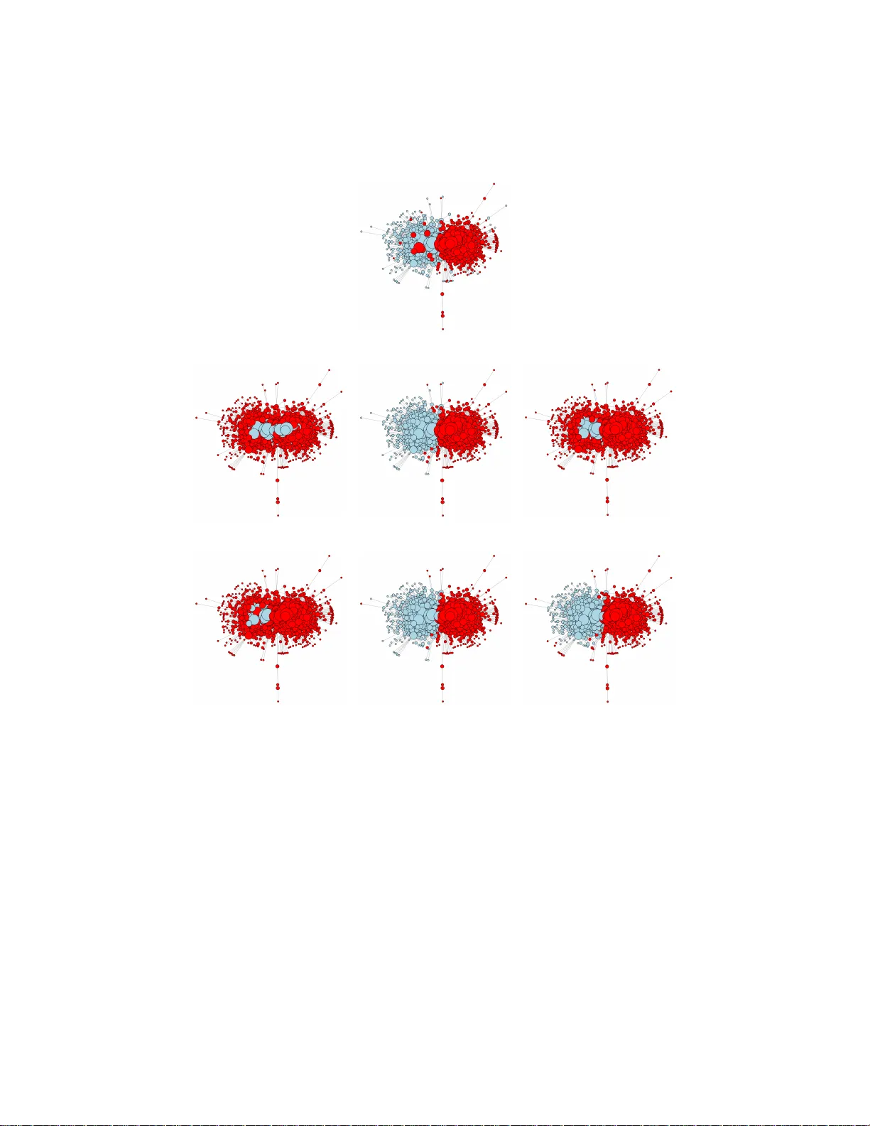
OPTIMIZA TION VIA LO W-RANK APPR O XIMA TION F OR COMMUNITY DETECTION IN NETW ORKS By Can M. Le, Eliza vet a Levina, and R oman Vershynin University of Michigan Comm unity detection is one of the fundamental problems of net- w ork analysis, for which a num b er of metho ds hav e b een proposed. Most mo del-based or criteria-based methods hav e to solve an opti- mization problem ov er a discrete set of lab els to ﬁnd communities, whic h is computationally infeasible. Some fast sp ectral algorithms ha ve b een proposed for sp eciﬁc methods or models, but only on a case-b y-case basis. Here w e propose a general approac h for maximiz- ing a function of a netw ork adjacency matrix ov er discrete lab els by pro jecting the set of labels on to a subspace appro ximating the leading eigen vectors of the exp ected adjacency matrix. This pro jection onto a low-dimensional space mak es the feasible set of labels muc h smaller and the optimization problem muc h easier. W e prov e a general result ab out this metho d and sho w how to apply it to several previously prop osed communit y detection criteria, establishing its consistency for lab el estimation in each case and demonstrating the fundamen- tal connection b etw een spectral prop erties of the netw ork and v ar- ious mo del-based approaches to comm unity detection. Simulations and applications to real-world data are included to demonstrate our metho d p erforms well for m ultiple problems ov er a wide range of parameters. 1. In tro duction. Net w orks are studied in a wide range of ﬁelds, in- cluding so cial psychology , so ciology , physics, computer science, probability , and statistics. One of the fundamen tal problems in netw ork analysis, and one of the most studied, is detecting net w ork comm unit y structure. Comm unit y detection is the problem of inferring the latent lab el vector c ∈ { 1 , . . . , K } n for the n no des from the observ ed n × n adjacency matrix A , speciﬁed by A ij = 1 if there is an edge from i to j , and A ij = 0 otherwise. While the problem of c ho osing the num ber of communities K is important, in this pa- p er we assume K is given, as do es most of the existing literature. W e fo cus on the undirected netw ork case, where the matrix A is symmetric. Roughly sp eaking, the large recent literature on communit y detection in this scenario has follow ed one of tw o trac ks: ﬁtting probabilistic mo dels for the adjacency AMS 2000 subje ct classiﬁc ations: Primary 62E10; secondary 62G05 Keywor ds and phr ases: Comm unity detection, Spectral clustering, Stochastic blo c k mo del, Social net w orks 1 2 LE ET AL. matrix A , or optimizing global criteria deriv ed from other considerations o v er lab el assignments c , often via sp ectral approximations. One of the simplest and most popular probabilistic models for ﬁtting comm unit y structure is the sto c hastic blo c k mo del (SBM) [ 17 ]. Under the SBM, the label v ector c is assumed to be dra wn from a m ultinomial distribu- tion with parameter π = { π 1 , . . . , π K } , where 0 ≤ π k ≤ 1 and P K k =1 π k = 1. Edges are then formed independently betw een every pair of nodes ( i, j ) with probabilit y P c i c j , and the K × K matrix P = [ P kl ] con trols the probabil- it y of edges within and b et w een communities. Th us the lab els are the only no de information aﬀecting edges b et ween no des, and all the nodes within the same communit y are sto c hastically equiv alen t to each other. This rules out the commonly encoun tered “h ub” nodes, whic h are no des of un usually high degrees that are connected to man y members of their o wn communit y , or simply to man y no des across the netw ork. T o address this limitation, a re- laxation that allo ws for arbitrary exp ected node degrees within comm unities w as proposed b y [ 20 ]: the degree-corrected sto c hastic block mo del (DCSBM) has P ( A ij = 1) = θ i θ j P c i c j , where θ i ’s are “degree parameters” satisfying some identiﬁabilit y constraints. In the “null” case of K = 1, b oth the blo c k mo del and the degree corrected blo c k mo del corresp ond to well-studied ran- dom graph mo dels, the Erd¨ os-R ´ enyi graph [ 10 ] and the conﬁguration mo del [ 8 ], resp ectiv ely . Man y other netw ork mo dels ha v e b een prop osed to capture the communit y structure, for example, the latent space model [ 16 ] and the laten t p osition cluster model [ 15 ]. There has also b een work on extensions of the SBM whic h allo w nodes to b elong to more than one comm unit y [ 2 , 4 , 44 ]. F or a more complete review of netw ork mo dels, see [ 13 ]. Fitting mo dels such as the sto chastic block mo del t ypically inv olv es max- imizing a likelihoo d function ov er all p ossible lab el assignmen ts, which is in principle NP-hard. MCMC-t yp e and v ariational metho ds hav e b een pro- p osed, see for example [ 41 , 35 , 25 ], as w ell as maximizing proﬁle likelihoo ds b y some type of greedy lab el-switc hing algorithms. The proﬁle lik eliho od w as derived for the SBM by [ 6 ] and for the DCSBM by [ 20 ], but the lab el- switc hing greedy search algorithms only scale up to a few thousand no des. [ 3 ] prop osed a muc h faster pseudo-likelihoo d algorithm for ﬁtting b oth these mo dels, which is based on compressing A into blo c k sums and mo deling them as a P oisson mixture. Another fast algorithm for the blo c k mo del based on b elief propagation has b een proposed by [ 9 ]. Both these algorithms rely hea vily on the particular form of the SBM likelihoo d and are not easily generalizable. The SBM likelihoo d is just one example of a function that can b e opti- mized o ver all possible no de lab els in order to p erform comm unity detection. OPTIMIZA TION VIA LOW-RANK APPRO XIMA TION 3 Man y other functions ha ve b een prop osed for this purpose, often not tied to a generative net w ork mo del. One of the b est-kno wn such functions is mo dularit y [ 33 , 31 ]. The key idea of mo dularit y is to compare the observed net w ork to a null model that has no comm unit y structure. T o deﬁne this, let e b e an n -dimensional lab el vector, n k ( e ) = P n i =1 I { e i = k } the num b er of no des in comm unity k , (1) O kl ( e ) = n X i,j =1 A ij I { e i = k , e j = l } the n um b er of edges b et ween communities k and l , k 6 = l , and O k = P K l =1 O kl the sum of no de degrees in comm unity k . Let d i = P n j =1 A ij b e the degree of no de i , and m = P n i =1 d i b e (t wice) the total num b er of edges in the graph. The Newman-Girv an mo dularit y is derived by comparing the ob- serv ed n umber of edges within communities to the num b er that w ould be exp ected under the Ch ung-Lu mo del [ 8 ] for the en tire graph, and can b e written in the form (2) Q N G ( e ) = 1 2 m X k ( O kk − O 2 k m ) The quantities O kl and O k turn out to b e the k ey comp onen t of man y com- m unit y detection criteria. The proﬁle lik eliho ods of the SBM and DCSBM discussed ab o ve can b e expressed as Q B M ( e ) = K X k,l =1 O kl log O kl n k n l , (3) Q DC ( e ) = K X k,l =1 O kl log O kl O k O l . (4) Another example is the extraction criterion [ 45 ] to extract one comm u- nit y at a time, allowing for arbitrary structure in the remainder of the net- w ork. The main idea is to recognize that some no des ma y not b elong to an y comm unity , and the strength of a communit y should dep end on ties b et ween its members and ties to the outside world, but not on ties b et w een non-mem b ers. This criterion is therefore not symmetric with respect to com- m unities, unlike the criteria previously discussed, and has the form (using sligh tly diﬀeren t notation due to lack of symmetry), (5) Q E X ( V ) = | V || V c |  O ( V ) | V | 2 − B ( V ) | V || V c |  , 4 LE ET AL. where V is the set of no des in the comm unity to b e extracted, V c is the com- plemen t of V , O ( V ) = P i,j ∈ V A ij , B ( V ) = P i ∈ V ,j ∈ V c A ij . The only known metho d for optimizing this criterion is through greedy lab el switc hing, suc h as the tabu search algorithm [ 12 ]. F or all these metho ds, ﬁnding the exact solution requires optimizing a function of the adjacency matrix A ov er all K n p ossible lab el v ectors, which is an infeasible optimization problem. In another line of work, sp ectral de- comp ositions hav e b een used in v arious wa ys to obtain approximate solutions that are muc h faster to compute. One suc h algorithm is spectral clustering (see, for example, [ 34 ]), a generic clustering metho d which b ecame p opular for communit y detection. In this context, the metho d has b een analyzed b y [ 39 , 7 , 38 , 22 ], among others, while [ 18 ] prop osed a sp ectral metho d sp ecif- ically for the DCSBM. In sp ectral clustering, t ypically one ﬁrst computes the normalized Laplacian matrix L = D − 1 / 2 AD − 1 / 2 , where D is a diagonal matrix with diagonal entries being no de degrees d i , though other normaliza- tions and no normalization at all are also p ossible (see [ 40 ] for an analysis of wh y normalization is b eneﬁcial). Then the K eigen v ectors of the Laplacian corresp onding to the ﬁrst K largest eigenv alues are computed, and their ro ws clustered using K -means into K clusters corresp onding to diﬀeren t la- b els. It has been sho wn that sp ectral clustering performs b etter with further regularization, namely if a small constant is added either to D [ 7 , 37 ] or to A [ 3 , 19 , 21 ]. The con tribution of our pap er is a new general metho d of optimizing a general function f ( A, e ) (satisfying some conditions) ov er lab els e . W e start by pro jecting the en tire feasible set of lab els onto a low-dimensional subspace spanned b y vectors appro ximating the leading eigenv ectors of E A . Pro jecting the feasible set of lab els on to a lo w-dimensional space reduces the n um b er of p ossible solutions (extreme points) from exp onen tial to polyno- mial, and in particular from O (2 n ) to O ( n ) for the case of tw o comm unities, th us making the optimization problem muc h easier. This approac h is dis- tinct from sp ectral clustering since one can sp ecify an y ob jective function f to be optimized (as long as it satisﬁes some fairly general conditions), and th us applicable to a wide range of netw ork problems. It is also distinct from initializing a search for the maxim um of a general function with the spectral clustering solution, since even with a go od initializion the feasible space W e sho w ho w our method can b e applied to maximize the likelihoo ds of the sto c hastic blo c k mo del and its degree-corrected v ersion, Newman-Girv an mo dularit y , and communit y extraction, which all solv e diﬀerent netw ork problems. While sp ectral approximations to some speciﬁc criteria that can otherwise b e only maximized b y a searc h o ver lab els ha v e been obtained on a OPTIMIZA TION VIA LOW-RANK APPRO XIMA TION 5 case-b y-case basis [ 31 , 38 , 32 ], ours is, to the b est of our kno wledge, the ﬁrst general metho d that would apply to an y function of the adjacency matrix. In this pap er, w e mainly fo cus on the case of tw o communities ( K = 2). F or metho ds that are run recursiv ely , such as mo dularit y and comm unity extraction, this is not a restriction. F or the sto c hastic blo c k mo del, the case K = 2 is of sp ecial interest and has received a lot of atten tion in the probabilit y literature (see [ 29 ] for recent adv ances). An extension to the general case of K > 2 is brieﬂy discussed in Section 2.3 . The rest of the pap er is organized as follows. In Section 2 , we set up notation and describ e our general approac h to solving a class of optimiza- tion problems ov er lab el assignments via pro jection onto a lo w-dimensional subspace. In Section 3 , w e sho w ho w the general metho d can b e applied to sev eral communit y detection criteria. Section 4 compares numerical p erfor- mance of diﬀerent metho ds. The pro ofs are giv en in the App endix. 2. A general metho d for optimization via low-rank appro xima- tion. T o start with, consider the problem of detection K = 2 communities. Man y communit y detection metho ds rely on maximizing an ob jective func- tion f ( A, e ) ≡ f A ( e ) ov er the set of no de lab els e , which can tak e v alues in, sa y , {− 1 , 1 } . Since A can be thought of as a noisy realization of E [ A ], the “ideal” solution corresp onds to maximizing f E [ A ] ( e ) instead of maximizing f A ( e ). F or a natural class of functions f describ ed b elow, f E [ A ] ( e ) is essen- tially a function o v er the set of pro jections of lab els e onto the subspace spanned b y eigen v ectors of E [ A ] and p ossibly some other constan t v ectors. In many cases E [ A ] is a low-rank matrix, which mak es f E [ A ] ( e ) a function of only a few v ariables. It is then muc h easier to inv estigate the b eha vior of f E [ A ] ( e ), which typically ac hiev es its maximum on the set of extreme p oin ts of the con v ex h ull generated by the pro jection of the lab el set e . F urther, most of the 2 n p ossible lab el assignmen ts e b ecome interior p oin ts after the pro jection, and in fact the num b er of extreme p oin ts is at most poly- nomial in n (see Remark 2.2 below); in particular, when pro jecting onto a t w o-dimensional subspace, the n umber of extreme points is of order O ( n ). Therefore, w e can ﬁnd the maximum simply b y p erforming an exhaustive searc h ov er the lab els corresponding to the extreme p oints. Section 3.5 pro- vides an alternativ e metho d to the exhaustiv e search, whic h is faster but appro ximate. In realit y , we do not kno w E [ A ], so w e need to appro ximate its columns space using the data A instead. Let U A b e an m × n matrix computed from A such that the ro w space of U A appro ximates the column space of E [ A ] (the c hoice of m × n rather than n × m is for notational con v enience that will 6 LE ET AL. b ecome apparent b elo w). Existing w ork on sp ectral clustering giv es us mul- tiple option for how to compute this matrix, e.g., using the eigenv ectors of A itself, of its Laplacian, or of their v arious regularizations – see Section 2.1 for further discussion of this issue. The algoritm w orks as follows: 1. Compute the appro ximation U A from A . 2. Find the lab els e asso ciated with the extreme p oin ts of the pro jection U A [ − 1 , 1] n . 3. Find the maximum of f A ( e ) by p erforming an exhaustive searc h ov er the set of lab els found in step 2. Note that the ﬁrst step of replacing eigen v ectors of E [ A ] with certain v ec- tors computed from A is v ery similar to sp ectral clustering. Lik e in sp ectral clustering, the output of the algorithm do es not change if w e replace U A with U A R for any orthogonal matrix R . How ever, this is where the similar- it y ends, b ecause instead of following the dimension reduction b y an ad-ho c clustering algorithm like K -means, we maximize the original ob jective func- tion. The problem is made feasible b y reducing the set of lab els ov er which to maximize, to a particular subset found b y taking into account the speciﬁc b eha vior of f E [ A ] ( e ) and f A ( e ). While our goal in the context of communit y detection is to compare f A ( e ) to f E [ A ] ( e ), the results and the algorithm in this section apply in a general settingwhere A ma y b e an y deterministic symmetric matrix. T o emphasize this generalit y , w e write all the results in this section for a generic matrix A and a generic lo w-rank matrix B , ev en though we will later apply them to the adjacency matrix A and B = E [ A ]. Let A and B b e n × n symmetric matrices with en tries b ounded by an absolute constant, and assume B has rank m  n . Assume that f A ( e ) has the general form (6) f A ( e ) = κ X j =1 g j ( h A,j ( e )) , where g j are scalar functions on R and h A,j ( e ) are quadratic forms of A and e , namely (7) h A,j ( e ) = ( e + s j 1 ) T A ( e + s j 2 ) . Here κ is a ﬁxed num b er, s j 1 and s j 2 are constan t v ectors in {− 1 , 1 } n . Note that by ( 10 ), the n umber of edges betw een communities has the form ( 7 ), and by ( 11 ), the log-likelihoo d of the degree-corrected blo ck mo del Q DC is a sp ecial case of ( 6 ) with g j ( x ) = ± x log x , x > 0. W e similarly deﬁne f B OPTIMIZA TION VIA LOW-RANK APPRO XIMA TION 7 and h B ,j , by replacing A with B in ( 6 ) and ( 7 ). By allowing e to take v alues on the cub e [ − 1 , 1] n , w e can treat h and f as functions ov er [ − 1 , 1] n . Let U B b e the m × n matrix whose ro ws are the m leading eigen v ectors of B . F or an y e ∈ [ − 1 , 1] n , U A e and U B e are the co ordinates of the pro jections of e onto the row spaces of U A and U B , respectively . Since h B ,j are quadratic forms of B and e and B is of rank m , h B ,j ’s dep end on e through U B e only , and therefore f B also dep ends on e only through U B e . In a slight abuse of notation, w e also use h B ,j and f B to denote the corresponding induced functions on U B [ − 1 , 1] n . Let E A and E B denote the subsets of lab els e ∈ {− 1 , 1 } n corresp onding to the sets of extreme p oin ts of U A [ − 1 , 1] n and U B [ − 1 , 1] n , resp ectiv ely . The output of our algorithm is (8) e ∗ = argmax  f A ( e ) , e ∈ E A  . Our goal is to get a b ound on the diﬀerence betw een the maxima of f A and f B that can b e expressed through some measure of diﬀerence betw een A and B themselv es. In order to do this, we make the follo wing assumptions. ( 1 ) F unctions g j are contin uously diﬀerentiable and there exists M 1 > 0 suc h that | g 0 j ( t ) | ≤ M 1 log( t + 2) for t ≥ 0. ( 2 ) F unction f B is con v ex on U B [ − 1 , 1] n . Assumption (1) essen tially means that Lipschitz constan ts of g j do not gro w faster than log( t + 2). The con vexit y of f B in assumption (2) ensures that f B ac hiev es its maxim um on U B E B . In some cases (see Section 3 ), the conv exity of f B can b e replaced with a weak er condition, namely the conv exit y along a certain direction. Let c ∈ {− 1 , 1 } n b e the maximizer of f B o v er the set of lab el v ectors {− 1 , 1 } n . As a function on U B [ − 1 , 1] n , f B ac hiev es its maxim um at U B ( c ), whic h is an extreme p oin t of U B [ − 1 , 1] n b y assumption (2). Lemma 2.1 pro vides a upp er b ound for f A ( c ) − f A ( e ∗ ). Throughout the pap er, we write k · k for the l 2 norm (i.e., Euclidean norm on vectors and the sp ectral norm on matrices), and k · k F for the F rob enius norm on matrices. Note that for label vectors e, c ∈ {− 1 , 1 } n , k e − c k 2 is four times the num b er of no des on which e and c diﬀer. Lemma 2.1 . If assumptions (1) and (2) hold then ther e exists a c onstant M 2 > 0 such that (9) f T ( c ) − f T ( e ∗ ) ≤ M 2 n log ( n )  k B k · k U A − U B k + k A − B k  , wher e T is either A or B . 8 LE ET AL. The pro of of Lemma 2.1 is given in App endix A . T o get a b ound on k c − e ∗ k , w e need further assumptions on B and f B . ( 3 ) There exists M 3 > 0 such that for any e ∈ {− 1 , 1 } n , k c − e k 2 ≤ M 3 √ n k U B ( c ) − U B ( e ) k . ( 4 ) There exists M 4 > 0 such that for any x ∈ U B [ − 1 , 1] n f B ( U B ( c )) − f B ( x ) k U B ( c ) − x k ≥ max f B − min f B M 4 √ n . Assumption (3) rules out the existence of multiple lab el vectors with the same pro jection U B ( c ). Assumption (4) implies that the slop e of the line connecting t w o p oin ts on the graph of f B at U B ( c ) and at an y x ∈ U B [ − 1 , 1] n is bounded from below. Thus, if f B ( x ) is close to f B ( U B ( c )) then x is also close to U B ( c ). These assumptions are satisﬁed for all functions considered in Section 3 . Theorem 2.2 . If assumptions (1)–(4) hold, then ther e exists a c onstant M 5 such that 1 n k e ∗ − c k 2 ≤ M 5 n log n  k B k · k U A − U B k + k A − B k  max f B − min f B . Theorem 2.2 follo ws directly from Lemma 2.1 and Assumptions (3) and (4). When A is a random matrix, B = E [ A ], and U A con tains the lead- ing eigen v ectors of A , a standard bound on k A − B k can b e applied (see Lemma B.2 ), whic h in turn yields a b ound on k U A − U B k b y the Da vis-Kahan Theorem. Under certain conditions, the upper b ound in Theorem 2.2 is of order o ( n ) (see Section 3 ), which sho ws consistency of e ∗ as an estimator of c (i.e., the fraction of mislab eled no des go es to 0 as n → ∞ ). 2.1. The choic e of low r ank appr oximation. An imp ortant step of our metho d is replacing the “population” space U B with the “data” approxima- tion U A . As a motiv ating example, consider the case of the SBM, with A the net w ork adjacency matrix and B = E [ A ]. When the net w ork is relativ ely dense, eigenv ectors of A are go o d estimates of the eigen vectors of B = E [ A ] (see [ 36 ] and [ 22 ] for recent improv ed error bounds). Th us, U A can just b e tak en to b e the leading eigenv ectors of A . How ev er, when the net work is sparse, this is not necessarily the b est choice, since the leading eigenv ectors of A tend to lo calize around high degree nodes, while leading eigenv ectors of the Laplacian of A tend to localize around small connected comp onen ts OPTIMIZA TION VIA LOW-RANK APPRO XIMA TION 9 [ 27 , 7 , 37 , 21 ]. This can b e av oided b y regularizing the Laplacian in some form; we follo w the algorithm of [ 3 ]; see also [ 19 , 21 ] for theoretical analysis. This w orks for b oth dense and sparse netw orks. The regularization w orks as follo ws. W e ﬁrst add a small constan t τ to eac h en try of A , and then appro ximate U B through the Laplacian of A + τ 11 T as follo ws. Let D τ b e the diagonal matrix whose diagonal en tries are sums of entries of columns of A + τ 11 T , L τ = D − 1 / 2 τ ( A + τ 11 T ) D − 1 / 2 τ , and u i b e leading eigen vectors of L τ , 1 ≤ i ≤ K . Since A + τ 11 T = D 1 / 2 τ L τ D 1 / 2 τ , w e set the app o ximation U A the b e the basis of the span of { D 1 / 2 u i : 1 ≤ i ≤ K } . F ollowing [ 3 ], w e set τ = ε ( λ n /n ), where λ n is the no de exp ected degree of the net work and ε ∈ (0 , 1) is a constant whic h has little impact on the p erformance [ 3 ]. 2.2. Computational c omplexity. Since w e prop ose an exhaustive search o v er the pro jected set of extreme points, the computational feasibilit y of this is a concern. A pro jection of the unit cub e U A [ − 1 , 1] n is the Mink owski sum of n segmen ts in R m , which, b y [ 14 ], implies that it has O ( n m − 1 ) vertices of U A [ − 1 , 1] n and they can b e found in O ( n m ) arithmetic op erations. When m = 2, which is the primary focus of our pap er, there exists an algorithm that can ﬁnd the vertices of U A [ − 1 , 1] n in O ( n log n ) arithmetic op erations [ 14 ]. Informally , the algorithm ﬁrst sorts the angles b et ween the x -axis and column v ectors of U A and − U A . It then starts at a vertex of U A [ − 1 , 1] n with the smallest y -co ordinate, and based on the order of the angles, ﬁnds neigh b or vertices of U A [ − 1 , 1] n in a coun ter-clo c kwise order. If the angles are distinct (whic h occurs with high probabilit y), mo ving from one v ertex to the next causes exactly one entry of the corresp onding label v ector to c hange the sign, and therefore the v alues of h A,j ( e ) in ( 7 ) can be up dated eﬃcien tly . In particular, if A is the adjacency matrix of a netw ork with a v erage degree λ n , then on a v arage, each update tak es O ( λ n ) arithmetic operations, and giv en U A , it only takes O ( nλ n log n ) arithmetic op erations to ﬁnd e ∗ in ( 8 ). Th us the computational complexit y of this search for t wo comm unities is not at all prohibitive – compare to the computational complexity of ﬁnding U A itself, whic h is at least O ( nλ n log n ) for m = 2. 2.3. Extension to mor e than two c ommunities. Let K b e the num b er of communities and S b e an n × K lab el matrix: for 1 ≤ i ≤ n , if no de i b elongs to communit y k then S ik = 1 and S il = 0 for all l 6 = k . The n um b ers of edges b et ween comm unities deﬁned b y ( 1 ) are entries of S T AS . Let B = P K i =1 ρ i ¯ u i ¯ u T i deﬁne the eigendecomposition of B . The population 10 LE ET AL. v ersion of S T AS is S T B S = S T   K X j =1 ρ j ¯ u j ¯ u T j   S = K X j =1 ρ j  S T ¯ u j   S T ¯ u j  T . Let U B b e the K × n matrix whose rows are ¯ u T j . Then S T B S is a function of U B S . W e appro ximate U B b y U A describ ed in Section 2.1 . Let ˜ S be the the ﬁrst K − 1 columns of S . Note that the rows of S sum to one, therefore U A S can be recov ered from U A ˜ S . No w relax the entries of ˜ S to tak e v alues in [0 , 1], with the row sums of at most one. F or 1 ≤ i ≤ n and 1 ≤ j ≤ K − 1, denote b y V ij the K × ( K − 1) matrix such that the j -th column of V ij is the i -th column of U A and all other columns are zero. Then U A ˜ S = n X i =1 K − 1 X j =1 ˜ S ij V ij . Since P K − 1 j =1 ˜ S ij ≤ 1, P K − 1 j =1 ˜ S ij V ij is a conv ex set in R K × ( K − 1) , isomorphic to a K − 1 simplex. Thus, U A ˜ S is a Mink owski sum of n conv ex sets in R K × ( K − 1) . Similar to the case K = 2, we can ﬁrst ﬁnd the set of lab el matrices ˜ S corresp onding to the extreme points of U A ˜ S and then perform the exhaustiv e searc h o v er that set. A b ound on the n umber of vertices of U A ˜ S and a polynomial algorithm to ﬁnd them are derived b y [ 14 ]. If d = K ( K − 1), then the num b er of v ertices of U A ˜ S is at most O  n ( d − 1) K 2( d − 1)  , and they can b e found in O  n d K (2 d − 1)  arithmetic op erations. presents An implemen tation of the reverse-searc h al- gorithm of [ 11 ] for computing the Minko wski sum of polytop es was presented in [ 42 ] , who sho w ed that the algorithm can b e parallelized eﬃcien tly . W e do not pursue thes e improv emen ts here, since our main fo cus in this pap er is the case K = 2. 3. Applications to comm unit y detection. Here w e apply the gen- eral results from Section 2 to a netw ork adjacency matrix A , B = E [ A ], and functions corresp onding to sev eral p opular comm unity detection criteria. Our goal is to show that our maximization metho d gets an estimate close to the true label vector c , whic h is the maximizer of the corresp onding function with B = E [ A ] plugged in for A . W e fo cus on the case of tw o comm unities and use m = 2 for the lo w rank appro ximation. Recall the quantities O 11 , O 22 , and O 12 deﬁned in ( 1 ), whic h are used b y all the criteria we consider. They are quadratic forms of A and e and can be OPTIMIZA TION VIA LOW-RANK APPRO XIMA TION 11 written as O 11 ( e ) = 1 4 ( 1 + e ) T A ( 1 + e ) , O 22 ( e ) = 1 4 ( 1 − e ) T A ( 1 − e ) , (10) O 12 ( e ) = 1 4 ( 1 + e ) T A ( 1 − e ) , where 1 is the all-ones vector. 3.1. Maximizing the likeliho o d of the de gr e e-c orr e cte d sto chastic blo ck mo del. When a netw ork has tw o communities, ( 4 ) takes the form Q DC ( e ) = O 11 log O 11 + O 22 log O 22 + 2 O 12 log O 12 (11) − 2 O 1 log O 1 − 2 O 2 log O 2 . Th us, Q DC has the form deﬁned by ( 6 ). F or simplicit y , instead of dra wing c from a m ultinomial distribution with parameter π = ( π 1 , π 2 ), w e ﬁx the true label v ector b y assigning the ﬁrst ¯ n 1 = nπ 1 no des to communit y 1 and the remaining ¯ n 2 = nπ 2 no des to comm unit y 2. Let r b e the out-in probabilit y ratio, and (12) P = λ n  1 r r ω  b e the probability matrix. W e assume that the no de degree parameters θ i are an i.i.d. sample from a distribution with E [ θ i ] = 1 and 1 /ξ ≤ θ i ≤ ξ for some constan t ξ ≥ 1. The adjacency matrix A is symmetric and for i > j has indep enden t entries generated b y A ij = Bernoulli( θ i θ j P c i c j ). Throughout the pap er, we let λ n dep end on n , and ﬁx r , ω , π , and ξ . Since λ n and the net w ork exp ected node degree are of the same order, in a slight abuse of notation, w e also denote by λ n the net w ork exp ected no de degree. Theorem 3.1 establishes consistency of our metho d in this setting. Theorem 3.1 . L et A b e the adjac ency matrix gener ate d fr om the DCSBM with λ n gr owing at le ast as log 2 n as n → ∞ . L et U A b e an appr oximation of U E [ A ] , and e ∗ the lab el ve ctor deﬁne d by ( 8 ) with f A = Q DC . Then for any δ ∈ (0 , 1) , ther e exists a c onstant M = M ( r, ω , π , ξ , δ ) > 0 such that with pr ob ability at le ast 1 − δ , we have 1 n k c − e ∗ k 2 ≤ M log n  λ − 1 / 2 n + k U A − U E [ A ] k  . In p articular, if U A is a matrix whose r ow ve ctors ar e le ading eignve ctors of A , then the fr action of mis-cluster e d no des is b ounde d by M log n/ √ λ n . 12 LE ET AL. Note that assumption (2) is diﬃcult to chec k for Q DC but a weak er ver- sion, namely conv exity along a certain direction, is suﬃcient for proving Theorem 3.1 . The pro of of Theorem 3.1 consists of chec king assumptions (1), (3), (4), and a w eak er v ersion of assumption (2). F or details, see Ap- p endix C.1 . 3.2. Maximizing the likeliho o d of the sto chastic blo ck mo del. While the regular SBM is a sp ecial case of DCSBM when θ i = 1 for all i , its lik eli- ho od is diﬀerent and thus maximizing it gives a diﬀerent solution. With t w o comm unities, ( 3 ) admits the form Q B M ( e ) = Q DC ( e ) + 2 O 1 log O 1 n 1 + 2 O 2 log O 2 n 2 , where n 1 = n 1 ( e ) and n 2 = n 2 ( e ) are the num b ers of no des in t wo commu- nities and can b e written as (13) n 1 = 1 2 ( 1 + e ) T 1 = 1 2 ( n + e T 1 ) , n 2 = 1 2 ( 1 − e ) T 1 = 1 2 ( n − e T 1 ) . Theorem 3.2 . L et A b e the adjac ency matrix gener ate d fr om the SBM with λ n gr owing at le ast as log 2 n as n → ∞ . L et U A b e an appr oximation of U E [ A ] , and e ∗ the lab el ve ctor deﬁne d by ( 8 ) with f A = Q B M . Then for any δ ∈ (0 , 1) , ther e exists a c onstant M = M ( r, ω , π , ξ , δ ) > 0 such that with pr ob ability at le ast 1 − n − δ , we have 1 n k c − e ∗ k 2 ≤ M log n  λ − 1 / 2 n + k U A − U E [ A ] k  . In p articular, if U A is a matrix whose r ow ve ctors ar e le ading eignve ctors of A , then the fr action of mis-cluster e d no des is b ounde d by M log n/ √ λ n . Note that Q B M do es not hav e the exact form of ( 6 ) but a small mod- iﬁcation shows that Lemma 2.1 still holds for Q B M . Also, assumption (2) is diﬃcult to c hec k for Q B M but again a weak er condition of conv exit y along a certain direction is suﬃcient for pro ving Theorem 3.2 . The pro of of Theorem 3.2 consists of sho wing the analog of Lemma 2.1 , c hec king as- sumptions (3), (4), and a w eaker v ersion of assumption (2). F or details, see App endix C.2 . 3.3. Maximizing the Newman–Girvan mo dularity. When a net w ork has t w o communities, up to a constan t factor the mo dularit y ( 2 ) takes the form Q N G ( e ) = O 11 + O 22 − O 2 1 + O 2 2 O 1 + O 2 = 2 O 1 O 2 O 1 + O 2 − 2 O 12 . OPTIMIZA TION VIA LOW-RANK APPRO XIMA TION 13 Again, Q N G do es not ha ve the exact form ( 6 ), but with a small modiﬁcation, the argumen t used for pro ving Lemma 2.1 and Theorem 2.2 still holds for Q N G under the regular SBM. Theorem 3.3 . L et A b e the adjac ency matrix gener ate d fr om the SBM with λ n gr owing at le ast as log n as n → ∞ . L et U A b e an appr oximation of U E [ A ] , and e ∗ the lab el ve ctor deﬁne d by ( 8 ) with f A = Q N G . Then for any δ ∈ (0 , 1) , ther e exists a c onstant M = M ( r, ω , π , ξ , δ ) > 0 such that with pr ob ability at le ast 1 − n − δ , we have 1 n k c − e ∗ k 2 ≤ M  λ − 1 / 2 n + k U A − U E [ A ] k  . In p articular, if U A is a matrix whose r ow ve ctors ar e le ading eignve ctors of A , then the fr action of mis-cluster e d no des is b ounde d by M / √ λ n . It is easy to see that Q N G is Lipsc hitz with resp ect to O 1 , O 2 , and O 12 , whic h is stronger than assumption (1) and ensures the pro of of Lemma 2.1 go es through. The pro of of Theorem 3.3 consists of chec king assumptions (2), (3), (4), and the Lipsc hitz condition for Q N G . F or details, see Appendix C.3 . 3.4. Maximizing the c ommunity extr action criterion. Iden tifying the com- m unit y V to b e extracted with a lab el vector e , the criterion ( 5 ) can b e written as Q E X ( e ) = n 2 n 1 O 11 − O 12 , where n 1 , n 2 are deﬁned b y ( 13 ). Once again Q E X do es not ha ve the ex- act form ( 6 ), but with small mo diﬁcations of the pro of, Lemma 2.1 and Theorem 2.2 still hold for Q E X . Theorem 3.4 . L et A b e the adjac ency matrix gener ate d fr om the SBM with the pr ob ability matrix ( 12 ) , ω = r , and λ n gr owing at le ast as log n as n → ∞ . L et U A b e an appr oximation of U E [ A ] , and e ∗ the lab el ve ctor deﬁne d by ( 8 ) with f A = Q E X . Then for any δ ∈ (0 , 1) , ther e exists a c onstant M = M ( r , ω , π , ξ , δ ) > 0 such that with pr ob ability at le ast 1 − n − δ , we have 1 n k c − e ∗ k 2 ≤ M  λ − 1 / 2 n + k U A − U E [ A ] k  . In p articular, if U A is a matrix whose r ow ve ctors ar e le ading eignve ctors of A , then the fr action of mis-cluster e d no des is b ounde d by M / √ λ n . The proof of Theorem 3.4 consists of verifying a version of Lemma 2.1 and assumptions (2), (3), and (4), and is included in App endix C.4 . 14 LE ET AL. 3.5. An alternative to exhaustive se ar ch. While the pro jected feasible space is m uch smaller than the original space, w e may still w an t to av oid the exhaustive search for e ∗ in ( 8 ). The geometry of the pro jection of the cub e can b e used to deriv e an appro ximation to e ∗ that can b e computed without a search. −20 −15 −10 −5 0 5 10 15 20 −20 −15 −10 −5 0 5 10 15 20 n 1 = n 2 = 150 λ = 15 , r = 0 . 2 Fig 1 . The pr oje ction of the cub e [ − 1 , 1] n onto two-dimensional subsp ace. Blue c orr esp onds to the pr oje ction onto eigenve ctors of A , and r e d onto the eigenvectors of E [ A ] . The r e d c ontour is the boundary of U E [ A ] [ − 1 , 1] n ; the blue dots are the extr eme p oints of U A [ − 1 , 1] n . Cir cles (at the c orners) ar e ± pr oj e ctions of the true lab el vector; squar es ar e ± pr oje ctions of the ve ctor of al l 1s. Recall that U E [ A ] is an 2 × n matrix whose rows are the leading eigenv ec- tors of E [ A ], and U A appro ximates U E [ A ]. F or SBM, it is easy to see that U E [ A ] [ − 1 , 1] n , the pro jection of the unit cub e on to the tw o leading eigen- v ectors of U E [ A ] , is a parallelogram with vertices {± U E [ A ] 1 , ± U E [ A ] c } , where 1 ∈ R n is a v ector of all 1s (see Lemma C.1 in the supplemen t). W e can then expect the pro jection U A [ − 1 , 1] n to look somewhat similar – see the illustration in Figure 1 . Note that ± U E [ A ] c are the farthest points from the line connecting the other t wo v ertices, U E [ A ] 1 and − U E [ A ] 1 . Motiv ated by this observ ation, w e can estimate c by ˆ c = arg max n h U A e, ( U A 1 ) ⊥ i : e ∈ {− 1 , 1 } n o (14) = sign( u T 1 1 u 2 − u T 2 1 u 1 ) , where U A = ( u 1 , u 2 ) T and ( U A 1 ) ⊥ is the unit vector p erp endicular to U A 1 . Note that ˆ c depends on U A only , not on the ob jectiv e function, a prop- ert y it shares with spectral clustering. Ho w ever, ˆ c pro vides a deterministic estimate of the lab els based on a geometric prop ert y of U A , while sp ec- tral clustering uses K -means, which is iterativ e and typically depends on OPTIMIZA TION VIA LOW-RANK APPRO XIMA TION 15 a random initialization. Using this geometric approximation allows us to a v oid b oth the exhaustiv e search and the iterations and initialization of K -means, although it ma y not alw ays b e as accurate as the search. When the communit y detection problem is relativ ely easy , we exp ect the geomet- ric appro ximation to perform w ell, but when the problem b ecomes harder, the exhaustiv e searc h should pro vide b etter results. This intuition is con- ﬁrmed by simulations in Section 4 . Theorem 3.5 shows that ˆ c is a consistent estimator. The pro of is giv en in App endix B . Theorem 3.5 . L et A b e an adjac ency matrix gener ate d fr om the SBM with λ n gr owing at le ast as log n as n → ∞ . L et U A b e an appr oximation to U E [ A ] . Then for any δ ∈ (0 , 1) ther e exists M = M ( r , ω , π , ξ , δ ) > 0 such that with pr ob ability at le ast 1 − n − δ , we have 1 n k ˆ c − c k 2 ≤ M k U A − U E [ A ] k 2 . In p articular, if U A is a matrix whose r ow ve ctors ar e le ading eignve ctors of A , then the fr action of mis-cluster e d no des is b ounde d by M /λ n . 3.6. The or etic al c omp arisons. There are s ev eral results on the consis- tency of recov ering the true lab el v ector under b oth the SBM and the DCSBM. The balanced planted partition mo del G ( n, a n , b n ), which is the simplest sp ecial case of the SBM, has received m uch attention recently , es- p ecially in the probability literature. This mo del assumes that there are tw o comm unities with n/ 2 no des eac h, and edges are formed within comm uni- ties and b et w een comm unities with probabilities a/n and b/n , resp ectively . When ( a − b ) 2 ≤ 2( a + b ), no method can ﬁnd the comm unities [ 28 ]. Al- gorithms based on non-backtrac king random walks that can recov er the comm unit y structure b etter than random guessing if ( a − b ) 2 > 2( a + b ) ha v e b een prop osed in [ 30 , 26 ] Moreov er, if ( a − b ) 2 / ( a + b ) → ∞ as n → ∞ then the fraction of mis-clustered no des go es to zero with high probabilit y . Under the mo del G ( n, a n , b n ), our theoretical results require that a + b grows at least as log n . This matches the requiremen ts on the exp ected degree λ n needed for consistency in [ 6 ] for the SBM and in [ 46 ] for the DCSBM. When the exp ected no de degree λ n is of order log n , sp ectral clustering using eigen vectors of the adjacency matrix can correctly reco ver the com- m unities, with fraction of mis-clustered no des up to O (1 / log n ) [ 22 ]. In this regime, our method for maximizing the Newman-Girv an and the commu- nit y extraction criteria mis-clusters at most O (1 / √ λ n ) fraction of the nodes. F or maximizing the lik eliho ods of the SBM and DCSBM, w e require that λ n is of order log 2 n , and the fraction of mis-clustered no des is b ounded b y 16 LE ET AL. O (log n/ √ λ n ). F or Newman-Girv an modularity as well as the SBM lik eli- ho od, [ 6 ] prov ed strong consistency (p erfect recov ery with high probabil- it y) under the SBM when λ n gro ws faster than log n . Ho w ev er, they used a lab el-switc hing algorithm for ﬁnding the maximizer, which is computa- tionally infeasible for larger netw orks. A muc h faster algorithm based on pseudo-lik eliho od w as prop osed by [ 3 ], who assumed that the initial esti- mate of the lab els (obtained in practice by regularized sp ectral clustering) has a certain correlation with the truth, and show ed that the fraction of mis-clustered no des for their metho d is O (1 /λ n ). Recently , [ 21 ] analyzed regularized spectral clustering in the sparse regime when λ n = O (1), and sho w ed that with high probability , the fraction of mis-clustered no des is O (log 6 λ n /λ n ). In summary , our assumptions required for consistency are similar to others in the literature even though the approximation metho d is fairly general. 4. Numerical comparisons. Here we brieﬂy compare the empirical p erformance of our extreme p oin t pro jection metho d to sev eral other meth- o ds for comm unity detection, both general (sp ectral clustering) and those designed sp eciﬁcally for optimizing a particular communit y detection cri- terion, using both simulated netw orks and t wo real net work datasets, the p olitical blogs and the dolphins data describ ed in in Section 4.5 . Our goal in this comparison is to sho w that our general method do es as w ell as the algorithms tailored to a particular criterion, and th us we are not trading oﬀ accuracy for generality . F or the four criteria discussed in Section 3 , w e compare our metho d of maximizing the relev ant criterion by exhaustive search ov er the extreme p oin ts of the pro jection (EP , for extreme p oints), the approximate version based on the geometry of the feasible set desc ribed in Section 3.5 (AEP , for approximate extreme p oin ts), and regularized sp ectral clustering (SCR) prop osed by [ 3 ], which are all general metho ds. W e also include one metho d sp eciﬁc to the criterion in each comparison. F or the SBM, we compare to the unconditional pseudo-lik eliho od (UPL) and for the DCSBM, to the con- ditional pseudo-lik eliho od (CPL), tw o fast and accurate metho ds dev elop ed sp eciﬁcally for these mo dels by [ 3 ]. F or the Newman-Girv an mo dularity , w e compare to the sp ectral algorithm of [ 31 ], whic h uses the leading eigenv ector of the mo dularity matrix (see details in Section 4.3 ). Finally , for comm unit y extraction w e compare to the algorithm prop osed in the original pap er [ 45 ] based on greedy lab el switc hing, as there are no faster algorithms a v ailable. The sim ulated net works are generated using the parametrization of [ 3 ], as follo ws. Throughout this section, the num b er of no des in the netw ork OPTIMIZA TION VIA LOW-RANK APPRO XIMA TION 17 is ﬁxed at n = 300, the n umber of comm unities K = 2, and the true lab el v ector c is ﬁxed. The n umber of replications for each setting is 100. First, the no de degree parameters θ i are dra wn indep enden tly from the distribution P (Θ = 0 . 2) = γ , and P (Θ = 1) = 1 − γ . Setting γ = 0 gives the standard SBM, and γ > 0 giv es the DCSBM, with 1 − γ the fraction of hub no des. The matrix of edge probabilities P is con trolled b y t wo parameters: the out-in probabilit y ratio r , whic h determines ho w lik ely edges are formed within and b et ween comm unities, and the weigh t v ector w = ( w 1 , w 2 ), whic h determines the relativ e no de degrees within comm unities. Let P 0 =  w 1 r r w 2  . The diﬃcult y of the problem is largely con trolled by r and the o v erall ex- p ected net w ork degree λ . Thus w e rescale P 0 to con trol the exp ected degree, setting P = λP 0 ( n − 1)( π T P 0 π )( E [Θ]) 2 , where π = n − 1 ( n 1 , n 2 ), and n k is the n um b er of no des in comm unity k . Finally , edges A ij are dra wn indep enden tly from a Bernoulli distribution with P ( A ij = 1) = θ i θ j P c i c j . As discussed in Section 2.1 , a go od approximation to the eigenv ectors of E [ A ] is pro vided b y the eigenv ectors of the regularized Laplacian. SCR uses these eigenv ectors u 1 , u 2 as input to K -means (computed here with the kmeans function in Matlab with 40 random initial starting p oints). EP and AEP use { D 1 / 2 u 1 , D 1 / 2 u 2 } to compute the matrix U A (see Section 2.1 ). T o ﬁnd extreme p oin ts and corresp onding lab el v ectors in the second step of EP , w e use the algorithm of [ 14 ]. F or m = 2, it essen tially consists of sorting the angles of b et w een the column vectors of U A and the x -axis. In case of m ultiple maximizers, w e break the tie b y c ho osing the label vector whose pro jection is the farthest from the line connecting the pro jections of ± 1 (follo wing the geometric idea of Section 3.5 ). F or CPL and UPL, follo wing [ 3 ], w e initialize with the output of SCR and set the n um b er of outer iterations to 20. W e measure the accuracy of all methods via the normalized m utual in- formation (NMI) b et ween the label vector c and its estimate e . NMI takes v alues b et w een 0 (random guessing) and 1 (perfect match), and is deﬁned b y [ 43 ] as NMI( c, e ) = − P i,j R ij log R ij R i + R + j  P ij R ij log R ij  − 1 , where R is the confusion matrix b etw een c and e , which represen ts a biv ariate prob- abilit y distribution, and its row and column sums R i + and R + j are the corresp onding marginals. 18 LE ET AL. 0 0.1 0.2 0.3 0.4 0.4 0.6 0.8 1 NMI r w = (1 , 1) 0 0.1 0.2 0.3 0.4 0.4 0.6 0.8 1 NMI r w = (1 , 3) 0.4 0.6 0.8 1 SCR AEP EP[DC] CPL NMI w = (1 , 1) , r = 0 . 3 0.4 0.6 0.8 1 SCR AEP EP[DC] CPL NMI w = (1 , 3) , r = 0 . 3 SCR AEP EP[DC ] CPL SCR AEP EP[DC ] CPL Fig 2 . The de gr e e-c orr e cte d sto chastic blo ck mo del. T op r ow: b oxplots of NMI b etween true and estimate d lab els. Bottom r ow: aver age NMI against the out-in pr ob ability r atio r . In al l plots, n 1 = n 2 = 150 , λ = 15 , and γ = 0 . 5 . 4.1. The de gr e e-c orr e cte d sto chastic blo ck mo del. Figure 2 shows the per- formance of the four metho ds for ﬁtting the DCSBM under diﬀeren t param- eter settings. W e use the notation EP[DC] to emphasize that EP here is used to maximize the log-likelihoo d of DCSBM. In this case, all metho ds p erform similarly , with EP performing the b est when communit y-level degree w eights are diﬀerent ( w = (1 , 3)), but just slightly w orse than CPL when w = (1 , 1). The AEP is alwa ys somewhat w orse than the exact version, esp ecially when w = (1 , 3), but o verall their results are comparable. 4.2. The sto chastic blo ck mo del. Figure 3 shows the p erformance of the four metho ds for ﬁtting the regular SBM ( γ = 0). Over all, four metho ds pro vide quite similar results, as we w ould hope goo d ﬁtting methods will. The p erformance of the app o ximate metho d AEP is v ery similar to that of EP , and the mo del-speciﬁc UPL marginally outp erforms the three general metho ds. 4.3. Newman–Girvan mo dularity. The mo dularity function ˆ Q N G can b e appro ximately maximized via a fast sp ectral algotithm when partitioning in to t wo communities [ 31 ]. Let B = A − P where P ij = d i d j /m , and write ˆ Q N G ( e ) = 1 2 m e T B e . The approximate solution (LES, for leading eigen vector signs) assigns no de labels according to the signs of the corresp onding entries of the leading eigenv ector of B . F or a fair comparison to other metho ds relying on eigen vectors, w e also use the regularized A + τ 11 T instead of A OPTIMIZA TION VIA LOW-RANK APPRO XIMA TION 19 0 0.1 0.2 0.3 0.4 0.4 0.6 0.8 1 NMI r w = (1 , 1) 0 0.1 0.2 0.3 0.4 0.4 0.6 0.8 1 NMI r w = (1 , 3) 0.4 0.6 0.8 1 SCR AEP EP[BM] UPL NMI w = (1 , 1) , r = 0 . 3 0.4 0.6 0.8 1 SCR AEP EP[BM] UPL NMI w = (1 , 3) , r = 0 . 3 SCR AEP EP[BM] UPL SCR AEP EP[BM] UPL Fig 3 . The sto chastic block mo del. T op r ow: b oxplots of NMI b etwe en true and estimate d lab els. Bottom r ow: aver age NMI against the out-in pr ob ability r atio r . In al l plots, n 1 = n 2 = 150 , λ = 15 , and γ = 0 . here, since empirically we found that it sligh tly improv es the p erformance of LES. Figure 4 sho ws the p erformance of AEP , EP[NG], and LES, when the data are generated from a regular blo c k model ( γ = 0). The t wo extreme p oin t metho ds EP[NG] and AEP b oth do sligh tly better than LES, esp ecially for the un balanced case of w = (1 , 3), and there is essentially no diﬀerence b et ween EP[NG] and AEP here. 4.4. Community extr action criterion. F ollowing the original extraction pap er of [ 45 ], we generate a communit y with background from the regular blo c k mo del with K = 2, n 1 = 60, n 2 = 240, and the probabilit y matrix prop ortional to P 0 =  0 . 4 0 . 1 0 . 1 0 . 1  . Th us, no des within the ﬁrst comm unity are tigh tly connected, while the rest of the no des ha v e equally w eak links with all other no des and represent the bac kground. W e consider four v alues for the a v erage exp ected no de degree, 15, 20, 25, and 30. Figure 5 sho ws that EP[EX] p erforms better than SCR and AEP , but somewhat w orse than the greedy lab el-switc hing tabu searc h used in the original pap er for maximizing the comm unity extraction criterion (TS). How ev er, the tabu search is v ery computationally in tensiv e and only feasible up to p erhaps a thousand no des, so for larger netw orks it is not an option at all, and no other method has been previously prop osed for this 20 LE ET AL. 0 0.1 0.2 0.3 0.4 0.4 0.6 0.8 1 NMI r w = (1 , 1) 0 0.1 0.2 0.3 0.4 0.4 0.6 0.8 1 NMI r w = (1 , 3) 0.4 0.6 0.8 1 LES AEP EP[NG] NMI w = (1 , 1) , r = 0 . 3 0.4 0.6 0.8 1 LES AEP EP[NG] NMI w = (1 , 3) , r = 0 . 3 LES AEP EP[NG] LES AEP EP[NG] Fig 4 . Newman-Girvan mo dularity. T op r ow: b oxplots of NMI b etwe en true and estimate d lab els. Bottom r ow: aver age NMI against the out-in pr ob ability r atio r . In al l plots, n 1 = n 2 = 150 , λ = 15 , and γ = 0 . problem. The AEP metho d, whic h do es not agree with AE as w ell as in the other cases, probably suﬀers from the inherent assymetry of the extraction problem. 0 0.2 0.4 0.6 0.8 1 SCR AEP EP[EX] TS NMI λ = 15 0 0.2 0.4 0.6 0.8 1 SCR AEP EP[EX] TS NMI λ = 20 0 0.2 0.4 0.6 0.8 1 SCR AEP EP[EX] TS NMI λ = 25 0 0.2 0.4 0.6 0.8 1 SCR AEP EP[EX] TS NMI λ = 30 Fig 5 . Community extr action. The b oxplots of NMI b etwe en true and estimate d lab els. In al l plots, n 1 = 60 , n 2 = 240 , and γ = 0 . OPTIMIZA TION VIA LOW-RANK APPRO XIMA TION 21 4.5. R e al-world network data. The ﬁrst net w ork w e test our metho ds on, assem bled by [ 1 ], consists of blogs ab out US p olitics and h yp erlinks betw een blogs. Each blog has b een manually lab eled as either lib eral or conserv ative, whic h we use as the ground truth. F ollowing [ 20 ], and [ 46 ], w e ignore direc- tions of the h yp erlinks and only examine the largest connected comp onen t of this netw ork, which has 1222 no des and 16,714 edges, with the av erage degree of appro ximately 27. T able 1 and Figure 6 show the p erformance of diﬀeren t methods. While AEP , EP[DC], and CPL giv e reasonable results, SCR, UPL, and EP[BM] clearly miscluster the nodes. This is consisten t with previous analyses whic h sho wed that the degree correction has to b e used for this net work to achiev e the correct partition, b ecause of the presense of h ub no des. T able 1 The NMI b etwe en true and estimate d lab els for r eal-world networks. Metho d SCR AEP EP[BM] EP[DC] UPL CPL Blogs 0.290 0.674 0.278 0.731 0.001 0.725 Dolphins 0.889 0.814 0.889 0.889 0.889 0.889 The second netw ork we study represen ts so cial ties b et ween 62 b ottlenose dolphins living in Doubtful Sound, New Zealand [ 24 , 23 ]. At some p oin t during the study , one well-connected dolphin (SN100) left the group, and the group split in to t wo separate parts, which w e use as the ground truth in this example. T able 1 and Figure 7 show the p erformance of diﬀerent metho ds. In Figure 7 , no de shap es represen t the actual split, while the colors represen t the estimated lab el. The star-shap ed no de is the dolphin SN100 that left the group. Excepting that dolphin, SCR, EP[BM], EP[DC], UPL, and CPL all miscluster one node, while AEP misclusters tw o no des. Since this small net w ork can b e well mo delled b y the SBM, there is no diﬀerence b et ween DCSBM and SBM based metho ds, and all metho ds p erform w ell. Ac kno wledgmen ts. W e thank the Asso ciate Editor and three anony- mous referees for detailed and constructive feedback which led to many impro v ements. W e also thank Y unp eng Zhao (George Mason Universit y) for sharing his co de for the tabu searc h, and Arash A. Amini (UCLA) for sharing his code for the pseudo-lik eliho od metho ds and helpful discussions. E.L. is partially supp orted b y NSF grants DMS-01106772 and DMS-1159005. R.V. is partially supported b y NSF grants DMS 1161372, 1001829, 1265782 and USAF Gran t F A9550-14-1-0009. 22 LE ET AL. (a) T rue Lab els (b) UPL (c) CPL (d) SCR (e) EP(BM) (f ) EP(DC) (g) AEP Fig 6 . The network of p olitic al blo gs. No de diameter is pr op ortional to the lo garithm of its de gr e e and the c olors r epr esent c ommunity lab elss. References. [1] Adamic, L. A. and Glance, N. (2005). The p olitical blogosphere and the 2004 US election. In Pr o c e edings of the WWW-2005 Workshop on the Weblo gging Ec osystem . [2] Airoldi, E. M., Blei, D. M., Fien b erg, S. E., and Xing, E. P . (2008). Mixed membership sto c hastic blockmodels. J. Machine L e arning R ese ar ch , 9:1981–2014. [3] Amini, A., Chen, A., Bick el, P ., and Levina, E. (2013). Fitting comm unity mo dels to large sparse net works. A nnals of Statistics , 41(4):2097–2122. [4] Ball, B., Karrer, B., and Newman, M. E. J. (2011). An eﬃcien t and principled method for detecting comm unities in netw orks. Physic al R eview E , 34:036103. OPTIMIZA TION VIA LOW-RANK APPRO XIMA TION 23 (a) AEP ● ● ● ● ● ● ● ● ● ● ● ● ● ● ● ● ● ● ● ● ● ● ● ● ● ● ● ● ● ● ● ● ● ● ● ● ● ● ● ● ● Beak Beescratch Bumper CCL Cross DN16 DN21 DN63 Double Feather Fish Five Fork Gallatin Grin Haecksel Hook Jet Jonah Knit Kringel MN105 MN23 MN60 MN83 Mus Notch Number1 Oscar Patchback PL Quasi Ripplefluke Scabs Shmuddel SMN5 SN100 SN4 SN63 SN89 SN9 SN90 SN96 Stripes Thumper T opless TR120 TR77 TR82 TR88 TR99 Trigger TSN103 TSN83 Upbang V au W ave W eb Whitetip Zap Zig Zipfel (b) SCR, EP , UPL, CPL ● ● ● ● ● ● ● ● ● ● ● ● ● ● ● ● ● ● ● ● ● ● ● ● ● ● ● ● ● ● ● ● ● ● ● ● ● ● ● ● ● Beak Beescratch Bumper CCL Cross DN16 DN21 DN63 Double Feather Fish Five Fork Gallatin Grin Haecksel Hook Jet Jonah Knit Kringel MN105 MN23 MN60 MN83 Mus Notch Number1 Oscar Patchback PL Quasi Ripplefluke Scabs Shmuddel SMN5 SN100 SN4 SN63 SN89 SN9 SN90 SN96 Stripes Thumper T opless TR120 TR77 TR82 TR88 TR99 Trigger TSN103 TSN83 Upbang V au W ave W eb Whitetip Zap Zig Zipfel Fig 7 . The network of 62 b ottlenose dolphins. No de shap es r epr esent the split after the dol- phin SN100 (r epr esente d by the star) left the gr oup. No de c olors r epr esent their estimate d lab els. [5] Bhatia, R. (1996). Matrix Analysis . Springer-V erlag New Y ork. [6] Bick el, P . J. and Chen, A. (2009). A nonparametric view of net work mo dels and Newman-Girv an and other mo dularities. Pr o c. Natl. A c ad. Sci. USA , 106:21068–21073. [7] Chaudhuri, K., Ch ung, F., and Tsiatas, A. (2012). Sp ectral clustering of graphs with general degrees in the extended planted partition mo del. Journal of Machine L e arning R ese ar ch Workshop and Confer enc e Pr o c e edings , 23:35.1 – 35.23. [8] Chung, F. and Lu, L. (2002). Connected components in random graphs with given degree sequences. Annals of Combinatorics , 6:125–145. [9] Decelle, A., Krzak ala, F., Mo ore, C., and Zdeborov´ a, L. (2012). Asymptotic analysis of the sto chastic blo c k mo del for mo dular netw orks and its algorithmic applications. Physic al R eview E , 84:066106. [10] Erd˝ os, P . and R´ enyi, A. (1959). On random graphs. I. Publ. Math. Debre c en , 6:290– 297. [11] F ukuda, K. (2004). F rom the zonotop e construction to the minko wski addition of con vex polytop es. Journal of Symb olic Computation , 38(4):1261–1272. [12] Glov er, F. W. and Lagunas, M. (1997). T abu se ar ch . Klu wer Academic. [13] Goldenberg, A., Zheng, A. X., Fienberg, S. E., and Airoldi, E. M. (2010). A surv ey of statistical netw ork mo dels. F oundations and T r ends in Machine L e arning , 2:129–233. [14] Gritzmann, P . and Sturmfels, B. (1993). Mink owski addition of p olytopes: com- putational complexity and applications to Grobner bases. SIAM Journal on Discr ete Mathematics , 6(2):246–269. [15] Handco c k, M. D., Raftery , A. E., and T an trum, J. M. (2007). Mo del-based clustering for so cial netw orks. J. R. Statist. So c. A , 170:301–354. [16] Hoﬀ, P . D., Raftery , A. E., and Handco c k, M. S. (2002). Latent space approaches to so cial netw ork analysis. Journal of the Americ an Statistic al Asso ciation , 97:1090–1098. [17] Holland, P . W., Laskey , K. B., and Leinhardt, S. (1983). Sto chastic blo c kmo dels: ﬁrst steps. So cial Networks , 5(2):109–137. [18] Jin, J. (2015). F ast netw ork communit y detection by score. The Annals of Statistics , 24 LE ET AL. 43(1):57–89. [19] Joseph, A. and Y u, B. (2013). Impact of regularization on sp ectral clustering. arXiv:1312.1733 . [20] Karrer, B. and Newman, M. E. J. (2011). Stochastic blo c kmo dels and communit y structure in net works. Physic al R eview E , 83:016107. [21] Le, C. M., Levina, E., and V ersh ynin, R. (2015). Sparse random graphs: regularization and concentration of the Laplacian. . [22] Lei, J. and Rinaldo, A. (2015). Consistency of spectral clustering in sparse sto c hastic blo c k models. The Annals of Statistics , 43(1):215–237. [23] Lusseau, D. and Newman, M. E. J. (2004). Identifying the role that animals pla y in their so cial netw orks. Pr o c. R. Soc. L ondon B (Suppl.) , 271:S477–S481. [24] Lusseau, D., Schneider, K., Boisseau, O. J., Haase, P ., Slooten, E., and Dawson, S. M. (2003). The bottlenose dolphin comm unity of doubtful sound features a large propor- tion of long-lasting asso ciations. can geographic isola- tion explain this unique trait? Behavior al Ec olo gy and So ciobiolo gy , 54:396–405. [25] Mariadassou, M., Robin, S., and V ac her, C. (2010). Uncov ering laten t structure in v alued graphs: A v ariational approach. The A nnals of Applie d Statistics , 4(2):715–742. [26] Massouli´ e, L. (2014). Comm unity detection thresholds and the w eak Ramanujan prop ert y . In Pr o c e edings of the 46th A nnual ACM Symp osium on The ory of Computing , STOC ’14, pages 694–703. [27] Mihail, M. and Papadimitriou, C. H. (2002). On the eigenv alue p o wer la w. Pr o ce e dings of the 6th Inter ational Workshop on R andomization and Appr oximation T e chniques , pages 254–262. [28] Mossel, E., Neeman, J., and Sly , A. (2012). Stochastic block models and reconstruc- tion. [29] Mossel, E., Neeman, J., and Sly , A. (2014a). Belief propagation, robust reconstruc- tion, and optimal reco very of blo c k mo dels. COL T , 35:356–370. [30] Mossel, E., Neeman, J., and Sly , A. (2014b). A pro of of the blo c k mo del threshold conjecture. . [31] Newman, M. E. J. (2006). Finding communit y structure in net works using the eigen- v ectors of matrices. Physic al R eview E , 74(3):036104. [32] Newman, M. E. J. (2013). Sp ectral methods for net work comm unit y detection and graph partitioning. Physic al R eview E , 88:042822. [33] Newman, M. E. J. and Girv an, M. (2004). Finding and ev aluating communit y struc- ture in net works. Physic al R eview E , 69(2):026113. [34] Ng, A., Jordan, M., and W eiss, Y. (2001). On sp ectral clustering: Analysis and an al- gorithm. In Dietterich, T., Bec ker, S., and Ghahramani, Z., editors, Neur al Information Pr o c essing Systems 14 , pages 849–856. MIT Press. [35] Nowic ki, K. and Snijders, T. A. B. (2001). Estimation and prediction for stochastic blo c kstructures. Journal of the A meric an Statistic al Asso ciation , 96(455):1077–1087. [36] O’Rourke, S., V u, V., and W ang, K. (2013). Random perturbation of low rank matrices: Improving classical b ounds. . [37] Qin, T. and Rohe, K. (2013). Regularized sp ectral clustering under the degree- corrected sto c hastic blo c kmo del. In A dvanc es in Neur al Information Pr o c essing Sys- tems , pages 3120–3128. [38] Riolo, M. and Newman, M. E. J. (2012). First-principles m ultiw ay sp ectral parti- tioning of graphs. . [39] Rohe, K., Chatterjee, S., and Y u, B. (2011). Sp ectral clustering and the high- dimensional sto c hastic blo c k mo del. Annals of Statistics , 39(4):1878–1915. [40] Sark ar, P . and Bic k el, P . (2013). Role of normalization in spectral clustering for OPTIMIZA TION VIA LOW-RANK APPRO XIMA TION 25 sto c hastic blockmodels. . [41] Snijders, T. and Nowic ki, K. (1997). Estimation and prediction for sto chastic blo ck- structures for graphs with latent blo c k structure. Journal of Classiﬁc ation , 14:75–100. [42] W eibel, C. (2010). Implemen tation and parallelization of a rev erse-search algorithm for Minko wski sums. Pr o c e e dings of the 12th Workshop on Algorithm Engine ering and Exp eriments , pages 34–42. [43] Y ao, Y. Y. (2003). Information-theoretic measures for knowledge discov ery and data mining. In Entr opy Me asur es, Maximum Entr opy Principle and Emer ging Applic ations , pages 115–136. Springer. [44] Zhang, Y., Levina, E., and Zhu, J. (2014). Detecting ov erlapping communities in net works using sp ectral metho ds. . [45] Zhao, Y., Levina, E., and Zh u, J. (2011). Communit y extraction for social netw orks. Pr o c. Natl. A c ad. Sci. USA , 108(18):7321–7326. [46] Zhao, Y., Levina, E., and Zhu, J. (2012). Consistency of comm unit y detection in net- w orks under degree-corrected sto c hastic block models. Annals of Statistics , 40(4):2266– 2292. APPENDIX A: PR OOF OF RESUL TS IN SECTION 2 The following Lemma bounds the Lipschitz constants of h B ,j and f B on U B [ − 1 , 1] n . Lemma A.1 . Assume that Assumption ( 1 ) holds. F or any j ≤ κ (se e 6 ), and x, y ∈ U B [ − 1 , 1] n , we have   h B ,j ( x ) − h B ,j ( y )   ≤ 4 √ n k B k · k x − y k ,   f B ( x ) − f B ( y )   ≤ M √ n log ( n ) k B k · k x − y k , wher e M is a c onstant indep endent of n . Proof of Lemma A.1 . Let e, s ∈ [ − 1 , 1] n suc h that x = U B e, y = U B s and denote L =   h B ,j ( x ) − h B ,j ( y )   . Then L =   ( e + s j 1 ) T B ( e + s j 2 ) − ( s + s j 1 ) T B ( s + s j 2 )   =   e T B ( e − s ) + ( e − s ) T B s + ( s j 2 + s j 1 ) T B ( e − s )   ≤ 4 √ n k B ( e − s ) k . Let B = P m i =1 ρ i u i u T i b e the eigendecomp osition of B . Then k B ( e − s ) k 2 =    m X i =1 ρ i u i u T i ( e − s )    2 =    m X i =1 ρ i ( x i − y i ) u i    2 = m X i =1 ρ 2 i ( x i − y i ) 2 ≤ k B k 2 m X i =1 ( x i − y i ) 2 = k B k 2 · k x − y k 2 . 26 LE ET AL. Therefore L ≤ 4 √ n k B k · k x − y k . Since h B ,j are quadratic, they are of order O ( n 2 ). Hence by Assumption (1), the Lipschitz constants of g j are of order log( n ). Therefore   f B ( x ) − f B ( y )   ≤ 4 √ n log ( n ) k B k · k x − y k , whic h completes the pro of. In the follo wing proofs w e use M to denote a p ositiv e constant indep en- den t of n the v alue of which may change from line to line. Proof of Lemma 2.1 . Since k e + s j 1 k ≤ 2 √ n and k e + s j 2 k ≤ 2 √ n , | h A,j ( e ) − h B ,j ( e ) | = | ( e + s j 1 ) T ( A − B )( e + s j 2 ) | ≤ 4 n k A − B k . Since h A,j and h B ,j are of order O ( n 2 ), g 0 j are b ounded b y log ( n ). T ogether with assumption (1) it implies that there exists M > 0 such that (15) | f A ( e ) − f B ( e ) | ≤ M n log ( n ) k A − B k . Let ˆ e = arg max { f B ( e ) , e ∈ E A } . Then f A ( e ∗ ) ≥ f A ( ˆ e ) and b y ( 15 ) we get f B ( ˆ e ) − f B ( e ∗ ) ≤ f B ( ˆ e ) − f A ( ˆ e ) + f A ( e ∗ ) − f B ( e ∗ ) (16) ≤ M n log( n ) k A − B k . Denote b y conv( S ) the con v ex hull of a set S . Then U A c ∈ conv( U A E A ) and therefore, there exists η e ≥ 0, P e ∈E A η e = 1 suc h that U A c = X e ∈E A η e U A ( e ) = U A  X e ∈E A η e e  . Hence dist  U B c, conv( U B E A )  ≤    U B c − U B  X e ∈E A η e e     (17) =    ( U B − U A ) c + ( U A − U B ) X e ∈E A η e e    ≤ 2 √ n k U A − U B k . Let y ∈ conv( U B E A ) b e the closest p oin t from conv( U B E A ) to U B c , i.e. k U B c − y k = dist  U B c, conv( U B E A )  . OPTIMIZA TION VIA LOW-RANK APPRO XIMA TION 27 By 17 and Lemma A.1 , we ha ve (18) f B ( U B c ) − f B ( y ) ≤ M n log( n ) k B k · k U A − U B k . The con v exit y of f B implies that f B ( y ) ≤ f B ( U B ˆ e ), and in turn, (19) f B ( U B c ) − f B ( U B ˆ e ) ≤ M n log( n ) k B k · k U A − U B k . Note that f B ( U B e ) = f B ( e ) for ev ery e ∈ [ − 1 , 1] n . Adding ( 16 ) and ( 19 ), we get ( 9 ) for T = B . The case T = A then follows from ( 15 ) b ecause replacing B with A induces an error which is not greater than the upper b ound of ( 9 ) for T = B . APPENDIX B: PR OOF OF THEOREM 6 W e ﬁrst present the closed form of eigen v alues and eigenv ectors of E [ A ] under the regular blo c k mo dels. Lemma B.1 . Under the SBM, the nonzer o eigenvalues ρ i and c orr e- sp onding eigenve ctors ¯ u i of E [ A ] have the fol lowing form. F or i = 1 , 2 , ρ i = λ n 2 h ( π 1 + π 2 ω ) + ( − 1) i − 1 p ( π 1 + π 2 ω ) 2 − 4 π 1 π 2 ( ω − r 2 ) i , ¯ u i = 1 q n ( π 1 r 2 i + π 2 ) ( r i , r i , ..., r i , 1 , 1 , ..., 1) T , wher e r i = 2 π 2 r ( π 2 ω − π 1 ) + ( − 1) i p ( π 1 + π 2 ω ) 2 − 4 π 1 π 2 ( ω − r 2 ) . The ﬁrst ¯ n 1 = nπ 1 entries of ¯ u i e qual r i  n ( π 1 r 2 i + π 2 )  − 1 / 2 and the last ¯ n 2 = nπ 2 entries of ¯ u i e qual  n ( π 1 r 2 i + π 2 )  − 1 / 2 . Proof of Lemma B.1 . Under the SBM E [ A ] is a t w o-by-t wo blo c k ma- trix with equal en tries within eac h blo c k. It is easy to v erify directly that E [ A ] ¯ u i = ρ i ¯ u i for i = 1 , 2. Lemma B.2 b ounds the diﬀerence betw een the eigenv alues and eigenv ec- tors of A and those of E [ A ] under the SBM. It also pro vides a w ay to simplify the general upp er b ound of Theorem 2.2 . Lemma B.2 . Under the SBM, let U A and U E [ A ] b e 2 × n matric es whose r ows ar e the le ading eigenve ctors of A and E [ A ] , r esp e ctively. F or any δ > 0 , 28 LE ET AL. ther e exists a c onstant M = M ( r, ω , π , δ ) > 0 such that if λ n > M log ( n ) then with pr ob ability at le ast 1 − n − δ , we have (20) k A − E [ A ] k ≤ M p λ n , (21) k U A − U E [ A ] k ≤ M √ λ n . Proof of Lemma B.2 . Inequality ( 20 ) follows directly from Theorem 5.2 of [ 22 ] and the fact that the maxim um of the exp ected no de degrees is of order λ n . Inequalit y ( 21 ) is a consequence of ( 20 ) and the Davis-Kahan theorem (see Theorem VII.3.2 of [ 5 ]) as follows. By Lemma B.1 , the nonzero eigen v alues ρ 1 and ρ 2 of ¯ A are of order λ n . Let S = h ρ 2 − M p λ n , ρ 1 + M p λ n i . Then ρ 1 , ρ 2 ∈ S and the gap b et w een S and zero is of order λ n . Let ¯ P be the pro jector onto the subspace spanned b y t wo leading eigen vectors of E [ A ]. Since λ n gro ws faster than k A − E [ A ] k b y 20 , only tw o leading eigenv alues of A b elong to S . Let P b e the pro jector onto the subspace spanned by tw o leading eigen v ectors of A . By the Davis-Kahan theorem, k U A − U E [ A ] k = k ¯ P − P k ≤ 2 k A − E [ A ] k λ n ≤ 2 M √ λ n , whic h completes the pro of. Before pro ving Theorem 3.5 we need to establish the follo wing lemma. Lemma B.3 . L et x , y , ¯ x , and ¯ y b e unit ve ctors in R n such that h x, y i = h ¯ x, ¯ y i = 0 . L et P and ¯ P b e the ortho gonal pr oje ctions on the subsp ac es sp anne d by { x, y } and { ¯ x, ¯ y } r esp e ctively. If k P − ¯ P k ≤  then ther e exists an ortho gonal matrix K of size 2 × 2 such that || ( x, y ) K − ( ¯ x, ¯ y ) || F ≤ 9  . Proof of Lemma B.3 . Let x 0 = P ¯ x and y 0 = P ¯ y . Since k P − ¯ P k ≤  , it follo ws that k ¯ x − x 0 k ≤  and k ¯ y − y 0 k ≤  . Let x ⊥ = x 0 k x 0 k , then k ¯ x − x ⊥ k ≤ k ¯ x − x 0 k + k x 0 − x ⊥ k ≤  + | 1 − k x 0 k| ≤ 2 . Also h x ⊥ , y 0 i = h x ⊥ , y 0 − ¯ y i + h x ⊥ − ¯ x, ¯ y i implies that |h x ⊥ , y 0 i| ≤ 3  . Deﬁne z = y 0 − h y 0 , x ⊥ i x ⊥ . Then h z , x ⊥ i = 0, k ¯ y − z k ≤ k ¯ y − y 0 k + k y 0 − z k ≤ 4  , and | 1 − k z k| = |k ¯ y k − k z k| ≤ 4  . Let y ⊥ = 1 k z k z , then k ¯ y − y ⊥ k ≤ k ¯ y − z k + k z − y ⊥ k ≤ 4  + | 1 − k z k| ≤ 8 . Therefore k ( ¯ x, ¯ y ) − ( x ⊥ , y ⊥ ) k F ≤ 9  . Finally , let K = ( x, y ) T ( x ⊥ , y ⊥ ). OPTIMIZA TION VIA LOW-RANK APPRO XIMA TION 29 Proof of Theorem 3.5 . Denote ε = k U A − U E [ A ] k , U = ( u 1 , u 2 ) T = U A , and ¯ U = ( ¯ u 1 , ¯ u 2 ) T = U E [ A ] . W e ﬁrst sho w that there exists a constant M > 0 such that with probabilit y at least 1 − δ , (22) min    ( u T 1 1 u 2 − u T 2 1 u 1 ) ± ( ¯ u T 1 1 ¯ u 2 − ¯ u T 2 1 ¯ u 1 )    ≤ M ε √ n. Let R =  0 − 1 1 0  b e the π / 2-rotation on R 2 . Then u T 1 1 u 2 − u T 2 1 u 1 = U T R U 1 , ¯ u T 1 1 ¯ u 2 − ¯ u T 2 1 ¯ u 1 = ¯ U T R ¯ U 1 . By Lemma B.2 and Lemma B.3 , there exists an orthogonal matrix K suc h that if E = ( E 1 , E 2 ) = U T − ¯ U T K then || E || F ≤ 9 ε . By replacing U T with E + ¯ U T K , the left hand side of ( 22 ) b ecomes min     E + ¯ U T K  R  E + ¯ U T K  T 1 ± ¯ U T R ¯ U 1    . Note that K T RK = R if K is a rotation, and K T RK = −R if K is a reﬂection. Therefore, it is enough to show that   ¯ U T KR E T 1 + E RK T ¯ U 1 + E R E T 1   ≤ M  √ n. Note that | E T i 1 | ≤ √ n k E i k ≤ 9 ε √ n and k E k F ≤ 9 ε ≤ 18, so k E R E T 1 k = k E T 2 1 E 1 − E T 1 1 E 2 k ≤ 18 2 ε √ n. F rom Lemma B.1 we see that ¯ U 1 = √ n ( s 1 , s 2 ) T for some s 1 and s 2 not dep ending on n . It follo ws that k E RK T ¯ U 1 k = √ n k ( E 2 − E 1 ) K T ( s 1 , s 2 ) T k ≤ M ε √ n for some M > 0. Analogously , k ¯ U T KR E T 1 k = k ¯ U T K ( − E T 2 1 , E T 1 1 ) T k ≤ M ε √ n, and ( 22 ) follows. By Lemma B.1 , w e hav e ¯ U T R ¯ U 1 = α ( π 2 , π 2 , ..., π 2 , − π 1 , ..., − π 1 ) T , where α does not dep end on n ; the ﬁrst n 1 en tries of ¯ U T R ¯ U 1 equal απ 2 and the last n 2 en tries of ¯ U T R ¯ U 1 equal απ 1 . F or simplicity , assume that in ( 22 ) the minimum is when the sign is negative (b ecause ˆ c is unique up to a factor of − 1). If no de i is mis-clustered by ˆ c then | ( U T R U 1 ) i − ( ¯ U T R ¯ U 1 ) i | ≥ min i | ( ¯ U T R ¯ U 1 ) i | =: η . Let k be the n umber of mis-clustered no des, then by ( 22 ), η √ k ≤ M ε √ n . Therefore the fraction of mis-clustered nodes, k/n , is of order ε 2 . If U A is formed by the leading eigen v ectors of A , then it remains to use inequalit y ( 21 ) of Lemma B.2 . 30 LE ET AL. APPENDIX C: PR OOF OF RESUL TS IN SECTION 3 Let us ﬁrst describ e the pro jection of the cub e under regular blo c k mo dels, whic h will b e used to replace Assumption (2). See Figure 1 for an illustration. Lemma C.1 . Consider the r e gular blo ck mo dels and let R = U E [ A ] [ − 1 , 1] n . Then R is a p ar al lelo gr am; the vertic es of R ar e {± U E [ A ] ( c ) , ± U E [ A ] ( 1 ) } , wher e c is a true lab el ve ctor. The angle b etwe en two adjac ent sides of R do es not dep end on n . Proof of Lemma C.1 . Eigenv ectors of E [ A ] are computed in Lemma B.1 . Let x =  r 1  n ( π 1 r 2 1 + π 2 )  − 1 / 2 , r 2  n ( π 1 r 2 2 + π 2 )  − 1 / 2  T , y =   n ( π 1 r 2 1 + π 2 )  − 1 / 2 ,  n ( π 1 r 2 2 + π 2 )  − 1 / 2  T . Then R = { (  1 + · · · +  ¯ n 1 ) x + (  ¯ n 1 +1 + · · · +  n ) y ,  i ∈ [ − 1 , 1] } , and it is easy to see that R is a parallelogram. V ertices of R corresp ond to the cases when  1 = · · · =  ¯ n 1 = ± 1 and  ¯ n 1 +1 = · · · =  n = ± 1. The angle betw een t w o adjacent sides of R equals the angle betw een √ nx and √ ny , which does not dep end on n . C.1. Pro of of results in Section 3.1 . Under degree-corrected blo ck mo dels, let us denote b y ¯ A the conditional expectation of A given the degree parameters θ = ( θ 1 , ..., θ n ) T . Note that if θ i ≡ 1 then ¯ A = E A . Since ¯ A dep ends on θ , its eigenv alues and eigenv ectors may not ha ve a closed form. Nev ertheless, we can appro ximate them using ρ i and ¯ u i from Lemma B.1 . T o do so, w e need the following lemma. Lemma C.2 . L et M = ρ 1 x 1 x T 1 + ρ 2 x 2 x T 2 , wher e x 1 , x 2 ∈ R n , k x 1 k = k x 2 k = 1 , ρ 1 6 = 0 , and ρ 2 6 = 0 . If c = h x 1 , x 2 i then the eigenvalues z i and c orr esp onding eigenve ctors y i of M have the fol lowing form. F or i = 1 , 2 , z i = 1 2 h ( ρ 1 + ρ 2 ) + ( − 1) i − 1 p ( ρ 2 − ρ 1 ) 2 + 4 ρ 1 ρ 2 c 2 i , y i = ( cρ 1 ) x 1 + ( z i − ρ 1 ) x 2 . If ρ 1 and ρ 2 ar e ﬁxe d, ρ 1 ≥ ρ 2 , and c = o (1) as n → ∞ then eigenvalues and eigenve ctors of M have the form z 1 = ρ 1 + O ( c 2 ) , z 2 = ρ 2 + O ( c 2 ) , y 1 = x 1 + O ( c ) x 2 , y 2 = x 2 + O ( c ) x 1 . OPTIMIZA TION VIA LOW-RANK APPRO XIMA TION 31 Proof of Lemma C.2 . It is easy to verify that M y i = z i y i for i = 1 , 2. The asymptotic formulas of z i and y i then follow directly from the forms of z i and y i . The next lemma sho ws the appro ximation of eigen v alues and eigen v ectors of ¯ A . Lemma C.3 . Consider the de gr e e-c orr e cte d blo ck mo dels (describ e d in Se ction 3.1 ) and let D θ = diag ( θ ) . Denote by ¯ A the c onditional exp e ctation of A given θ . Then for any δ ∈ (0 , 1) , with pr ob ability at le ast 1 − δ , the nonzer o eigenvalues ρ θ i and c orr esp onding eigenve ctors ¯ u θ i of ¯ A have the fol lowing form. F or i = 1 , 2 , ρ θ i = ρ i k D θ ¯ u i k 2 (1 + O (1 /n )) , ¯ u θ 1 = ˜ u θ 1 k ˜ u θ 1 k , wher e ˜ u θ 1 = D θ ¯ u 1 k D θ ¯ u 1 k + O  n − 1 / 2  D θ ¯ u 2 k D θ ¯ u 2 k , ¯ u θ 2 = ˜ u θ 2 k ˜ u θ 2 k , wher e ˜ u θ 2 = D θ ¯ u 2 k D θ ¯ u 2 k + O  n − 1 / 2  D θ ¯ u 1 k D θ ¯ u 1 k , wher e ρ i , ¯ u i , and r i ar e deﬁne d in L emma B.1 . Proof of Lemma C.3 . Let M = ρ 1 ¯ u 1 ¯ u T 1 + ρ 2 ¯ u 2 ¯ u T 2 b e the exp ectation of the adjacency matrix in the regular blo c k model setting. In the degree- corrected blo c k mo del setting, given θ , w e ha v e E [ A ] = D θ M D θ = ρ 1 D θ ¯ u 1 ( D θ ¯ u 1 ) T + ρ 2 D θ ¯ u 2 ( D θ ¯ u 2 ) T = ρ 1 k D θ ¯ u 1 k 2 D θ ¯ u 1 k D θ ¯ u 1 k ( D θ ¯ u 1 ) T k D θ ¯ u 1 k + ρ 2 k D θ ¯ u 2 k 2 D θ ¯ u 2 k D θ ¯ u 2 k ( D θ ¯ u 2 ) T k D θ ¯ u 2 k . W e are now in the setting of Lemma C.2 with c =  k D θ ¯ u 1 kk D θ ¯ u 2 k  − 1 h D θ ¯ u 1 , D θ ¯ u 2 i = c θ  π 1 q ( π 1 r 2 1 + π 2 )( π 1 r 2 2 + π 2 ) k D θ ¯ u 1 kk D θ ¯ u 2 k  − 1 , where c θ = 1 n  π 1 ( θ 2 ¯ n 1 +1 + · · · + θ 2 n ) − π 2 ( θ 2 1 + · · · + θ 2 ¯ n 1 )  . Note that the tw o sums in the form ula of c θ ha v e the same expectation. It remains to apply Ho eﬀding’s inequalit y to eac h sum. Since we do not ha v e closed-form form ulas for eigen vectors of ¯ A , we can not describ e U ¯ A [ − 1 , 1] n explicitly . Lemma C.4 pro vides an approximation of U ¯ A [ − 1 , 1] n . It will b e used to replace Assumption (2). 32 LE ET AL. Lemma C.4 . Consider the setting of L emma C.3 and let R θ = U ¯ A [ − 1 , 1] n and (23) ˆ R θ = con v {± U ¯ A ( c ) , ± U ¯ A ( 1 ) } . Then ˆ R θ is a p ar al lelo gr am and the angle b etwe en two adjac ent sides is b ounde d away fr om zer o and π ; R θ is wel l appr oximate d by ˆ R θ in the sense that dist  R θ , ˆ R θ  = sup x ∈R θ inf y ∈ ˆ R θ k x − y k = O (1) as n → ∞ . Proof of Lemma C.4 . Let v i = k D θ ¯ u i k − 1 D θ ¯ u i , i = 1 , 2, V = ( v 1 , v 2 ) T , and R V = V [ − 1 , 1] n . F ollo wing the same argumen t in the pro of of Lemma C.1 , it is easy to sho w that R V is a parallelogram with v ertices {± V c, ± V 1 } . By Lemma C.3 , k v i − ¯ u θ i k = O ( n − 1 / 2 ), which in turn implies dist  R θ , R V  = O (1). The distance b et w een t wo parallelograms R V and ˆ R θ is b ounded b y the maximum of the distances betw een corresp onding vertices, which is also of order O (1) b ecause k v i − ¯ u θ i k = O ( n − 1 / 2 ). Finally by triangle inequality dist  ˆ R θ , R θ  ≤ dist  ˆ R θ , R V  + dist  R V , R θ  = O (1) . The angle b etw een tw o adjacent sides of R V equals the angle b et ween √ nx and √ ny , where x and y are deﬁned in the pro of of Lemma C.1 , whic h do es not dep end on n . Since dist( ˆ R θ , R V ) = O (1), the angle b et w een tw o adjacen t sides of ˆ R θ is b ounded from zero and π . Before showing prop erties of the proﬁle log-likelihoo d, let us introduce some new notations. Let ¯ O 11 , ¯ O 12 , ¯ O 22 , and ¯ Q DC b e the p opulation v ersion of O 11 , O 12 , O 22 , and Q DC , when A is replaced with ¯ A . W e also use ¯ Q B M , ¯ Q N G , and ¯ Q E X to denote the p opulation version of Q B M , Q N G , and Q E X resp ectiv ely . The follo wing discussion is ab out ¯ Q DC , but it can b e carried out for ¯ Q B M , ¯ Q N G , and ¯ Q E X with ob vious modiﬁcations and the help of Lemma C.6 . Note that ¯ O 11 , ¯ O 12 , and ¯ O 22 are quadratic forms of e and ¯ A , therefore ¯ Q DC dep ends on e through U ¯ A e , where U ¯ A is the 2 × n matrix whose ro ws are eigen v ectors of ¯ A . With a little abuse of notation, we also use ¯ O ij , i, j = 1 , 2, and ¯ Q DC to denote the induced functions on U ¯ A [ − 1 , 1] n . Th us, for example if x ∈ U ¯ A [ − 1 , 1] n then ¯ Q DC ( x ) = ¯ Q DC ( U ¯ A e ) for an y e ∈ [ − 1 , 1] n suc h that x = U ¯ A e . OPTIMIZA TION VIA LOW-RANK APPRO XIMA TION 33 T o simplify ¯ Q DC , let ρ θ 1 and ρ θ 2 b e eigenv alues of ¯ A as in Lemma C.3 and let t = ( t 1 , t 2 ) T = U ¯ A 1 , µ = ( ρ θ 1 t 1 , ρ θ 2 t 2 ) T . W e parameterize x ∈ U ¯ A [ − 1 , 1] n b y x = αt + β v , where v = ( v 1 , v 2 ) T is a unit v ector p erp endicular to µ . If w e denote a = 1 4 ( ρ θ 1 t 2 1 + ρ θ 2 t 2 2 ) and b = 1 4 ( ρ θ 1 v 2 1 + ρ θ 2 v 2 2 ), then ¯ O 11 = ( α + 1) 2 a + β 2 b, ¯ O 22 = ( α − 1) 2 a + β 2 b, ¯ O 12 = (1 − α 2 ) a − β 2 b, ¯ O 1 = ¯ O 11 + ¯ O 12 = 2(1 + α ) a, ¯ O 2 = ¯ O 22 + ¯ O 12 = 2(1 − α ) a. Note that ¯ O 11 ¯ O 22 − ¯ O 2 12 = 4 β 2 ab > 0 since ρ θ 1 and ρ θ 2 are p ositiv e by Lemma C.3 . With a little abuse of notation, we also use ¯ Q DC ( α, β ) to denote the v alue of ¯ Q DC in the ( α, β ) coordinates describ ed ab o ve. W e no w sho w some prop erties of ¯ Q DC . Lemma C.5 . Consider ¯ Q = ¯ Q DC on ˆ R θ deﬁne d by ( 23 ) . Then ( a ) ¯ Q ( α, 0) is a c onstant. ( b ) ∂ 2 ¯ Q ∂ β 2 ≥ 0 , ∂ ¯ Q ∂ β > 0 if β > 0 and ∂ ¯ Q ∂ β < 0 if β < 0 . Thus, ¯ Q achieves minimum when β = 0 and maximum on the b oundary of ˆ R θ . ( c ) ¯ Q is c onvex on the b oundary of ˆ R θ . Thus, ¯ Q achieves maximum at ± U ¯ A ( c ) . ( d ) F or any x ∈ U ¯ A [ − 1 , 1] n , if ¯ Q ( U ¯ A ( c )) − ¯ Q ( x ) ≤  then k U ¯ A ( c ) − x k ≤ 4  √ n  ¯ Q ( U ¯ A ( c )) − min ˆ R θ ¯ Q  − 1 . ( e ) F or any δ ∈ (0 , 1) , max ˆ R θ ¯ Q − min ˆ R θ ¯ Q is of or der nλ n with pr ob ability at le at 1 − δ . P arts (a) and (b) are used to pro v e part (c), which together with Lemma C.4 will b e used to replace Assumption (2). Parts (d) v eriﬁes Assumption (4), and part (e) provides a wa y to simplify the upp er b ound in part (d). Proof of Lemma C.5 . Note that b ecause ˆ R θ ⊂ R θ , ¯ O 11 , ¯ O 12 , and ¯ O 22 are nonnegativ e on ˆ R θ . Also, if we m ultiply ¯ O 11 , ¯ O 12 , and ¯ O 22 b y a con- stan t η > 0 then the resulting function has the form η ¯ Q + C , where C is a constan t not depending on ( α, β ), and therefore the b eha vior of ¯ Q that w e are interested in do es not c hange. In this pro of we use η = 1 /a . Since ¯ Q 34 LE ET AL. is symmetric with resp ect to β , after m ultiplying by 1 /a , we replace β 2 b/a with β and only consider β ≥ 0. Thus, w e ma y assume that ¯ O 11 = ( α + 1) 2 + β , ¯ O 22 = ( α − 1) 2 + β , ¯ O 12 = (1 − α 2 ) − β , (24) ¯ O 1 = ¯ O 11 + ¯ O 12 = 2(1 + α ) , ¯ O 2 = ¯ O 22 + ¯ O 12 = 2(1 − α ) . ( a ) With ( 24 ) and β = 0, it is straightforw ard to verify that Q ( α, 0) do es not dep end on α . ( b ) Simple calculation shows that ∂ ¯ Q ∂ β = log ¯ O 11 ¯ O 22 ¯ O 2 12 ≥ 0 , ∂ 2 ¯ Q ∂ β 2 = 1 ¯ O 11 + 1 ¯ O 22 + 2 ¯ O 12 ≥ 0 . ( c ) W e show that ¯ Q is conv ex on the b oundary line connecting U ¯ A ( 1 ) and U ¯ A ( c ). Let ( α 0 , β 0 ) T b e the co ordinates of U ¯ A ( c ), where β 0 > 0 and α 0 ∈ ( − 1 , 1). W e parameterize the segment connecting U ¯ A ( c ) and U ¯ A ( 1 ) by (  α, β 0 (1 − α ) 1 − α 0  T , α ∈ [ α 0 , 1] ) . (25) With this parametrization, ¯ O 11 , ¯ O 12 , and ¯ O 22 ha v e the forms ¯ O 11 = ( α + 1) 2 + ρ ( α − 1) 2 , ¯ O 22 = ( α − 1) 2 + ρ ( α − 1) 2 ¯ O 12 = (1 − α 2 ) − ρ ( α − 1) 2 , ρ = β 2 0 (1 − α 0 ) 2 . Simple calculation shows that 1 2 d 2 ¯ Q dα 2 = ( ρ + 1) log ( ρ + 1) ¯ O 11 [ α + 1 + ρ ( α − 1)] 2 + 4 ρ [ α + 1][ α + 1 + ρ ( α − 1)] − 8 ρ ¯ O 11 . Note that the v alue of the right-hand side at α = 1 is ( ρ + 1) log( ρ + 1) − ρ ≥ 0 for any ρ ≥ 0. Therefore to sho w that d 2 ¯ Q dα 2 ≥ 0, it is enough to sho w that d 2 ¯ Q dα 2 is non-increasing. Simple calculation shows that d 3 ¯ Q dα 3 = 16 ρ 2  ( α − 1) 2 ρ + α 2 − 2 α − 3  × ×  (3 α + 1)( α − 1) ρ + 3( α + 1) 2  D − 1 , OPTIMIZA TION VIA LOW-RANK APPRO XIMA TION 35 where D = ¯ O 2 11 ( α + 1) 2 [ α + 1 + ρ ( α − 1)] 2 . Since ρ (1 − α ) ≤ (1 + α ) b ecause ¯ O 12 ≥ 0, it follo ws that ( α − 1) 2 ρ + α 2 − 2 α − 3 ≤ (1 − α )(1 + α ) + α 2 − 2 α − 3 = − 2( α + 1) ≤ 0 . Note that if (3 α + 1)( α − 1) ≥ 0 then (3 α + 1)( α − 1) ρ + 3( α + 1) 2 ≥ 0. Otherwise 3 α + 1 ≥ 0 and since ρ ( α − 1) ≥ − (1 + α ), it follo ws that (3 α + 1)( α − 1) ρ + 3( α + 1) 2 ≥ − (3 α + 1)( α + 1) + 3( α + 1) 2 = 2( α + 1) ≥ 0 . Th us d 3 ¯ Q dα 3 ≤ 0. W e hav e shown that ¯ Q is conv ex on the segment connecting U ¯ A ( c ) and U ¯ A ( 1 ). The same argumen t applies for other sides of the b oundary of ˆ R θ . ( d ) Let ( α x , β x ) b e the parameters of x , ˆ x be the p oint with parameters ( α x , 0), and x ∗ b e the p oin t on the boundary of ˆ R U with parameters ( α x , β ∗ x ). Without loss of generality we assume that x ∗ is on the line connecting x c = U ¯ A ( c ) and x 1 = U ¯ A ( 1 ). Note that ( a ),( b ), and ( c ) imply ¯ Q ( x c ) ≥ ¯ Q ( x ∗ ) ≥ ¯ Q ( x ) ≥ ¯ Q ( ˆ x ) = ¯ Q ( x 1 ) . Let ` = ¯ Q ( x c ) − min ˆ R θ ¯ Q . Since ¯ Q ( α x , β ) is conv ex in β (b y ( b )), w e ha ve k x ∗ − x k k x ∗ − ˆ x k ≤ ¯ Q ( x ∗ ) − ¯ Q ( x ) ¯ Q ( x ∗ ) − ¯ Q ( ˆ x ) ≤ ¯ Q ( x c ) − ¯ Q ( x ) ¯ Q ( x c ) − ¯ Q ( ˆ x ) ≤  ` . Therefore k x ∗ − x k ≤ ` − 1 k x ∗ − ˆ x k ≤ 2  √ n` − 1 . Since ¯ Q is con vex on the b oundary of ˆ R θ , w e ha v e k x c − x ∗ k k x c − x 1 k ≤ ¯ Q ( x c ) − ¯ Q ( x ∗ ) ¯ Q ( x c ) − ¯ Q ( x 1 ) ≤ ¯ Q ( x c ) − ¯ Q ( x ) ¯ Q ( x c ) − ¯ Q ( x 1 ) ≤  ` , whic h in turn implies k x c − x ∗ k ≤ ` − 1 k x c − x 1 k ≤ 2  √ n` − 1 . Finally by triangle inequalit y k x c − x k ≤ k x c − x ∗ k + k x ∗ − x k ≤ 4  √ n` − 1 . ( e ) Note that min ˆ R θ ¯ Q = ¯ Q ( α 0 , 0) = ¯ Q (0 , 0). Also, to ﬁnd ¯ Q ( c ) − ¯ Q (0) we do not ha ve to calculate ¯ O 1 log ¯ O 1 + ¯ O 2 log ¯ O 2 since along the line α = α 0 , ¯ O 1 and ¯ O 2 do not change. Simple calculation with Ho eﬀding’s inequality sho w that with probability at least 1 − δ the following hold ¯ O 11 (0) = ¯ O 22 (0) = ¯ O 12 (0) = nλ n 4  π 2 1 + ω π 2 2 + 2 π 1 π 2 r  + O ( λ n √ n ) , 36 LE ET AL. ¯ O 11 ( c ) = nλ n π 2 1 + ¯ O ( λ n √ n ) , ¯ O 22 ( c ) = nλ n ω π 2 2 + O ( λ n √ n ) , ¯ O 12 ( c ) = nλ n π 1 π 2 r + O ( λ n √ n ) . By the remark at the beginning of the pro of of Lemma C.5 , we can tak e η = nλ n , and therefore ¯ Q ( U ¯ A ( c )) − min ˆ R θ ¯ Q is of order nλ n . Proof of Theorem 3.1 . Note that ¯ Q = ¯ Q DC do es not satisfy all As- sumptions (1)–(4), therefore we can not apply Theorem 2.2 directly . Instead w e will follo w the idea of the pro of of Lemma 2.1 . W e ﬁrst sho w that ¯ Q satisﬁes Assumption (1). F or ¯ Q , the functions g j in ( 6 ) has the form g ( z ) = z log( z ). W e can assume that z > 1 b ecause otherwise g ( z ) is b ounded by a constant. Since g 0 ( z ) = 1 + log ( z ), g 0 ( z ) do es not gro w faster than log ( z ), and therefore assumption (1) holds. Note that by Lemma C.4 , dist  ˆ R , ˆ R θ  is b ounded by a constant; by Lemma A.1 , the Lipschitz constan t of ¯ Q is of order O  √ n log ( n ) k ¯ A k  . Therefore, to pro ve Lemma 2.1 , and in turn Theorem 3.1 , it is enough to consider ¯ Q on ˆ R θ . Note also that ¯ Q may not b e con vex, therefore Assumption (2) may not hold. But we now show that the con vexit y of ¯ Q is not needed. In the proof of Lemma 2.1 , the con vexit y of f B is used only at one place to sho w that ( 18 ) implies ( 19 ), or more sp eciﬁcally , that f B ( y ) ≤ f B ( U B ( ˆ e )). Note that b y 17 , k y − U ¯ A ( c ) k ≤ 2 √ n k U A − U ¯ A k . By Lemma C.5 part c, ¯ Q ac hieves maxim um at U ¯ A ( c ), a vertex of ˆ R θ ; by Lemma C.4 , the angle b et w een tw o adjacen t sides of ˆ R θ is b ounded aw ay from zero and π . Th us, there exists s ∈ E A suc h that k y − U ¯ A ( s ) k ≤ M √ n k U A − U ¯ A k . By Lemma A.1 we hav e | ¯ Q ( y ) − ¯ Q ( U ¯ A ( s )) | ≤ M n log ( n ) k ¯ A k · k U A − U ¯ A k . Therefore in ( 18 ) w e can replace y with U ¯ A ( s ), and ( 19 ) follo ws by deﬁnition of ˆ e . W e no w c hec k assumptions (3) and (4). T o c heck the assumption (3), w e ﬁrst assume that U ¯ A = ( D θ ( ¯ u 1 , ¯ u 2 )) T , where ¯ u 1 and ¯ u 2 are from Lemma B.1 , and D θ = diag( θ ). The ﬁrst ¯ n 1 = nπ 1 column v ectors of ( ¯ u 1 , ¯ u 2 ) T are equal and we denote by ξ 1 . The last ¯ n 2 = nπ 2 column vectors of ( ¯ u 1 , ¯ u 2 ) T are also equal and we denote by ξ 2 . Then U ¯ A ( c ) − U ¯ A ( e ) = ¯ n 1 X i =1 θ i (1 − e i ) ξ 1 + n X i = ¯ n 1 +1 θ i ( − 1 − e i ) ξ 2 = k 1 ¯ n 1 X i =1 θ i ξ 1 − k 2 n X i = ¯ n 1 +1 θ i ξ 2 , OPTIMIZA TION VIA LOW-RANK APPRO XIMA TION 37 where k 1 = P ¯ n 1 i =1 (1 − e i ), k 2 = P n i = ¯ n 1 (1 + e i ), and k e − c k 2 = k 1 + k 2 . By Lemma B.1 , entries of ξ 1 , ξ 2 are of order 1 / √ n and the angle b et ween ξ 1 , ξ 2 do es not dep end on n , it follo ws that √ n k U ¯ A ( c ) − U ¯ A ( e ) k is of order k 1 + k 2 . By Lemma C.3 , it is easy to see that the argumen t still holds for the actual U ¯ A . Assumption (4) follows directly from part ( e ) of Lemma C.5 . Com bining Assumptions (3), (4), and Lemma 2.1 , w e see that Theo- rem 2.2 holds. Note that the conclusion of Lemma B.2 still holds if w e replace E [ A ] with ¯ A , except the constan t M now also depends on ξ , that is M = M ( r, ω , π , δ ) > 0. The upp er b ound in Theorem 2.2 is simpliﬁed b y Lemma B.2 and part d of Lemma C.5 . The b ound in Theorem 2.2 is simpliﬁed b y ( 20 ) of Lemma B.2 and part e of Lemma C.5 : k e ∗ − c k 2 ≤ M n log n  λ − 1 / 2 n + k U A − U E [ A ] k  . If U A is formed by eigenv ectors of A then using ( 21 ) of Lemma B.2 , we obtain k e ∗ − c k 2 ≤ M n log n √ λ n . The pro of is complete. C.2. Pro of of results in Section 3.2 . W e follow the notation in tro- duced in the discussion b efore Lemma C.5 . Lemma C.6 provides the form of n 1 and n 2 as functions deﬁned on the pro jection of the cub e. Lemma C.6 . Consider the blo ck mo dels and let R = U E [ A ] [ − 1 , 1] n . In the c o or dinate system x e = U E [ A ] ( e ) , the functions n 1 and n 2 deﬁne d by ( 13 ) admit the forms n 1 = √ n ( √ n + ϑ T x ) / 2 , n 2 = √ n ( √ n − ϑ T x ) / 2 , wher e ϑ is a ve ctor with k ϑ k < M for some M > 0 not dep ending on n . In the c o or dinate system ( α , β ) , n 1 and n 2 admit the forms n 1 = √ n 2  (1 + α ) + sβ  , n 2 = √ n 2  (1 − α ) − sβ  , wher e s is a c onstant. Proof of Lemma C.6 . Let U ∗ = ( U T E [ A ] , 1 √ n 1 ) T and R U ∗ = U ∗ [ − 1 , 1] n . F or each e ∈ [ − 1 , 1] n , let z = 1 √ n 1 T e , so that U ∗ e = ( x z ). Then n 1 = √ n ( √ n + z ) / 2 , n 2 = √ n ( √ n − z ) / 2 . 38 LE ET AL. By Lemma C.1 , the ﬁrst ¯ n 1 ro w vectors of U E [ A ] are equal, and the last ¯ n 2 ro w vectors of U E [ A ] are also equal. Therefore U ∗ has rank t wo, and R U ∗ is con tained in a h yp erplane. It follo ws that z is a linear function of x , and in turn, a linear function of ( α, β ). In the co ordinate system x , n 1 (0) = n/ 2 implies z (0) = 0; n 1 ( 1 ) = n implies z ( x 1 ) = √ n ; n 1 ( c ) = ¯ n 1 = nπ 1 implies z ( x c ) = (2 π 1 − 1) √ n . Since k x 1 k and k x c k are of order √ n b y Lemma B.1 and Lemma C.3 , there exists a constan t M > 0 such that z = ϑ T x for some vector ϑ with k ϑ k < M . In the coordinate system ( α, β ), n 1 (0) = n 2 (0) = n/ 2 implies z (0) = 0; n 1 ( 1 ) = n implies z (1 , 0) = √ n ; n 1 ( − 1 ) = 0 implies z ( − 1 , 0) = − √ n . Therefore along the line β = 0, z ( α, 0) = √ nα . F or any ﬁxed α , z is a linear function of β with the same co eﬃcien t, so z ( α , β ) = √ nα + s √ nβ for some constan t s . Lemma C.7 sho w some prop erties of ¯ Q B M . P arts (b) gives a weak er ver- sion of con v exit y of ¯ Q B M . P art (c) together with Lemma C.1 will be used to replace Assumption (2). Part (d) v eriﬁes Assumption (4), and part (e) simpliﬁes the upp er b ound in part (d). Lemma C.7 . Consider ¯ Q = ¯ Q B M on R = U E [ A ] [ − 1 , 1] n . Then ( a ) ¯ Q ( α, 0) is a c onstant. ( b ) ∂ 2 ¯ Q ∂ β 2 ≥ 0 , ∂ ¯ Q ∂ β > 0 if β > 0 and ∂ ¯ Q ∂ β < 0 if β < 0 . Thus, ¯ Q achieves minimum when β = 0 and maximum on the b oundary of R . ( c ) ¯ Q is c onvex on the b oundary of R . Thus, ¯ Q ar chive maximum at ± U E [ A ] c . ( d ) If ¯ Q ( U E [ A ] c ) − ¯ Q ( x ) ≤  then k U E [ A ] c − x k ≤ 4  √ n  ¯ Q ( U E [ A ] c ) − min R ¯ Q  − 1 . ( e ) ¯ Q ( U E [ A ] ( c )) − min R ¯ Q is of or der nλ n . Proof of Lemma C.7 . Let G = ¯ O 1 log ¯ O 1 n 1 + ¯ O 2 log ¯ O 2 n 2 , then ¯ Q B M = ¯ Q DC B M + 2 G . By Lemma C.5 , to show ( a ), ( b ), and ( c ), it is enough to sho w that G satisﬁes those prop erties. Parts ( d ) and ( e ) follo w from ( a ), ( b ), and ( c ) b y the same argumen t used to pro ve Lemma C.5 . Note that if w e m ultiply ¯ O 1 and ¯ O 2 b y a p ositiv e constant, or m ultiply n 1 and n 2 b y a p ositiv e constant, then the b ehavior of G do es not change, since ¯ O 1 + ¯ O 2 is a constan t. Therefore by Lemma C.6 we ma y assume that ¯ O 1 = 2(1 + α ) , ¯ O 2 = 2(1 − α ) , n 1 = (1 + α ) + sβ , n 2 = (1 − α ) − sβ . OPTIMIZA TION VIA LOW-RANK APPRO XIMA TION 39 ( a ) It is easy to see that G ( α, 0) is a constant. ( b ) Simple calculation shows that ∂ G ∂ β = 4 s 2 β n 1 n 2 , ∂ 2 G ∂ β 2 = 4 s 2 ( n 1 n 2 ) 2  1 − α 2 + s 2 β 2  , and the statement follows. ( c ) W e show that G is conv ex on the segment connecting U E [ A ] c and U E [ A ] 1 . With the parametrization ( 25 ), n 1 and n 2 ha v e the form n 1 = (1 + α ) + s (1 − α ) , n 2 = (1 − α ) − s (1 − α ) , for some constant s . Simple calculation sho ws that d 2 G dα 2 = 4 ¯ O 1 − 2(1 − s ) n 1 − 4 s (1 − s ) n 2 1 . Note that when α = 1, the righ t hand side equals s 2 ≥ 0. Therefore, to show that G is con vex, it is enough to sho w that the second deriv ativ e of G is non-increasing. The third deriv ative of G has the form d 3 G dα 3 = 8 s 2 n 3 1 (1 + α ) 2  (3 α + 1) s − 3 α − 3  . Note that n 1 ≥ 0 implies s ≥ − 1+ α 1 − α ; n 2 ≥ 0 implies s ≤ 1. Consider function h ( s ) = (3 α + 1) s − 3 α − 3 on h 1+ α 1 − α , 1 i . Since h  1 + α 1 − α  = − 4(1 + α ) 1 − α ≤ 0 , h (1) = − 2 < 0 , h ( s ) ≤ 0 and G is conv ex. Note that ¯ Q B M do es not ha ve the exact form of ( 6 ). A small modiﬁcation sho ws that Lemma 2.1 still holds for ¯ Q B M . Lemma C.8 . L et Q = Q B M , ¯ Q = ¯ Q B M , and U A b e an appr oximation of U E [ A ] . Under the assumptions of The or em 3.2 , ther e exists a c onstant M = M ( r , w , π , δ ) > 0 such that with pr ob ability at le ast 1 − n − δ , we have ¯ Q ( x c ) − ¯ Q ( x e ∗ ) ≤ M n log n  p λ n + λ n k U A − U E [ A ] k  . In p articular, if U A is the matrix whose r ow ve ctors ar e le ading eigenve ctors of A , then ¯ Q ( x c ) − ¯ Q ( x e ∗ ) ≤ M n log n p λ n . 40 LE ET AL. Proof of Lemma C.8 . Let G i = O i log n i and ¯ G i = ¯ O i log n i for i = 1 , 2. Also, let G = Q DC B M and ¯ G = ¯ Q DC B M . Then Q = G + G 1 + G 2 , ¯ Q = ¯ G + ¯ G 1 + ¯ G 2 . In the proof of Theorem 3.1 we ha v e shown that G satisﬁes Assumption (1). Therefore inequalit y ( 15 ) in the pro of of Lemma 2.1 also holds for G : (26) | G ( e ) − ¯ G ( e ) | ≤ M n log n k A − E A k . The same type of inequalit y holds for G i as w ell. Indeed, since k 1 + e k 2 = 2( 1 + e ) T 1 = 4 n 1 , w e ha v e | G i ( e ) − ¯ G i ( e ) | = | log n 1 || (1 + e ) T ( A − E [ A ]) 1 | (27) ≤ 2 n log( n ) k A − E [ A ] k . F rom ( 26 ) and ( 27 ) w e obtain (28) | Q ( e ) − ¯ Q ( e ) | ≤ M n log n k A − E A k . Let ˆ e = arg max { ¯ Q ( e ) , e ∈ E A } . Using ( 28 ) and deﬁnition of e ∗ , w e ha v e ¯ Q ( ˆ e ) − ¯ Q ( e ∗ ) ≤ ¯ Q ( ˆ e ) − Q ( ˆ e ) + Q ( e ∗ ) − ¯ G ( e ∗ ) (29) ≤ M n log( n ) k A − E [ A ] k . Let y ∈ con v( U E [ A ] E A ) such that k U E [ A ] ( c ) − y k = dist  U E [ A ] ( c ) , conv( U E [ A ] E A )  . Using the same argument as in the pro of of Lemma 2.1 , w e obtain (30) k U E [ A ] ( c ) − y k ≤ 2 √ n k U A − U E [ A ] k , and there exists a constant M > 0 such that   ¯ O 1 ( y ) − ¯ O 1 ( U E [ A ] ( c ))   ≤ M n k E [ A ] k . k U A − U E [ A ] k ≤ M nλ n k U A − U E [ A ] k . By Lemma C.1 , the angle b et ween tw o adjacent sides of R do es not dep end on n . Therefore ( 30 ) implies that there exists s ∈ E A suc h that (31) k U E [ A ] ( c ) − U E [ A ] ( s ) k ≤ M √ n k U A − U E [ A ] k . Denote x e = U E [ A ] ( e ) for e ∈ [ − 1 , 1] n . By Lemma A.1 the Lip c hitz constan t of ¯ G on U E [ A ][ − 1 , 1] n is of order √ n k E [ A ] k log n ≤ √ nλ n log n . Therefore from ( 31 ) we hav e (32) ¯ G ( x c ) − ¯ G ( x s ) ≤ M nλ n log n k U A − U E [ A ] k . OPTIMIZA TION VIA LOW-RANK APPRO XIMA TION 41 W e will sho w that the same inequalit y holds for ¯ G i , and th us also for ¯ Q . By triangle inequalit y w e ha v e (33) ¯ G i ( x c ) − ¯ G i ( x s ) ≤ | ¯ O i ( x s ) − ¯ O i ( x c ) || log n i ( x c ) | + ¯ O i ( x s )     log n i ( x s ) n i ( x c )     . T o b ound the ﬁrst term on the right-hand side of ( 33 ), we note that by Lemma A.1 , the Lip c hitz constant of ¯ O i is of order √ n k E [ A ] k ≤ λ n √ n . Using ( 31 ) we obtain | ¯ O i ( x s ) − ¯ O i ( x c ) || log n i ( x c ) | ≤ | ¯ O i ( x s ) − ¯ O i ( x c ) | log n (34) ≤ M nλ n log n k U A − U E [ A ] k . W e no w b ound the second term on the right-hand side of ( 33 ). By Lemma C.6 , there exist M 0 > 0 not dep ending on n and a v ector ϑ suc h that k ϑ k ≤ M 0 and | n i ( x c ) − n i ( x s ) | = | ϑ T ( x c − x s ) | / 2 ≤ M 0 k x c − x s k (35) ≤ M 0 √ n k U A − U E [ A ] k . Note that n i ( x c ) = ¯ n i = nπ 1 and | n i ( x c ) − n i ( x s ) | = o ( n ) by ( 35 ). Using ( 35 ) and the inequality log (1 + t ) ≤ 2 | t | for | t | ≤ 1 / 2, we hav e     log n i ( x s ) n i ( x c )     =     log  1 + n i ( x s ) − n i ( x c ) n i ( x c )      (36) ≤ 2 M 0 √ n k U A − U E [ A ] k n i ( x c ) . By deﬁnition, ¯ O i ( x s ) is at most O ( nλ n ). Therefore from ( 36 ) we obtain (37) | ¯ O i ( x s ) | ·     log n i ( x s ) n i ( x c )     ≤ M λ n √ n k U A − U E [ A ] k . Using ( 32 ), ( 33 ), ( 34 ), ( 37 ), and the fact that ¯ Q ( x s ) ≤ ¯ Q ( x ˆ e ), w e get ¯ Q ( x c ) − ¯ Q ( x ˆ e ) ≤ ¯ Q ( x c ) − ¯ Q ( x s ) ≤ M nλ n log n k U A − U E [ A ] k . (38) Finally , from ( 29 ), inequalit y ( 20 ) of Lemma B.2 , and ( 38 ), we obtain ¯ Q ( x c ) − ¯ Q ( x e ∗ ) ≤ M n log n  p λ n + λ n k U A − U E [ A ] k  . If U A is formed b y eigenv ectors of A then it remains to use inequality ( 21 ) of Lemma B.2 . The pro of is complete. Proof of Theorem 3.2 . The pro of is similar to that of Theorem 3.1 , with the help of Lemma C.7 and Lemma C.8 . 42 LE ET AL. C.3. Pro of of results in Section 3.3 . W e follow the notation in tro- duced in the discussion b efore Lemma C.5 . Proof of Theorem 3.3 . Note that ¯ Q = ¯ Q N G do es not hav e the exact form of ( 6 ). W e ﬁrst sho w that ¯ Q is Lipschitz with respect to ¯ O 1 , ¯ O 2 , and ¯ O 12 , which is stronger than assumption (1) and ensures that the argumen t in the pro of of Lemma 2.1 is still v alid. T o see that ¯ Q is Lipsc hitz, consider the function h ( x, y ) = xy x + y , x ≥ 0 , y ≥ 0. The gradien t of h has the form ∇ h ( x, y ) =  y 2 ( x + y ) 2 , x 2 ( x + y ) 2  . It is easy to see that ∇ h ( x, y ) is b ounded b y √ 2. Therefore h is Lipschitz, and so is ¯ Q . Simple calculation sho ws that ¯ Q = 2 bβ 2 . Therefore ¯ Q is conv ex, and by Lemma C.1 , it achiev es maximum at the pro jection of the true lab el vector. Th us, assumption (2) holds. Assumption (3) follo ws from Lemma B.1 by the same argumen t used in the pro of of Theorem 3.1 . Assumption (4) follows from the con v exity of ¯ Q and the argument used in the pro of of part ( e ) of Lemma C.5 . Note that ¯ Q (0) = 0 and ¯ Q ( c ) is of order nλ n , therefore Theorem 3.3 follows from Theorem 2.2 . C.4. Pro of of results in Section 3.4 . W e follow the notation in tro- duced in the discussion before Lemma C.5 . W e ﬁrst sho w some properties of ¯ Q E X . P arts (b) and (c) v erify Assumption (2), and part (d) v eriﬁes As- sumption (4). Lemma C.9 . L et ¯ Q = ¯ Q E X . Then ( a ) ¯ Q ( α, 0) = 0 . ( b ) ¯ Q is c onvex. ( c ) If π 2 1 > r π 2 2 then the maximum value of ¯ Q is nλ n π 1 π 2 (1 − r ) and it is achieve d at x c = U E [ A ] ( c ) ; if π 2 1 ≤ r π 2 2 then the maximum value of ¯ Q is nλ n π 1 π 2 r ( π 2 2 π 2 1 − 1) and it is achieve d at x − c = − U E [ A ] ( c ) . ( d ) L et x max b e the maximizer of ¯ Q . If ¯ Q ( x max ) − ¯ Q ( x ) ≤  = o ( nλ n ) then k x max − x k ≤ 2  √ n ( ¯ Q ( x max )) − 1 . Proof of Lemma C.9 . Note that m ultiplying ¯ O 11 , ¯ O 12 b y a p ositiv e constan t, or multiplying n 1 and n 2 b y a constant does not c hange the be- ha vior of ¯ Q . Therefore by Lemma C.6 we ma y assume that ¯ O 11 = (1 + α ) 2 + bβ 2 , ¯ O 12 = (1 − α 2 ) − bβ 2 , n 1 = 1 + α + sβ , n 2 = 1 − α − sβ . ( a ) It is straightforw ard that ¯ Q ( α, 0) = 0. OPTIMIZA TION VIA LOW-RANK APPRO XIMA TION 43 ( b ) Let z = sβ , r = s 2 /b > 0, and h ( α, z ) = z 2 − r (1+ α ) z z +1+ α , then ¯ Q = 2 r h ( α, z ). Simple calculation shows that the Hessian of h has the form ∇ h = 2( r + 1) ( z + 1 + α ) 3  (1 + α ) 2 − z (1 + α ) − z (1 + α ) z 2  , whic h implies that h and ¯ Q are conv ex. ( c ) Since R = U E [ A ] [ − 1 , 1] n is a parallelogram by Lemma C.1 and ¯ Q is con v ex by part ( b ), it reaches maxim um at one of the v ertices of R . The claim then follows from a simple calculation. ( d ) Note that | ¯ Q ( x c ) − ¯ Q ( x − c ) | = | π 2 π 1 nλ n ( π 2 1 − r π 2 2 ) | is of order nλ n , therefore if ¯ Q ( x max ) − ¯ Q ( x ) ≤  = o ( nλ n ) then x max and x b elong to the same part of R divided b y the line β = 0. In other w ords, if ˆ x is the intersection of the line going through x and x max and the line β = 0, then x b elongs to the segmen t connecting x max and ˆ x . By con vexit y of ¯ Q and the fact that ¯ Q ( ˆ x ) = 0 from part ( a ) and part ( b ), we get k x max − x k k x max − ˆ x k ≤ ¯ Q ( x max ) − ¯ Q ( x ) ¯ Q ( x max ) − ¯ Q ( ˆ x ) ≤  ¯ Q ( x max ) . It remains to b ound k x max − ˆ x k by 2 √ n . Note that ¯ Q E X do es not ha ve the exact form of ( 6 ). The follo wing Lemma sho ws that the argument used in the pro of of Lemma 2.1 holds for ¯ Q E X . Lemma C.10 . L et ¯ Q = ¯ Q E X and assume that the assumption of The- or em 3.4 holds. L et U A b e an appr oximation of U E [ A ] . Then ther e exists a c onstant M = M ( r, π , δ ) > 0 such that with pr ob ability at le ast 1 − n − δ , we have (39) ¯ Q ( c ) − ¯ Q ( e ∗ ) ≤ M nλ n  λ − 1 / 2 n + k U A − U E [ A ] k  . In p articular, if U A is a matrix whose r ow ve ctors ar e eigenve ctors of A , then ¯ Q ( c ) − ¯ Q ( e ∗ ) ≤ M n p λ n . Proof of Lemma C.10 . Note that k 1 + e k 2 = 2( 1 + e ) T 1 = 4 n 1 . Using inequalit y ( 20 ) of Lemma B.2 , w e ha v e     n 2 n 1 O 11 − n 2 n 1 ¯ O 11     =     n 2 n 1 ( 1 + e ) T ( A − E [ A ])( 1 + e )     ≤ n 2 n 1 k 1 + e k 2 k A − E [ A ] k ≤ M n 2 p λ n ≤ M n p λ n , | O 12 − ¯ O 12 | ≤ M n p λ n . 44 LE ET AL. Therefore | Q ( e ) − ¯ Q ( e ) | ≤ M n p λ n . Let ˆ e = arg max { ¯ Q ( e ) , e ∈ E A } . Then Q ( e ∗ ) ≥ Q ( ˆ e ) and hence ¯ Q ( ˆ e ) − ¯ Q ( e ∗ ) ≤ ¯ Q ( ˆ e ) − Q ( ˆ e ) + Q ( e ∗ ) − ¯ Q ( e ∗ ) (40) ≤ M n p λ n . Let y ∈ con v( U E [ A ] E A ) such that k U E [ A ] ( c ) − y k = dist  U E [ A ] ( c ) , conv( U E [ A ] E A )  . By the same argument as in the pro of of Lemma 2.1 , w e ha ve (41) k U E [ A ] ( c ) − y k ≤ 2 √ n k U A − U E [ A ] k . F rom Lemma A.1 , the Lip c hitz constant of ¯ O i is of order √ n k E [ A ] k ≤ √ nλ n . Using ( 41 ), we get   ¯ O 1 i ( y ) − ¯ O 1 i ( U E [ A ] ( c ))   ≤ M nλ n k U A − U E [ A ] k . (42) Denote x e = U E [ A ] ( e ) for e ∈ [ − 1 , 1] n . By Lemma C.6 , there exist M 0 > 0 not dep ending on n and a vector ϑ such that k ϑ k ≤ M 0 and for i = 1 , 2 , | n i ( x c ) − n i ( y ) | = | ϑ T ( x c − y ) | / 2 ≤ M 0 k x c − y k (43) ≤ M 0 √ n k U A − U E [ A ] k , b y ( 41 ) . Note that n i ( x c ) = ¯ n i = π i n and | n i ( x c ) − n i ( y ) | = o ( n ) by ( 43 ). Therefore from ( 43 ) we obtain     ¯ n 2 ¯ n 1 − n 2 ( y ) n 1 ( y )     ≤ M n − 1 / 2 k U A − U E [ A ] k . T ogether with ( 42 ) and the fact that ¯ O 11 ( y ) ≤ nλ n , w e get | ¯ Q ( x c ) − ¯ Q ( y ) | ≤ ¯ n 2 ¯ n 1 | ¯ O 11 ( x c ) − ¯ O 11 ( y ) | +     ¯ n 2 ¯ n 1 − n 2 ( y ) n 1 ( y )     ¯ O 11 ( y ) + | ¯ O 12 ( y ) − ¯ O 12 ( x c ) | ≤ M nλ n k U A − U E [ A ] k . The con v exit y of ¯ Q b y Lemma C.9 then imply (44) ¯ Q ( x c ) − ¯ Q ( x ˆ e ) ≤ M nλ n k U A − U E [ A ] k . Finally , adding ( 40 ) and ( 44 ) w e get ( 39 ). If U A is formed by eigen vectors of A , then it remains to use inequality ( 21 ) of Lemma B.2 . The pro of is complete. OPTIMIZA TION VIA LOW-RANK APPRO XIMA TION 45 Proof of Theorem 3.4 . The pro of is similar to that of Theorem 3.1 , with the help of Lemma B.1 , Lemma C.9 , and Lemma C.10 . 311 West Hall, 1085 S. University A ve. Ann Arbor, MI 48109-1107 E-mail: canle@umich.edu 311 West Hall, 1085 S. University A ve. Ann Arbor, MI 48109-1107 E-mail: elevina@umich.edu 2074 East Hall, 530 Chur ch St. Ann Arbor, MI 48109-1043 E-mail: romanv@umic h.edu

Optimization via Low-rank Approximation for Community Detection in Networks

Original Paper

Comments & Academic Discussion

Leave a Comment

Original Paper

Related Papers

Comments & Academic Discussion

Leave a Comment