Learning Activation Functions to Improve Deep Neural Networks

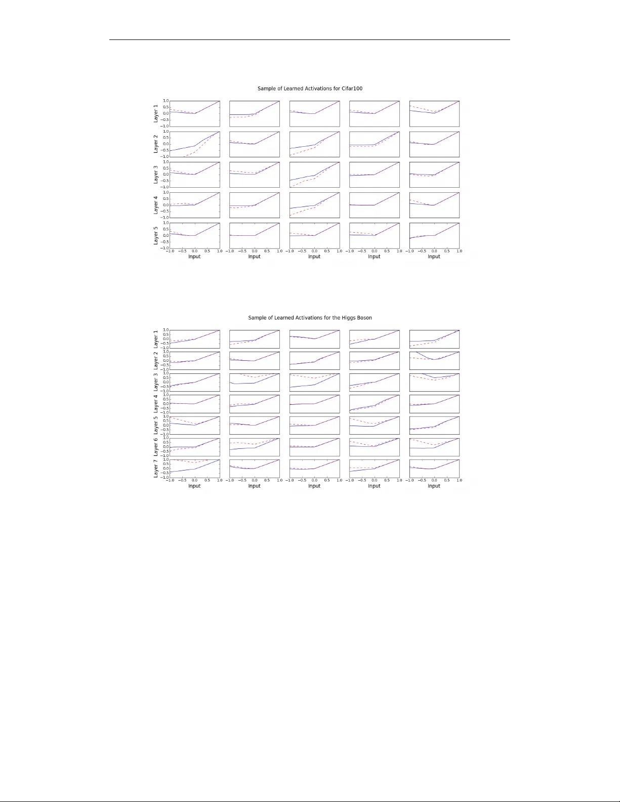
Accepted as a workshop contrib ution at ICLR 2015 L E A R N I N G A C T I V A T I O N F U N C T I O N S T O I M P RO V E D E E P N E U R A L N E T W O R K S For est Agostinelli Department of Computer Science Univ ersity of California - Irvine Irvine, CA 92697, USA { fagostin } @uci.edu Matthew Hoffman Adobe Research San Francisco, CA 94103, USA { mathoffm } @adobe.com Peter Sado wski, Pierre Baldi Department of Computer Science Univ ersity of California - Irvine Irvine, CA 92697, USA { peter.j.sadowski,pfbaldi } @uci.edu A B S T R A C T Artificial neural networks typically ha ve a fixed, non-linear activ ation function at each neuron. W e have designed a novel form of piecewise linear acti v ation func- tion that is learned independently for each neuron using gradient descent. With this adaptive activ ation function, we are able to improve upon deep neural net- work architectures composed of static rectified linear units, achie ving state-of-the- art performance on CIF AR-10 (7.51%), CIF AR-100 (30.83%), and a benchmark from high-energy physics in volving Higgs boson decay modes. 1 I N T R O D U C T I O N Deep learning with artificial neural networks has enabled rapid progress on applications in engi- neering (e.g., Krizhevsky et al., 2012; Hannun et al., 2014) and basic science (e.g., Di Lena et al., 2012; Lusci et al., 2013; Baldi et al., 2014). Usually , the parameters in the linear components are learned to fit the data, while the nonlinearities are pre-specified to be a logistic, tanh, rectified linear , or max-pooling function. A suf ficiently large neural network using any of these common nonlinear functions can approximate arbitrarily complex functions (Hornik et al., 1989; Cho & Saul, 2010), but in finite networks the choice of nonlinearity af fects both the learning dynamics (especially in deep networks) and the network’ s expressi ve po wer . Designing acti v ation functions that enable fast training of accurate deep neural networks is an acti ve area of research. The rectified linear activ ation function (Jarrett et al., 2009; Glorot et al., 2011), which does not saturate lik e sigmoidal functions, has made it easier to quickly train deep neural net- works by alle viating the difficulties of weight-initialization and v anishing gradients. Another recent innov ation is the “maxout” acti v ation function, which has achiev ed state-of-the-art performance on multiple machine learning benchmarks (Goodfello w et al., 2013). The maxout activ ation function computes the maximum of a set of linear functions, and has the property that it can approximate any con ve x function of the input. Springenberg & Riedmiller (2013) replaced the max function with a probabilistic max function and Gulcehre et al. (2014) explored an activ ation function that replaces the max function with an L P norm. Howe v er , while the type of activ ation function can have a significant impact on learning, the space of possible functions has hardly been explored. 1 Accepted as a workshop contrib ution at ICLR 2015 One way to explore this space is to learn the activ ation function during training. Previous efforts to do this hav e lar gely focused on genetic and e volutionary algorithms (Y ao, 1999), which attempt to select an activ ation function for each neuron from a pre-defined set. Recently , T urner & Miller (2014) combined this strategy with a single scaling parameter that is learned during training. In this paper , we propose a more powerful adaptiv e activ ation function. This parametrized, piecewise linear acti vation function is learned independently for each neuron using gradient descent, and can represent both con ve x and non-con ve x functions of the input. Experiments demonstrate that like other piecewise linear acti vation functions, this works well for training deep neural networks, and we obtain state-of-the-art performance on multiple benchmark deep learning tasks. 2 A D A P T I V E P I E C E W I S E L I N E A R U N I T S Here we define the adaptiv e piecewise linear (APL) acti v ation unit. Our method formulates the activ ation function h i ( x ) of an APL unit i as a sum of hinge-shaped functions, h i ( x ) = max(0 , x ) + S X s =1 a s i max(0 , − x + b s i ) (1) The result is a piece wise linear activ ation function. The number of hinges, S , is a hyperparameter set in adv ance, while the variables a s i , b s i for i ∈ 1 , ..., S are learned using standard gradient des cent during training. The a s i variables control the slopes of the linear se gments, while the b s i variables determine the locations of the hinges. The number of additional parameters that must be learned when using these APL units is 2 S M , where M is the total number of hidden units in the network. This number is small compared to the total number of weights in typical networks. Figure 1: Sample activ ation functions obtained from changing the parameters. Notice that figure b shows that the activ ation function can also be non-con ve x. Asymptotically , the activ ation func- tions tend to g ( x ) = x as x → ∞ and g ( x ) = αx − c as x ← −∞ for some α and c . S = 1 for all plots. Figure 1 shows example APL functions for S = 1 . Note that unlike maxout, the class of func- tions that can be learned by a single unit in- cludes non-con ve x functions. In fact, for large enough S , h i ( x ) can approximate arbitrarily complex continuous functions, subject to two conditions: Theorem 1 Any continuous piecewise-linear function g ( x ) can be expr essed by Equation 1 for some S , and a i , b i , i ∈ 1 , ..., S , assuming that: 1. There is a scalar u such that g ( x ) = x for all x ≥ u . 2. There ar e two scalars v and α such that ∇ x g ( x ) = α for all x < v . This theorem implies that we can reconstruct any piecewise-linear function g ( x ) over any subset of the real line, and the two conditions on g ( x ) constrain the beha vior of g ( x ) to be linear as x gets very large or small. The first condi- tion is less restricti ve than it may seem. In neu- ral networks, g ( x ) is generally only of interest as an input to a linear function wg ( x ) + z ; this linear function effecti v ely restores the two degrees of freedom that are eliminated by constraining the rightmost segment of g ( x ) to have unit slope and bias 0. Proof Let g ( x ) be piecewise linear with K + 2 linear regions separated by ordered boundary points b 0 , b 1 , ..., b K , and let a k be the slope of the k -th region. Assume also that g ( x ) = x for all x ≥ b K . 2 Accepted as a workshop contrib ution at ICLR 2015 W e show that g ( x ) can be expressed by the follo wing special case of Equation 1: h ( x ) ≡ − a 0 max(0 , − x + b 0 ) + P K k =1 a k (max(0 , − x + b k − 1 ) − max(0 , − x + b k )) − max(0 , − x ) + max(0 , x ) + max(0 , − x + b K ) , (2) The first term has slope a 0 in the range ( −∞ , b 0 ) and 0 else where. Each element in the summation term of Equation 2 has slope a k ov er the range ( b k − 1 , b k ) and 0 else where. The last three terms together have slope 1 when x ∈ ( b K , ∞ ) and 0 elsewhere. No w , g ( x ) and h ( x ) are continuous, their slopes match almost e verywhere, and it is easily verified that h ( x ) = g ( x ) = x for x ≥ b K . Thus, we conclude that h ( x ) = g ( x ) for all x .  2 . 1 C O M P A R I S O N W I T H O T H E R A C T I V A T I O N F U N C T I O N S In this section we compare the proposed approach to learning acti v ation functions with two other nonlinear activ ation functions: maxout (Goodfellow et al., 2013), and network-in-network (Lin et al., 2013). W e observ e that both maxout units and network-in-netw ork can learn any nonlinear acti v ation func- tion that APL units can, but require many more parameters to do so. This difference allows APL units to be applied in very different ways from maxout and network-in-network nonlinearities: the small number of parameters needed to tune an APL unit makes it practical to train con volutional networks that apply different nonlinearities at each point in each feature map, which would be com- pletely impractical in either maxout networks or network-in-netw ork approaches. Maxout. Maxout units differ from traditional neural network nonlinearities in that they take as input the output of multiple linear functions, and return the largest: h maxout ( x ) = max k ∈{ 1 ,...,K } w k · x + b k . (3) Incorporating multiple linear functions increases the expressiv e po wer of maxout units, allowing them to approximate arbitrary con v ex functions, and allowing the difference of a pair of maxout units to approximate arbitrary functions. Networks of maxout units with a particular weight-tying scheme can reproduce the output of an APL unit. The sum of terms in Equation 1 with positive coefficients (including the initial max(0 , x ) term) is a con ve x function, and the sum of terms with negati ve coefficients is a conca ve function. One could approximate the con v ex part with one maxout unit, and the concav e part with another maxout unit: h conv ex ( x ) = max k c conv ex k w · x + d conv ex k ; h concav e ( x ) = max k c concav e k w · x + d concav e k , (4) where c and d are chosen so that h conv ex ( x ) − h concav e ( x ) = max(0 , w · x + u ) + P s a s max(0 , w · x + u ) . (5) In a standard maxout network, howe v er , the w vectors are not tied. So implementing APL units (Equation 1) using a maxout network would require learning O ( S K ) times as many parameters, where K is the size of the maxout layer’ s input vector . Whenever the expressi ve power of an APL unit is sufficient, using the more complex maxout units is therefore a waste of computational and modeling power . Network-in-Network. Lin et al. (2013) proposed replacing the simple rectified linear activ ation in conv olutional networks with a fully connected network whose parameters are learned from data. This “MLPConv” layer couples the outputs of all filters applied to a patch, and permits arbitrarily complex transformations of the inputs. A depth- M MLPCon v layer produces an output vector f M ij from an input patch x ij via the series of transformations f 1 ij k = max(0 , w 1 k · x ij + b 1 k ) , . . . , f M ij k = max(0 , w M k · f M − 1 ij + b M k ) . (6) 3 Accepted as a workshop contrib ution at ICLR 2015 As with maxout networks, there is a weight-tying scheme that allo ws an MLPCon v layer to repro- duce the behavior of an APL unit: f 1 ij k = max(0 , c k w κ ( k ) · x ij + b 1 k ) , f 2 ij k = P ` | κ ( ` )= k a k f 1 ij ` , (7) where the function κ ( k ) maps from hinge output indices k to filter indices κ , and the coef ficient c k ∈ {− 1 , 1 } . This is a very aggressi ve weight-tying scheme that dramatically reduces the number of parameters used by the MLPCon v layer . Again we see that it is a waste of computational and modeling power to use network-in-network where v er an APL unit would suf fice. Howe v er , netw ork-in-network can do things that APL units cannot—in particular , it ef ficiently cou- ples and summarizes the outputs of multiple filters. One can get the benefits of both architectures by replacing the rectified linear units in the MLPcon v layer with APL units. 3 E X P E R I M E N T S Experiments were performed using the software package CAFFE (Jia et al., 2014). The hyperpa- rameter , S , that controls the complexity of the acti v ation function was determined using a validation set for each dataset. The a s i and b s i parameters were regularized with an L2 penalty , scaled by 0 . 001 . W ithout this penalty , the optimizer is free to choose very lar ge values of a s i balanced by very small weights, which would lead to numerical instability . W e found that adding this penalty improved re- sults. The model files and solver files are a v ailable at https://github .com/F orestAgostinelli/Learned- Activ ation-Functions-Source/tree/master . 3 . 1 C I FA R The CIF AR-10 and CIF AR-100 datasets (Krizhevsky & Hinton, 2009) are 32x32 color images that hav e 10 and 100 classes, respectively . They both have 50,000 training images and 10,000 test im- ages. The images were preprocessed by subtracting the mean v alues of each pixel of the training set from each image. Our network for CIF AR-10 was loosely based on the network used in (Sriv astav a et al., 2014). It had 3 con volutional layers with 96, 128, and 256 filters, respecti vely . Each kernel size was 5x5 and was padded by 2 pixels on each side. The con volutional layers were followed by a max-pooling, av erage-pooling, and average-pooling layer , respecti vely; all with a kernel size of 3 and a stride of 2. The two fully connected layers had 2048 units each. W e applied dropout (Hinton et al., 2012) to the network as well. W e found that applying dropout both before and after a pooling layer increased classification accuracy . The probability of a unit being dropped before a pooling layer was 0.25 for all pooling layers. The probability for them being dropped after each pooling layers was 0.25, 0.25, and 0.5, respecti vely . The probability of a unit being dropped for the fully connected layers was 0.5 for both layers. The final layer was a softmax classification layer . For CIF AR-100, the only dif ference was the second pooling layer was max-pooling instead of av erage-pooling. The baseline used rectified linear activ ation functions. When using the APL units, for CIF AR-10, we set S = 5 . For CIF AR-100 we set S = 2 . T able 1 shows that adding the APL units improved the baseline by ov er 1% in the case of CIF AR-10 and by almost 3% in the case of CIF AR-100. In terms of r elative differ ence, this is a 9.4% and a 7.5% decr ease in err or rate, r espectively . W e also try the network-in-network architecture for CIF AR-10 (Lin et al., 2013). W e ha ve S = 2 for CIF AR-10 and S = 1 for CIF AR-100. W e see that it improves performance for both datasets. W e also try our method with the augmented version of CIF AR-10 and CIF AR-100. W e pad the image all around with a four pixel border of zeros. For training, we take random 32 x 32 crops of the image and randomly do horizontal flips. For testing we just take the center 32 x 32 image. T o the best of our kno wledge, the results we report for data augmentation using the network-in-netw ork architecture ar e the best r esults r eported for CIF AR-10 and CIF AR-100 for any method. In section 3.4, one can observe that the learned acti vations can look similar to leak y rectified linear units (Leaky ReLU) (Maas et al., 2013). This activ ation function is slightly different than the ReLU 4 Accepted as a workshop contrib ution at ICLR 2015 because it has a small slope k when the input x < 0 . h ( x ) =  x, if x > 0 k x, otherwise In (Maas et al., 2013), k is equal to 0 . 01 . T o compare Leaky ReLUs to our method, we try different values for k and pick the best value one. The possible values are positi ve and negati v e 0 . 01 , 0 . 05 , 0 . 1 , and 0 . 2 . For the standard conv olutional neural network architecture k = 0 . 05 for CIF AR-10 and k = − 0 . 05 for CIF AR-100. For the network-in-network architecture k = 0 . 05 for CIF AR-10 and k = 0 . 2 for CIF AR-100. APL units consistently outperform leaky ReLU units, showing the value of tuning the nonlinearity (see also section 3.3). T able 1: Error rates on CIF AR-10 and CIF AR-100 with and without data augmentation. This in- cludes standard con v olutional neural netw orks (CNNs) and the network-in-netw ork (NIN) architec- ture (Lin et al., 2013). The networks were trained 5 times using different random initializations — we report the mean followed by the standard de viation in parenthesis. The best results are in bold. Method CIF AR-10 CIF AR-100 W ithout Data Augmentation CNN + ReLU (Sriv asta v a et al., 2014) 12.61% 37.20% CNN + Channel-Out (W ang & JaJa, 2013) 13.2% 36.59% CNN + Maxout (Goodfellow et al., 2013) 11.68% 38.57% CNN + Probout (Springenberg & Riedmiller, 2013) 11.35% 38.14% CNN (Ours) + ReLU 12.56 (0.26)% 37.34 (0.28)% CNN (Ours) + Leaky ReLU 11.86 (0.04)% 35.82 (0.34)% CNN (Ours) + APL units 11.38 (0.09)% 34.54 (0.19)% NIN + ReLU (Lin et al., 2013) 10.41% 35.68% NIN + ReLU + Deep Supervision (Lee et al., 2014) 9.78% 34.57% NIN (Ours) + ReLU 9.67 (0.11)% 35.96 (0.13)% NIN (Ours) + Leaky ReLU 9.75 (0.22)% 36.00 (0.36)% NIN (Ours) + APL units 9.59 (0.24)% 34.40 (0.16)% W ith Data Augmentation CNN + Maxout (Goodfellow et al., 2013) 9.38% - CNN + Probout (Springenberg & Riedmiller, 2013) 9.39% - CNN + Maxout (Stollenga et al., 2014) 9.61% 34.54% CNN + Maxout + Selectiv e Attention (Stollenga et al., 2014) 9.22% 33.78% CNN (Ours) + ReLU 9.99 (0.09)% 34.50 (0.12)% CNN (Ours) + APL units 9.89 (0.19)% 33.88 (0.45)% NIN + ReLU (Lin et al., 2013) 8.81% - NIN + ReLU + Deep Supervision (Lee et al., 2014) 8.22% - NIN (Ours) + ReLU 7.73 (0.13)% 32.75 (0.13)% NIN (Ours) + APL units 7.51 (0.14)% 30.83 (0.24)% 3 . 2 H I G G S B O S O N D E C A Y The Higgs-to- τ + τ − decay dataset comes from the field of high-energy physics and the analysis of data generated by the Large Hadron Collider (Baldi et al., 2015). The dataset contains 80 million collision ev ents, characterized by 25 real-valued features describing the 3D momenta and energies of the collision products. The supervised learning task is to distinguish between two types of physical processes: one in which a Higgs boson decays into τ + τ − leptons and a background process that produces a similar measurement distribution. Performance is measured in terms of the area under the receiv er operating characteristic curve (A UC) on a test set of 10 million examples, and in terms of discovery significance (Cow an et al., 2011) in units of Gaussian σ , using 100 signal events and 5000 background ev ents with a 5% relati ve uncertainty . Our baseline for this experiment is the 8 layer neural network architecture from (Baldi et al., 2015) whose architecture and training hyperparameters were optimized using the Spearmint al- gorithm (Snoek et al., 2012). W e used the same architecture and training parameters except that 5 Accepted as a workshop contrib ution at ICLR 2015 dropout was used in the top two hidden layers to reduce overfitting. For the APL units we used S = 2 . T able 2 sho ws that a single network with APL units achiev es state-of-the-art performance, increasing performance over the dropout-trained baseline and the ensemble of 5 neural networks from (Baldi et al., 2015). T able 2: Performance on the Higgs boson decay dataset in terms of both A UC and expected dis- cov ery significance. The networks were trained 4 times using dif ferent random initializations — we report the mean followed by the standard de viation in parenthesis. The best results are in bold. Method A UC Discovery Significance DNN + ReLU (Baldi et al., 2015) 0.802 3.37 σ DNN + ReLU + Ensemble(Baldi et al., 2015) 0.803 3.39 σ DNN (Ours) + ReLU 0.803 (0.0001) 3.38 (0.008) σ DNN (Ours) + APL units 0.804 (0.0002) 3.41 (0.006) σ 3 . 3 E FF E C T S O F A P L U N I T H Y P E R PA R A M E T E R S T able 3 shows the ef fect of v arying S on the CIF AR-10 benchmark. W e also tested whether learning the activ ation function was important (as opposed to having complicated, fixed acti v ation functions). For S = 1 , we tried freezing the acti v ation functions at their random initialized positions, and not allowing them to learn. The results show that learning activ ations, as opposed to keeping them fix ed, results in better performance. T able 3: Classification accuracy on CIF AR-10 for v arying values of S . Shown are the mean and standard deviation o ver 5 trials. V alues of S Error Rate baseline 12.56 (0.26)% S = 1 (activ ation not learned) 12.55 (0.11)% S = 1 11.59 (0.16)% S = 2 11.73 (0.23)% S = 5 11.38 (0.09)% S = 10 11.60 (0.16)% 3 . 4 V I S UA L I Z A T I O N A N D A NA L Y S I S O F A D A P T I V E P I E C E W I S E L I N E A R F U N C T I O N S The div ersity of adapti ve piecewise linear functions was visualized by plotting h i ( x ) for sample neurons. Figures 2 and 3 show adapti ve piece wise linear functions for the CIF AR-100 and Higgs → τ + τ − experiments, along with the random initialization of that function. In figure 4, for each layer, 1000 acti v ation functions (or the maximum number of activ ation functions for that layer, whichev er is smaller) are plotted. One can see that there is greater variance in the learned activ ations for CIF AR-100 than there is for CIF AR-10. There is greater variance in the learned acti v ations for Higgs → τ + τ − than there is for CIF AR-100. For the case of Higgs → τ + τ − , a trend that can be seen is that the variance decreases in the higher layers. 4 C O N C L U S I O N W e hav e introduced a novel neural network activ ation function in which each neuron computes an independent, piece wise linear function. The parameters of each neuron-specific activ ation function are learned via gradient descent along with the network’ s weight parameters. Our experiments demonstrate that learning the acti vation functions in this way can lead to significant performance improv ements in deep neural networks without significantly increasing the number of parameters. Furthermore, the networks learn a di verse set of acti vation functions, suggesting that the standard one-activ ation-function-fits-all approach may be suboptimal. 6 Accepted as a workshop contrib ution at ICLR 2015 Figure 2: CIF AR-100 Sample Acti v ation Functions. Initialization (dashed line) and the final learned function (solid line). Figure 3: Higgs → τ + τ − Sample Activ ation Functions. Initialization (dashed line) and the final learned function (solid line). A C K N OW L E D G M E N T S F . Agostinelli was supported by the GEM Fellowship. This work was done during an internship at Adobe. W e also wish to acknowledge the support of NVIDIA Corporation with the donation of the T esla K40 GPU used for this research, NSF grant IIS-0513376, and a Google Faculty Research award to P . Baldi, and thanks to Y uzo Kanomata for computing support. R E F E R E N C E S Baldi, P , Sadowski, P , and Whiteson, D. Searching for exotic particles in high-energy physics with deep learning. Natur e Communications , 5, 2014. Baldi, Pierre, Sadowski, Peter , and Whiteson, Daniel. Enhanced higgs to τ + τ − searches with deep learning. Physics Revie w Letters , 2015. In press. Cho, Y oungmin and Saul, La wrence. Large mar gin classification in infinite neural networks. Neural Computation , 22(10), 2010. 7 Accepted as a workshop contrib ution at ICLR 2015 (a) CIF AR-10 Activ ation Functions. (b) CIF AR-100 Activ ation Functions. (c) Higgs → τ + τ − Activ ation Functions. Figure 4: V isualization of the range of the values for the learned activ ation functions for the deep neural network for the CIF AR datasets and Higgs → τ + τ − dataset. Cow an, Glen, Cranmer, K yle, Gross, Eilam, and V itells, Ofer . Asymptotic formulae for likelihood- based tests of ne w ph ysics. Eur .Phys.J. , C71:1554, 2011. doi: 10.1140/epjc/s10052- 011- 1554- 0. Di Lena, P ., Nagata, K., and Baldi, P . Deep architectures for protein contact map prediction. Bioin- formatics , 28:2449–2457, 2012. doi: 10.1093/bioinformatics/bts475. First published online: July 30, 2012. Glorot, Xavier , Bordes, Antoine, and Bengio, Y oshua. Deep sparse rectifier networks. In Pr oceed- ings of the 14th International Conference on Artificial Intelligence and Statistics. JMLR W&CP V olume , volume 15, pp. 315–323, 2011. Goodfellow , Ian J, W arde-Farley , Da vid, Mirza, Mehdi, Courville, Aaron, and Bengio, Y oshua. Maxout networks. arXiv preprint , 2013. Gulcehre, Caglar , Cho, Kyunghyun, Pascanu, Razvan, and Bengio, Y oshua. Learned-norm pool- ing for deep feedforward and recurrent neural networks. In Machine Learning and Knowledge Discovery in Databases , pp. 530–546. Springer , 2014. Hannun, A wni Y ., Case, Carl, Casper , Jared, Catanzaro, Bryan C., Diamos, Greg, Elsen, Erich, Prenger , Ryan, Satheesh, Sanjee v , Sengupta, Shubho, Coates, Adam, and Ng, Andrew Y . Deep 8 Accepted as a workshop contrib ution at ICLR 2015 speech: Scaling up end-to-end speech recognition. CoRR , abs/1412.5567, 2014. URL http: //arxiv.org/abs/1412.5567 . Hinton, Geoffre y E, Sriv astav a, Nitish, Krizhevsky , Ale x, Sutske ver , Ilya, and Salakhutdinov , Rus- lan R. Improving neural networks by pre v enting co-adaptation of feature detectors. arXiv pr eprint arXiv:1207.0580 , 2012. Hornik, Kurt, Stinchcombe, Maxwell, and White, Halbert. Multilayer feedforward networks are univ ersal approximators. Neural networks , 2(5):359–366, 1989. Jarrett, K e vin, Ka vukcuoglu, K oray , Ranzato, M, and LeCun, Y ann. What is the best multi-stage ar- chitecture for object recognition? In Computer V ision, 2009 IEEE 12th International Conference on , pp. 2146–2153. IEEE, 2009. Jia, Y angqing, Shelhamer , Evan, Donahue, Jeff, Karayev , Serge y , Long, Jonathan, Girshick, Ross, Guadarrama, Sergio, and Darrell, T re vor . Caffe: Con v olutional architecture for fast feature em- bedding. arXiv pr eprint arXiv:1408.5093 , 2014. Krizhevsk y , Alex and Hinton, Geoffre y . Learning multiple layers of features from tiny images. Computer Science Department, University of T or onto, T ech. Rep , 2009. Krizhevsk y , Ale x, Sutskev er , Ilya, and Hinton, Geof frey E. Imagenet classification with deep con v o- lutional neural networks. In Advances in neural information pr ocessing systems , pp. 1097–1105, 2012. Lee, Chen-Y u, Xie, Saining, Gallagher , Patrick, Zhang, Zhengyou, and Tu, Zhuo wen. Deeply- supervised nets. arXiv pr eprint arXiv:1409.5185 , 2014. Lin, Min, Chen, Qiang, and Y an, Shuicheng. Network in network. arXiv pr eprint arXiv:1312.4400 , 2013. Lusci, Alessandro, Pollastri, Gianluca, and Baldi, Pierre. Deep architectures and deep learning in chemoinformatics: the prediction of aqueous solubility for drug-like molecules. Journal of chemical information and modeling , 53(7):1563–1575, 2013. Maas, Andrew L, Hannun, A wni Y , and Ng, Andrew Y . Rectifier nonlinearities improve neural network acoustic models. In Proc. ICML , v olume 30, 2013. Snoek, Jasper , Larochelle, Hugo, and Adams, Ryan P . Practical bayesian optimization of machine learning algorithms. In Advances in Neural Information Pr ocessing Systems , pp. 2951–2959, 2012. Springenberg, Jost T obias and Riedmiller, Martin. Improving deep neural networks with probabilis- tic maxout units. arXiv pr eprint arXiv:1312.6116 , 2013. Sriv asta v a, Nitish, Hinton, Geoffrey , Krizhevsk y , Ale x, Sutskev er , Ilya, and Salakhutdinov , Ruslan. Dropout: A simple way to prev ent neural networks from overfitting. The J ournal of Machine Learning Resear ch , 15(1):1929–1958, 2014. Stollenga, Marijn F , Masci, Jonathan, Gomez, Faustino, and Schmidhuber , J ¨ urgen. Deep networks with internal selective attention through feedback connections. In Advances in Neural Information Pr ocessing Systems , pp. 3545–3553, 2014. T urner , Andrew James and Miller , Julian Francis. Neuroev olution: Evolving heterogeneous artificial neural networks. Evolutionary Intelligence , pp. 1–20, 2014. W ang, Qi and JaJa, Joseph. From maxout to channel-out: Encoding information on sparse pathways. arXiv pr eprint arXiv:1312.1909 , 2013. Y ao, Xin. Evolving artificial neural networks. Pr oceedings of the IEEE , 87(9):1423–1447, 1999. 9