A Singular Value Decomposition-based Factorization and Parsimonious Component Model of Demographic Quantities Correlated by Age: Predicting Complete Demographic Age Schedules with Few Parameters

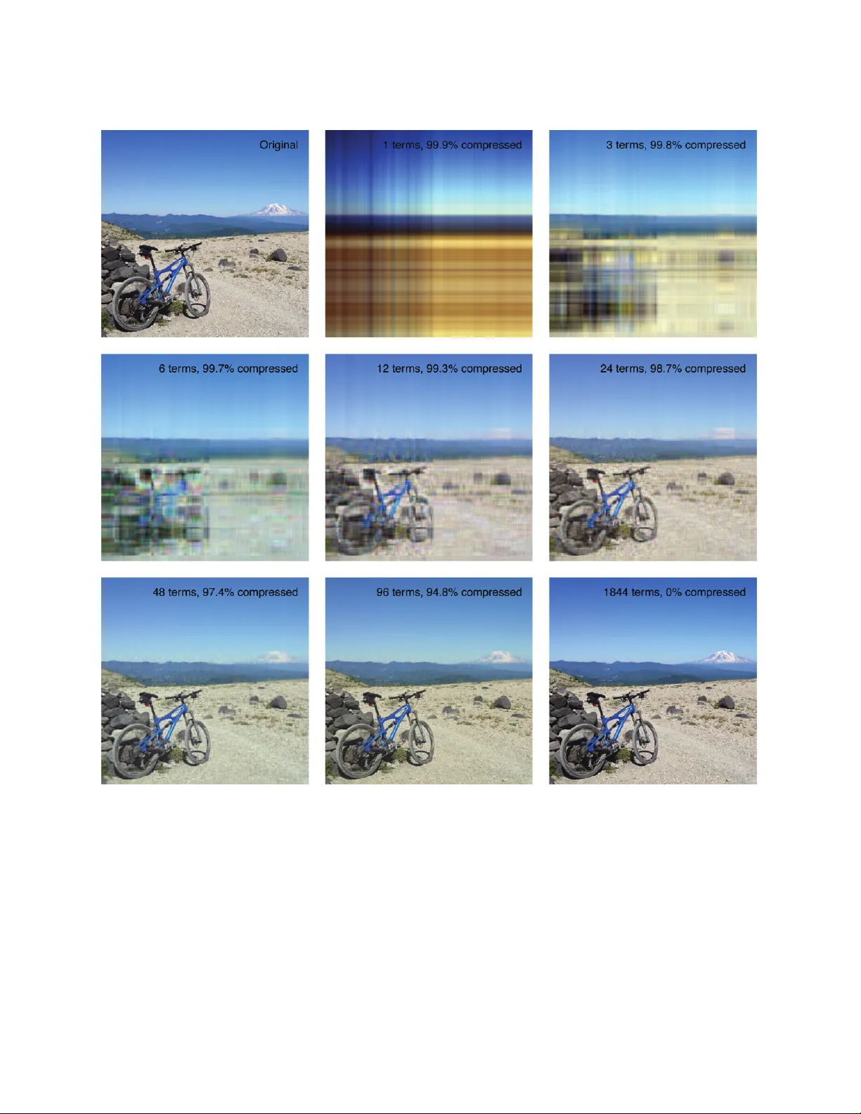
A Singular V alue Decomposition-based F a ctoriza tion and P arsimonious Component Model of Demographic Quantities Correla ted by A ge Predicting Complete Demographic A ge Schedules with Few P arameters Sam uel J. Clark 1,2,3,4,* 1 Departmen t of Sociology , Univ ersit y of W ashington 2 MR C/Wits Rural Public Health and Health T ransitions Researc h Unit (Agincourt), Sc ho ol of Public Health, F aculty of Health Sciences, Univ ersit y of the Witw atersrand 3 ALPHA Netw ork, London School of Hygience and T ropical Medicine, London, UK 4 INDEPTH Net w ork, Accra, Ghana * Corresp ondence to: work@samclark.net Ma y 8, 2014 i Abstract Bac kground. F ormal demography has a long history of building simple models of age schedules of demographic quantities, e.g. mortalit y and fertility rates. These are widely used in demographic metho ds to manipulate whole age schedules using few parameters. Ob jectiv e. The Singular V alue Decomp osition (SVD) factorizes a matrix into three matrices with useful properties including the abilit y to reconstruct the original matrix using many few er, simple matrices. This work demonstrates ho w these prop erties can b e exploited to build parsimonious mo dels of whole age schedules of demographic quan tities that can b e further parameterized in terms of arbitrary co v ariates. Metho ds. The SVD is presented and explained in detail with attention to developing an intuitiv e understanding. The SVD is used to construct a general, comp onen t mo del of demographic age sc hedules, and that model is demonstrated with age-speciﬁc mortality and fertility rates. Finally , the mo del is used (1) to predict age-sp eciﬁc mortality using HIV indicators and summary mea- sures of age-speciﬁc mortality , and (2) to predict age-speciﬁc fertility using the total fertility rate (TFR). Results. The component model of age-speciﬁc mortalit y and fertilit y rates succeeds in reproducing the data with tw o inputs, and acting through those tw o inputs, v arious cov ariates are able to accurately predict full age schedules. Conclusions. The SVD is a p oten tially useful as a w ay to summarize, smo oth and mo del age- sp eciﬁc demographic quan tities. The comp onen t mo del is a general method of relating co v ariates to whole age sc hedules. Commen ts. The focus of this w ork is the SVD and the comp onen t model. The applications are for illustrative purp oses only . Keywor ds: Singular V alue Decomposition, SVD, Age-sp eciﬁc Mo del, Comp onent Model, Mortality , F ertility , Predicting demographic age sc hedules. A cknowledgments This w ork was supp orted by grants K01 HD057246 and R01 HD054511 and from the Eunice Kennedy Shriver National Institute of Child Health and Human Developmen t (NICHD). The fun- ders had no role in study design, data collection and analysis, decision to publish, or preparation of the manuscript. The work describ ed b elow w as conducted in the R programming language and run in the R statistical soft ware pack age (R F oundation for Statistical Computing, 2014). Da vid Shar- ro w and Adrian Raftery ha ve b een colleagues working on related topics for some time, and their advice and feedbac k were imp ortant to writing this pap er. Jon W ak eﬁeld and Tyler McCormick read drafts of this article and provided helpful commen ts. ii Con ten ts 1 In tro duction 1 2 The Singular V alue Decomp osition 2 2.1 Sk etch of a Linear Algebra Deriv ation of the SVD . . . . . . . . . . . . . . . . . . . 2 2.2 The Singular V alue Decomposition and Principal Component Analysis . . . . . . . . 2 3 Matrix Approximation and a useful Geometric Interpretation of the SVD 3 3.1 The SVD as a Sum of Rank-1 Matrices . . . . . . . . . . . . . . . . . . . . . . . . . . 3 3.2 Eac h Column of the Data Matrix as a Sum of Left Singular V ectors . . . . . . . . . 6 3.3 A P arsimonious Mo del and Smoother for V ectors Similar to the Columns of the Data Matrix . . . . . . . . . . . . . . . . . . . . . . . . . . . . . . . . . . . . . . . . . . . . 8 3.4 A Simple 3 × 2 Example SVD with Geometric In terpretation . . . . . . . . . . . . . 8 4 The SVD and Demographic Quantities Correlated by Age 14 4.1 Demographic Quantities Correlated by Age – A ge Sche dules . . . . . . . . . . . . . . 14 4.2 A General, Parsimonious, SVD-derived Mo del for Demographic Quantities Corre- lated by Age . . . . . . . . . . . . . . . . . . . . . . . . . . . . . . . . . . . . . . . . 15 4.2.1 Data and Model Ob jectives . . . . . . . . . . . . . . . . . . . . . . . . . . . . 18 4.2.2 The Mo del – Summarizing Empirical Regularities . . . . . . . . . . . . . . . . 18 4.2.3 P arameters as F unctions of Co v ariates – Predicting Age Sc hedules . . . . . . 22 4.2.4 Iden tifying Clusters in Collections of Empirical Age Schedules . . . . . . . . . 22 5 Examples 22 5.1 Example Data: The Agincourt HDSS, South Africa . . . . . . . . . . . . . . . . . . . 22 5.2 Comp onen t Mo del for Mortality . . . . . . . . . . . . . . . . . . . . . . . . . . . . . 23 5.2.1 Mortalit y Age Schedule Cov ariates and Predictors . . . . . . . . . . . . . . . 24 5.2.2 Iden tifying ‘Common’ Age Sc hedules of Mortality . . . . . . . . . . . . . . . . 29 5.3 Comp onen t Mo del for F ertilit y . . . . . . . . . . . . . . . . . . . . . . . . . . . . . . 30 5.3.1 F ertility Age Sc hedule Co v ariates and Predictors . . . . . . . . . . . . . . . . 32 6 Discussion 33 App endices 38 A Example Data 38 B Smo othed Agincourt Mortality Rates 39 C Smo othed Agincourt F ertility Rates 41 D Predicted Age-Sp eciﬁc Mortality Plots 42 E Predicted Age-Sp eciﬁc F ertility Plots 62 iii 1 In tro duction A long-standing pursuit of formal demography is the construction of empirical mo dels of quantities that v ary predictably by age (Coale and T russell, 1996). Model life tables (e.g. Coale and Demeny, 1966; United Nations. Departmen t of In ternational Economic and So cial Aﬀairs, 1982; Murray et al., 2003; W ang et al., 2013) and v arious mortalit y models (e.g. Wilmoth et al., 2012; Heligman and Pollard, 1980) aim to iden tify and parsimoniously express the regularit y of mortality with age, and some fertilit y mo dels (e.g. Coale and T russell, 1974) do the same. Because age is a strong predictor of these quan tities, age proﬁles of these quantities from diﬀerent p opulations, times and places are correlated. This fact allows us to tak e adv an tage of the singular v alue decomp osition (SVD), a classic and long-standing result in mathematics (Stew art, 1993), to construct a general, parsimonious, weigh ted sum-based mo del of the age pattern of demographic quan tities that can incorp orate cov ariates and b e used to make predictions. The SVD has b een used b efore in demography . Building on earlier work by Wilmoth et al. (1989), Lee and Carter (1992) use the SVD to generate a rank-1 approximation of the residual produced b y subtracting the mean from a matrix of log mortalit y rates, eﬀectively yielding a least-squares solution for an under-determined part of their mo del (Wilmoth, 1993; Go o d, 1969, and Section 3.1, Equation 8). This is similar in spirit to what we develop b elow but solv es a diﬀeren t, sp eciﬁc problem and do es not iden tify or develop the generalizable features of the SVD of age-correlated quan tities or in a general sense exploit the properties of the reduced-rank form of the SVD. Later Wilmoth et al. (2012) again use the SVD in a similar wa y to characterize the age-pattern of residuals in the their Log-Quad mo del. In earlier work (Clark et al., 2009; INDEPTH Net work [Prepared by Sam uel J. Clark], 2002; Clark, 2001; Sharro w et al., 2014) w e hav e developed and used a precursor of the weigh ted sum, component model that w e fully dev elop b elo w, and in the most recen t iteration w e use the SVD to construct the comp onen ts - without fully exploiting its capabilities. Finally , F osdick and Hoﬀ (2012) dev elop a separable co v ariance mo del and demonstrate it using age-speciﬁc mortalit y . This w ork fo cuses on the co v ariance model of the mean-subtracted mortalit y rates and lik e the others do es not identify or develop the general implications of the generic SVD for age- correlated quantities. The purp ose of this work is to discuss the SVD in detail and demonstrate how it can b e used to dev elop a general, parsimonious mo del of demographic quantities correlated b y age. The intended audience is demographers who might w an t to use the mo del. With that in mind the presentation is in tuitive with an emphasis on geometric in terpretations rather than mathematically rigorous, and it is supp orted by sev eral fully work ed examples. There are many mathematical presentations of the SVD elsewhere, e.g. Go o d (1969); Kalman (1996); Strang (2009). The remainder of the article b egins with a detailed presentation of what the SVD is and how it is related to principal comp onents analysis (PCA). That is follow ed b y a re-expression of the SVD of a data matrix X in a form that expresses each column v ector of X as a weigh ted sum of increasingly less consequential terms. That result is used to dev elop a general, parsimonious mo del of demographic age proﬁles, and ﬁnally , that mo del is explored and demonstrated thoroughly using mortalit y and fertilit y data from the Agincourt health and demographic surveillance system (HDSS) in South Africa (Kahn et al., 2012). 1 2 The Singular V alue Decomp osition This section presents the SVD drawing on Strang’s presentation (Strang, 2009) and can b e skipp ed b y those who do not wan t to kno w the origin of the SVD or ho w it relates to PCA. 2.1 Sk etc h of a Linear Algebra Deriv ation of the SVD Imagine an arbitrary m × n linear transformation (or data matrix) X . The ro w-space of X con tains v ectors with n elements in R n , and the column-space vectors with m elements in R m . The SVD results from the identiﬁcation of an orthonormal basis V in the row-space of X that when trans- formed b y X yields another orthonormal basis U in the column-space of X , p otentially stretc hed b y a diagonal matrix with p ositive en tries S , XV = US , (1) X = USV − 1 , and b ecause V is orthogonal, X = USV T . (2) Equation 2 is the SVD of X . The column v ectors of U are the ‘left singular vectors’, the col- umn vectors of V are the singular vectors, and S is a diagonal matrix containing the ‘singular v alues’. 2.2 The Singular V alue Decomposition and Principal Comp onen t Analysis The natural question no w is how to identify U , V , and S . Beginning with U , we examine the SVD of X T X . X T X is sp ecial because it is p ositiv e and semi-deﬁnite, all of which means it has a w ell- b eha v ed eigen decomp osition with real, pairwise orthogonal eigen v ectors (when their eigenv alues are diﬀerent) and positive or null eigenv alues. Using Equation 2 and the fact that U T U is the iden tity matrix (because U is orthogonal), X T X = ( VSU T )( USV T ) , = VS 2 V T . (3) The righ t-hand side of Equation 3 is the eigen decomp osition of X T X which means that V con tains the eigen vectors of X T X and the elements of S 2 are the eigenv alues of X T X . W e can iden tify U in a similar w ay b y examining the SVD of XX T , which is again positive and semi-deﬁnite, XX T = ( USV T )( VSU T ) , = US 2 U T . (4) Equation 4 says that U contains the eigen vectors of XX T , and again the elemen ts of S 2 are the eigen v alues of XX T , the same as the eigen v alues of X T X . T ogether Equations 3 and 4 give us a w ay to iden tify all the components of the SVD 1 . 1 In practice this is not how the SVD is calculated; it is generally numerically easier and less uncertain to calculate the SVD directly (Kalman, 1996) and use the SVD to calculate eigen decomp ositions. 2 Those same equations explain how the SVD is related PCA. PCA is typically conducted by taking the eigen decomp osition of either the co v ariance or correlation matrix. In b oth cases the ﬁrst eigen vector lines up with the axis along whic h there is most v ariation in the cloud of data points, and subsequen t eigenv ectors p oin t in orthogonal directions and capture in decreasing quan tities the remaining v ariation in the data cloud, see Ab di and Williams (2010). Both the SVD and PCA identify the same dominan t dimensions in prepro cessed v ersions of the data matrix X (Ab di and Williams, 2010; W all et al., 2003). Both the co v ariance and correlation matrices can be calculated as X T ∗ X ∗ where X ∗ is a preprocessed v ersion of X . The co v ariance matrix is X T ms X ms , a cen tered and scaled version of X T X , computed from X ms (mean subtracted) which is created by subtracting the column mean from each column of X and m ultiplying each elemen t of the result by either 1 √ N or 1 √ N − 1 . The correlation matrix is formed by additional pro cessing of the v ariables. In addition to centering and scaling b y 1 √ N − 1 , each v ariable is normalized (to accoun t for diﬀeren t scales) by dividing by its norm, the square ro ot of the sum of its squared elemen ts, to form X msn (mean subtracted, normalized). The correlation matrix is then X T msn X msn . The eigenv ectors of the co v ariance matrix are the right singular vectors V of the SVD of X ms , and the eigenv ectors of the correlation matrix are the righ t singular vectors of the SVD of X msn . In b oth cases the singular v alues are the square ro ots of the eigen v alues. Both the cov ariance and correlation matrices are eﬀectively centered and scaled v ersions of the original data, and hence b oth the SVD of X ∗ and the eigen decomp osition of X T ∗ X ∗ yield primary dimensions of the cen tered data cloud, and b ecause the cloud is centered, these primary dimensions will line up with the orthogonal dimensions of greatest v ariation in the cloud. As we saw ab o v e in Equation 3 the SVD of X and the eigen decomp osition of X T X identify the same primary dimensions, but these will not necessarily line up with the dimensions of greatest v ariation in the cloud of data p oin ts b ecause the ﬁrst primary dimension simply p oints from the origin to the data cloud. Consequently , the ﬁrst primary dimension will corresp ond to the dimension of maxim um v ariation in the cloud only if that dimension happ ens to lie on the line from the origin to the center of the cloud. The characteristics of the SVD and PCA are display ed graphically in Figure 1. 3 Matrix A ppro ximation and a useful Geometric Interpretation of the SVD F or our purp oses there is another equiv alen t and more useful wa y of understanding the SVD as a sum of rank-1 matrices that can b e rearranged to express eac h column of X as a w eighted sum of the column v ectors of U . Below w e deriv e this re-expression and then discuss wh y it is useful. 3.1 The SVD as a Sum of Rank-1 Matrices Let the data matrix X b e an arbitrary K × L matrix or real v alues with rank( X ) = ρ ; ρ ≤ min( K, L ). The rank of a matrix is the num b er of indep endent ro ws and columns that it has; the n umber of columns and rows that cannot be expressed as m ultiplies of others. In tuitiv ely this is the n umber of dimensions deﬁned or actually o ccupied by the column and ro w v ectors in the matrix. Now, let the factors of the SVD be: • U , a K × ρ matrix whose column vectors are the left singular vectors. 3 A B ● ● ● ● ● ● ● ● ● ● ● ● ● ● ● ● ● ● ● ● ● ● ● ● ● ● ● ● ● ● ● ● ● ● ● ● ● ● ● ● ● ● ● ● ● ● ● ● ● ● ● ● ● ● ● ● ● ● ● ● ● ● ● ● ● ● ● ● ● ● ● ● ● ● ● ● ● ● ● ● ● ● ● ● ● ● ● ● ● ● ● ● ● ● ● ● ● ● ● ● ● ● ● ● ● ● ● ● ● ● ● ● ● ● ● ● ● ● ● ● ● ● ● ● ● ● ● ● ● ● ● ● ● ● ● ● ● ● ● ● ● ● ● ● ● ● ● ● ● ● ● ● ● ● ● ● ● ● ● ● ● ● ● ● ● ● ● ● ● ● ● ● ● ● ● ● ● ● ● ● ● ● ● ● ● ● ● ● ● ● ● ● ● ● ● ● ● ● ● ● −50 0 50 100 150 200 250 −50 0 50 100 150 200 250 X 1 X 2 ● ● ● ● ● ● ● ● ● ● ● ● ● ● ● ● ● ● ● ● ● ● ● ● ● ● ● ● ● ● ● ● ● ● ● ● ● ● ● ● ● ● ● ● ● ● ● ● ● ● ● ● ● ● ● ● ● ● ● ● ● ● ● ● ● ● ● ● ● ● ● ● ● ● ● ● ● ● ● ● ● ● ● ● ● ● ● ● ● ● ● ● ● ● ● ● ● ● ● ● ● ● ● ● ● ● ● ● ● ● ● ● ● ● ● ● ● ● ● ● ● ● ● ● ● ● ● ● ● ● ● ● ● ● ● ● ● ● ● ● ● ● ● ● ● ● ● ● ● ● ● ● ● ● ● ● ● ● ● ● ● ● ● ● ● ● ● ● ● ● ● ● ● ● ● ● ● ● ● ● ● ● ● ● ● ● ● ● ● ● ● ● ● ● ● ● ● ● ● ● −50 0 50 100 150 200 250 −50 0 50 100 150 200 250 X 1 X 2 C D ● ● ● ● ● ● ● ● ● ● ● ● ● ● ● ● ● ● ● ● ● ● ● ● ● ● ● ● ● ● ● ● ● ● ● ● ● ● ● ● ● ● ● ● ● ● ● ● ● ● ● ● ● ● ● ● ● ● ● ● ● ● ● ● ● ● ● ● ● ● ● ● ● ● ● ● ● ● ● ● ● ● ● ● ● ● ● ● ● ● ● ● ● ● ● ● ● ● ● ● ● ● ● ● ● ● ● ● ● ● ● ● ● ● ● ● ● ● ● ● ● ● ● ● ● ● ● ● ● ● ● ● ● ● ● ● ● ● ● ● ● ● ● ● ● ● ● ● ● ● ● ● ● ● ● ● ● ● ● ● ● ● ● ● ● ● ● ● ● ● ● ● ● ● ● ● ● ● ● ● ● ● ● ● ● ● ● ● ● ● ● ● ● ● ● ● ● ● ● ● −50 0 50 100 150 200 250 −50 0 50 100 150 200 250 X 1 X 2 ● ● ● ● ● ● ● ● ● ● ● ● ● ● ● ● ● ● ● ● ● ● ● ● ● ● ● ● ● ● ● ● ● ● ● ● ● ● ● ● ● ● ● ● ● ● ● ● ● ● ● ● ● ● ● ● ● ● ● ● ● ● ● ● ● ● ● ● ● ● ● ● ● ● ● ● ● ● ● ● ● ● ● ● ● ● ● ● ● ● ● ● ● ● ● ● ● ● ● ● ● ● ● ● ● ● ● ● ● ● ● ● ● ● ● ● ● ● ● ● ● ● ● ● ● ● ● ● ● ● ● ● ● ● ● ● ● ● ● ● ● ● ● ● ● ● ● ● ● ● ● ● ● ● ● ● ● ● ● ● ● ● ● ● ● ● ● ● ● ● ● ● ● ● ● ● ● ● ● ● ● ● ● ● ● ● ● ● ● ● ● ● ● ● ● ● ● ● ● ● ● ● ● ● ● ● ● ● ● ● ● ● ● ● ● ● ● ● ● ● ● ● ● ● ● ● ● ● ● ● ● ● ● ● ● ● ● ● ● ● ● ● ● ● ● ● ● ● ● ● ● ● ● ● ● ● ● ● ● ● ● ● ● ● ● ● ● ● ● ● ● ● ● ● ● ● ● ● ● ● ● ● ● ● ● ● ● ● ● ● ● ● ● ● ● ● ● ● ● ● ● ● ● ● ● ● ● ● ● ● ● ● ● ● ● ● ● ● ● ● ● ● ● ● ● ● ● ● ● ● ● ● ● ● ● ● ● ● ● ● ● ● ● ● ● ● ● ● ● ● ● ● ● ● ● ● ● ● ● ● ● ● ● ● ● ● ● ● ● ● ● ● ● ● ● ● ● ● ● ● ● ● ● ● ● ● ● ● ● ● ● ● ● ● ● ● ● ● ● ● −50 0 50 100 150 200 250 −50 0 50 100 150 200 250 X 1 X 2 ● ● ● ● ● ● ● ● ● ● ● ● ● ● ● ● ● ● ● ● ● ● ● ● ● ● ● ● ● ● ● ● ● ● ● ● ● ● ● ● ● ● ● ● ● ● ● ● ● ● ● ● ● ● ● ● ● ● ● ● ● ● ● ● ● ● ● ● ● ● ● ● ● ● ● ● ● ● ● ● ● ● ● ● ● ● ● ● ● ● ● ● ● ● ● ● ● ● ● ● ● ● ● ● ● ● ● ● ● ● ● ● ● ● ● ● ● ● ● ● ● ● ● ● ● ● ● ● ● ● ● ● ● ● ● ● ● ● ● ● ● ● ● ● ● ● ● ● ● ● ● ● ● ● ● ● ● ● ● ● ● ● ● ● ● ● ● ● ● ● ● ● ● ● ● ● ● ● ● ● ● ● ● ● ● ● ● ● ● ● ● ● ● ● ● ● ● ● ● ● Figure 1: General Geometry of SVD and PCA. The data X are the cloud of p oin ts: 200 p oints distributed in biv ariate Normal N ( µ, Σ) , µ = (200 , 100) , Σ = [ 200 100 100 75 ] . P anel (A) : New dimensions iden tiﬁed by SVD. Blue v ector is ﬁrst right singular v ector v 1 . Red vector is second righ t singular v ector v 2 . P anel (B) : New dimensions identiﬁed b y eigen decomp osition of X T X . Green v ector is ﬁrst eigenv ector, and bro wn v ector is second eigen vector. P anel (C) : Same as P anel (A) adding cen tered cloud and new dimensions identiﬁed b y SVD of the centered cloud. P anel (D) : Same as P anel (B) adding cen tered cloud and new dimensions iden tiﬁed by Eigen decomposition of the cen tered cloud. Notice (1) that the SVD of X and the eigen decomp osition of X T X pro duce exactly the same new dimensions (net of sign), (2) that the new dimensions of the ‘raw’ cloud do not line up with the primary dimensions of the raw cloud, and (3) that the new dimensions of the centered cloud do line up with the primary dimensions of the centered cloud. 4 • S , a ρ × ρ diagonal (square) matrix containing the singular v alues. • V , a L × ρ matrix whose column v ectors are the righ t singular v ectors. Then the SVD of X is: X = USV T (5)   | | x 1 . . . x L | |   =   | | u 1 . . . u ρ | |      s 1 . . . 0 . . . . . . . . . 0 . . . s ρ       — v 1 — . . . — v ρ —    =   | | u 1 . . . u ρ | |      — s 1 v 1 — . . . — s ρ v ρ —    =    P ρ i =1 u 1 i s i v 1 i . . . P ρ i =1 u 1 i s i v Li . . . . . . . . . P ρ i =1 u K i s i v 1 i . . . P ρ i =1 u K i s i v Li    =   | | P ρ i =1 s i v 1 i u i . . . P ρ i =1 s i v Li u i | |   (6) = ρ X i =1   | | s i v 1 i u i . . . s i v Li u i | |   = ρ X i =1    s i v 1 i u 1 i . . . s i v Li u 1 i . . . . . . . . . s i v 1 i u K i . . . s i v Li u K i    = ρ X i =1 s i    u 1 i . . . u K i     v 1 i . . . v Li  (7) X = ρ X i =1 s i u i v T i (8) Equation 8 expresses X as a sum of rank-1 matrices (each term contains a matrix constructed from a single column v ector u i , hence rank-1). The Eckart-Y oung-Mirsky matrix appro ximation theorem (Golub et al., 1987) describ es the fact that the matrices in this sum hav e the sp ecial prop ert y that they accoun t for successiv ely less and less of the o v erall v ariability in X . F or eac h i < ρ in Equation 8 w e can form a partial sum that is an appro ximation of X , and each such sum obeys the constraint that it pro duces the b est p ossible rank- i approximation of X in a p erpendicular, sum-of-squares sense, i.e. its ro w v ectors are p oints that are as close as p ossible in a Euclidean sense to the corresp onding p oin ts (row vectors) in X as can b e ac hiev ed using i dimensions. F ormally , the Euclidean diﬀerence b etw een X and the rank- i approximation X [ i ] is as small as p ossible. This can b e expressed as (Ab di and Williams, 2010; Golub et al., 1987),    X − X [ i ]    2 = T r n ( X − X [ i ] )( X − X [ i ] ) T o = min X [ ≤ i ]    X − X [ ≤ i ]    2 (9) 5 where X [ ≤ i ] are matrices of rank less than or equal to i , and k·k is the square ro ot of the sum of squared elements of the ro w vectors of matrix A : k A k = q T r ( AA T ) In tuitively , what this means is that the ﬁrst term in the sum in Equation 8 pro duces ‘predicted’ p oin ts that are as close as p ossible to the actual points (in a p erp endicular sense) using just one dimension, i.e. a line. The predicted p oin ts are v ectors that are multiples of the ﬁrst righ t singular v ector v 1 , and the extension/con traction factors that deﬁne them are s 1 u 1 , easiest to see in Equation 7. The second term in the sum pro duces v ectors that are multiples of the second right singular vector v 2 , similarly with weigh ts equal to s 2 u 2 , that when added to the vectors deﬁned by the ﬁrst term pro duce predicted p oin ts that are a little closer to the actual p oin ts. This pattern con tinues through the sum un til the last term adds m ultiples of the last right singular vector and ﬁnally completes a v ector sum that reproduces the actual points exactly . Because each successive approximation gets as close as p ossible to the actual p oin ts using the orthonormal basis V , the ﬁrst few terms cov er most of the distance from the origin to the actual p oin ts, and the remaining terms make comparatively small and often negligible contributions. It is this prop erty of the sum that mak es it useful – the original data matrix X c an b e closely appr oximate d by a sum with (p ossibly many) fewer terms than the r ank of X . Figure 2 is a convi ncing visual display of this property of Equation 8. There are tw o ﬁnal p oin ts to note. The appro ximation condition deﬁned in Equation 9 implies that each term in Equation 8 is asso ciated with a fraction of the o verall ‘p erp endicular’ squared (Euclidean) distance from the origin to the p oints. The ﬁrst term minimizes the diﬀerence b etw een the p oints and their b est appro ximation along a single line, or conv ersely , maximizes the share of the o verall p erp endicular squared distance from the origin to the p oints accoun ted for by the one-term appro ximation. The remaining terms account for smaller and smaller fractions of this o verall p erp endicular squared distance. The p erp endicular squared distance accounted for by each term is equal to the square of the singular v alue corresp onding to that term. This fact ensures that the singular v alues are alw ays arranged in a monotonically decreasing list: s 1 ≥ s 2 . . . ≥ s ρ , and unless the cloud of data p oin ts is cen tered, s 1 is muc h larger than the rest, and the ﬁrst few are m uch larger than the others. The singular v alues are the fraction of the total squared distance from the origin to all of the points that is ‘accounted for’ b y eac h new dimension v i . This con tribution can b e quantiﬁed by calculating the square of eac h singular v alue and dividing that b y the sum of the squares of the singular v alues. Finally , it is worth reiterating and stating explicitly that Equation 9 ensures that the right singular v ectors V p oint in the directions of maximum v ariation in the original cloud of p oints deﬁned b y X , sub ject to the constrain t that they remain p erp endicular, and that the o verall p erp endicular distance starts from the origin. The last condition is why data clouds must b e centered in order for the righ t singular vectors to p oin t in directions that corresp ond to the dominan t orthogonal dimensions of the cloud and wh y PCA is conducted on cen te red data. 3.2 Eac h Column of the Data Matrix as a Sum of Left Singular V ectors In terpreting the SVD as a sum of rank-1 matrices leads directly to a similar and very useful expression for eac h of its column v ectors. In the deriv ation abov e, just before con verting to a sum 6 Figure 2: Illustration of the Reduced-rank Approximation using an Image. The top left panel con tains the original 1 , 844 × 1 , 852 color image of Mt. Adams from the east ﬂank of Mt. St. Helens. The image is a three-dimension array containing one 1 , 844 × 1 , 852 matrix of [0 , 1] v alues (one v alue for eac h pixel) for each primary color red, blue and green. The SVD was used to decomp ose each of the three matrices, and then they are reconstructed using the n umber of terms in Equation 8 indicated in their lab el. The image in the low er righ t panel uses the maximum n umber of comp onen ts (1,844) and reproduces the original exactly . With just 6 comp onen ts (0.3% of the information in the original, or 99.7% compressed) all fundamen tal asp ects of the image are in place, the colors are close to their correct v alues, and it is p ossible to detect that there is a bicycle in the photo; with just 24 comp onen ts (98.7% compressed) the entire scene is interpretable with high conﬁdence, and with 96 comp onents (94.8% compressed) y ou would not know you are missing most of the original. 7 of matrices, w e express the SVD as a matrix of sums, one for eac h column. Equation 6 sa ys that eac h column vector x ` in X can b e written x ` = ρ X i =1 s i v `,i u i . (10) This is the key e quation that w e ha ve b een building up to. Equation 10 says that we can write all the columns in X as weigh ted sums of the left singular v ectors scaled by their corresp onding singular v alues, and it tells us what the weigh ts are, namely the ` th elemen ts of eac h corresp onding righ t singular vector. Moreo ver, b ecause of the nature of the reduced-rank approximations describ ed ab o v e, we know that these sums ha v e the prop erty of concentrating most of the v ariation in the ﬁrst few terms, and consequently we only need the ﬁrst few terms to pro duce predicted v alues that are very close to the actual v alues. This allo ws us to closely approximate the columns of X with (p oten tially very) few eﬀective parameters – just the ﬁrst few weigh ts. 3.3 A P arsimonious Mo del and Smo other for V ectors Similar to the Columns of the Data Matrix Equation 10 suggests the form of a parsimonious mo del for an arbitrary column vector of the same length and similar to the columns of X , namely b x = c X i =1 β i · s i u i , (11) x = b x + r . where the β i are chosen to minimize the magnitude of the residual k r k ; r is the diﬀerence b etw een x and its predicted v alue b x using c ≤ ρ comp onen ts. In addition to serving as a reduced-dimension, compact mo del for x , Equation 11 can also b e though t of as a smo other . By not including the higher-order, small magnitude terms in the sum, it is p ossible to eliminate the small, less systematic, mostly sto c hastic diﬀerences b etw een the elements in x . What is left when only the ﬁrst few terms are included are the systematic diﬀerences b etw een the elemen ts of x that are shared b y all or the ma jorit y of the column vectors in the data matrix whose SVD produced the singular v alues and left singular vectors used in Equation 11 to pro duce the approximation of x . This is a common use of SVD that has b een applied in man y ﬁelds for man y purposes, e.g. signal processing, image compression and clustering. 3.4 A Simple 3 × 2 Example SVD with Geometric In terpretation Equation 12 deﬁnes the general SVD of a simple 3 × 2 matrix X in detail, and Equations 13 (detailed) and 15 (compact) describ e the comp onen t form of the SVD for this particular case. 8 Let: X =   x 11 x 12 x 21 x 22 x 31 x 32   , x i =   x 1 i x 2 i x 3 i   U =   u 11 u 12 u 21 u 22 u 31 u 32   , u i =   u 1 i u 2 i u 3 i   S =  s 1 0 0 s 2  V =  v 11 v 12 v 21 v 22  , v i =  v 1 i v 2 i  Then the SVD of X is X = USV T   x 11 x 12 x 21 x 22 x 31 x 32   =   u 11 u 12 u 21 u 22 u 31 u 32    s 1 0 0 s 2   v 11 v 21 v 12 v 22  (12) =   u 11 u 12 u 21 u 22 u 31 u 32    s 1 v 11 s 1 v 21 s 2 v 12 s 2 v 22  =   u 11 s 1 v 11 + u 12 s 2 v 12 u 11 s 1 v 21 + u 12 s 2 v 22 u 21 s 1 v 11 + u 22 s 2 v 12 u 21 s 1 v 21 + u 22 s 2 v 22 u 31 s 1 v 11 + u 32 s 2 v 12 u 31 s 1 v 21 + u 32 s 2 v 22   =   s 1 v 11   u 11 u 21 u 31   + s 2 v 12   u 12 u 22 u 32   s 1 v 21   u 11 u 21 u 31   + s 2 v 22   u 12 u 22 u 32     (13) =   s 1 v 11   u 11 u 21 u 31   s 1 v 21   u 11 u 21 u 31     +   s 2 v 12   u 12 u 22 u 32   s 2 v 22   u 12 u 22 u 32     (14) =   s 1 v 11 u 11 s 1 v 21 u 11 s 1 v 11 u 21 s 1 v 21 u 21 s 1 v 11 u 31 s 1 v 21 u 31   +   s 2 v 12 u 12 s 2 v 22 u 12 s 2 v 12 u 22 s 2 v 22 u 22 s 2 v 12 u 32 s 2 v 22 u 32   = s 1   u 11 u 21 u 31    v 11 v 21  + s 2   u 12 u 22 u 32    v 12 v 22  X = 2 X i =1 s i u i v T i (15) F rom (13) x 1 = s 1 v 11   u 11 u 21 u 31   + s 2 v 12   u 12 u 22 u 32   x 1 = s 1 v 11 u 1 + s 2 v 12 u 2 (16) 9 and x 2 = s 1 v 21   u 11 u 21 u 31   + s 2 v 22   u 12 u 22 u 32   x 2 = s 1 v 21 u 1 + s 2 v 22 u 2 (17) F ollowing this general form, b elow we w ork an example with three speciﬁc p oin ts in tw o dimensions. Figure 3 displays the three example p oints: (2,1) lab eled ‘1’, (1,1) labeled ‘2’ and (1,2) lab eled ‘3’. The line segments necessary to demonstrate the SVD are lab eled a – p , and the lengths of each are: a = √ 2 , c = √ 2 2 , e = − 0 . 5 , g = 0 . 5 , i = 1 , k = 1 . 5 , m = 1 , o = 2 b = √ 2 2 , d = √ 2 2 , f = 0 . 5 , h = − 0 . 5 , j = 1 , l = 1 . 5 , n = 1 , p = 2 First, we identify the singular vectors v 1 and v 2 . The requiremen t is that the ﬁrst singular vector p oin t in a direction that maximizes the sum of squared distances along this dimension to all of the p oin ts, or conv ersely , minimizes the sum of squared diﬀerences b et ween the p oin ts and their predicted v alues, i.e. their pro jections on to this new dimension. Giv en the simplicity and symmetry of this example, we can readily see that v 1 m ust b e in the direction of the red vector lab eled ‘v1’ in Figure 3. The pro jections of p oint 1 (2,1) and 3 (1,2) onto this new dimension are b oth the p oin t where line segments b, c, d, f, g, k & l meet, and p oin t 2 (1,1) actually lies on this dimension already . A ﬁnal requirement is that the length of the singular v ectors be 1, so we choose the p oin t  − √ 0 . 5 , − √ 0 . 5  to deﬁne v 1 , whether it p oin ts down and the left or up and to the right do es not matter, and it is easier to see in the ﬁgure if w e deﬁne it lik e this. v 2 m ust b e p erp endicular to v 1 , and the only option in this t wo-dimension example is along the direction of the green vector lab eled ‘v2’ in Figure 3. W e c ho ose v 2 deﬁned by  − √ 0 . 5 , √ 0 . 5  , again to ensure its magnitude is 1. Second, we calculate the singular v alues s 1 and s 2 and demonstrate how these are related to the total sum of squares. The total sum of squares is the sum of squared p erp endicular distances from the origin along eac h original dimension X, Y to the three points, in order 1–3: S S tot =  p 2 + j 2  +  m 2 + n 2  +  i 2 + o 2  (18) = 4 + 1 + 1 + 1 + 1 + 4 = 12 The ﬁrst singular v alue s 1 is the square ro ot of the sum of squared distances from the origin to eac h point on the dimension deﬁned b y the ﬁrst singular vector v 1 , again in order 1–3: s 2 1 = S S 1 =  a + b  2 + a 2 +  a + b  2 (19) =  3 2 √ 2  2 +  √ 2  2 +  3 2 √ 2  2 = 9 2 + 4 2 + 9 2 = 22 2 = 11 → s 1 = √ 11 = 3 . 3166 The second singular v alue s 2 is the square ro ot of the sum of squared distances from the pro jection of the p oints on to the ﬁrst new dimension ( v 1 ) to each p oin t along the dimension deﬁned by the 10 2.5 -1 -0.5 0.5 1 1.5 2 2.5 -1 -0.5 0.5 1 1.5 2 X Axis Y Axis 1 2 3 a b c d m n p i v2 v1 k l o e f g h j Figure 3: 3 × 2 Example. The ‘data matrix’ consists of the three p oints lab eled ‘1’, ‘2’ and ‘3’. The righ t singular vectors V are red and green and lab eled ‘v1’ and ‘v2’; they deﬁne the new orthogonal basis asso ciated with the SVD of the three p oints. The blue line se gmen ts mark distances that are used in the calculation of the SVD and are lab eled with letters from the alphabet. Segments ‘a’, ‘a+b’, ‘c’ and ‘d’ are prop ortional to the left singular v ectors of the SVD (scaled by the singular v alues). 11 second singular v ector v 2 (i.e. segment d for p oint 1, 0 for point 2 and segmen t c for p oin t 3), in order 1–3: s 2 2 = S S 2 = d 2 + 0 2 + c 2 (20) =  √ 2 2  2 + 0 +  √ 2 2  2 = 1 2 + 1 2 = 1 → s 2 = √ 1 = 1 W e can verify that the sum of the squares of the singular v alues is equal to the total sum of squares. S S 1 + S S 2 = s 2 1 + s 2 2 (21) = 11 + 1 = 12 X = S S tot (22) Using the original X , Y dimensions, the sum of squared p erp endicular distances asso ciated with either the X or Y dimension is  p 2 + m 2 + i 2  or  j 2 + n 2 + o 2  =  1 2 + 1 2 + 2 2  = 6, or 12 for b oth dimensions combined. The SVD iden tiﬁes a new set of dimensions suc h that a ma jority of the squared distance to the p oints is along the ‘primary’ new dimension and the remainder along the secondary new dimension(s), in this case 11 along the ﬁrst and 1 along the second. Finally , w e identify the left singular vectors u 1 and u 2 . F rom the ﬁrst term in Equation 14 w e see that the pro duct of u 1 and the ﬁrst singular v alue s 1 m ultiplies (extends or contracts) the X and Y elemen ts of v 1 , and similarly , the pro duct of u 2 and the second singular v alue s 2 m ultiplies the X and Y elements of v 2 . T o calculate the v alues of the elemen ts of u 1 w e take the X and Y distances to the pro jections of the p oin ts along the the ﬁrst right singular v ector v 1 and divide them by s 1 v 11 in the case of the X dimension or s 1 v 21 for the Y dimension. Using v alues from the example along the X dimension: u 11 = k s 1 v 11 = 1 . 5 √ 11 × − √ 0 . 5 = − 0 . 6396 u 21 = m s 1 v 11 = 1 √ 11 × − √ 0 . 5 = − 0 . 4264 u 31 = k s 1 v 11 = 1 . 5 √ 11 × − √ 0 . 5 = − 0 . 6396 or, using the Y dimension: u 11 = ` s 1 v 21 = 1 . 5 √ 11 × − √ 0 . 5 = − 0 . 6396 u 21 = n s 1 v 21 = 1 √ 11 × − √ 0 . 5 = − 0 . 4264 u 31 = ` s 1 v 21 = 1 . 5 √ 11 × − √ 0 . 5 = − 0 . 6396 The result is the same in b oth cases, as it must b e. Similarly from Equation 14 w e see that u 2 m ultiplies the X and Y elements of v 2 to create v ectors in the v 2 direction that when added to the v ectors produced b y extending v 1 b y u 1 yield the original 12 p oin ts. This time the numerators ma y ha ve a negativ e sign because w e are pro jecting the v ectors obtained by subtracting the extended versions of v 1 describ ed just ab ov e from the original p oin ts, and the resulting v ectors are not all in the 1 st quadran t. Again using v alues from the example in the X dimension: u 12 = g s 2 v 12 = 0 . 5 1 × − √ 0 . 5 = − 0 . 7071 u 22 = 0 s 2 v 12 = 0 1 × − √ 0 . 5 = 0 u 32 = e s 2 v 12 = − 0 . 5 1 × − √ 0 . 5 = 0 . 7071 or, using the Y dimension: u 12 = h s 2 v 22 = − 0 . 5 1 × √ 0 . 5 = − 0 . 7071 u 22 = 0 s 2 v 22 = 0 1 × √ 0 . 5 = 0 u 32 = f s 2 v 22 = 0 . 5 1 × √ 0 . 5 = 0 . 7071 Again, the result is the same either w ay . Summarizing our in tuitive, ge ometric calculation of the SVD of X : X =   2 1 1 1 1 2   U =   − 0 . 6396 − 0 . 7071 − 0 . 4264 0 − 0 . 6396 0 . 7071   S =  3 . 3166 0 0 1  V =  − 0 . 7071 − 0 . 7071 − 0 . 7071 0 . 7071  Using the statistical pac k age R to calculate the SVD of X yields: X =   2 1 1 1 1 2   U =   − 0 . 6396021 7 . 071068e-01 − 0 . 4264014 2 . 775558e-17 − 0 . 6396021 − 7 . 071068e-01   S =  3 . 316625 0 0 1 . 000000  V =  − 0 . 7071068 0 . 7071068 − 0 . 7071068 − 0 . 7071068  The results are eﬀectively identical; the SVD algorithm in R chose to p oint v 2 in the opp osite direction which caused the signs on the members of u 2 to ﬂip; equiv alen t to our result. Lo oking more closely at U , we can b egin to see ho w the SVD can b e useful in demograph y . u 1 in the direction of the p oints, i.e. − 1 × u 1 = h 0 . 64 0 . 43 0 . 64 i , enco des the ‘shap e’ of the p oints along v 1 . Starting with p oint 1, w e go out , then come b ack in for p oint 2, and ﬁnally back out again for p oint 3. If the dimension deﬁned by v 1 is age-sp eciﬁc, then u 1 is a sc ale d age p attern . Finally , turning our atten tion back to Equations 16 and 17, we see that the column vectors of X are expressed as weigh ted sums of the u ’s scaled by their corresp onding singular v alues, and the w eights are the elements of the row v ectors of V . Eac h term in these sums is a fraction of the distance along the original X and Y axes from the origin to our three p oin ts. Because the ﬁrst 13 left singular vector is asso ciated with the new basis direction along which there is most ‘squared distance’ from the origin, the ﬁrst term in these weigh ted sums represents the largest fraction, with subsequen t terms accounting for smaller and smaller fractions. This allo ws us to appro ximate the column vectors in X with a subset of the terms in these w eighted sums. In our t wo-dimension example, w e hav e just tw o terms; with the ﬁrst we hav e a reasonable approximation of the column v ectors of X , and with b oth w e repro duce them exactly . In this re-expression, the ﬁrst column v ector x 1 is x 1 =   2 1 1   = s 1 v 11   u 11 u 21 u 31   + s 2 v 12   u 12 u 22 u 32   = 3 . 3166 × − 0 . 7071   − 0 . 6396 − 0 . 4264 − 0 . 6396   + 1 × − 0 . 7071   − 0 . 7071 0 0 . 7071   =   1 . 5 1 1 . 5   +   0 . 5 0 − 0 . 5   =   2 1 1   X The ﬁrst term in this sum h 1 . 5 1 1 . 5 i appro ximates x 1 quite w ell, and the second h 0 . 5 0 − 0 . 5 i mak es the small reﬁnemen t necessary to reproduce x 1 exactly . In this example the situation is v ery similar for the second column v ector x 2 , the only diﬀerence b eing in the second term. x 2 =   1 1 2   = s 1 v 21   u 11 u 21 u 31   + s 2 v 22   u 12 u 22 u 32   = 3 . 3166 × − 0 . 7071   − 0 . 6396 − 0 . 4264 − 0 . 6396   + 1 × 0 . 7071   − 0 . 7071 0 0 . 7071   =   1 . 5 1 1 . 5   +   − 0 . 5 0 0 . 5   =   1 1 2   X In b oth cases we are almost all the wa y there with just the ﬁrst term. 4 The SVD and Demographic Quan tities Correlated by Age In this section w e turn to a practical application of the SVD in demography . 4.1 Demographic Quan tities Correlated by Age – A ge Sche dules V arious demographic quantities including age-sp eciﬁc mortality and fertility are correlated by age. The data used in the examples in the Section 5 is displa yed in Figure 8 and rev eal the very strong age-dep endance that is typical for both mortalit y and fertilit y . The pair-wise correlation coeﬃcients for the t wo-sex (female joined to male in one 38-elemen t vector) age-speciﬁc log mortality sc hedules plotted in Figure 8 are ≥ 0 . 90 in all cases. Lik ewise the log age-sp eciﬁc fertility schedules hav e pair-wise correlation coeﬃcients that are no less than 0.99. 14 This feature of man y age-sp eciﬁc demographic quan tities makes them amenable to direct decom- p osition using the SVD. Imagine organizing the age sc hedules in to a matrix A so that each age sc hedule is a column and eac h age (group) is a row; a G × H matrix of age-speciﬁc quan tities. Geometrically , eac h of the G ro ws in this matrix corresp onds to a p oin t in H -dimension space, and together the p oints deﬁned b y the ro ws make up the cloud of data points that we wan t to c haracterize using the SVD. In order to mak e the SVD interpretable and to retain the original scale of our data so that we can model them without translation (e.g. cen tering) or rescaling (e.g. normalizing), we need to be sure that the primary dimension iden tiﬁed b y the SVD – the ﬁrst righ t singular vector v 1 – is lined up with the dimension of maximum v ariability in the cloud of p oin ts representing our age schedules. Remember that the ﬁrst right singular vector p oin ts from the origin to the center of the cloud, whic h means that the primary dimension of the cloud must b e or b e v ery similar to the ﬁrst right singular v ector in order to mak e the SVD of the uncentered cloud useful. The fact that demographic age schedules are correlated b y age and none are oﬀset, or mov ed, along the age axis means that the distance from the origin to each p oint along each of the H axes is similar, that is, the p oints in A al l lie r oughly on a line that interse cts the origin and has ‘slop e’ ≈ 1 . Of course when the n umber of columns exceeds three, one cannot visualize this line, but the fact still holds for an arbitrary num b er of dimensions (columns). This can b e seen easily by imagining just tw o age sc hedules. In that case w e ha ve a simple tw o- column, t wo-dimension data set that corresponds to a cloud of G p oin ts on a familiar t w o-dimension X , Y plot. No w imagine plotting the p oints that corresp ond to the age schedules. Because the v alues are similar for eac h age group, the distance along b oth axes is similar for ev ery p oint, and all the points cluster around a line with slop e ≈ 1, see P anel (A) in Figure 4. It is also generally true that the primary dimension identiﬁed b y the ﬁrst right singular vector also captures the vast ma jorit y of the v ariation in the cloud of p oin ts. This is obvious when one notes that this dimension eﬀectively captures the level or magnitude of the indicator by age, the diﬀerences that are on the v ertical axis if each age sc hedule w ere plotted b y age. The remaining orthogonal axes identiﬁed by the remaining right singular vectors capture the remaining v ariabilit y in th e cloud; v ariability that is age-sp eciﬁc but largely unrelated to the ov erall lev el or magnitude of the age sc hedule. Figures 4 and 5 displa y an example of the geometry of the SVD using tw o mortalit y age sc hedules from the example data listed in App endix A T able A.6. In summary , the ﬁrst right singular v ector v 1 will alw ays identify a dimension that is close to the primary dimension of the cloud of points deﬁned b y the age schedules, and this dimension will be asso ciated with the o verall level of the indicator by age. Additional orthogonal dimensions iden tiﬁed b y the remaining right singular vectors will capture the remaining v ariability , most of which will b e age-sp eciﬁc but not closely related to the ov erall lev el of the age schedules. 4.2 A General, Parsimonious, SVD-derived Mo del for Demographic Quan tities Correlated b y Age Demograph y is largely about understanding the structure and dynamics of p opulations, and a k ey underlying dimension of ‘structure’ is age. Consequen tly demographers measure and manipulate age sc hedules of v arious quan titates – e.g. mortality , fertilit y , nuptially , migration, etc. – in man y 15 A: Log Mortalit y Rate Cloud B: Geometry of F emale Poin t 7 ● −8 −7 −6 −5 −4 −3 −2 −1 0 1 −8 −7 −6 −5 −4 −3 −2 −1 0 1 ln( n M x ) by Age Group: 1992−1997 ln( n M x ) by Age Group: 1998−2006 1 2 3 4 5 6 7 8 9 10 11 12 13 14 15 16 17 18 19 1 2 3 4 5 6 7 8 9 10 11 12 13 14 15 16 17 18 19 ● −8 −7 −6 −5 −4 −3 −2 −1 0 1 −8 −7 −6 −5 −4 −3 −2 −1 0 1 ln( n M x ) by Age Group: 1992−1997 ln( n M x ) by Age Group: 1998−2006 1 2 3 4 5 6 7 8 9 10 11 12 13 14 15 16 17 18 19 ● Figure 4: Tw o-dimension Example – Geometry of SVD. P anel (A) : Scatterplot of 1998–2006 life table b y 1992–1997 life table. Red = female, Blue = male. Poin ts num b ered from youngest to oldest age group. Grey line is y = x . Green line is direction along which there is most v ariation in the cloud of p oints. P anel (B) : SVD-deﬁned vectors that reconstruct female p oin t num b er 7. Small green vector p oin ting up and to right from origin is ﬁrst right singular vector v 1 ; small bro wn v ector p oin ting up and to left from origin is second right singular vector v 2 . Long green v ector p oin ting do wn and to left is pro jection along v 1 corresp onding to female p oin t 7, and short brown v ector from the tip of the long green vector to female p oin t 7 is the pro jection along v 2 corresp onding to female p oin t 7. Adding the tw o pro jections of the righ t singular vectors pro duces the long red v ector from the origin do wn and to the left that deﬁnes female p oin t 7. 16 ● −8 −7 −6 −5 −4 −3 −2 −1 0 1 −8 −7 −6 −5 −4 −3 −2 −1 0 1 ln( n M x ) by Age Group: 1992−1997 ln( n M x ) by Age Group: 1998−2006 v 11 v 21 v 12 v 22 s 1 u 71 v 21 s 1 u 71 v 11 s 2 u 72 v 22 s 2 u 72 v 12 ● ● ● ● ● ● ● ● ● ● ● ● ● ● ● ● ● ● ● ● ● Figure 5: Tw o-dimension Example – Geometry of SVD, contin ued. Scatterplot of 1998–2006 life table b y 1992–1997 life table. Red = female, Blue = male. Green line is direction along which there is most v ariation in the cloud of p oin ts. SVD-deﬁned vectors that reconstruct female p oint num b er 7: small green v ector p oin ting up and to right from origin is ﬁrst right singular vector v 1 ; small brown vector p ointing up and to left from origin is second right singular v ector v 2 . Long green vector p oin ting do wn and to left is pro jection along v 1 corresp onding to female p oin t 7, and short bro wn vector from the tip of the long green vector to female p oin t 7 is the pro jection along v 2 corresp onding to female point 7. Adding the t wo pro jections of the righ t singular v ectors produces the long red vector from the origin do wn and to the left that deﬁnes female p oin t 7. Each vector deﬁned in terms of the original X , Y co ordinate system. This mak es clear that the pro jections ‘stretc h’ the right singular vectors b y m ulitplicative factors sp eciﬁed in the left singular v ectors u . 17 w ays. T o make these tasks easier, and to make it possible to relate age sc hedules as a whole (i.e. an indicator across all ages) to v arious cov ariates or predictors, it is desirable to hav e parsimonious mo dels of complete age structures that can incorp orate co v ariates. These can then be used to: • smooth noisy age schedules, • ﬁll-in or extend incompletely measured age schedules, and/or • produce full age sc hedules using one or a small n um b er of parameters and/or predictors of those parameters. The ob jectiv e of the mo del we develop b elow is to pro vide a general mo deling framework for whole age structures that requires very few (usually just t wo or three) parameters. A framew ork of this t yp e can then b e used to summarize the empirical regularities in any collection of age sc hedules correlated b y age, and further the parameter v alues that replicate the observed age schedules can b e themselv es mo deled as functions of co v ariates. Those mo dels can then b e used to generate parameter v alues from the cov ariates, which can in turn can b e turned into full age schedules b y the mo del. The ﬁnal result is an empirical mo del that can b e driv en either directly by the parameters themselves or b y the co v ariates used to generate parameter v alues. This pro vides a mec hanism b y whic h to predict full age sc hedules from the co v ariates. 4.2.1 Data and Mo del Ob jectives As ab ov e, the data consist of a G × H matrix A of age-sp eciﬁc quantities. The columns of A corresp ond to the age schedules, and the ro ws contain the v alues of the indicator for eac h age or age group. Each row is a point in R H corresp onding to an age group; the n umber of points equals to the num b er of ages or age groups. The ob jective of our mo del is to summarize the shap e of the cloud of points as parsimoniously as possible using w ell-b eha ved and interpretable parameters. A secondary ob jective is to b e able to remov e random ‘noise,’ i.e. sto c hastic v ariation, that is not systematically related to either age or an ything else. Finally , w e would lik e to b e able to identify natural groups or clusters of these p oints, if they exist. Cleanly separated clusters w ould indicate that there are groups of age sc hedules that are similar to one another but systematically diﬀeren t from all the others. If true, this is an imp ortant feature of the empirical data that lik ely results from some underlying mechanism (that could b e explained) and can b e exploited to improv e our abilit y to b oth ﬁt and predict age sc hedules using the mo del. 4.2.2 The Mo del – Summarizing Empirical Regularities Giv en a G × H matrix A of age schedules, the SVD of A yields a set of age-v arying comp onents and corresp onding weigh ts that can be u sed to reconstruct the h ∈ { 1 . . . H } individual age sc hed- ules in A to within arbitrary precision using a weigh ted sum based on the Ec k art-Y oung-Mirsky form ula, b a h = c X i =1 v hi · s i u i , (23) a h = b a h + r h . where r h is a residual; v hi , s i and u i come from the SVD of A ; and c is chosen so that k r h k is small enough to satisfy the desired level of precision. T aking the age-v arying comp onen ts ( s i u i ) as ﬁxed, 18 Equation 23 is a c -parameter mo del for the age sc hedules in A . Because of the concen tration of v ariation in the ﬁrst few new dimensions ( V ) of the SVD, b a h is a smo othed or de-noised version of a h , and exp erience indicates that in most cases c ≤ 3 is suﬃcient to adequately repro duce all of the a h . F or a given matrix of age sc hedules A Equation 23 will ha ve very high ‘within sample’ v alidit y , i.e. it will b e able to reproduce all of the a h in A to within arbitrary precision (b y adjusting c ). Equation 23 is also useful in an ‘out of sample’ sense to represent age sc hedules that are not included in A , as long as they are similar to those in A . Geometrically a new age sc hedule adds a new dimension to our cloud of H p oints, and to b e similar to the age schedules in A , this new dimension has to preserve the ov erall shap e of the cloud rather than pulling or pushing it in a new w ay , i.e. having low er or higher indicator v alues at a given age compared to the schedules in A . This is unlik ely to b e a problem if A is large and diverse with respect to age sc hedules. When used in this out-of-sample wa y , Equation 23 needs to b e mo diﬁed to sp ecify that the age- v arying comp onen ts come from the SVD of a particular matrix of age schedules A , and further that although the weigh ts do not come from the SVD of A they are deﬁned with resp ect to the age-v arying comp onents from A , b a A = c X i =1 β A i · Λ A i , (24) a = b a A + r A . where r A is a residual; the Λ A i = s A i u A i and come from the SVD of A ; and the β A i are chosen to minimize k r A k for a given c . F or an arbitrary age sc hedule a , a reasonable set of β A i can b e iden tiﬁed easily through OLS regression of the age sc hedule on the c age-v arying comp onents Λ A i , sub ject to the constraint that the intercept is 0. T aking the Λ A i as ﬁxed parameters, the age sc hedule a is represen ted by the small num b er of eﬀective parameters β A i , i ∈ { 1 . . . c } , where c is t ypically m uch smaller than the n um b er of age groups in the age sc hedule. This feature of Equation 11 generally mak es it a very parsimonious represen tation of complete age sc hedules. The mo del is illustrated in Figures 6 and 7 using the smo othed three-p erio d example data listed in T able A.6 in app endix A. P anel (A) of Figure 6 displa ys the log mortalit y schedules along with the three comp onen ts Λ A i calculated from the SVD of the sc hedules. Based on our understanding of the SVD of uncen tered data clouds, w e exp ect the ﬁrst component to ‘lo cate’ the cloud, i.e. to corresp ond to the distance from the origin to the cloud and therefore to contain v alues that are w ell clear of zero, and in the case of log mortality rates, all negative. F urther w e expect the remaining dimensions to capture v ariabilit y within the cloud, and therefore to con tain v alues of generally smaller magnitude that fall on either side of zero. The remaining panels of Figure 6 contain reconstructions of the three mortality schedules and displa y each of the w eighted comp onents β A i · Λ A i , their sum, and ﬁnally the data that their sum reconstructs. Figure 7 displays the partial reconstructions of each of the three mortality schedules using 1, 2, and 3 comp onen ts. The last panel of Figure 7 graphically displays the weigh ts applied to each comp onen t and makes clear that the pattern of weigh ts clearly diﬀeren tiates the three schedules. It is this fact that is used to categorize age schedules into clusters by identifying common patterns of w eights using a clustering algorithm, see Section 4.2.4. 19 A: Data and SVD Decomp osition B Reconstruction of Sc hedule – 1 0 1−4 5−9 10−14 15−19 20−24 25−29 30−34 35−39 40−44 45−49 50−54 55−59 60−64 65−69 70−74 75−79 80−84 85+ 0 1−4 5−9 10−14 15−19 20−24 25−29 30−34 35−39 40−44 45−49 50−54 55−59 60−64 65−69 70−74 75−79 80−84 85+ −12 −11 −10 −9 −8 −7 −6 −5 −4 −3 −2 −1 0 1 Age (years) ln( n M x ) Female Male ● ● ● ● ● ● ● ● ● ● ● ● ● ● ● ● ● ● ● ● ● ● ● ● ● ● ● ● ● ● ● ● ● ● ● ● ● ● ● ● ● ● ● ● ● ● ● ● ● ● ● ● ● ● ● ● ● ● ● ● ● ● ● ● ● ● ● ● ● ● ● ● ● ● ● ● ● ● ● ● ● ● ● ● ● ● ● ● ● ● ● ● ● ● ● ● ● ● ● ● ● ● ● ● ● ● ● ● ● ● ● ● ● ● 0 1−4 5−9 10−14 15−19 20−24 25−29 30−34 35−39 40−44 45−49 50−54 55−59 60−64 65−69 70−74 75−79 80−84 85+ 0 1−4 5−9 10−14 15−19 20−24 25−29 30−34 35−39 40−44 45−49 50−54 55−59 60−64 65−69 70−74 75−79 80−84 85+ −12 −11 −10 −9 −8 −7 −6 −5 −4 −3 −2 −1 0 1 Age (years) ln( n M x ) Female Male ● ● ● ● ● ● ● ● ● ● ● ● ● ● ● ● ● ● ● ● ● ● ● ● ● ● ● ● ● ● ● ● ● ● ● ● ● ● C: Reconstruction of Sc hedule 2 D: Reconstruction of Schedule 3 0 1−4 5−9 10−14 15−19 20−24 25−29 30−34 35−39 40−44 45−49 50−54 55−59 60−64 65−69 70−74 75−79 80−84 85+ 0 1−4 5−9 10−14 15−19 20−24 25−29 30−34 35−39 40−44 45−49 50−54 55−59 60−64 65−69 70−74 75−79 80−84 85+ −12 −11 −10 −9 −8 −7 −6 −5 −4 −3 −2 −1 0 1 Age (years) ln( n M x ) Female Male ● ● ● ● ● ● ● ● ● ● ● ● ● ● ● ● ● ● ● ● ● ● ● ● ● ● ● ● ● ● ● ● ● ● ● ● ● ● 0 1−4 5−9 10−14 15−19 20−24 25−29 30−34 35−39 40−44 45−49 50−54 55−59 60−64 65−69 70−74 75−79 80−84 85+ 0 1−4 5−9 10−14 15−19 20−24 25−29 30−34 35−39 40−44 45−49 50−54 55−59 60−64 65−69 70−74 75−79 80−84 85+ −12 −11 −10 −9 −8 −7 −6 −5 −4 −3 −2 −1 0 1 Age (years) ln( n M x ) Female Male ● ● ● ● ● ● ● ● ● ● ● ● ● ● ● ● ● ● ● ● ● ● ● ● ● ● ● ● ● ● ● ● ● ● ● ● ● ● Figure 6: Three-dimension Example with Log Mortal it y Schedules from Agincourt – Recon- structions. The mortality schedules cov er p erio ds 1: 1992-97, 2: 1998-06, and 3: 2007-12; data are in T able A.6. P anel (A) : Three-dimension example comp onen ts Λ 3 i i ∈ { 1 , 2 , 3 } ; brown = ﬁrst comp onent s 1 u 1 ; green = second comp onen t s 2 u 2 ; and orange = third comp onent s 3 u 3 . Black dots are data v alues for mortalit y schedule 1; red dots are data v alues for mortalit y schedule 2; and blue dots are data for mortality sc hedule 3. P anel (B) : Reconstruction of mortality sc hedule 1; brown = w eighted component 1 v 11 Λ 3 1 ; green = w eighted second component v 12 Λ 3 2 ; and orange = weigh ted third comp onent v 13 Λ 3 3 . Blac k dots are data v alues for mortality schedule 1, and white x’s are reconstructed v alues (all at the cen ter of the data dots) – the sum of w eighted comp onents 1–3. P anels (C–D) : Same as Panel (B) for mortality schedules 2–3. Notice that the the second (green) comp onent creates the HIV-related ‘h ump’ by subtr acting it from the primary comp onen t for the ﬁrst p erio d ( P anel (A) ) and adding small amounts for the other tw o p erio ds. 20 A: Mortality Schedule 1 (1992-97) B: Mortality Schedul e 2 (1998-06) ● ● ● ● ● ● ● ● ● ● ● ● ● ● ● ● ● ● ● ● ● ● ● ● ● ● ● ● ● ● ● ● ● ● ● ● ● ● 0 1−4 5−9 10−14 15−19 20−24 25−29 30−34 35−39 40−44 45−49 50−54 55−59 60−64 65−69 70−74 75−79 80−84 85+ 0 1−4 5−9 10−14 15−19 20−24 25−29 30−34 35−39 40−44 45−49 50−54 55−59 60−64 65−69 70−74 75−79 80−84 85+ −9 −8 −7 −6 −5 −4 −3 −2 −1 Age (years) ln( n M x ) Female Male ● ● ● ● ● ● ● ● ● ● ● ● ● ● ● ● ● ● ● ● ● ● ● ● ● ● ● ● ● ● ● ● ● ● ● ● ● ● 0 1−4 5−9 10−14 15−19 20−24 25−29 30−34 35−39 40−44 45−49 50−54 55−59 60−64 65−69 70−74 75−79 80−84 85+ 0 1−4 5−9 10−14 15−19 20−24 25−29 30−34 35−39 40−44 45−49 50−54 55−59 60−64 65−69 70−74 75−79 80−84 85+ −9 −8 −7 −6 −5 −4 −3 −2 −1 Age (years) ln( n M x ) Female Male C: Mortality Schedule 3 (2007-12) C – W eights ● ● ● ● ● ● ● ● ● ● ● ● ● ● ● ● ● ● ● ● ● ● ● ● ● ● ● ● ● ● ● ● ● ● ● ● ● ● 0 1−4 5−9 10−14 15−19 20−24 25−29 30−34 35−39 40−44 45−49 50−54 55−59 60−64 65−69 70−74 75−79 80−84 85+ 0 1−4 5−9 10−14 15−19 20−24 25−29 30−34 35−39 40−44 45−49 50−54 55−59 60−64 65−69 70−74 75−79 80−84 85+ −9 −8 −7 −6 −5 −4 −3 −2 −1 Age (years) ln( n M x ) Female Male ● ● ● v 1 v 2 v 3 −1.00 −0.75 −0.50 −0.25 0.00 0.25 0.50 0.75 1.00 Weights ● ● ● ● ● ● Figure 7: Three-dimension Example with Log Mortalit y Schedules from Agincourt – Dimen- sion Reduction. The mortalit y schedules cov er p erio ds 1: 1992-97, 2: 1998-06, and 3: 2007-12; data are in T able A.6. P anel (A) : Reconstruction of mortalit y sc hedule 1 using 1 (grey), 2 (brown) and 3 (black) comp onen ts. Blue dots are data v alues. P anels (B–C) : Similar reconstructions for mortality schedules 2–3. Notice that reconstructions with the ﬁrst component (grey) capture the basic shap e of the sc hedules; adding the second component (brown) produces sc hedules that are very close to the data (or match the data as for the ﬁrst perio d), and adding the third component (black) matc hes the data p erfectly . P anel (D) : The weigh ts applied to each comp onent to reconstruct the original v alues. Black is perio d 1, red is perio d 2, and blue is p erio d 3. Notice that each perio d contains a unique ‘pattern’ of weigh ts. 21 4.2.3 P arameters as F unctions of Co v ariates – Predicting Age Schedules If there is a systematic relationship b etw een age schedules and an interesting cov ariate, then Equa- tion 11 indicates that the relationship will also hold b etw een the β A i , i ∈ { 1 . . . c } (hereafter β 0 A i ) and the co v ariate. Quantifying the relationship b et ween the cov ariate(s) and the β 0 A i allo ws the β 0 A i to b e predicted from the cov ariate, and then the age schedule from the resulting β 0 A i . This is an eﬃcien t wa y to characterize the relationship b etw een whole age schedules and interesting co v ariates, and p erhaps more usefully , to b e able to predict whole age schedules from cov ariates, ev en just one. W e hav e applied this idea to an earlier version of the comp onent mo del of mortalit y in the context of HIV-related mortalit y (Sharrow et al., 2014). W e will demonstrate it in several examples with both mortalit y and fertilit y below. 4.2.4 Iden tifying Clusters in Collections of Empirical Age Schedules No w we turn again to the cloud of p oints asso ciated with a matrix A of age schedules. As we men tioned ab ov e, if there are groups of age schedul es in A that are similar to each other and largely diﬀerent from the other age schedules in A , then there will b e clusters of p oints in the cloud deﬁned by A . Because of the strong age dep endence of all of the age schedules, geometrically these clusters will all b e ‘long and thin’, lying close and roughly parallel to a line through the origin and the center of the cloud. Ev en if w e could visualize things in 4+ dimensions, it would b e hard to iden tify and separate these clusters. The SVD of A helps solve this problem. Just as the calculated w eights did just ab o v e when w e w ere thinking ab out predicting age sc hedules from cov ariates, the ﬁrst few age-schedule- ( h ) and comp onen t- ( i ) sp eciﬁc weigh ts v hi in Equation 23 capture most of information necessary to deﬁne eac h individual age schedule in A , and moreov er, they quan tify the contribution of orthogonal comp onen ts to each age schedule. T ogether these prop erties mak e them ideal inputs to clustering algorithms suc h as Mclust (F raley and Raftery, 2002, 2009) that automatically iden tify clusters and lab el their mem b ers. W e demonstrate this b elo w. 5 Examples 5.1 Example Data: The Agincourt HDSS, South Africa The mo dels we dev elop b elo w will b e demonstrated using mortality and fertilit y data from the Agincourt HDSS in South Africa. The Agincourt HDSS has monitored roughly 90,000 p eople for 22 years b et ween 1992 and the presen t Kahn et al. (2012). The entire p opulation of the study area is included in the study , and each hou sehold is visited annually to up date records on vital even ts, migrations and a v ariet y of other topics. These records allow us to categorize aggregate observed p erson-time at risk of death and the counts of births and deaths b y time, sex and age, and in the case of births, age of the mother as w ell. This allo ws us to calculate age-sp eciﬁc even t-exp osure rates for mortality and fertility through time. T ables A.6, B.7, B.8, C.9 and C.10 in app endices A – C con tain the data used in the examples, and Figure 8 displa ys the data. The purpose of the examples is to illustrate and demonstrate the structure and v arious uses of the general mo del, not to extract substantiv e conclusions ab out the age-proﬁles of mortalit y and fertility at Agincourt. In k eeping with that aim, the data ha ve been smo othed in b oth time and age in order to remo ve 22 distracting sto c hastic features and to prev ent any meaningful substan tive in terpretation. The time- sex-age-sp eciﬁc coun ts of deaths, births and all/female person years w ere smo othed in both age and time using a customized kernel smo other. The Agincourt data w ere c hosen for this purpose b ecause o ver the past ﬁfteen years mortality has c hanged dramatically in response to the HIV epidemic in South Africa and this has pro duced a series of unusual and often diﬃcult-to-mo del age patterns of mortalit y . There is a publicly av ailable version of the Agincourt mortality and fertility data av ailable from the INDEPTH Netw ork public data repositories ( http://www.indepth- ishare.org/ and http://www.indepth- ishare.org/indepthstats/ ). A: Mortality Rates B: F ertilit y Rates 0 1−4 5−9 10−14 15−19 20−24 25−29 30−34 35−39 40−44 45−49 50−54 55−59 60−64 65−69 70−74 75−79 80−84 85+ 0 1−4 5−9 10−14 15−19 20−24 25−29 30−34 35−39 40−44 45−49 50−54 55−59 60−64 65−69 70−74 75−79 80−84 85+ −7.5 −6.5 −5.5 −4.5 −3.5 −2.5 −1.5 Age (years) ln( n M x ) Female Male 1993 1994 1995 1996 1997 1998 1999 2000 2001 2002 2003 2004 2005 2006 2007 2008 2009 2010 2011 15−19 20−24 25−29 30−34 35−39 40−44 45−49 0.000 0.025 0.050 0.075 0.100 0.125 0.150 Age (years) n F x 1993 1994 1995 1996 1997 1998 1999 2000 2001 2002 2003 2004 2005 2006 2007 2008 2009 2010 2011 Figure 8: Example Data from Agincourt. (A) : Single-year, age-sp eciﬁc log mortality from 1993–2011. These data hav e b een smo othed to make demonstration of the metho d easier to follow and understand. The counts of births and female p erson years used to calculate these rates w ere smoothed in both age and time using a kernel smoother. (B) : Single-year, age-sp eciﬁc fertility from 1993–2011. These data ha ve b een smo othed to make demonstration of the metho d easier to follo w and understand. The counts of births and p erson-y ears used to calculate these rates were smo othed in b oth age and time using a kernel smoother. 5.2 Comp onen t Mo del for Mortality In this and following Sections 5.2 – 5.2.1 we deﬁne and demonstrate a comp onent mo del of mortality . W e use the example mortalit y data listed in T ables B.7 and B.8 and displa yed in Figure 8. The data consist of ann ual female and male age-sp eciﬁc mortalit y rates for ages 0, 1–4, 5–9, 10–14, . . . , 85+ for years 1993–2011. W e take the log of these mortalit y rates and concatenate the female and male age sc hedules for eac h year in to a single 38-element vector. This is done to ensure that time-sp eciﬁc features of mortalit y are coupled for females and males. The data also con tain co v ariates: HIV prev alence (% of p opulation), AR T Co verage (% of p opulation), exp ectation of life at birth (years), adult mortality q 45 15 , and c hild mortalit y q 5 0 . Using the comp onen t mo del for mortality , we are able to predict mortalit y age schedules using these co v ariates. The comp onen t mo del of mortalit y follo ws the general SVD-based comp onent model in Equation 11. F or these example data w e calculate the SVD of the 38 × 19 matrix AM of concatenated female- male log mortalit y rates (38 sex-age groups and 19 calendar years). F ollowing the description of the general mo del in Section 4.2.2, we use the left singular vectors and singular v alues to construct mortalit y comp onents Λ AM i = s AM i · u AM i . The ﬁrst four singular v alues s AM i , i ∈ { 1 , 2 , 3 , 4 } are 23 123.8, 5.1, 1.7, and 1.2, with the remaining singular v alues < 1 . 1. Consequently the new dimensions asso ciated with the ﬁrst four right singular vectors account for 99.8%, 0.2%, 0.02%, and 0.009% resp ectiv ely of the total sum of squared perp endicular distances to all of the 38 p oin ts in the data set (see Section 3.1). This indicates that the ﬁrst tw o new dimensions eﬀectively accoun t for all of the v ariation in the original data (the remaining v ariation is lost in rounding error when presenting the results with a readable num b er of signiﬁcan t ﬁgures). Consequen tly w e adopt the follo wing dimension-reduced mo del with tw o comp onents, b m AM t = 2 X i =1 β AM i,t · Λ AM i , (25) m t = b m AM t + r AM t . where b m AM t is the predicted sex-age mortalit y sc hedule for y ear t ; β AM i,t are the w eights applied to the ﬁrst tw o comp onents Λ AM i (left singular vectors scaled b y their corresp onding singular v alues); and r AM t is the diﬀerence b etw een the predicted and ‘real’ sex-age mortality schedule, p ossible to calculate when t is one of the years included in the AM but otherwise an unknown residual when the mo del is used to predict a mortalit y schedule not included in AM . Equation 25 is a t wo-parameter mo del for sex-age schedules of mortality co vering the y ears 1993–2011. The t wo comp onen ts Λ AM i , i ∈ { 1 , 2 } are plotted in Figure 9. The result of predicting the ann ual mortalit y sc hedules using Equation 25 and the ﬁrst and second w eights from the SVD of AM (the righ t singular vector w eights as in Equation 23) are display ed in Figures D.18 – D.21 in App endix D. The ﬁts are very close; the total mean absolute error (MAE) is 0.080 ( | b m − m | across b oth sexes and all y ears), and the ﬁve-n umber summary 2 of the distribution of absolute errors is (0.0013, 0.0322, 0.0651, 0.1100, 0.3000), T able 3. T he predictions are compared to the real v alues in a scatterplot in Figure 14, Panel A. Kno wing what w e do ab out the SVD applied to demographic quantities correlated b y age, this is not surprising. The real v alue in our mo del is the abilit y to in terp olate and extrap olate, and we demonstrate that in the next section using v arious cov ariates. 5.2.1 Mortalit y Age Sc hedule Co v ariates and Predictors As described in Section 4.2.3, a useful feature of the comp onen t mo del is the abilit y to relate co v ari- ates to age schedules through the w eights. The basic idea is to mo del the weigh ts in terms of the co v ariates and then use that relationship to predict the weigh ts and hence the age schedules. Here w e demonstrate this capability with the cov ariates listed in T ables B.7 and B.8. Life exp ectancy e 0 is a measure of ov erall level of mortalit y , HIV prev alence is the fraction of the population infected, AR T cov erage is the fraction of the p opulation receiving antiretro viral therapy , child mortality q 5 0 is the probability of dying betw een birth and age 5, and adult mortalit y q 45 15 is the probability of dying betw een ages 15 and 60, conditional on surviving to age 15. The fraction of the p opulation that is HIV + but n ot on AR T is the group of p eople who die as a result of HIV and is referred to as ∆ = (HIV prev alence − AR T cov erage) from now on. First we ha ve a lo ok at the weigh ts asso ciated with each age schedule that emerge from the SVD of the mortality schedules. In our tw o-dimension model, these are the ﬁrst tw o righ t singular vectors v i , i ∈ { 1 , 2 } ( v 1 for the ﬁrst comp onent and v 2 for the second comp onent), display ed by year 2 1 st , 25 th , 50 th , 75 th and 99 th quan tile. 24 A: Mortality B: F ertilit y 0 1−4 5−9 10−14 15−19 20−24 25−29 30−34 35−39 40−44 45−49 50−54 55−59 60−64 65−69 70−74 75−79 80−84 85+ 0 1−4 5−9 10−14 15−19 20−24 25−29 30−34 35−39 40−44 45−49 50−54 55−59 60−64 65−69 70−74 75−79 80−84 85+ −30 −25 −20 −15 −10 −5 0 5 Age (years) ln( n M x ) Female Male 15−19 20−24 25−29 30−34 35−39 40−44 45−49 −22 −20 −18 −16 −14 −12 −10 −8 −6 −4 −2 0 2 Age (years) ln( n F x ) Figure 9: Tw o Comp onen ts of the Dimension-reduced Mo dels of Mortalit y and F ertility at Agincourt. P anel (A) : Mortality comp onen ts. The black line is the ﬁrst comp onent – the scaled ﬁrst left singular vector Λ AM 1 from the SVD decomp osition of Agincourt log mortality rates. The red line is the second comp onen t – the scaled second left singular v ector Λ AM 2 . Notice that the ﬁrst comp onen t is well b elo w the x-axis, reﬂecting the fact that it ‘lo cates’ the cloud of mortality p oints. The second comp onent crosses the x-axis b ecause it ﬁne-tunes the location of the mortality p oin ts within the cloud. P anel (B) : F ertilit y comp onen ts. Same as P anel (A) for log fertility rates. 25 in Figure 10. Figure 11 displa ys the time trends in e 0 and ∆. It is clear that b oth v 1 and v 2 are strongly related e 0 in a p ositive, linear sense and related to ∆ in a negative linear sense. Thes e relationships are display ed in Figures 12 and 13 which conﬁrm that they are b oth appro ximately linear. Based on this w e used OLS regression to estimate t w o linear models that relate the v ’s to the cov ariates through time t , v 1 ,t = c v 1 + β v 1 1 e 0 t + β v 1 2 ∆ t +  v 1 t , (26) v 2 ,t = c v 2 + β v 2 1 e 0 t + β v 2 2 ∆ t +  v 2 t . (27) The estimates are displa yed in T ables 1 and 2. T able 1: Estimates for Equation 26: R 2 = 0 . 9961 Estimate Std. Error t v alue Pr( > | t | ) c v 1 0.1024 0.0056 18.26 0.0000 β v 1 1 0.0021 0.0001 29.73 0.0000 β v 1 2 -0.0005 0.0001 -5.09 0.0001 T able 2: Estimates for Equation 27: R 2 = 0 . 9779 Estimate Std. Error t v alue Pr( > | t | ) c v 2 -0.8532 0.2046 -4.17 0.0007 β v 2 1 0.0192 0.0026 7.29 0.0000 β v 2 2 -0.0253 0.0034 -7.53 0.0000 ● ● ● ● ● ● ● ● ● ● ● ● ● ● ● ● ● ● ● 1993 1994 1995 1996 1997 1998 1999 2000 2001 2002 2003 2004 2005 2006 2007 2008 2009 2010 2011 0.20 0.21 0.22 0.23 0.24 0.25 0.26 Y ear v 1 ● ● ● ● ● ● ● ● ● ● ● ● ● ● ● ● ● ● ● 1993 1994 1995 1996 1997 1998 1999 2000 2001 2002 2003 2004 2005 2006 2007 2008 2009 2010 2011 −0.4 −0.3 −0.2 −0.1 0.0 0.1 0.2 0.3 0.4 Y ear v 2 Figure 10: Righ t Singular V ectors of Agincourt Log Mortality Rates by Y ear. First and second right singular vectors v 1 and v 2 . These estimates can no w b e substituted in to Equations 26 and 27 to create expressions that predict 26 ● ● ● ● ● ● ● ● ● ● ● ● ● ● ● ● ● ● ● 1993 1994 1995 1996 1997 1998 1999 2000 2001 2002 2003 2004 2005 2006 2007 2008 2009 2010 2011 50 55 60 65 70 75 Y ear e 0 (years) ● ● ● ● ● ● ● ● ● ● ● ● ● ● ● ● ● ● ● 1993 1994 1995 1996 1997 1998 1999 2000 2001 2002 2003 2004 2005 2006 2007 2008 2009 2010 2011 0.0 2.5 5.0 7.5 10.0 12.5 15.0 17.5 20.0 Y ear HIV+ Not on ART (percent) Figure 11: Agincourt Life Exp ectancy at Birth e 0 and Prev alence of P ersons Who are HIV + and Not on AR T ∆ b y Y ear. ● ● ● ● ● ● ● ● ● ● ● ● ● ● ● ● ● ● ● 50 52.5 55 57.5 60 62.5 65 67.5 70 72.5 75 0.20 0.21 0.22 0.23 0.24 0.25 0.26 e 0 (years) v 1 ● ● ● ● ● ● ● ● ● ● ● ● ● ● ● ● ● ● ● 55 57.5 60 62.5 65 67.5 70 −0.4 −0.3 −0.2 −0.1 0.0 0.1 0.2 0.3 0.4 e 0 (years) v 2 Figure 12: Agincourt Age-speciﬁc Log Mortality Rate Righ t Singular V ectors v 1 and v 2 b y Life Expectancy at Birth e 0 . 27 ● ● ● ● ● ● ● ● ● ● ● ● ● ● ● ● ● ● ● 0 2 4 6 8 10 12 14 16 18 20 0.20 0.21 0.22 0.23 0.24 0.25 0.26 HIV+ Not on ART (percent) v 1 ● ● ● ● ● ● ● ● ● ● ● ● ● ● ● ● ● ● ● 4 6 8 10 12 14 16 18 −0.4 −0.3 −0.2 −0.1 0.0 0.1 0.2 0.3 0.4 HIV+ Not on ART (percent) v 2 Figure 13: Agincourt Age-speciﬁc Log Mortality Rate Righ t Singular V ectors v 1 and v 2 b y Prev alence of Persons Who are HIV + and Not on AR T ∆ . the v ’s given v alues for e 0 and ∆, b v 1 ,t = 0 . 1024 + 0 . 0021 · e 0 t − 0 . 0005 · ∆ t , (28) b v 2 ,t = − 0 . 8532 + 0 . 0192 · e 0 t − 0 . 0253 · ∆ t , (29) and these predicted v ’s can in turn be substituted back into Equation 25 to pro duce predicted sex-age sc hedules of mortality , net of the error r . The results of doing this are plotted in Figures B.22 through B.25 in App endix B. As the ﬁgures make clear, the predicted v alues are very close to the real v alues. The total MAE (calculated as before) for the predicted v alues is 0.083, and the ﬁv e-num b er summary is (0.0022, 0.0312, 0.0697, 0.1169, 0.2990), T able 3 and P anel (F) of Figure 14. T able 3: ‘Fiv e Num b er’ Quantiles of the Distributions of Absolute Predic- tion Errors for Log Sex-Age-Sp eciﬁc Agincourt Mortality . Predictor(s) 1% 25% 50% 75% 99% SVD 0.001311 0.032202 0.065119 0.110022 0.299972 e 0 & ∆ 0.002174 0.031208 0.069663 0.116879 0.299046 q 5 0 0.002252 0.043255 0.091623 0.152007 0.449184 q 45 15 0.001827 0.035096 0.075179 0.133854 0.354826 q 5 0 & q 45 15 0.002496 0.033556 0.070406 0.131788 0.324306 A similar exercise w as conducted to predict sex-age sc hedules of mortality using ch ild mortality q 5 0 alone, adult mortalit y q 45 15 alone and c hild and adult mortality together. The predictions are display ed in Figures B.26 – B.37, and the predictions and their errors are characterized in scatterplots in Figure 14. Similar to the predictions discussed already , in all cases the predictions are very close to the real v alues. The distributions of absolute errors are describ ed in T able 3 and P anel (F) of Figure 14. The distributions are similar with medians around 0.065 and interquartile 28 ranges around 0.85, except for c hild mortalit y which is only slightly worse. This makes sense b ecause child mortality co vers only ﬁve years at one end of the age schedule and therefore do es not con tain as muc h information as the other predictors; nonetheless, it still does w ell. A: SVD B: e 0 & ∆ C: q 5 0 ● ● ● ● ● ● ● ● ● ● ● ● ● ● ● ● ● ● ● ● ● ● ● ● ● ● ● ● ● ● ● ● ● ● ● ● ● ● ● ● ● ● ● ● ● ● ● ● ● ● ● ● ● ● ● ● ● ● ● ● ● ● ● ● ● ● ● ● ● ● ● ● ● ● ● ● ● ● ● ● ● ● ● ● ● ● ● ● ● ● ● ● ● ● ● ● ● ● ● ● ● ● ● ● ● ● ● ● ● ● ● ● ● ● ● ● ● ● ● ● ● ● ● ● ● ● ● ● ● ● ● ● ● ● ● ● ● ● ● ● ● ● ● ● ● ● ● ● ● ● ● ● ● ● ● ● ● ● ● ● ● ● ● ● ● ● ● ● ● ● ● ● ● ● ● ● ● ● ● ● ● ● ● ● ● ● ● ● ● ● ● ● ● ● ● ● ● ● ● ● ● ● ● ● ● ● ● ● ● ● ● ● ● ● ● ● ● ● ● ● ● ● ● ● ● ● ● ● ● ● ● ● ● ● ● ● ● ● ● ● ● ● ● ● ● ● ● ● ● ● ● ● ● ● ● ● ● ● ● ● ● ● ● ● ● ● ● ● ● ● ● ● ● ● ● ● ● ● ● ● ● ● ● ● ● ● ● ● ● ● ● ● ● ● ● ● ● ● ● ● ● ● ● ● ● ● ● ● ● ● ● ● ● ● ● ● ● ● ● ● ● ● ● ● ● ● ● ● ● ● ● ● ● ● ● ● ● ● ● ● ● ● ● ● ● ● ● ● ● ● ● ● ● ● ● ● ● ● ● ● ● ● ● ● ● ● ● ● ● ● ● ● ● ● ● ● ● ● ● ● ● ● ● ● ● ● ● ● ● ● ● ● ● ● ● ● ● ● ● ● ● ● ● ● ● ● ● ● ● ● ● ● ● ● ● ● ● ● ● ● ● ● ● ● ● ● ● ● ● ● ● ● ● ● ● ● ● ● ● ● ● ● ● ● ● ● ● ● ● ● ● ● ● ● ● ● ● ● ● ● ● ● ● ● ● ● ● ● ● ● ● ● ● ● ● ● ● ● ● ● ● ● ● ● ● ● ● ● ● ● ● ● ● ● ● ● ● ● ● ● ● ● ● ● ● ● ● ● ● ● ● ● ● ● ● ● ● ● ● ● ● ● ● ● ● ● ● ● ● ● ● ● ● ● ● ● ● ● ● ● ● ● ● ● ● ● ● ● ● ● ● ● ● ● ● ● ● ● ● ● ● ● ● ● ● ● ● ● ● ● ● ● ● ● ● ● ● ● ● ● ● ● ● ● ● ● ● ● ● ● ● ● ● ● ● ● ● ● ● ● ● ● ● ● ● ● ● ● ● ● ● ● ● ● ● ● ● ● ● ● ● ● ● ● ● ● ● ● ● ● ● ● ● ● ● ● ● ● ● ● ● ● ● ● ● ● ● ● ● ● ● ● ● ● ● ● ● ● ● ● ● ● ● ● ● ● ● ● ● ● ● ● ● ● ● ● ● ● ● ● ● ● ● ● ● ● ● ● ● ● ● ● ● ● ● ● ● ● ● ● ● ● ● ● ● ● ● ● ● ● ● ● ● ● ● ● ● ● ● ● ● ● −8 −7 −6 −5 −4 −3 −2 −1 −8 −7 −6 −5 −4 −3 −2 −1 Data Prediction ● ● ● ● ● ● ● ● ● ● ● ● ● ● ● ● ● ● ● ● ● ● ● ● ● ● ● ● ● ● ● ● ● ● ● ● ● ● ● ● ● ● ● ● ● ● ● ● ● ● ● ● ● ● ● ● ● ● ● ● ● ● ● ● ● ● ● ● ● ● ● ● ● ● ● ● ● ● ● ● ● ● ● ● ● ● ● ● ● ● ● ● ● ● ● ● ● ● ● ● ● ● ● ● ● ● ● ● ● ● ● ● ● ● ● ● ● ● ● ● ● ● ● ● ● ● ● ● ● ● ● ● ● ● ● ● ● ● ● ● ● ● ● ● ● ● ● ● ● ● ● ● ● ● ● ● ● ● ● ● ● ● ● ● ● ● ● ● ● ● ● ● ● ● ● ● ● ● ● ● ● ● ● ● ● ● ● ● ● ● ● ● ● ● ● ● ● ● ● ● ● ● ● ● ● ● ● ● ● ● ● ● ● ● ● ● ● ● ● ● ● ● ● ● ● ● ● ● ● ● ● ● ● ● ● ● ● ● ● ● ● ● ● ● ● ● ● ● ● ● ● ● ● ● ● ● ● ● ● ● ● ● ● ● ● ● ● ● ● ● ● ● ● ● ● ● ● ● ● ● ● ● ● ● ● ● ● ● ● ● ● ● ● ● ● ● ● ● ● ● ● ● ● ● ● ● ● ● ● ● ● ● ● ● ● ● ● ● ● ● ● ● ● ● ● ● ● ● ● ● ● ● ● ● ● ● ● ● ● ● ● ● ● ● ● ● ● ● ● ● ● ● ● ● ● ● ● ● ● ● ● ● ● ● ● ● ● ● ● ● ● ● ● ● ● ● ● ● ● ● ● ● ● ● ● ● ● ● ● ● ● ● ● ● ● ● ● ● ● ● ● ● ● ● ● ● ● ● ● ● ● ● ● ● ● ● ● ● ● ● ● ● ● ● ● ● ● ● ● ● ● ● ● ● ● ● ● ● ● ● ● ● ● ● ● ● ● ● ● ● ● ● ● ● ● ● ● ● ● ● ● ● ● ● ● ● ● ● ● ● ● ● ● ● ● ● ● ● ● ● ● ● ● ● ● ● ● ● ● ● ● ● ● ● ● ● ● ● ● ● ● ● ● ● ● ● ● ● ● ● ● ● ● ● ● ● ● ● ● ● ● ● ● ● ● ● ● ● ● ● ● ● ● ● ● ● ● ● ● ● ● ● ● ● ● ● ● ● ● ● ● ● ● ● ● ● ● ● ● ● ● ● ● ● ● ● ● ● ● ● ● ● ● ● ● ● ● ● ● ● ● ● ● ● ● ● ● ● ● ● ● ● ● ● ● ● ● ● ● ● ● ● ● ● ● ● ● ● ● ● ● ● ● ● ● ● ● ● ● ● ● ● ● ● ● ● ● ● ● ● ● ● ● ● ● ● ● ● ● ● ● ● ● ● ● ● ● ● ● ● ● ● ● ● ● ● ● ● ● ● ● ● ● ● ● ● ● ● ● ● ● ● ● ● ● ● ● ● ● ● ● ● ● ● ● ● ● ● ● ● ● ● ● ● ● ● ● ● ● ● ● ● ● ● ● ● ● ● ● ● ● ● ● ● ● ● ● ● ● ● ● ● −8 −7 −6 −5 −4 −3 −2 −1 −8 −7 −6 −5 −4 −3 −2 −1 Data Prediction ● ● ● ● ● ● ● ● ● ● ● ● ● ● ● ● ● ● ● ● ● ● ● ● ● ● ● ● ● ● ● ● ● ● ● ● ● ● ● ● ● ● ● ● ● ● ● ● ● ● ● ● ● ● ● ● ● ● ● ● ● ● ● ● ● ● ● ● ● ● ● ● ● ● ● ● ● ● ● ● ● ● ● ● ● ● ● ● ● ● ● ● ● ● ● ● ● ● ● ● ● ● ● ● ● ● ● ● ● ● ● ● ● ● ● ● ● ● ● ● ● ● ● ● ● ● ● ● ● ● ● ● ● ● ● ● ● ● ● ● ● ● ● ● ● ● ● ● ● ● ● ● ● ● ● ● ● ● ● ● ● ● ● ● ● ● ● ● ● ● ● ● ● ● ● ● ● ● ● ● ● ● ● ● ● ● ● ● ● ● ● ● ● ● ● ● ● ● ● ● ● ● ● ● ● ● ● ● ● ● ● ● ● ● ● ● ● ● ● ● ● ● ● ● ● ● ● ● ● ● ● ● ● ● ● ● ● ● ● ● ● ● ● ● ● ● ● ● ● ● ● ● ● ● ● ● ● ● ● ● ● ● ● ● ● ● ● ● ● ● ● ● ● ● ● ● ● ● ● ● ● ● ● ● ● ● ● ● ● ● ● ● ● ● ● ● ● ● ● ● ● ● ● ● ● ● ● ● ● ● ● ● ● ● ● ● ● ● ● ● ● ● ● ● ● ● ● ● ● ● ● ● ● ● ● ● ● ● ● ● ● ● ● ● ● ● ● ● ● ● ● ● ● ● ● ● ● ● ● ● ● ● ● ● ● ● ● ● ● ● ● ● ● ● ● ● ● ● ● ● ● ● ● ● ● ● ● ● ● ● ● ● ● ● ● ● ● ● ● ● ● ● ● ● ● ● ● ● ● ● ● ● ● ● ● ● ● ● ● ● ● ● ● ● ● ● ● ● ● ● ● ● ● ● ● ● ● ● ● ● ● ● ● ● ● ● ● ● ● ● ● ● ● ● ● ● ● ● ● ● ● ● ● ● ● ● ● ● ● ● ● ● ● ● ● ● ● ● ● ● ● ● ● ● ● ● ● ● ● ● ● ● ● ● ● ● ● ● ● ● ● ● ● ● ● ● ● ● ● ● ● ● ● ● ● ● ● ● ● ● ● ● ● ● ● ● ● ● ● ● ● ● ● ● ● ● ● ● ● ● ● ● ● ● ● ● ● ● ● ● ● ● ● ● ● ● ● ● ● ● ● ● ● ● ● ● ● ● ● ● ● ● ● ● ● ● ● ● ● ● ● ● ● ● ● ● ● ● ● ● ● ● ● ● ● ● ● ● ● ● ● ● ● ● ● ● ● ● ● ● ● ● ● ● ● ● ● ● ● ● ● ● ● ● ● ● ● ● ● ● ● ● ● ● ● ● ● ● ● ● ● ● ● ● ● ● ● ● ● ● ● ● ● ● ● ● ● ● ● ● ● ● ● ● ● ● ● ● ● ● ● ● ● ● ● ● ● ● ● ● ● ● ● ● ● ● ● ● ● ● ● ● ● ● ● ● ● ● ● ● ● ● ● ● ● ● ● ● ● ● ● ● ● ● ● ● ● ● ● ● ● ● −8 −7 −6 −5 −4 −3 −2 −1 −8 −7 −6 −5 −4 −3 −2 −1 Data Prediction D: q 45 15 E: q 5 0 & q 45 15 F ● ● ● ● ● ● ● ● ● ● ● ● ● ● ● ● ● ● ● ● ● ● ● ● ● ● ● ● ● ● ● ● ● ● ● ● ● ● ● ● ● ● ● ● ● ● ● ● ● ● ● ● ● ● ● ● ● ● ● ● ● ● ● ● ● ● ● ● ● ● ● ● ● ● ● ● ● ● ● ● ● ● ● ● ● ● ● ● ● ● ● ● ● ● ● ● ● ● ● ● ● ● ● ● ● ● ● ● ● ● ● ● ● ● ● ● ● ● ● ● ● ● ● ● ● ● ● ● ● ● ● ● ● ● ● ● ● ● ● ● ● ● ● ● ● ● ● ● ● ● ● ● ● ● ● ● ● ● ● ● ● ● ● ● ● ● ● ● ● ● ● ● ● ● ● ● ● ● ● ● ● ● ● ● ● ● ● ● ● ● ● ● ● ● ● ● ● ● ● ● ● ● ● ● ● ● ● ● ● ● ● ● ● ● ● ● ● ● ● ● ● ● ● ● ● ● ● ● ● ● ● ● ● ● ● ● ● ● ● ● ● ● ● ● ● ● ● ● ● ● ● ● ● ● ● ● ● ● ● ● ● ● ● ● ● ● ● ● ● ● ● ● ● ● ● ● ● ● ● ● ● ● ● ● ● ● ● ● ● ● ● ● ● ● ● ● ● ● ● ● ● ● ● ● ● ● ● ● ● ● ● ● ● ● ● ● ● ● ● ● ● ● ● ● ● ● ● ● ● ● ● ● ● ● ● ● ● ● ● ● ● ● ● ● ● ● ● ● ● ● ● ● ● ● ● ● ● ● ● ● ● ● ● ● ● ● ● ● ● ● ● ● ● ● ● ● ● ● ● ● ● ● ● ● ● ● ● ● ● ● ● ● ● ● ● ● ● ● ● ● ● ● ● ● ● ● ● ● ● ● ● ● ● ● ● ● ● ● ● ● ● ● ● ● ● ● ● ● ● ● ● ● ● ● ● ● ● ● ● ● ● ● ● ● ● ● ● ● ● ● ● ● ● ● ● ● ● ● ● ● ● ● ● ● ● ● ● ● ● ● ● ● ● ● ● ● ● ● ● ● ● ● ● ● ● ● ● ● ● ● ● ● ● ● ● ● ● ● ● ● ● ● ● ● ● ● ● ● ● ● ● ● ● ● ● ● ● ● ● ● ● ● ● ● ● ● ● ● ● ● ● ● ● ● ● ● ● ● ● ● ● ● ● ● ● ● ● ● ● ● ● ● ● ● ● ● ● ● ● ● ● ● ● ● ● ● ● ● ● ● ● ● ● ● ● ● ● ● ● ● ● ● ● ● ● ● ● ● ● ● ● ● ● ● ● ● ● ● ● ● ● ● ● ● ● ● ● ● ● ● ● ● ● ● ● ● ● ● ● ● ● ● ● ● ● ● ● ● ● ● ● ● ● ● ● ● ● ● ● ● ● ● ● ● ● ● ● ● ● ● ● ● ● ● ● ● ● ● ● ● ● ● ● ● ● ● ● ● ● ● ● ● ● ● ● ● ● ● ● ● ● ● ● ● ● ● ● ● ● ● ● ● ● ● ● ● ● ● ● ● ● ● ● ● ● ● ● ● ● ● ● ● ● ● ● ● ● ● ● ● ● ● −8 −7 −6 −5 −4 −3 −2 −1 −8 −7 −6 −5 −4 −3 −2 −1 Data Prediction ● ● ● ● ● ● ● ● ● ● ● ● ● ● ● ● ● ● ● ● ● ● ● ● ● ● ● ● ● ● ● ● ● ● ● ● ● ● ● ● ● ● ● ● ● ● ● ● ● ● ● ● ● ● ● ● ● ● ● ● ● ● ● ● ● ● ● ● ● ● ● ● ● ● ● ● ● ● ● ● ● ● ● ● ● ● ● ● ● ● ● ● ● ● ● ● ● ● ● ● ● ● ● ● ● ● ● ● ● ● ● ● ● ● ● ● ● ● ● ● ● ● ● ● ● ● ● ● ● ● ● ● ● ● ● ● ● ● ● ● ● ● ● ● ● ● ● ● ● ● ● ● ● ● ● ● ● ● ● ● ● ● ● ● ● ● ● ● ● ● ● ● ● ● ● ● ● ● ● ● ● ● ● ● ● ● ● ● ● ● ● ● ● ● ● ● ● ● ● ● ● ● ● ● ● ● ● ● ● ● ● ● ● ● ● ● ● ● ● ● ● ● ● ● ● ● ● ● ● ● ● ● ● ● ● ● ● ● ● ● ● ● ● ● ● ● ● ● ● ● ● ● ● ● ● ● ● ● ● ● ● ● ● ● ● ● ● ● ● ● ● ● ● ● ● ● ● ● ● ● ● ● ● ● ● ● ● ● ● ● ● ● ● ● ● ● ● ● ● ● ● ● ● ● ● ● ● ● ● ● ● ● ● ● ● ● ● ● ● ● ● ● ● ● ● ● ● ● ● ● ● ● ● ● ● ● ● ● ● ● ● ● ● ● ● ● ● ● ● ● ● ● ● ● ● ● ● ● ● ● ● ● ● ● ● ● ● ● ● ● ● ● ● ● ● ● ● ● ● ● ● ● ● ● ● ● ● ● ● ● ● ● ● ● ● ● ● ● ● ● ● ● ● ● ● ● ● ● ● ● ● ● ● ● ● ● ● ● ● ● ● ● ● ● ● ● ● ● ● ● ● ● ● ● ● ● ● ● ● ● ● ● ● ● ● ● ● ● ● ● ● ● ● ● ● ● ● ● ● ● ● ● ● ● ● ● ● ● ● ● ● ● ● ● ● ● ● ● ● ● ● ● ● ● ● ● ● ● ● ● ● ● ● ● ● ● ● ● ● ● ● ● ● ● ● ● ● ● ● ● ● ● ● ● ● ● ● ● ● ● ● ● ● ● ● ● ● ● ● ● ● ● ● ● ● ● ● ● ● ● ● ● ● ● ● ● ● ● ● ● ● ● ● ● ● ● ● ● ● ● ● ● ● ● ● ● ● ● ● ● ● ● ● ● ● ● ● ● ● ● ● ● ● ● ● ● ● ● ● ● ● ● ● ● ● ● ● ● ● ● ● ● ● ● ● ● ● ● ● ● ● ● ● ● ● ● ● ● ● ● ● ● ● ● ● ● ● ● ● ● ● ● ● ● ● ● ● ● ● ● ● ● ● ● ● ● ● ● ● ● ● ● ● ● ● ● ● ● ● ● ● ● ● ● ● ● ● ● ● ● ● ● ● ● ● ● ● ● ● ● ● ● ● ● ● ● ● ● ● ● ● ● ● ● ● ● ● ● ● ● ● ● ● ● ● ● ● ● ● ● ● ● ● ● ● ● ● ● ● ● ● ● −8 −7 −6 −5 −4 −3 −2 −1 −8 −7 −6 −5 −4 −3 −2 −1 Data Prediction ● ● ● ● ● ● ● ● ● ● ● ● ● ● ● ● ● ● ● ● ● ● ● ● ● ● ● ● ● ● ● ● ● ● ● ● ● ● ● ● ● ● ● ● ● ● ● ● ● ● ● ● ● ● ● ● ● ● ● ● ● ● ● ● ● ● ● ● ● ● ● ● ● ● ● ● ● ● ● ● ● ● ● ● ● ● ● ● ● ● ● ● ● ● ● ● ● ● ● ● ● ● ● ● ● ● ● ● ● ● ● ● ● ● ● ● ● ● ● ● ● ● 0.0 0.1 0.2 0.3 0.4 0.5 0.6 0.7 ID of Prediction Absolute Error in Predictions of Log Mortality A B C D E Figure 14: Prediction Error in Agincourt Log Mortality Schedules: Scatterplots of Pre- dictions vs. Data. Each p oin t in the scatterplots is a pair of time-sex-age-sp eciﬁc log mortality rates, 38 sex-age groups × 19 y ears = 722 points p er plot. P anel (A) : W eigh ts from the right singular v ectors of the SVD of AM . P anel (B) : W eigh ts predicted from e 0 and ∆. P anel (C) : W eigh ts predicted from c hild mortality q 5 0 . P anel (D) : W eigh ts predicted from adult mortality q 45 15 . P anel (E) : W eights predicted from child q 5 0 and adult q 45 15 mortalit y . P anel (F) : Boxplots of distribu- tions of absolute error in predictions of Agincourt log Mortality . The letters on the horizon tal axis corresp ond, in order, to the panels of this ﬁgure. 5.2.2 Iden tifying ‘Common’ Age Sc hedules of Mortality The sequence or ‘pattern’ of weigh ts applied to the ﬁrst few comp onents in a SVD-based compo- nen t mo del contain the information necessary to reconstruct the original data to within a lev el of precision related to the num b er of comp onen ts used in the mo del. T reating the comp onen ts as ﬁxed parameters, the weigh ts themselves contain all the information. As describ ed in Section 4.2.4 and illustrated in Figure 7, it is p ossible to use the information contained in the weigh ts to identify similar age sc hedules, and hence groups of similar age schedules. W e brieﬂy demonstrate this p otential using the log Agincourt mortality sc hedules discussed abov e in Sections 5.2 and 5.2.1. W e examine the ﬁrst t wo right singular v ectors of the SVD of AM 29 whic h contain the weigh ts used to reconstruct the rank-2 version of AM . T reating these as a t wo-dimensional, compact representation of the age schedules contained in AM , w e use the mo del- based clustering algorithm Mclust (F raley and Raftery, 2002, 2009) to identify clusters of similar ro w v ectors in the matrix formed b y the ﬁrst t wo right singular vectors,   | | v 1 v 2 | |   . (30) Mclust sim ultaneously identiﬁes the optimal num b er of clusters and classiﬁes each row of the dataset in to one of the clusters. Applied to the nineteen Agincourt mortalit y schedules, Mclust iden tiﬁed four clusters – 1: 1993–1997, 2: 1998–2002, 3: 2003–2008, and 4: 2009-2011. Within eac h of these clusters, we calculated the median v alues of v 1 and v 2 and reconstructed the log mortalit y age schedules for each cluster using those median v alues, display ed in Figure 15. These form the ‘c haracteristic’ smo othed (reduced-dimension) age patterns for eac h of the p erio ds identiﬁed by Mclust. Theses p erio ds are substan tiv ely sensible – 1: pre-HIV (no h ump, generally low mortality), 2: dev eloping HIV epidemic and no AR T (hump developing and child mortality increasing), 3: heigh t of HIV epidemic and b eginning of sporadic roll-out of AR T (very pronounced eﬀects of HIV), and 4: AR T av ailable, co verage contin uing to increase and mortality-reduction eﬀects of AR T b eginning to b e felt (attenuation of HIV-related mortality). 5.3 Comp onen t Mo del for F ertility In this and following Sections 5.3 – 5.3.1 we deﬁne and demonstrate a comp onen t mo del of fertility , follo wing the same general procedure as we employ ed for mortality in Sections 5.2 – 5.2.1. W e use the example mortality data listed in T ables C.9 and C.10 and display ed in Figure 8. The data consist of annual age-sp eciﬁc fertility rates for ages 15–19, 20-24, . . . , 45-49 for y ears 1993–2011. In what follo ws we work with the log fertilit y rates. The data also con tain one co v ariate, the total fertilit y rate (TFR). Using the comp onen t mo del for mortalit y , we predict fertility age schedules using the TFR. As with mortality , the comp onen t mo del of fertilit y follows the general SVD-based comp onent mo del in Equation 11. W e calculate the SVD of the 7 × 19 matrix AF of log fertility rates. F ollowing the description of the general mo del in Section 4.2.2, we use the left singular vectors and singular v alues to construct fertility comp onents Λ AF i = s AF i · u AF i . The ﬁrst four singular v alues s AF i , i ∈ { 1 , 2 , 3 , 4 } are 33.64, 1.76, 0.22, and 0.18, with the remaining singular v alues < 0 . 13. Consequen tly the new dimensions asso ciated with the ﬁrst four right singular v ectors account for 99.7%, 0.3%, 0.004%, and 0.003% resp ectively of the total sum of squared p erp endicular distances to all of the 7 p oints in the data set (see Section 3.1). This indicates that the ﬁrst tw o new dimensions eﬀectively account for all of the v ariation in the original data (the remaining v ariation is lost in rounding error when presenting the results with a readable num b er of signiﬁcan t ﬁgures). Consequen tly w e adopt the follo wing dimension-reduced mo del with t wo comp onen ts, b f AF t = 2 X i =1 β AF i,t · Λ AF i , (31) f t = b f AF t + r AF t . 30 ● ● ● ● ● ● ● ● ● ● ● ● ● ● ● ● ● ● ● ● ● ● ● ● ● ● ● ● ● ● ● ● ● ● ● ● ● ● 0 1−4 5−9 10−14 15−19 20−24 25−29 30−34 35−39 40−44 45−49 50−54 55−59 60−64 65−69 70−74 75−79 80−84 85+ 0 1−4 5−9 10−14 15−19 20−24 25−29 30−34 35−39 40−44 45−49 50−54 55−59 60−64 65−69 70−74 75−79 80−84 85+ −7.5 −6.5 −5.5 −4.5 −3.5 −2.5 −1.5 Age (years) ln( n M x ) F emale Male 1993−1997 1998−2002 2003−2008 2009−2011 ● ● ● ● ● ● ● ● ● ● ● ● ● ● ● ● ● ● ● ● ● ● ● ● ● ● ● ● ● ● ● ● ● ● ● ● ● ● ● ● ● ● ● ● ● ● ● ● ● ● ● ● ● ● ● ● ● ● ● ● ● ● ● ● ● ● ● ● ● ● ● ● ● ● ● ● ● ● ● ● ● ● ● ● ● ● ● ● ● ● ● ● ● ● ● ● ● ● ● ● ● ● ● ● ● ● ● ● ● ● ● ● ● ● Figure 15: F our Characteristic Age Patterns of Agincourt Log Mortality Rates. The Mclust clustering metho d w as used to identify four groups of similar weigh ts on the tw o comp onents retained in the reduced dimension model of Agincourt mortality . The model patterns generated using the median weigh ts for each group are 1: 1993–1997, 2: 1998–2002, 3: 2003–2008, and 4: 2009–2011. 31 where b f AF t is the predicted age-sp eciﬁc fertility sc hedule for y ear t ; β AF i,t are the weigh ts applied to the ﬁrst t wo comp onen ts Λ AF i (left singular v ectors scaled by their corresp onding singular v alues); and r AF t is the diﬀerence b et ween the predicted and ‘real’ age-sp eciﬁc fertility sc hedule, p ossible to calculate when t is one of the y ears included in the AF but otherwise an unkno wn residual when the model is used to predict a mortalit y sc hedule not included in AF . Equation 31 is a t wo-parameter mo del for age-sp eciﬁc sc hedules of fertility c o vering the y ears 1993–2011. The tw o comp onen ts Λ AF i , i ∈ { 1 , 2 } are plotted in Figure 9. 5.3.1 F ertility Age Sc hedule Co v ariates and Predictors As w e did with mortality , we can construct a mo del of the weigh ts that predict fertility in Equation 31 using a cov ariate to predict the w eights. F or fertility we will use the TFR or ov erall level as our predictor and see if w e can accurately predict the age-pattern of fertilit y from TFR. The time trend in the TFR is display ed in Figure 16, and the relationship b et ween the TFR and the ﬁrst t wo righ t singular vectors of the SVD of the age-sp eciﬁc fertilit y rates AF is display ed in Figure 17. The relationships betw een the v ’s and TFR is linear but less strong than the relationships b et w een the v ’s for mortalit y and their predictors. Nonetheless, we model each with a simple linear equation and estimate the co eﬃcien ts with OLS. The results are displa yed in T ables 4 and 5 with structures exactly analogous to Equations 26 and 27 used for the mortality mo del ab ov e in Section 5.2.1. ● ● ● ● ● ● ● ● ● ● ● ● ● ● ● ● ● ● ● 1993 1994 1995 1996 1997 1998 1999 2000 2001 2002 2003 2004 2005 2006 2007 2008 2009 2010 2011 2.00 2.25 2.50 2.75 3.00 3.25 3.50 3.75 4.00 Y ear T otal F er tilty Rate (children) Figure 16: Agincourt T otal F ertility Rate (TFR) b y Y ear. Using these relationships to predict the weigh ts in Equation 31 w e predict the age-sp eciﬁc fertility sc hedules display ed on their natural scale in Figures E.38 to E.41 in App endix E. The MAE for the prediction errors across age groups and y ears on the log scale is 0.0834, and the ﬁve-n umber sum- 32 ● ● ● ● ● ● ● ● ● ● ● ● ● ● ● ● ● ● ● 2.25 2.5 2.75 3 3.25 3.5 3.75 0.20 0.21 0.22 0.23 0.24 0.25 0.26 T otal Fertility Rate (children) v 1 ● ● ● ● ● ● ● ● ● ● ● ● ● ● ● ● ● ● ● 2.25 2.5 2.75 3 3.25 3.5 3.75 −0.4 −0.3 −0.2 −0.1 0.0 0.1 0.2 0.3 0.4 T otal Fertility Rate (children) v 2 Figure 17: Agincourt Age-speciﬁc Log F ertilit y Rate Righ t Singular V ectors v 1 and v 2 b y T otal F ertility Rate (TFR). T able 4: OLS Estimates for Linear Mo del of F ertilit y v 1 b y TFR: R 2 = 0 . 746 Estimate Std. Error t v alue Pr( > | t | ) c v 1 0.344799 0.016529 20.860334 0.000000 β v 1 1 -0.039329 0.005566 -7.065603 0.000002 mary is 0.0021, 0.0167, 0.0395, 0.0795, 0.6440. As with mortalit y the predictions are surprisingly close to the data giv en the single predictor; this can b e v eriﬁed visually by lo oking at the Figures in App endix E. 6 Discussion The SVD is a classic matrix decomp osition that factorizes an arbitrary matrix in to three new matrices with useful prop erties. The right singular vectors V identify a new orthonormal basis for the row vectors or p oin ts in the original matrix; the singular v alues corresp ond to how m uch v ariation among the p oin ts in the original matrix is captured b y eac h of the new dimensions; and for each p oint, the left singular vectors U stretc h or shrink the new dimensions, scaled b y their singular v alues, in to a set of vectors whose sum lo cates the original p oints. The SVD can b e reorganized in to a diﬀerent form – the Eck art-Y oung-Mirsky formula – that expresses the original matrix as a sum or rank-1 matrices, and it has b een sho wn that truncated sums of these rank-1 matrices represent the b est reduced-rank appro ximations of the origin matrix in a perp endicular least squares sense. An in termediate step on the w a y to deriving the EYM form ula expresses each column vector in the original matrix as a w eighted sum of the left singular v ectors scaled b y their singular v alues, with the weigh ts b eing the right singular vectors. Because 33 T able 5: OLS Estimates for Linear Mo del of F ertilit y v 2 b y TFR: R 2 = 0 . 431 Estimate Std. Error t v alue Pr( > | t | ) c v 2 -1.236473 0.350591 -3.526825 0.002589 β v 2 1 0.424483 0.118063 3.595388 0.002231 they are equiv alent to the EYM form, these weigh ted sums ha ve the prop erty that the ﬁrst few terms contain the v ast ma jority of the information necessary to represen t the columns in the original matrix. This allo ws eac h column in the original matrix to be closely appro ximated by a w eighted sum with p otentially v ery few terms. Not including the remaining terms also eliminates ‘noise’, i.e. small magnitude v ariation that is not age-sp eciﬁc, and this pro vides a principled means b y whic h to smo oth the columns in the original matrix. The SVD can b e applied directly to age sc hedules of quantities that are correlated by age b ecause data with that prop ert y are alwa ys arranged in a multidimensional cloud whose primary axis or dimension is very close to a line that intersects the origin. This ensures that the ﬁrst right singular v ector derived from an SVD of these data is approximately lined up with the primary dimension of the cloud, and this in turn provides a standard interpretation of the ﬁrst new dimension v 1 and more imp ortantly the ﬁrst left singular vector u 1 . u 1 for a set of p oints correlated by age is the principal shape of the age schedule with age, and the remaining u ’s are age-speciﬁc deviations on that main shap e, and typically only the ﬁrst few represent systematic age-sp eciﬁc deviations, with the rest eﬀectiv ely being noise. Com bining our understanding of the SVD and the fact that the SVD of demographic quan titates correlated by age b ehav es in a predictable and interpretable w ay , we prop ose a general ‘comp onen t mo del’ of demographic quantitates correlated b y age. This model giv en in Equation 11 represents an arbitrary age sc hedule as the weigh ted sum of comp onents derived from the SVD of a matrix of similar age sc hedules. The weigh ts can come from the SVD that is used to deﬁne the comp onen ts (if one wan ts to reconstruct or smo oth the original data matrix) or by estimating an OLS linear regression model of an arbitrary age sc hedule as a function of the comp onents, with no intercept. The mo del can b e used for a v ariet y of purp oses including: • to smo oth age sc hedules; • to (dramatically) reduce the amount of information necessary to represen t a large num b er of age schedules; • to represent a single age sc hedule with a small n umber of weigh ts, t ypically 2–3, b y treating the comp onents as ﬁxed parameters; • to predict new age schedules by supplying v alues for the w eights, and • to cluster age sc hedules by applying a clustering algorithm to the w eights. A particularly useful application of the component mo del is to use it to represent age schedules as a function of arbitrary predictors or cov ariates. This is done by mo deling the righ t singular vectors of the SVD used to create the comp onents as functions of the predictors. These mo dels can b e used to predict the weigh ts using v alues supplied for the predictors/cov ariates, and the predicted w eights can then be used to predict the age schedules. This is a simple and general w a y to relate co v ariates to whole age structures and likely has man y applications. W e demonstrate all of these prop erties and uses of the comp onen t mo del using example data from the Agincourt HDSS site in rural South Africa. The comp onen t mo del is able to accurately 34 reconstruct age-sp eciﬁc mortality and fertility rates starting with the original SVD-derived w eights and/or w eights predicted using simple mo dels of the observ ed relationships b etw een weigh ts and co v ariates. 35 References Ab di, H. and L. J. Williams (2010). Principal component analysis. Wiley Inter disciplinary R eviews: Computational Statistics 2 (4), 433–459. Clark, S. J. (2001). An Investigation into the Imp act of HIV on Population Dynamics in Afric a . Ph.d., Universit y of Pennsylv ania. Clark, S. J., M. Jasseh, S. Punpuing, E. Zulu, A. Baw ah, and O. Sankoh (2009, Ma y). Indepth mo del life tables 2.0. In A nnual Confer enc e of the Population Asso ciation of Americ a (P AA) . P opulation Association of America (P AA). Coale, A. and J. T russell (1996). The dev elopmen t and use of demographic mo dels. Population Studies 50 (3), 469–484. Coale, A. J. and P . Demeny (1966). R e gional Mo del Life T ables and Stable Populations . Princeton Univ ersity Press. Coale, A. J. and T. J. T russell (1974). Mo del fertilit y sc hedules: v ariations in the age structure of c hildb earing in h uman populations. Population index , 185–258. Da y , C. and A. Gray (2010). South African Health Review: Chapter 21 – Health and Related Indicators. T echnical rep ort, Health Systems T rust. F osdick, B. K. and P . D. Hoﬀ (2012). Separable factor analysis with applications to mortality data. arXiv pr eprint arXiv:1211.3813 . F raley , C. and A. Raftery (2002). Mo del-based clustering, discriminant analysis, and densit y esti- mation. Journal of the A meric an Statistic al Asso ciation 97 (458), 611–631. F raley , C. and A. Raftery (2009). mclust: Mo del-based clustering/normal mixture mo deling. R p ackage version 3 (1). Golub, G. H., A. Hoﬀman, and G. W. Stew art (1987). A generalization of the ec k art-young-mirsky matrix approximation theorem. Line ar Algebr a and Its Applic ations 88 , 317–327. Go od, I. J. (1969). Some applications of the singular decomp osition of a matrix. T e chnomet- rics 11 (4), 823–831. Heligman, L. and J. H. P ollard (1980). The age pattern of mortalit y . Journal of the Institute of A ctuaries 107 (434), 49–80. INDEPTH Netw ork [Prepared b y Samuel J. Clark] (2002). INDEPTH Mortality Patterns for Afric a , V olume 1 of Population and He alth in Developing Countries , Chapter 7, pp. 83–128. Ottaw a: IDR C Press. Kahn, K., M. A. Collinson, F. X. Gomez-Oliv e, O. Mokoena, R. Twine, P . Mee, S. A. Afolabi, B. D. Clark, C. W. Kabudula, A. Khosa, S. Khoza, M. G. Shabangu, B. Silaule, J. B. Tibane, R. G. W agner, M. L. Garenne, S. J. Clark, and S. M. T ollman (2012). Proﬁle: Agincourt health and so cio-demographic surv eillance system. Int J Epidemiol 41 (4), 988–1001. Kalman, D. (1996). A singularly v aluable decomp osition: the svd of a matrix. Col le ge Math. J 27 , 2–23. 36 Lee, R. D. and L. R. Carter (1992). Mo deling and forecasting us mortalit y . Journal of the A meric an statistic al asso ciation 87 (419), 659–671. Murra y , C. J. L., B. D. F erguson, A. D. Lopez, M. Guillot, J. A. Salomon, and O. Ahmad (2003). Mo diﬁed logit life table system: Principles, empirical v alidation, and application. Population Studies 57 , 165–182. R F oundation for Statistical Computing (2014). The R Pr oje ct for Statistic al Computing . h ttp://www.r-pro ject.org. Sharro w, D. J., S. J. Clark, and A. E. Raftery (2014). Mo deling age-sp eciﬁc mortality for countries with generalized hiv epidemics. PL oS One In Pr ess . Stew art, G. W. (1993). On the early history of the singular v alue decomp osition. SIAM r e- view 35 (4), 551–566. Strang, G. (2009). Intr o duction to Line ar A lgebr a 4e . W ellesley-Cam bridge Press. United Nations, Departmen t of Economic and So cial Aﬀairs, Population Division, (2011). W orld P opulation Prospects: the 2010 Revision, Sp ecial T abulations. United Nations. Department of In ternational Economic and So cial Aﬀairs (1982). Mo del life tables for developing c ountries . New Y ork: United Nations. W all, M. E., A. Rec h tsteiner, and L. M. Ro cha (2003). A Pr actic al Appr o ach to Micr o arr ay Data A nalysis , Chapter 5: Singular v alue decomposition and principal component analysis, pp. 91–109. Klu wer. W ang, H., L. Dwyer-Lindgren, K. T. Lofgren, J. K. Ra jaratnam, J. R. Marcus, A. Levin-Rector, C. E. Levitz, A. D. Lop ez, and C. J. L. Murray (2013). Age-sp eciﬁc and sex-sp eciﬁc mortalit y in 187 countries, 1970–2010: a systematic analysis for the global burden of disease study 2010. The L anc et 380 (9859), 2071 – 2094. Wilmoth, J., J. V allin, and G . Caselli (1989). Quand certaines g´ en ´ erations on t une mortalit´ e diﬀ ´ eren te de celle que l’on p ourrait attendre. Population 44 (2), 335–376. Wilmoth, J., S. Zureic k, V. Canudas-Romo, M. Inoue, and C. Sawy er (2012). A ﬂexible tw o- dimensional mortality mo del for use in indirect estimation. Population Studies 66 (1), 1–28. Wilmoth, J. R. (1993). Computational methods for ﬁtting and extrapolating the lee- carter mo del of mortality change. T echnical rep ort, T ec hnical rep ort, Department of Demography , Universit y of California, Berk eley , http://www.demog.berkeley.edu/ ~ jrw/Papers/LCtech.pdf . 37 App endices A Example Data T able 6: Example Mortality Rates: Agin- court Smo othed and Aggregated into Three P erio ds (Kahn et al., 2012). Sex Age Group 1992–1997 1998–2006 2007–2012 F emale 0 0.01514 0.03575 0.02730 F emale 1-4 0.00398 0.00598 0.00227 F emale 5-9 0.00156 0.00214 0.00102 F emale 10-14 0.00082 0.00108 0.00084 F emale 15-19 0.00105 0.00217 0.00162 F emale 20-24 0.00124 0.00497 0.00370 F emale 25-29 0.00180 0.00869 0.00667 F emale 30-34 0.00271 0.01140 0.00909 F emale 35-39 0.00339 0.01246 0.01117 F emale 40-44 0.00359 0.01264 0.01249 F emale 45-49 0.00414 0.01364 0.01244 F emale 50-54 0.00508 0.01536 0.01104 F emale 55-59 0.00658 0.01619 0.01206 F emale 60-64 0.01161 0.01755 0.01784 F emale 65-69 0.02032 0.02174 0.02320 F emale 70-74 0.03176 0.02853 0.02896 F emale 75-79 0.05130 0.03989 0.03894 F emale 80-84 0.08233 0.05865 0.05500 F emale 85+ 0.11596 0.09346 0.09200 Male 0 0.01447 0.03821 0.02170 Male 1-4 0.00390 0.00678 0.00443 Male 5-9 0.00151 0.00259 0.00200 Male 10-14 0.00088 0.00117 0.00124 Male 15-19 0.00124 0.00181 0.00137 Male 20-24 0.00202 0.00413 0.00259 Male 25-29 0.00312 0.00842 0.00549 Male 30-34 0.00451 0.01356 0.00908 Male 35-39 0.00631 0.01777 0.01318 Male 40-44 0.00827 0.02061 0.01735 Male 45-49 0.01122 0.02250 0.02124 Male 50-54 0.01543 0.02492 0.02273 Male 55-59 0.02025 0.02966 0.02600 Male 60-64 0.02570 0.03621 0.03248 Male 65-69 0.03285 0.04325 0.04452 Male 70-74 0.04600 0.05516 0.05463 Male 75-79 0.06416 0.07414 0.07191 Male 80-84 0.07973 0.09298 0.09995 Male 85+ 0.10870 0.14229 0.14114 38 B Smo othed Agincourt Mortalit y Rates T able 7: Agincourt Mortality Rates: Smo othed 1993–2002 (Kahn et al., 2012). Indicator Sex Age Group 1993 1994 1995 1996 1997 1998 1999 2000 2001 2002 Both HIV Prev alence a 0.03243 0.04624 0.06366 0.08401 0.10568 0.12657 0.14476 0.15909 0.16938 0.17607 Both AR T Coverage b 0.00000 0.00000 0.00000 0.00000 0.00000 0.00000 0.00000 0.00000 0.00013 0.00030 Both e 0 70.13 69.32 68.44 69.55 69.40 68.79 66.39 64.00 62.34 59.03 Both q 45 15 0.21467 0.22811 0.23932 0.23759 0.24640 0.26771 0.28508 0.31503 0.35818 0.42472 Both q 5 0 0.03066 0.03003 0.02982 0.02760 0.02748 0.03262 0.04829 0.05393 0.05486 0.05997 F emale 0 0.01537 0.01529 0.01606 0.01548 0.01342 0.01598 0.02893 0.03203 0.03214 0.03398 F emale 1-4 0.00414 0.00409 0.00387 0.00329 0.00379 0.00426 0.00535 0.00568 0.00595 0.00674 F emale 5-9 0.00179 0.00149 0.00143 0.00116 0.00148 0.00149 0.00168 0.00156 0.00182 0.00217 F emale 10-14 0.00097 0.00098 0.00083 0.00092 0.00082 0.00072 0.00078 0.00079 0.00108 0.00125 F emale 15-19 0.00099 0.00100 0.00102 0.00106 0.00103 0.00145 0.00146 0.00162 0.00193 0.00241 F emale 20-24 0.00115 0.00126 0.00130 0.00132 0.00179 0.00244 0.00294 0.00376 0.00388 0.00493 F emale 25-29 0.00172 0.00191 0.00209 0.00193 0.00242 0.00332 0.00386 0.00527 0.00648 0.00825 F emale 30-34 0.00281 0.00309 0.00314 0.00273 0.00288 0.00416 0.00527 0.00712 0.00815 0.01021 F emale 35-39 0.00378 0.00399 0.00403 0.00351 0.00394 0.00537 0.00640 0.00882 0.00952 0.01146 F emale 40-44 0.00391 0.00468 0.00470 0.00422 0.00420 0.00640 0.00784 0.00987 0.01004 0.01217 F emale 45-49 0.00479 0.00526 0.00475 0.00421 0.00493 0.00631 0.00731 0.00893 0.01089 0.01336 F emale 50-54 0.00610 0.00639 0.00624 0.00550 0.00591 0.00675 0.00764 0.00980 0.01251 0.01477 F emale 55-59 0.00700 0.00675 0.00676 0.00722 0.00802 0.00788 0.00964 0.01073 0.01410 0.01583 F emale 60-64 0.00967 0.01138 0.01134 0.01213 0.01504 0.01264 0.01457 0.01578 0.01750 0.01786 F emale 65-69 0.01843 0.01899 0.01979 0.01975 0.02022 0.01845 0.02054 0.01993 0.02229 0.02231 F emale 70-74 0.02871 0.03111 0.03030 0.02979 0.03076 0.02781 0.02747 0.02676 0.02906 0.02639 F emale 75-79 0.04341 0.04483 0.04643 0.04582 0.04059 0.03822 0.03682 0.04130 0.04300 0.03919 F emale 80-84 0.06807 0.07707 0.08109 0.07562 0.06203 0.04711 0.04865 0.06367 0.06609 0.06958 F emale 85+ 0.12280 0.13903 0.14629 0.13642 0.11190 0.08499 0.08777 0.11485 0.11923 0.12552 Male 0 0.01440 0.01224 0.01295 0.01282 0.01189 0.01573 0.02512 0.02786 0.02860 0.03297 Male 1-4 0.00375 0.00408 0.00380 0.00341 0.00359 0.00418 0.00577 0.00698 0.00700 0.00740 Male 5-9 0.00164 0.00164 0.00155 0.00119 0.00123 0.00138 0.00185 0.00193 0.00194 0.00223 Male 10-14 0.00113 0.00112 0.00100 0.00085 0.00086 0.00083 0.00089 0.00095 0.00097 0.00110 Male 15-19 0.00130 0.00156 0.00141 0.00112 0.00118 0.00129 0.00131 0.00127 0.00152 0.00205 Male 20-24 0.00183 0.00212 0.00208 0.00221 0.00229 0.00241 0.00227 0.00259 0.00325 0.00431 Male 25-29 0.00241 0.00294 0.00312 0.00377 0.00385 0.00416 0.00426 0.00451 0.00563 0.00780 Male 30-34 0.00359 0.00415 0.00416 0.00546 0.00597 0.00664 0.00686 0.00762 0.00872 0.01196 Male 35-39 0.00535 0.00616 0.00632 0.00741 0.00802 0.00900 0.00964 0.01040 0.01164 0.01531 Male 40-44 0.00704 0.00833 0.00872 0.00985 0.00984 0.01079 0.01185 0.01256 0.01434 0.01771 Male 45-49 0.00938 0.01071 0.01215 0.01284 0.01239 0.01315 0.01399 0.01456 0.01577 0.01926 Male 50-54 0.01304 0.01473 0.01668 0.01558 0.01610 0.01603 0.01527 0.01454 0.01715 0.02213 Male 55-59 0.02051 0.01895 0.02197 0.01960 0.01908 0.01722 0.01591 0.01622 0.02100 0.02761 Male 60-64 0.02670 0.02448 0.03044 0.02405 0.02443 0.02129 0.02074 0.02093 0.02641 0.03407 Male 65-69 0.03098 0.03070 0.03925 0.03037 0.03356 0.03210 0.03251 0.03297 0.03400 0.03825 Male 70-74 0.03834 0.04164 0.05165 0.04011 0.04548 0.04520 0.05016 0.05526 0.04691 0.04881 Male 75-79 0.05518 0.06372 0.07056 0.05732 0.06157 0.05930 0.06644 0.07824 0.06387 0.06913 Male 80-84 0.09120 0.08723 0.09655 0.07910 0.06965 0.07560 0.08534 0.09819 0.08729 0.09653 Male 85+ 0.15344 0.14676 0.16244 0.13309 0.11719 0.12719 0.14358 0.16520 0.14687 0.16242 a Source: United Nations, Department of Economic and So cial Aﬀairs, Population Division, (2011) b Source: AR T co v erage is n umber on AR T divided by p opulation. F or Mpumalanga Province, n umbers on AR T through 2008 from Day and Gray (2010), extrap olated through 2011 using observed gro wth rate in previous years. Population of Mpumalanga Province assumed to b e 4M. 39 T able 8: Agincourt Mortality Rates: Smo othed 2003–2011 (Kahn et al., 2012). Indicator Sex Age Group 2003 2004 2005 2006 2007 2008 2009 2010 2011 Both HIV Prev alence a 0.17993 0.18174 0.18218 0.18059 0.17962 0.17870 0.17782 0.17689 0.17586 Both AR T Coverage b 0.00050 0.00077 0.00140 0.00298 0.00575 0.00925 0.01249 0.01661 0.02192 Both e 0 56.09 55.20 54.37 53.83 54.07 54.77 57.98 60.64 62.43 Both q 45 15 0.47853 0.51034 0.53773 0.54112 0.53425 0.51198 0.45785 0.41664 0.38816 Both q 5 0 0.06905 0.06710 0.06649 0.06772 0.07102 0.07275 0.05923 0.04653 0.03822 F emale 0 0.03691 0.03815 0.03990 0.04646 0.04800 0.04914 0.03873 0.02788 0.02533 F emale 1-4 0.00740 0.00654 0.00660 0.00721 0.00740 0.00691 0.00531 0.00406 0.00365 F emale 5-9 0.00245 0.00188 0.00161 0.00223 0.00228 0.00192 0.00137 0.00123 0.00104 F emale 10-14 0.00148 0.00139 0.00125 0.00144 0.00141 0.00153 0.00102 0.00095 0.00094 F emale 15-19 0.00257 0.00250 0.00235 0.00258 0.00227 0.00214 0.00177 0.00174 0.00168 F emale 20-24 0.00568 0.00641 0.00572 0.00587 0.00553 0.00489 0.00396 0.00356 0.00353 F emale 25-29 0.00944 0.01147 0.01152 0.01207 0.01097 0.00988 0.00811 0.00711 0.00636 F emale 30-34 0.01300 0.01581 0.01562 0.01650 0.01530 0.01379 0.01111 0.00976 0.00916 F emale 35-39 0.01373 0.01637 0.01715 0.01738 0.01570 0.01462 0.01248 0.01147 0.01127 F emale 40-44 0.01440 0.01630 0.01661 0.01668 0.01555 0.01379 0.01216 0.01226 0.01280 F emale 45-49 0.01542 0.01671 0.01838 0.01855 0.01702 0.01483 0.01309 0.01200 0.01269 F emale 50-54 0.01803 0.01852 0.02010 0.02113 0.02011 0.01771 0.01539 0.01301 0.01150 F emale 55-59 0.01764 0.01812 0.01963 0.02153 0.02086 0.01981 0.01784 0.01506 0.01344 F emale 60-64 0.02098 0.01980 0.01987 0.02077 0.02037 0.02121 0.01965 0.01912 0.01693 F emale 65-69 0.02286 0.02294 0.02310 0.02528 0.02526 0.02440 0.02289 0.02451 0.02433 F emale 70-74 0.02585 0.02415 0.02677 0.03120 0.03198 0.03223 0.03101 0.02971 0.03098 F emale 75-79 0.03505 0.03214 0.03469 0.03699 0.03734 0.03722 0.04059 0.03889 0.04193 F emale 80-84 0.06344 0.05615 0.05265 0.05507 0.05267 0.05169 0.05751 0.05464 0.05652 F emale 85+ 0.11444 0.10129 0.09497 0.09935 0.09502 0.09324 0.10375 0.09857 0.10197 Male 0 0.04226 0.04270 0.04089 0.03673 0.03934 0.04113 0.03583 0.02827 0.01940 Male 1-4 0.00863 0.00801 0.00763 0.00713 0.00767 0.00839 0.00657 0.00560 0.00453 Male 5-9 0.00272 0.00244 0.00247 0.00247 0.00286 0.00301 0.00242 0.00239 0.00185 Male 10-14 0.00132 0.00139 0.00139 0.00141 0.00161 0.00171 0.00165 0.00168 0.00123 Male 15-19 0.00212 0.00214 0.00195 0.00175 0.00186 0.00214 0.00194 0.00170 0.00143 Male 20-24 0.00477 0.00483 0.00458 0.00434 0.00436 0.00464 0.00337 0.00289 0.00288 Male 25-29 0.00902 0.01015 0.01034 0.01000 0.01007 0.00960 0.00767 0.00603 0.00535 Male 30-34 0.01405 0.01621 0.01728 0.01731 0.01806 0.01673 0.01285 0.01016 0.00909 Male 35-39 0.01795 0.02070 0.02260 0.02332 0.02498 0.02285 0.01884 0.01530 0.01236 Male 40-44 0.02069 0.02300 0.02619 0.02650 0.02851 0.02749 0.02362 0.02034 0.01702 Male 45-49 0.02292 0.02537 0.02935 0.02879 0.02901 0.02831 0.02591 0.02440 0.02067 Male 50-54 0.02584 0.02882 0.03341 0.03238 0.03138 0.03123 0.02785 0.02559 0.02348 Male 55-59 0.03443 0.03373 0.03889 0.03746 0.03778 0.03698 0.03059 0.02627 0.02365 Male 60-64 0.04206 0.04020 0.04585 0.04645 0.04400 0.04552 0.03978 0.03347 0.03030 Male 65-69 0.04638 0.04703 0.04959 0.05239 0.04873 0.05360 0.04851 0.04280 0.04052 Male 70-74 0.05563 0.05532 0.05774 0.06153 0.05235 0.05629 0.05651 0.05320 0.05163 Male 75-79 0.07527 0.07682 0.08076 0.07604 0.07241 0.07094 0.07097 0.06811 0.07070 Male 80-84 0.10541 0.10065 0.10176 0.10799 0.10145 0.10184 0.10565 0.10748 0.10329 Male 85+ 0.17734 0.16934 0.17121 0.18170 0.17069 0.17134 0.17776 0.18084 0.17378 a Source: United Nations, Department of Economic and So cial Aﬀairs, Population Division, (2011) b Source: AR T cov erage is n um b er on AR T divided b y population. F or Mpumalanga Pro vince, n umbers on AR T through 2008 from Day and Gra y (2010), extrap olated through 2011 using observ ed growth rate in previous years. P opulation of Mpumalanga Province assumed to b e 4M. 40 C Smo othed Agincourt F ertilit y Rates T able 9: Agincourt F ertilit y Rates: Smo othed 1993–2002 (Kahn et al., 2012) Age Group 1993 1994 1995 1996 1997 1998 1999 2000 2001 2002 TFR 3.47 3.71 3.29 3.00 3.31 2.88 3.29 3.18 2.91 2.60 15-19 0.09103 0.10335 0.09637 0.09019 0.09566 0.09008 0.08658 0.09359 0.09184 0.08659 20-24 0.11408 0.12194 0.11281 0.10503 0.10829 0.10209 0.11455 0.11528 0.10543 0.09787 25-29 0.11732 0.12674 0.11740 0.10592 0.10666 0.10126 0.11885 0.11861 0.11079 0.10230 30-34 0.10750 0.11548 0.10892 0.10162 0.10112 0.09623 0.10542 0.10616 0.10208 0.09137 35-39 0.08941 0.09807 0.08883 0.08200 0.08224 0.07847 0.07976 0.07708 0.07370 0.06812 40-44 0.05357 0.05699 0.04891 0.04863 0.05050 0.04751 0.04679 0.04414 0.03583 0.03477 45-49 0.02418 0.02716 0.02118 0.01926 0.01858 0.01471 0.01510 0.01674 0.01084 0.00900 T able 10: Agincourt F ertilit y Rates: 2003–2011 (Kahn et al., 2012). Age Group 2003 2004 2005 2006 2007 2008 2009 2010 2011 TFR 2.56 2.61 3.05 3.02 2.77 2.92 2.34 2.56 2.56 15-19 0.08582 0.08639 0.09255 0.09255 0.09026 0.09064 0.08908 0.08470 0.07633 20-24 0.09696 0.10184 0.11163 0.11018 0.11008 0.11308 0.10753 0.10636 0.09588 25-29 0.09794 0.10247 0.11411 0.11254 0.11041 0.11263 0.10416 0.10638 0.09572 30-34 0.08394 0.08733 0.09839 0.10000 0.09587 0.09951 0.09046 0.09415 0.08582 35-39 0.06415 0.06612 0.07522 0.07675 0.06983 0.07046 0.06529 0.06636 0.06421 40-44 0.03675 0.03582 0.03649 0.03678 0.03279 0.03395 0.03124 0.02930 0.02879 45-49 0.01115 0.00788 0.00557 0.00706 0.00515 0.00505 0.00492 0.00422 0.00386 41 D Predicted Age-Sp eciﬁc Mortalit y Plots 0 1−4 5−9 10−14 15−19 20−24 25−29 30−34 35−39 40−44 45−49 50−54 55−59 60−64 65−69 70−74 75−79 80−84 85+ 0 1−4 5−9 10−14 15−19 20−24 25−29 30−34 35−39 40−44 45−49 50−54 55−59 60−64 65−69 70−74 75−79 80−84 85+ −7.5 −6.5 −5.5 −4.5 −3.5 −2.5 −1.5 Age (years) ln( n M x ) 1993 Female Male ● ● ● ● ● ● ● ● ● ● ● ● ● ● ● ● ● ● ● ● ● ● ● ● ● ● ● ● ● ● ● ● ● ● ● ● ● ● 0 1−4 5−9 10−14 15−19 20−24 25−29 30−34 35−39 40−44 45−49 50−54 55−59 60−64 65−69 70−74 75−79 80−84 85+ 0 1−4 5−9 10−14 15−19 20−24 25−29 30−34 35−39 40−44 45−49 50−54 55−59 60−64 65−69 70−74 75−79 80−84 85+ −7.5 −6.5 −5.5 −4.5 −3.5 −2.5 −1.5 Age (years) ln( n M x ) 1994 Female Male ● ● ● ● ● ● ● ● ● ● ● ● ● ● ● ● ● ● ● ● ● ● ● ● ● ● ● ● ● ● ● ● ● ● ● ● ● ● 0 1−4 5−9 10−14 15−19 20−24 25−29 30−34 35−39 40−44 45−49 50−54 55−59 60−64 65−69 70−74 75−79 80−84 85+ 0 1−4 5−9 10−14 15−19 20−24 25−29 30−34 35−39 40−44 45−49 50−54 55−59 60−64 65−69 70−74 75−79 80−84 85+ −7.5 −6.5 −5.5 −4.5 −3.5 −2.5 −1.5 Age (years) ln( n M x ) 1995 Female Male ● ● ● ● ● ● ● ● ● ● ● ● ● ● ● ● ● ● ● ● ● ● ● ● ● ● ● ● ● ● ● ● ● ● ● ● ● ● 0 1−4 5−9 10−14 15−19 20−24 25−29 30−34 35−39 40−44 45−49 50−54 55−59 60−64 65−69 70−74 75−79 80−84 85+ 0 1−4 5−9 10−14 15−19 20−24 25−29 30−34 35−39 40−44 45−49 50−54 55−59 60−64 65−69 70−74 75−79 80−84 85+ −7.5 −6.5 −5.5 −4.5 −3.5 −2.5 −1.5 Age (years) ln( n M x ) 1996 Female Male ● ● ● ● ● ● ● ● ● ● ● ● ● ● ● ● ● ● ● ● ● ● ● ● ● ● ● ● ● ● ● ● ● ● ● ● ● ● 0 1−4 5−9 10−14 15−19 20−24 25−29 30−34 35−39 40−44 45−49 50−54 55−59 60−64 65−69 70−74 75−79 80−84 85+ 0 1−4 5−9 10−14 15−19 20−24 25−29 30−34 35−39 40−44 45−49 50−54 55−59 60−64 65−69 70−74 75−79 80−84 85+ −7.5 −6.5 −5.5 −4.5 −3.5 −2.5 −1.5 Age (years) ln( n M x ) 1997 Female Male ● ● ● ● ● ● ● ● ● ● ● ● ● ● ● ● ● ● ● ● ● ● ● ● ● ● ● ● ● ● ● ● ● ● ● ● ● ● 0 1−4 5−9 10−14 15−19 20−24 25−29 30−34 35−39 40−44 45−49 50−54 55−59 60−64 65−69 70−74 75−79 80−84 85+ 0 1−4 5−9 10−14 15−19 20−24 25−29 30−34 35−39 40−44 45−49 50−54 55−59 60−64 65−69 70−74 75−79 80−84 85+ −7.5 −6.5 −5.5 −4.5 −3.5 −2.5 −1.5 Age (years) ln( n M x ) 1998 Female Male ● ● ● ● ● ● ● ● ● ● ● ● ● ● ● ● ● ● ● ● ● ● ● ● ● ● ● ● ● ● ● ● ● ● ● ● ● ● Figure 18: Age-sp eciﬁc Log Mortalit y Rates Predicted using Righ t Singular V ector W eights, 1993–1998. The red dots are the data, and the solid black line indicates predicted v alues. 42 0 1−4 5−9 10−14 15−19 20−24 25−29 30−34 35−39 40−44 45−49 50−54 55−59 60−64 65−69 70−74 75−79 80−84 85+ 0 1−4 5−9 10−14 15−19 20−24 25−29 30−34 35−39 40−44 45−49 50−54 55−59 60−64 65−69 70−74 75−79 80−84 85+ −7.5 −6.5 −5.5 −4.5 −3.5 −2.5 −1.5 Age (years) ln( n M x ) 1999 Female Male ● ● ● ● ● ● ● ● ● ● ● ● ● ● ● ● ● ● ● ● ● ● ● ● ● ● ● ● ● ● ● ● ● ● ● ● ● ● 0 1−4 5−9 10−14 15−19 20−24 25−29 30−34 35−39 40−44 45−49 50−54 55−59 60−64 65−69 70−74 75−79 80−84 85+ 0 1−4 5−9 10−14 15−19 20−24 25−29 30−34 35−39 40−44 45−49 50−54 55−59 60−64 65−69 70−74 75−79 80−84 85+ −7.5 −6.5 −5.5 −4.5 −3.5 −2.5 −1.5 Age (years) ln( n M x ) 2000 Female Male ● ● ● ● ● ● ● ● ● ● ● ● ● ● ● ● ● ● ● ● ● ● ● ● ● ● ● ● ● ● ● ● ● ● ● ● ● ● 0 1−4 5−9 10−14 15−19 20−24 25−29 30−34 35−39 40−44 45−49 50−54 55−59 60−64 65−69 70−74 75−79 80−84 85+ 0 1−4 5−9 10−14 15−19 20−24 25−29 30−34 35−39 40−44 45−49 50−54 55−59 60−64 65−69 70−74 75−79 80−84 85+ −7.5 −6.5 −5.5 −4.5 −3.5 −2.5 −1.5 Age (years) ln( n M x ) 2001 Female Male ● ● ● ● ● ● ● ● ● ● ● ● ● ● ● ● ● ● ● ● ● ● ● ● ● ● ● ● ● ● ● ● ● ● ● ● ● ● 0 1−4 5−9 10−14 15−19 20−24 25−29 30−34 35−39 40−44 45−49 50−54 55−59 60−64 65−69 70−74 75−79 80−84 85+ 0 1−4 5−9 10−14 15−19 20−24 25−29 30−34 35−39 40−44 45−49 50−54 55−59 60−64 65−69 70−74 75−79 80−84 85+ −7.5 −6.5 −5.5 −4.5 −3.5 −2.5 −1.5 Age (years) ln( n M x ) 2002 Female Male ● ● ● ● ● ● ● ● ● ● ● ● ● ● ● ● ● ● ● ● ● ● ● ● ● ● ● ● ● ● ● ● ● ● ● ● ● ● 0 1−4 5−9 10−14 15−19 20−24 25−29 30−34 35−39 40−44 45−49 50−54 55−59 60−64 65−69 70−74 75−79 80−84 85+ 0 1−4 5−9 10−14 15−19 20−24 25−29 30−34 35−39 40−44 45−49 50−54 55−59 60−64 65−69 70−74 75−79 80−84 85+ −7.5 −6.5 −5.5 −4.5 −3.5 −2.5 −1.5 Age (years) ln( n M x ) 2003 Female Male ● ● ● ● ● ● ● ● ● ● ● ● ● ● ● ● ● ● ● ● ● ● ● ● ● ● ● ● ● ● ● ● ● ● ● ● ● ● 0 1−4 5−9 10−14 15−19 20−24 25−29 30−34 35−39 40−44 45−49 50−54 55−59 60−64 65−69 70−74 75−79 80−84 85+ 0 1−4 5−9 10−14 15−19 20−24 25−29 30−34 35−39 40−44 45−49 50−54 55−59 60−64 65−69 70−74 75−79 80−84 85+ −7.5 −6.5 −5.5 −4.5 −3.5 −2.5 −1.5 Age (years) ln( n M x ) 2004 Female Male ● ● ● ● ● ● ● ● ● ● ● ● ● ● ● ● ● ● ● ● ● ● ● ● ● ● ● ● ● ● ● ● ● ● ● ● ● ● Figure 19: Age-sp eciﬁc Log Mortalit y Rates Predicted using Righ t Singular V ector W eights, 1999–2004. The red dots are the data, and the solid black line indicates predicted v alues. 43 0 1−4 5−9 10−14 15−19 20−24 25−29 30−34 35−39 40−44 45−49 50−54 55−59 60−64 65−69 70−74 75−79 80−84 85+ 0 1−4 5−9 10−14 15−19 20−24 25−29 30−34 35−39 40−44 45−49 50−54 55−59 60−64 65−69 70−74 75−79 80−84 85+ −7.5 −6.5 −5.5 −4.5 −3.5 −2.5 −1.5 Age (years) ln( n M x ) 2005 Female Male ● ● ● ● ● ● ● ● ● ● ● ● ● ● ● ● ● ● ● ● ● ● ● ● ● ● ● ● ● ● ● ● ● ● ● ● ● ● 0 1−4 5−9 10−14 15−19 20−24 25−29 30−34 35−39 40−44 45−49 50−54 55−59 60−64 65−69 70−74 75−79 80−84 85+ 0 1−4 5−9 10−14 15−19 20−24 25−29 30−34 35−39 40−44 45−49 50−54 55−59 60−64 65−69 70−74 75−79 80−84 85+ −7.5 −6.5 −5.5 −4.5 −3.5 −2.5 −1.5 Age (years) ln( n M x ) 2006 Female Male ● ● ● ● ● ● ● ● ● ● ● ● ● ● ● ● ● ● ● ● ● ● ● ● ● ● ● ● ● ● ● ● ● ● ● ● ● ● 0 1−4 5−9 10−14 15−19 20−24 25−29 30−34 35−39 40−44 45−49 50−54 55−59 60−64 65−69 70−74 75−79 80−84 85+ 0 1−4 5−9 10−14 15−19 20−24 25−29 30−34 35−39 40−44 45−49 50−54 55−59 60−64 65−69 70−74 75−79 80−84 85+ −7.5 −6.5 −5.5 −4.5 −3.5 −2.5 −1.5 Age (years) ln( n M x ) 2007 Female Male ● ● ● ● ● ● ● ● ● ● ● ● ● ● ● ● ● ● ● ● ● ● ● ● ● ● ● ● ● ● ● ● ● ● ● ● ● ● 0 1−4 5−9 10−14 15−19 20−24 25−29 30−34 35−39 40−44 45−49 50−54 55−59 60−64 65−69 70−74 75−79 80−84 85+ 0 1−4 5−9 10−14 15−19 20−24 25−29 30−34 35−39 40−44 45−49 50−54 55−59 60−64 65−69 70−74 75−79 80−84 85+ −7.5 −6.5 −5.5 −4.5 −3.5 −2.5 −1.5 Age (years) ln( n M x ) 2008 Female Male ● ● ● ● ● ● ● ● ● ● ● ● ● ● ● ● ● ● ● ● ● ● ● ● ● ● ● ● ● ● ● ● ● ● ● ● ● ● 0 1−4 5−9 10−14 15−19 20−24 25−29 30−34 35−39 40−44 45−49 50−54 55−59 60−64 65−69 70−74 75−79 80−84 85+ 0 1−4 5−9 10−14 15−19 20−24 25−29 30−34 35−39 40−44 45−49 50−54 55−59 60−64 65−69 70−74 75−79 80−84 85+ −7.5 −6.5 −5.5 −4.5 −3.5 −2.5 −1.5 Age (years) ln( n M x ) 2009 Female Male ● ● ● ● ● ● ● ● ● ● ● ● ● ● ● ● ● ● ● ● ● ● ● ● ● ● ● ● ● ● ● ● ● ● ● ● ● ● 0 1−4 5−9 10−14 15−19 20−24 25−29 30−34 35−39 40−44 45−49 50−54 55−59 60−64 65−69 70−74 75−79 80−84 85+ 0 1−4 5−9 10−14 15−19 20−24 25−29 30−34 35−39 40−44 45−49 50−54 55−59 60−64 65−69 70−74 75−79 80−84 85+ −7.5 −6.5 −5.5 −4.5 −3.5 −2.5 −1.5 Age (years) ln( n M x ) 2010 Female Male ● ● ● ● ● ● ● ● ● ● ● ● ● ● ● ● ● ● ● ● ● ● ● ● ● ● ● ● ● ● ● ● ● ● ● ● ● ● Figure 20: Age-sp eciﬁc Log Mortalit y Rates Predicted using Righ t Singular V ector W eights, 2005–2010. The red dots are the data, and the solid black line indicates predicted v alues. 44 0 1−4 5−9 10−14 15−19 20−24 25−29 30−34 35−39 40−44 45−49 50−54 55−59 60−64 65−69 70−74 75−79 80−84 85+ 0 1−4 5−9 10−14 15−19 20−24 25−29 30−34 35−39 40−44 45−49 50−54 55−59 60−64 65−69 70−74 75−79 80−84 85+ −7.5 −6.5 −5.5 −4.5 −3.5 −2.5 −1.5 Age (years) ln( n M x ) 2011 Female Male ● ● ● ● ● ● ● ● ● ● ● ● ● ● ● ● ● ● ● ● ● ● ● ● ● ● ● ● ● ● ● ● ● ● ● ● ● ● Figure 21: Age-sp eciﬁc Log Mortalit y Rates Predicted using Righ t Singular V ector W eights, 2011. The red dots are the data, and the solid blac k line indicates predicted v alues. 45 0 1−4 5−9 10−14 15−19 20−24 25−29 30−34 35−39 40−44 45−49 50−54 55−59 60−64 65−69 70−74 75−79 80−84 85+ 0 1−4 5−9 10−14 15−19 20−24 25−29 30−34 35−39 40−44 45−49 50−54 55−59 60−64 65−69 70−74 75−79 80−84 85+ −7.5 −6.5 −5.5 −4.5 −3.5 −2.5 −1.5 Age (years) ln( n M x ) 1993 Female Male F+M e 0 (years) = 70.1 HIV+/no ART (%) = 3.2 ● ● ● ● ● ● ● ● ● ● ● ● ● ● ● ● ● ● ● ● ● ● ● ● ● ● ● ● ● ● ● ● ● ● ● ● ● ● 0 1−4 5−9 10−14 15−19 20−24 25−29 30−34 35−39 40−44 45−49 50−54 55−59 60−64 65−69 70−74 75−79 80−84 85+ 0 1−4 5−9 10−14 15−19 20−24 25−29 30−34 35−39 40−44 45−49 50−54 55−59 60−64 65−69 70−74 75−79 80−84 85+ −7.5 −6.5 −5.5 −4.5 −3.5 −2.5 −1.5 Age (years) ln( n M x ) 1994 Female Male F+M e 0 (years) = 69.3 HIV+/no ART (%) = 4.6 ● ● ● ● ● ● ● ● ● ● ● ● ● ● ● ● ● ● ● ● ● ● ● ● ● ● ● ● ● ● ● ● ● ● ● ● ● ● 0 1−4 5−9 10−14 15−19 20−24 25−29 30−34 35−39 40−44 45−49 50−54 55−59 60−64 65−69 70−74 75−79 80−84 85+ 0 1−4 5−9 10−14 15−19 20−24 25−29 30−34 35−39 40−44 45−49 50−54 55−59 60−64 65−69 70−74 75−79 80−84 85+ −7.5 −6.5 −5.5 −4.5 −3.5 −2.5 −1.5 Age (years) ln( n M x ) 1995 Female Male F+M e 0 (years) = 68.4 HIV+/no ART (%) = 6.4 ● ● ● ● ● ● ● ● ● ● ● ● ● ● ● ● ● ● ● ● ● ● ● ● ● ● ● ● ● ● ● ● ● ● ● ● ● ● 0 1−4 5−9 10−14 15−19 20−24 25−29 30−34 35−39 40−44 45−49 50−54 55−59 60−64 65−69 70−74 75−79 80−84 85+ 0 1−4 5−9 10−14 15−19 20−24 25−29 30−34 35−39 40−44 45−49 50−54 55−59 60−64 65−69 70−74 75−79 80−84 85+ −7.5 −6.5 −5.5 −4.5 −3.5 −2.5 −1.5 Age (years) ln( n M x ) 1996 Female Male F+M e 0 (years) = 69.6 HIV+/no ART (%) = 8.4 ● ● ● ● ● ● ● ● ● ● ● ● ● ● ● ● ● ● ● ● ● ● ● ● ● ● ● ● ● ● ● ● ● ● ● ● ● ● 0 1−4 5−9 10−14 15−19 20−24 25−29 30−34 35−39 40−44 45−49 50−54 55−59 60−64 65−69 70−74 75−79 80−84 85+ 0 1−4 5−9 10−14 15−19 20−24 25−29 30−34 35−39 40−44 45−49 50−54 55−59 60−64 65−69 70−74 75−79 80−84 85+ −7.5 −6.5 −5.5 −4.5 −3.5 −2.5 −1.5 Age (years) ln( n M x ) 1997 Female Male F+M e 0 (years) = 69.4 HIV+/no ART (%) = 10.6 ● ● ● ● ● ● ● ● ● ● ● ● ● ● ● ● ● ● ● ● ● ● ● ● ● ● ● ● ● ● ● ● ● ● ● ● ● ● 0 1−4 5−9 10−14 15−19 20−24 25−29 30−34 35−39 40−44 45−49 50−54 55−59 60−64 65−69 70−74 75−79 80−84 85+ 0 1−4 5−9 10−14 15−19 20−24 25−29 30−34 35−39 40−44 45−49 50−54 55−59 60−64 65−69 70−74 75−79 80−84 85+ −7.5 −6.5 −5.5 −4.5 −3.5 −2.5 −1.5 Age (years) ln( n M x ) 1998 Female Male F+M e 0 (years) = 68.8 HIV+/no ART (%) = 12.7 ● ● ● ● ● ● ● ● ● ● ● ● ● ● ● ● ● ● ● ● ● ● ● ● ● ● ● ● ● ● ● ● ● ● ● ● ● ● Figure 22: Age-sp eciﬁc Log Mortality Rates Predicted as a F unction of Life Ex- p e ctancy at Birth and Pr evalenc e of Persons Who ar e HIV + and Not on AR T , 1993–1998. The red dots are the data, and the solid black line indicates predicted v alues. 46 0 1−4 5−9 10−14 15−19 20−24 25−29 30−34 35−39 40−44 45−49 50−54 55−59 60−64 65−69 70−74 75−79 80−84 85+ 0 1−4 5−9 10−14 15−19 20−24 25−29 30−34 35−39 40−44 45−49 50−54 55−59 60−64 65−69 70−74 75−79 80−84 85+ −7.5 −6.5 −5.5 −4.5 −3.5 −2.5 −1.5 Age (years) ln( n M x ) 1999 Female Male F+M e 0 (years) = 66.4 HIV+/no ART (%) = 14.5 ● ● ● ● ● ● ● ● ● ● ● ● ● ● ● ● ● ● ● ● ● ● ● ● ● ● ● ● ● ● ● ● ● ● ● ● ● ● 0 1−4 5−9 10−14 15−19 20−24 25−29 30−34 35−39 40−44 45−49 50−54 55−59 60−64 65−69 70−74 75−79 80−84 85+ 0 1−4 5−9 10−14 15−19 20−24 25−29 30−34 35−39 40−44 45−49 50−54 55−59 60−64 65−69 70−74 75−79 80−84 85+ −7.5 −6.5 −5.5 −4.5 −3.5 −2.5 −1.5 Age (years) ln( n M x ) 2000 Female Male F+M e 0 (years) = 64 HIV+/no ART (%) = 15.9 ● ● ● ● ● ● ● ● ● ● ● ● ● ● ● ● ● ● ● ● ● ● ● ● ● ● ● ● ● ● ● ● ● ● ● ● ● ● 0 1−4 5−9 10−14 15−19 20−24 25−29 30−34 35−39 40−44 45−49 50−54 55−59 60−64 65−69 70−74 75−79 80−84 85+ 0 1−4 5−9 10−14 15−19 20−24 25−29 30−34 35−39 40−44 45−49 50−54 55−59 60−64 65−69 70−74 75−79 80−84 85+ −7.5 −6.5 −5.5 −4.5 −3.5 −2.5 −1.5 Age (years) ln( n M x ) 2001 Female Male F+M e 0 (years) = 62.3 HIV+/no ART (%) = 16.9 ● ● ● ● ● ● ● ● ● ● ● ● ● ● ● ● ● ● ● ● ● ● ● ● ● ● ● ● ● ● ● ● ● ● ● ● ● ● 0 1−4 5−9 10−14 15−19 20−24 25−29 30−34 35−39 40−44 45−49 50−54 55−59 60−64 65−69 70−74 75−79 80−84 85+ 0 1−4 5−9 10−14 15−19 20−24 25−29 30−34 35−39 40−44 45−49 50−54 55−59 60−64 65−69 70−74 75−79 80−84 85+ −7.5 −6.5 −5.5 −4.5 −3.5 −2.5 −1.5 Age (years) ln( n M x ) 2002 Female Male F+M e 0 (years) = 59 HIV+/no ART (%) = 17.6 ● ● ● ● ● ● ● ● ● ● ● ● ● ● ● ● ● ● ● ● ● ● ● ● ● ● ● ● ● ● ● ● ● ● ● ● ● ● 0 1−4 5−9 10−14 15−19 20−24 25−29 30−34 35−39 40−44 45−49 50−54 55−59 60−64 65−69 70−74 75−79 80−84 85+ 0 1−4 5−9 10−14 15−19 20−24 25−29 30−34 35−39 40−44 45−49 50−54 55−59 60−64 65−69 70−74 75−79 80−84 85+ −7.5 −6.5 −5.5 −4.5 −3.5 −2.5 −1.5 Age (years) ln( n M x ) 2003 Female Male F+M e 0 (years) = 56.1 HIV+/no ART (%) = 17.9 ● ● ● ● ● ● ● ● ● ● ● ● ● ● ● ● ● ● ● ● ● ● ● ● ● ● ● ● ● ● ● ● ● ● ● ● ● ● 0 1−4 5−9 10−14 15−19 20−24 25−29 30−34 35−39 40−44 45−49 50−54 55−59 60−64 65−69 70−74 75−79 80−84 85+ 0 1−4 5−9 10−14 15−19 20−24 25−29 30−34 35−39 40−44 45−49 50−54 55−59 60−64 65−69 70−74 75−79 80−84 85+ −7.5 −6.5 −5.5 −4.5 −3.5 −2.5 −1.5 Age (years) ln( n M x ) 2004 Female Male F+M e 0 (years) = 55.2 HIV+/no ART (%) = 18.1 ● ● ● ● ● ● ● ● ● ● ● ● ● ● ● ● ● ● ● ● ● ● ● ● ● ● ● ● ● ● ● ● ● ● ● ● ● ● Figure 23: Age-sp eciﬁc Log Mortality Rates Predicted as a F unction of Life Ex- p e ctancy at Birth and Pr evalenc e of Persons Who ar e HIV + and Not on AR T , 1999–2004. The red dots are the data, and the solid black line indicates predicted v alues. 47 0 1−4 5−9 10−14 15−19 20−24 25−29 30−34 35−39 40−44 45−49 50−54 55−59 60−64 65−69 70−74 75−79 80−84 85+ 0 1−4 5−9 10−14 15−19 20−24 25−29 30−34 35−39 40−44 45−49 50−54 55−59 60−64 65−69 70−74 75−79 80−84 85+ −7.5 −6.5 −5.5 −4.5 −3.5 −2.5 −1.5 Age (years) ln( n M x ) 2005 Female Male F+M e 0 (years) = 54.4 HIV+/no ART (%) = 18.1 ● ● ● ● ● ● ● ● ● ● ● ● ● ● ● ● ● ● ● ● ● ● ● ● ● ● ● ● ● ● ● ● ● ● ● ● ● ● 0 1−4 5−9 10−14 15−19 20−24 25−29 30−34 35−39 40−44 45−49 50−54 55−59 60−64 65−69 70−74 75−79 80−84 85+ 0 1−4 5−9 10−14 15−19 20−24 25−29 30−34 35−39 40−44 45−49 50−54 55−59 60−64 65−69 70−74 75−79 80−84 85+ −7.5 −6.5 −5.5 −4.5 −3.5 −2.5 −1.5 Age (years) ln( n M x ) 2006 Female Male F+M e 0 (years) = 53.8 HIV+/no ART (%) = 17.8 ● ● ● ● ● ● ● ● ● ● ● ● ● ● ● ● ● ● ● ● ● ● ● ● ● ● ● ● ● ● ● ● ● ● ● ● ● ● 0 1−4 5−9 10−14 15−19 20−24 25−29 30−34 35−39 40−44 45−49 50−54 55−59 60−64 65−69 70−74 75−79 80−84 85+ 0 1−4 5−9 10−14 15−19 20−24 25−29 30−34 35−39 40−44 45−49 50−54 55−59 60−64 65−69 70−74 75−79 80−84 85+ −7.5 −6.5 −5.5 −4.5 −3.5 −2.5 −1.5 Age (years) ln( n M x ) 2007 Female Male F+M e 0 (years) = 54.1 HIV+/no ART (%) = 17.4 ● ● ● ● ● ● ● ● ● ● ● ● ● ● ● ● ● ● ● ● ● ● ● ● ● ● ● ● ● ● ● ● ● ● ● ● ● ● 0 1−4 5−9 10−14 15−19 20−24 25−29 30−34 35−39 40−44 45−49 50−54 55−59 60−64 65−69 70−74 75−79 80−84 85+ 0 1−4 5−9 10−14 15−19 20−24 25−29 30−34 35−39 40−44 45−49 50−54 55−59 60−64 65−69 70−74 75−79 80−84 85+ −7.5 −6.5 −5.5 −4.5 −3.5 −2.5 −1.5 Age (years) ln( n M x ) 2008 Female Male F+M e 0 (years) = 54.8 HIV+/no ART (%) = 16.9 ● ● ● ● ● ● ● ● ● ● ● ● ● ● ● ● ● ● ● ● ● ● ● ● ● ● ● ● ● ● ● ● ● ● ● ● ● ● 0 1−4 5−9 10−14 15−19 20−24 25−29 30−34 35−39 40−44 45−49 50−54 55−59 60−64 65−69 70−74 75−79 80−84 85+ 0 1−4 5−9 10−14 15−19 20−24 25−29 30−34 35−39 40−44 45−49 50−54 55−59 60−64 65−69 70−74 75−79 80−84 85+ −7.5 −6.5 −5.5 −4.5 −3.5 −2.5 −1.5 Age (years) ln( n M x ) 2009 Female Male F+M e 0 (years) = 58 HIV+/no ART (%) = 16.5 ● ● ● ● ● ● ● ● ● ● ● ● ● ● ● ● ● ● ● ● ● ● ● ● ● ● ● ● ● ● ● ● ● ● ● ● ● ● 0 1−4 5−9 10−14 15−19 20−24 25−29 30−34 35−39 40−44 45−49 50−54 55−59 60−64 65−69 70−74 75−79 80−84 85+ 0 1−4 5−9 10−14 15−19 20−24 25−29 30−34 35−39 40−44 45−49 50−54 55−59 60−64 65−69 70−74 75−79 80−84 85+ −7.5 −6.5 −5.5 −4.5 −3.5 −2.5 −1.5 Age (years) ln( n M x ) 2010 Female Male F+M e 0 (years) = 60.6 HIV+/no ART (%) = 16 ● ● ● ● ● ● ● ● ● ● ● ● ● ● ● ● ● ● ● ● ● ● ● ● ● ● ● ● ● ● ● ● ● ● ● ● ● ● Figure 24: Age-sp eciﬁc Log Mortality Rates Predicted as a F unction of Life Ex- p e ctancy at Birth and Pr evalenc e of Persons Who ar e HIV + and Not on AR T , 2005–2010. The red dots are the data, and the solid black line indicates predicted v alues. 48 0 1−4 5−9 10−14 15−19 20−24 25−29 30−34 35−39 40−44 45−49 50−54 55−59 60−64 65−69 70−74 75−79 80−84 85+ 0 1−4 5−9 10−14 15−19 20−24 25−29 30−34 35−39 40−44 45−49 50−54 55−59 60−64 65−69 70−74 75−79 80−84 85+ −7.5 −6.5 −5.5 −4.5 −3.5 −2.5 −1.5 Age (years) ln( n M x ) 2011 Female Male F+M e 0 (years) = 62.4 HIV+/no ART (%) = 15.4 ● ● ● ● ● ● ● ● ● ● ● ● ● ● ● ● ● ● ● ● ● ● ● ● ● ● ● ● ● ● ● ● ● ● ● ● ● ● Figure 25: Age-sp eciﬁc Log Mortality Rates Predicted as a F unction of Life Ex- p e ctancy at Birth and Pr evalenc e of Persons Who ar e HIV + and Not on AR T , 2011. The red dots are the data, and the solid black line indicates predicted v alues. 49 0 1−4 5−9 10−14 15−19 20−24 25−29 30−34 35−39 40−44 45−49 50−54 55−59 60−64 65−69 70−74 75−79 80−84 85+ 0 1−4 5−9 10−14 15−19 20−24 25−29 30−34 35−39 40−44 45−49 50−54 55−59 60−64 65−69 70−74 75−79 80−84 85+ −7.5 −6.5 −5.5 −4.5 −3.5 −2.5 −1.5 Age (years) ln( n M x ) 1993 Female Male Child Mortality Rate = 30.7 ● ● ● ● ● ● ● ● ● ● ● ● ● ● ● ● ● ● ● ● ● ● ● ● ● ● ● ● ● ● ● ● ● ● ● ● ● ● 0 1−4 5−9 10−14 15−19 20−24 25−29 30−34 35−39 40−44 45−49 50−54 55−59 60−64 65−69 70−74 75−79 80−84 85+ 0 1−4 5−9 10−14 15−19 20−24 25−29 30−34 35−39 40−44 45−49 50−54 55−59 60−64 65−69 70−74 75−79 80−84 85+ −7.5 −6.5 −5.5 −4.5 −3.5 −2.5 −1.5 Age (years) ln( n M x ) 1994 Female Male Child Mortality Rate = 30 ● ● ● ● ● ● ● ● ● ● ● ● ● ● ● ● ● ● ● ● ● ● ● ● ● ● ● ● ● ● ● ● ● ● ● ● ● ● 0 1−4 5−9 10−14 15−19 20−24 25−29 30−34 35−39 40−44 45−49 50−54 55−59 60−64 65−69 70−74 75−79 80−84 85+ 0 1−4 5−9 10−14 15−19 20−24 25−29 30−34 35−39 40−44 45−49 50−54 55−59 60−64 65−69 70−74 75−79 80−84 85+ −7.5 −6.5 −5.5 −4.5 −3.5 −2.5 −1.5 Age (years) ln( n M x ) 1995 Female Male Child Mortality Rate = 29.8 ● ● ● ● ● ● ● ● ● ● ● ● ● ● ● ● ● ● ● ● ● ● ● ● ● ● ● ● ● ● ● ● ● ● ● ● ● ● 0 1−4 5−9 10−14 15−19 20−24 25−29 30−34 35−39 40−44 45−49 50−54 55−59 60−64 65−69 70−74 75−79 80−84 85+ 0 1−4 5−9 10−14 15−19 20−24 25−29 30−34 35−39 40−44 45−49 50−54 55−59 60−64 65−69 70−74 75−79 80−84 85+ −7.5 −6.5 −5.5 −4.5 −3.5 −2.5 −1.5 Age (years) ln( n M x ) 1996 Female Male Child Mortality Rate = 27.6 ● ● ● ● ● ● ● ● ● ● ● ● ● ● ● ● ● ● ● ● ● ● ● ● ● ● ● ● ● ● ● ● ● ● ● ● ● ● 0 1−4 5−9 10−14 15−19 20−24 25−29 30−34 35−39 40−44 45−49 50−54 55−59 60−64 65−69 70−74 75−79 80−84 85+ 0 1−4 5−9 10−14 15−19 20−24 25−29 30−34 35−39 40−44 45−49 50−54 55−59 60−64 65−69 70−74 75−79 80−84 85+ −7.5 −6.5 −5.5 −4.5 −3.5 −2.5 −1.5 Age (years) ln( n M x ) 1997 Female Male Child Mortality Rate = 27.5 ● ● ● ● ● ● ● ● ● ● ● ● ● ● ● ● ● ● ● ● ● ● ● ● ● ● ● ● ● ● ● ● ● ● ● ● ● ● 0 1−4 5−9 10−14 15−19 20−24 25−29 30−34 35−39 40−44 45−49 50−54 55−59 60−64 65−69 70−74 75−79 80−84 85+ 0 1−4 5−9 10−14 15−19 20−24 25−29 30−34 35−39 40−44 45−49 50−54 55−59 60−64 65−69 70−74 75−79 80−84 85+ −7.5 −6.5 −5.5 −4.5 −3.5 −2.5 −1.5 Age (years) ln( n M x ) 1998 Female Male Child Mortality Rate = 32.6 ● ● ● ● ● ● ● ● ● ● ● ● ● ● ● ● ● ● ● ● ● ● ● ● ● ● ● ● ● ● ● ● ● ● ● ● ● ● Figure 26: Age-sp eciﬁc Log Mortalit y Rates Predicted as a F unction of Child Mortalit y , 1993–1998. The red dots are the data, and the solid blac k line indicates predicted v alues. 50 0 1−4 5−9 10−14 15−19 20−24 25−29 30−34 35−39 40−44 45−49 50−54 55−59 60−64 65−69 70−74 75−79 80−84 85+ 0 1−4 5−9 10−14 15−19 20−24 25−29 30−34 35−39 40−44 45−49 50−54 55−59 60−64 65−69 70−74 75−79 80−84 85+ −7.5 −6.5 −5.5 −4.5 −3.5 −2.5 −1.5 Age (years) ln( n M x ) 1999 Female Male Child Mortality Rate = 48.3 ● ● ● ● ● ● ● ● ● ● ● ● ● ● ● ● ● ● ● ● ● ● ● ● ● ● ● ● ● ● ● ● ● ● ● ● ● ● 0 1−4 5−9 10−14 15−19 20−24 25−29 30−34 35−39 40−44 45−49 50−54 55−59 60−64 65−69 70−74 75−79 80−84 85+ 0 1−4 5−9 10−14 15−19 20−24 25−29 30−34 35−39 40−44 45−49 50−54 55−59 60−64 65−69 70−74 75−79 80−84 85+ −7.5 −6.5 −5.5 −4.5 −3.5 −2.5 −1.5 Age (years) ln( n M x ) 2000 Female Male Child Mortality Rate = 53.9 ● ● ● ● ● ● ● ● ● ● ● ● ● ● ● ● ● ● ● ● ● ● ● ● ● ● ● ● ● ● ● ● ● ● ● ● ● ● 0 1−4 5−9 10−14 15−19 20−24 25−29 30−34 35−39 40−44 45−49 50−54 55−59 60−64 65−69 70−74 75−79 80−84 85+ 0 1−4 5−9 10−14 15−19 20−24 25−29 30−34 35−39 40−44 45−49 50−54 55−59 60−64 65−69 70−74 75−79 80−84 85+ −7.5 −6.5 −5.5 −4.5 −3.5 −2.5 −1.5 Age (years) ln( n M x ) 2001 Female Male Child Mortality Rate = 54.9 ● ● ● ● ● ● ● ● ● ● ● ● ● ● ● ● ● ● ● ● ● ● ● ● ● ● ● ● ● ● ● ● ● ● ● ● ● ● 0 1−4 5−9 10−14 15−19 20−24 25−29 30−34 35−39 40−44 45−49 50−54 55−59 60−64 65−69 70−74 75−79 80−84 85+ 0 1−4 5−9 10−14 15−19 20−24 25−29 30−34 35−39 40−44 45−49 50−54 55−59 60−64 65−69 70−74 75−79 80−84 85+ −7.5 −6.5 −5.5 −4.5 −3.5 −2.5 −1.5 Age (years) ln( n M x ) 2002 Female Male Child Mortality Rate = 60 ● ● ● ● ● ● ● ● ● ● ● ● ● ● ● ● ● ● ● ● ● ● ● ● ● ● ● ● ● ● ● ● ● ● ● ● ● ● 0 1−4 5−9 10−14 15−19 20−24 25−29 30−34 35−39 40−44 45−49 50−54 55−59 60−64 65−69 70−74 75−79 80−84 85+ 0 1−4 5−9 10−14 15−19 20−24 25−29 30−34 35−39 40−44 45−49 50−54 55−59 60−64 65−69 70−74 75−79 80−84 85+ −7.5 −6.5 −5.5 −4.5 −3.5 −2.5 −1.5 Age (years) ln( n M x ) 2003 Female Male Child Mortality Rate = 69 ● ● ● ● ● ● ● ● ● ● ● ● ● ● ● ● ● ● ● ● ● ● ● ● ● ● ● ● ● ● ● ● ● ● ● ● ● ● 0 1−4 5−9 10−14 15−19 20−24 25−29 30−34 35−39 40−44 45−49 50−54 55−59 60−64 65−69 70−74 75−79 80−84 85+ 0 1−4 5−9 10−14 15−19 20−24 25−29 30−34 35−39 40−44 45−49 50−54 55−59 60−64 65−69 70−74 75−79 80−84 85+ −7.5 −6.5 −5.5 −4.5 −3.5 −2.5 −1.5 Age (years) ln( n M x ) 2004 Female Male Child Mortality Rate = 67.1 ● ● ● ● ● ● ● ● ● ● ● ● ● ● ● ● ● ● ● ● ● ● ● ● ● ● ● ● ● ● ● ● ● ● ● ● ● ● Figure 27: Age-sp eciﬁc Log Mortalit y Rates Predicted as a F unction of Child Mortalit y , 1999–2004. The red dots are the data, and the solid blac k line indicates predicted v alues. 51 0 1−4 5−9 10−14 15−19 20−24 25−29 30−34 35−39 40−44 45−49 50−54 55−59 60−64 65−69 70−74 75−79 80−84 85+ 0 1−4 5−9 10−14 15−19 20−24 25−29 30−34 35−39 40−44 45−49 50−54 55−59 60−64 65−69 70−74 75−79 80−84 85+ −7.5 −6.5 −5.5 −4.5 −3.5 −2.5 −1.5 Age (years) ln( n M x ) 2005 Female Male Child Mortality Rate = 66.5 ● ● ● ● ● ● ● ● ● ● ● ● ● ● ● ● ● ● ● ● ● ● ● ● ● ● ● ● ● ● ● ● ● ● ● ● ● ● 0 1−4 5−9 10−14 15−19 20−24 25−29 30−34 35−39 40−44 45−49 50−54 55−59 60−64 65−69 70−74 75−79 80−84 85+ 0 1−4 5−9 10−14 15−19 20−24 25−29 30−34 35−39 40−44 45−49 50−54 55−59 60−64 65−69 70−74 75−79 80−84 85+ −7.5 −6.5 −5.5 −4.5 −3.5 −2.5 −1.5 Age (years) ln( n M x ) 2006 Female Male Child Mortality Rate = 67.7 ● ● ● ● ● ● ● ● ● ● ● ● ● ● ● ● ● ● ● ● ● ● ● ● ● ● ● ● ● ● ● ● ● ● ● ● ● ● 0 1−4 5−9 10−14 15−19 20−24 25−29 30−34 35−39 40−44 45−49 50−54 55−59 60−64 65−69 70−74 75−79 80−84 85+ 0 1−4 5−9 10−14 15−19 20−24 25−29 30−34 35−39 40−44 45−49 50−54 55−59 60−64 65−69 70−74 75−79 80−84 85+ −7.5 −6.5 −5.5 −4.5 −3.5 −2.5 −1.5 Age (years) ln( n M x ) 2007 Female Male Child Mortality Rate = 71 ● ● ● ● ● ● ● ● ● ● ● ● ● ● ● ● ● ● ● ● ● ● ● ● ● ● ● ● ● ● ● ● ● ● ● ● ● ● 0 1−4 5−9 10−14 15−19 20−24 25−29 30−34 35−39 40−44 45−49 50−54 55−59 60−64 65−69 70−74 75−79 80−84 85+ 0 1−4 5−9 10−14 15−19 20−24 25−29 30−34 35−39 40−44 45−49 50−54 55−59 60−64 65−69 70−74 75−79 80−84 85+ −7.5 −6.5 −5.5 −4.5 −3.5 −2.5 −1.5 Age (years) ln( n M x ) 2008 Female Male Child Mortality Rate = 72.8 ● ● ● ● ● ● ● ● ● ● ● ● ● ● ● ● ● ● ● ● ● ● ● ● ● ● ● ● ● ● ● ● ● ● ● ● ● ● 0 1−4 5−9 10−14 15−19 20−24 25−29 30−34 35−39 40−44 45−49 50−54 55−59 60−64 65−69 70−74 75−79 80−84 85+ 0 1−4 5−9 10−14 15−19 20−24 25−29 30−34 35−39 40−44 45−49 50−54 55−59 60−64 65−69 70−74 75−79 80−84 85+ −7.5 −6.5 −5.5 −4.5 −3.5 −2.5 −1.5 Age (years) ln( n M x ) 2009 Female Male Child Mortality Rate = 59.2 ● ● ● ● ● ● ● ● ● ● ● ● ● ● ● ● ● ● ● ● ● ● ● ● ● ● ● ● ● ● ● ● ● ● ● ● ● ● 0 1−4 5−9 10−14 15−19 20−24 25−29 30−34 35−39 40−44 45−49 50−54 55−59 60−64 65−69 70−74 75−79 80−84 85+ 0 1−4 5−9 10−14 15−19 20−24 25−29 30−34 35−39 40−44 45−49 50−54 55−59 60−64 65−69 70−74 75−79 80−84 85+ −7.5 −6.5 −5.5 −4.5 −3.5 −2.5 −1.5 Age (years) ln( n M x ) 2010 Female Male Child Mortality Rate = 46.5 ● ● ● ● ● ● ● ● ● ● ● ● ● ● ● ● ● ● ● ● ● ● ● ● ● ● ● ● ● ● ● ● ● ● ● ● ● ● Figure 28: Age-sp eciﬁc Log Mortalit y Rates Predicted as a F unction of Child Mortalit y , 2005–2010. The red dots are the data, and the solid blac k line indicates predicted v alues. 52 0 1−4 5−9 10−14 15−19 20−24 25−29 30−34 35−39 40−44 45−49 50−54 55−59 60−64 65−69 70−74 75−79 80−84 85+ 0 1−4 5−9 10−14 15−19 20−24 25−29 30−34 35−39 40−44 45−49 50−54 55−59 60−64 65−69 70−74 75−79 80−84 85+ −7.5 −6.5 −5.5 −4.5 −3.5 −2.5 −1.5 Age (years) ln( n M x ) 2011 Female Male Child Mortality Rate = 38.2 ● ● ● ● ● ● ● ● ● ● ● ● ● ● ● ● ● ● ● ● ● ● ● ● ● ● ● ● ● ● ● ● ● ● ● ● ● ● Figure 29: Age-sp eciﬁc Log Mortalit y Rates Predicted as a F unction of Child Mortalit y , 2011. The red dots are the data, and the solid black line indicates predicted v alues. 53 0 1−4 5−9 10−14 15−19 20−24 25−29 30−34 35−39 40−44 45−49 50−54 55−59 60−64 65−69 70−74 75−79 80−84 85+ 0 1−4 5−9 10−14 15−19 20−24 25−29 30−34 35−39 40−44 45−49 50−54 55−59 60−64 65−69 70−74 75−79 80−84 85+ −7.5 −6.5 −5.5 −4.5 −3.5 −2.5 −1.5 Age (years) ln( n M x ) 1993 Female Male Adult Mortality Rate = 214.7 ● ● ● ● ● ● ● ● ● ● ● ● ● ● ● ● ● ● ● ● ● ● ● ● ● ● ● ● ● ● ● ● ● ● ● ● ● ● 0 1−4 5−9 10−14 15−19 20−24 25−29 30−34 35−39 40−44 45−49 50−54 55−59 60−64 65−69 70−74 75−79 80−84 85+ 0 1−4 5−9 10−14 15−19 20−24 25−29 30−34 35−39 40−44 45−49 50−54 55−59 60−64 65−69 70−74 75−79 80−84 85+ −7.5 −6.5 −5.5 −4.5 −3.5 −2.5 −1.5 Age (years) ln( n M x ) 1994 Female Male Adult Mortality Rate = 228.1 ● ● ● ● ● ● ● ● ● ● ● ● ● ● ● ● ● ● ● ● ● ● ● ● ● ● ● ● ● ● ● ● ● ● ● ● ● ● 0 1−4 5−9 10−14 15−19 20−24 25−29 30−34 35−39 40−44 45−49 50−54 55−59 60−64 65−69 70−74 75−79 80−84 85+ 0 1−4 5−9 10−14 15−19 20−24 25−29 30−34 35−39 40−44 45−49 50−54 55−59 60−64 65−69 70−74 75−79 80−84 85+ −7.5 −6.5 −5.5 −4.5 −3.5 −2.5 −1.5 Age (years) ln( n M x ) 1995 Female Male Adult Mortality Rate = 239.3 ● ● ● ● ● ● ● ● ● ● ● ● ● ● ● ● ● ● ● ● ● ● ● ● ● ● ● ● ● ● ● ● ● ● ● ● ● ● 0 1−4 5−9 10−14 15−19 20−24 25−29 30−34 35−39 40−44 45−49 50−54 55−59 60−64 65−69 70−74 75−79 80−84 85+ 0 1−4 5−9 10−14 15−19 20−24 25−29 30−34 35−39 40−44 45−49 50−54 55−59 60−64 65−69 70−74 75−79 80−84 85+ −7.5 −6.5 −5.5 −4.5 −3.5 −2.5 −1.5 Age (years) ln( n M x ) 1996 Female Male Adult Mortality Rate = 237.6 ● ● ● ● ● ● ● ● ● ● ● ● ● ● ● ● ● ● ● ● ● ● ● ● ● ● ● ● ● ● ● ● ● ● ● ● ● ● 0 1−4 5−9 10−14 15−19 20−24 25−29 30−34 35−39 40−44 45−49 50−54 55−59 60−64 65−69 70−74 75−79 80−84 85+ 0 1−4 5−9 10−14 15−19 20−24 25−29 30−34 35−39 40−44 45−49 50−54 55−59 60−64 65−69 70−74 75−79 80−84 85+ −7.5 −6.5 −5.5 −4.5 −3.5 −2.5 −1.5 Age (years) ln( n M x ) 1997 Female Male Adult Mortality Rate = 246.4 ● ● ● ● ● ● ● ● ● ● ● ● ● ● ● ● ● ● ● ● ● ● ● ● ● ● ● ● ● ● ● ● ● ● ● ● ● ● 0 1−4 5−9 10−14 15−19 20−24 25−29 30−34 35−39 40−44 45−49 50−54 55−59 60−64 65−69 70−74 75−79 80−84 85+ 0 1−4 5−9 10−14 15−19 20−24 25−29 30−34 35−39 40−44 45−49 50−54 55−59 60−64 65−69 70−74 75−79 80−84 85+ −7.5 −6.5 −5.5 −4.5 −3.5 −2.5 −1.5 Age (years) ln( n M x ) 1998 Female Male Adult Mortality Rate = 267.7 ● ● ● ● ● ● ● ● ● ● ● ● ● ● ● ● ● ● ● ● ● ● ● ● ● ● ● ● ● ● ● ● ● ● ● ● ● ● Figure 30: Age-sp eciﬁc Log Mortality Rates Predicted as a F unction of A dult Mortalit y , 1993–1998. The red dots are the data, and the solid blac k line indicates predicted v alues. 54 0 1−4 5−9 10−14 15−19 20−24 25−29 30−34 35−39 40−44 45−49 50−54 55−59 60−64 65−69 70−74 75−79 80−84 85+ 0 1−4 5−9 10−14 15−19 20−24 25−29 30−34 35−39 40−44 45−49 50−54 55−59 60−64 65−69 70−74 75−79 80−84 85+ −7.5 −6.5 −5.5 −4.5 −3.5 −2.5 −1.5 Age (years) ln( n M x ) 1999 Female Male Adult Mortality Rate = 285.1 ● ● ● ● ● ● ● ● ● ● ● ● ● ● ● ● ● ● ● ● ● ● ● ● ● ● ● ● ● ● ● ● ● ● ● ● ● ● 0 1−4 5−9 10−14 15−19 20−24 25−29 30−34 35−39 40−44 45−49 50−54 55−59 60−64 65−69 70−74 75−79 80−84 85+ 0 1−4 5−9 10−14 15−19 20−24 25−29 30−34 35−39 40−44 45−49 50−54 55−59 60−64 65−69 70−74 75−79 80−84 85+ −7.5 −6.5 −5.5 −4.5 −3.5 −2.5 −1.5 Age (years) ln( n M x ) 2000 Female Male Adult Mortality Rate = 315 ● ● ● ● ● ● ● ● ● ● ● ● ● ● ● ● ● ● ● ● ● ● ● ● ● ● ● ● ● ● ● ● ● ● ● ● ● ● 0 1−4 5−9 10−14 15−19 20−24 25−29 30−34 35−39 40−44 45−49 50−54 55−59 60−64 65−69 70−74 75−79 80−84 85+ 0 1−4 5−9 10−14 15−19 20−24 25−29 30−34 35−39 40−44 45−49 50−54 55−59 60−64 65−69 70−74 75−79 80−84 85+ −7.5 −6.5 −5.5 −4.5 −3.5 −2.5 −1.5 Age (years) ln( n M x ) 2001 Female Male Adult Mortality Rate = 358.2 ● ● ● ● ● ● ● ● ● ● ● ● ● ● ● ● ● ● ● ● ● ● ● ● ● ● ● ● ● ● ● ● ● ● ● ● ● ● 0 1−4 5−9 10−14 15−19 20−24 25−29 30−34 35−39 40−44 45−49 50−54 55−59 60−64 65−69 70−74 75−79 80−84 85+ 0 1−4 5−9 10−14 15−19 20−24 25−29 30−34 35−39 40−44 45−49 50−54 55−59 60−64 65−69 70−74 75−79 80−84 85+ −7.5 −6.5 −5.5 −4.5 −3.5 −2.5 −1.5 Age (years) ln( n M x ) 2002 Female Male Adult Mortality Rate = 424.7 ● ● ● ● ● ● ● ● ● ● ● ● ● ● ● ● ● ● ● ● ● ● ● ● ● ● ● ● ● ● ● ● ● ● ● ● ● ● 0 1−4 5−9 10−14 15−19 20−24 25−29 30−34 35−39 40−44 45−49 50−54 55−59 60−64 65−69 70−74 75−79 80−84 85+ 0 1−4 5−9 10−14 15−19 20−24 25−29 30−34 35−39 40−44 45−49 50−54 55−59 60−64 65−69 70−74 75−79 80−84 85+ −7.5 −6.5 −5.5 −4.5 −3.5 −2.5 −1.5 Age (years) ln( n M x ) 2003 Female Male Adult Mortality Rate = 478.5 ● ● ● ● ● ● ● ● ● ● ● ● ● ● ● ● ● ● ● ● ● ● ● ● ● ● ● ● ● ● ● ● ● ● ● ● ● ● 0 1−4 5−9 10−14 15−19 20−24 25−29 30−34 35−39 40−44 45−49 50−54 55−59 60−64 65−69 70−74 75−79 80−84 85+ 0 1−4 5−9 10−14 15−19 20−24 25−29 30−34 35−39 40−44 45−49 50−54 55−59 60−64 65−69 70−74 75−79 80−84 85+ −7.5 −6.5 −5.5 −4.5 −3.5 −2.5 −1.5 Age (years) ln( n M x ) 2004 Female Male Adult Mortality Rate = 510.3 ● ● ● ● ● ● ● ● ● ● ● ● ● ● ● ● ● ● ● ● ● ● ● ● ● ● ● ● ● ● ● ● ● ● ● ● ● ● Figure 31: Age-sp eciﬁc Log Mortality Rates Predicted as a F unction of A dult Mortalit y , 1999–2004. The red dots are the data, and the solid blac k line indicates predicted v alues. 55 0 1−4 5−9 10−14 15−19 20−24 25−29 30−34 35−39 40−44 45−49 50−54 55−59 60−64 65−69 70−74 75−79 80−84 85+ 0 1−4 5−9 10−14 15−19 20−24 25−29 30−34 35−39 40−44 45−49 50−54 55−59 60−64 65−69 70−74 75−79 80−84 85+ −7.5 −6.5 −5.5 −4.5 −3.5 −2.5 −1.5 Age (years) ln( n M x ) 2005 Female Male Adult Mortality Rate = 537.7 ● ● ● ● ● ● ● ● ● ● ● ● ● ● ● ● ● ● ● ● ● ● ● ● ● ● ● ● ● ● ● ● ● ● ● ● ● ● 0 1−4 5−9 10−14 15−19 20−24 25−29 30−34 35−39 40−44 45−49 50−54 55−59 60−64 65−69 70−74 75−79 80−84 85+ 0 1−4 5−9 10−14 15−19 20−24 25−29 30−34 35−39 40−44 45−49 50−54 55−59 60−64 65−69 70−74 75−79 80−84 85+ −7.5 −6.5 −5.5 −4.5 −3.5 −2.5 −1.5 Age (years) ln( n M x ) 2006 Female Male Adult Mortality Rate = 541.1 ● ● ● ● ● ● ● ● ● ● ● ● ● ● ● ● ● ● ● ● ● ● ● ● ● ● ● ● ● ● ● ● ● ● ● ● ● ● 0 1−4 5−9 10−14 15−19 20−24 25−29 30−34 35−39 40−44 45−49 50−54 55−59 60−64 65−69 70−74 75−79 80−84 85+ 0 1−4 5−9 10−14 15−19 20−24 25−29 30−34 35−39 40−44 45−49 50−54 55−59 60−64 65−69 70−74 75−79 80−84 85+ −7.5 −6.5 −5.5 −4.5 −3.5 −2.5 −1.5 Age (years) ln( n M x ) 2007 Female Male Adult Mortality Rate = 534.2 ● ● ● ● ● ● ● ● ● ● ● ● ● ● ● ● ● ● ● ● ● ● ● ● ● ● ● ● ● ● ● ● ● ● ● ● ● ● 0 1−4 5−9 10−14 15−19 20−24 25−29 30−34 35−39 40−44 45−49 50−54 55−59 60−64 65−69 70−74 75−79 80−84 85+ 0 1−4 5−9 10−14 15−19 20−24 25−29 30−34 35−39 40−44 45−49 50−54 55−59 60−64 65−69 70−74 75−79 80−84 85+ −7.5 −6.5 −5.5 −4.5 −3.5 −2.5 −1.5 Age (years) ln( n M x ) 2008 Female Male Adult Mortality Rate = 512 ● ● ● ● ● ● ● ● ● ● ● ● ● ● ● ● ● ● ● ● ● ● ● ● ● ● ● ● ● ● ● ● ● ● ● ● ● ● 0 1−4 5−9 10−14 15−19 20−24 25−29 30−34 35−39 40−44 45−49 50−54 55−59 60−64 65−69 70−74 75−79 80−84 85+ 0 1−4 5−9 10−14 15−19 20−24 25−29 30−34 35−39 40−44 45−49 50−54 55−59 60−64 65−69 70−74 75−79 80−84 85+ −7.5 −6.5 −5.5 −4.5 −3.5 −2.5 −1.5 Age (years) ln( n M x ) 2009 Female Male Adult Mortality Rate = 457.8 ● ● ● ● ● ● ● ● ● ● ● ● ● ● ● ● ● ● ● ● ● ● ● ● ● ● ● ● ● ● ● ● ● ● ● ● ● ● 0 1−4 5−9 10−14 15−19 20−24 25−29 30−34 35−39 40−44 45−49 50−54 55−59 60−64 65−69 70−74 75−79 80−84 85+ 0 1−4 5−9 10−14 15−19 20−24 25−29 30−34 35−39 40−44 45−49 50−54 55−59 60−64 65−69 70−74 75−79 80−84 85+ −7.5 −6.5 −5.5 −4.5 −3.5 −2.5 −1.5 Age (years) ln( n M x ) 2010 Female Male Adult Mortality Rate = 416.6 ● ● ● ● ● ● ● ● ● ● ● ● ● ● ● ● ● ● ● ● ● ● ● ● ● ● ● ● ● ● ● ● ● ● ● ● ● ● Figure 32: Age-sp eciﬁc Log Mortality Rates Predicted as a F unction of A dult Mortalit y , 2005–2010. The red dots are the data, and the solid blac k line indicates predicted v alues. 56 0 1−4 5−9 10−14 15−19 20−24 25−29 30−34 35−39 40−44 45−49 50−54 55−59 60−64 65−69 70−74 75−79 80−84 85+ 0 1−4 5−9 10−14 15−19 20−24 25−29 30−34 35−39 40−44 45−49 50−54 55−59 60−64 65−69 70−74 75−79 80−84 85+ −7.5 −6.5 −5.5 −4.5 −3.5 −2.5 −1.5 Age (years) ln( n M x ) 2011 Female Male Adult Mortality Rate = 388.2 ● ● ● ● ● ● ● ● ● ● ● ● ● ● ● ● ● ● ● ● ● ● ● ● ● ● ● ● ● ● ● ● ● ● ● ● ● ● Figure 33: Age-sp eciﬁc Log Mortality Rates Predicted as a F unction of A dult Mortalit y , 2011. The red dots are the data, and the solid black line indicates predicted v alues. 57 0 1−4 5−9 10−14 15−19 20−24 25−29 30−34 35−39 40−44 45−49 50−54 55−59 60−64 65−69 70−74 75−79 80−84 85+ 0 1−4 5−9 10−14 15−19 20−24 25−29 30−34 35−39 40−44 45−49 50−54 55−59 60−64 65−69 70−74 75−79 80−84 85+ −7.5 −6.5 −5.5 −4.5 −3.5 −2.5 −1.5 Age (years) ln( n M x ) 1993 Female Male Child Mortality Rate = 30.7 Adult Mortality Rate = 214.7 ● ● ● ● ● ● ● ● ● ● ● ● ● ● ● ● ● ● ● ● ● ● ● ● ● ● ● ● ● ● ● ● ● ● ● ● ● ● 0 1−4 5−9 10−14 15−19 20−24 25−29 30−34 35−39 40−44 45−49 50−54 55−59 60−64 65−69 70−74 75−79 80−84 85+ 0 1−4 5−9 10−14 15−19 20−24 25−29 30−34 35−39 40−44 45−49 50−54 55−59 60−64 65−69 70−74 75−79 80−84 85+ −7.5 −6.5 −5.5 −4.5 −3.5 −2.5 −1.5 Age (years) ln( n M x ) 1994 Female Male Child Mortality Rate = 30 Adult Mortality Rate = 228.1 ● ● ● ● ● ● ● ● ● ● ● ● ● ● ● ● ● ● ● ● ● ● ● ● ● ● ● ● ● ● ● ● ● ● ● ● ● ● 0 1−4 5−9 10−14 15−19 20−24 25−29 30−34 35−39 40−44 45−49 50−54 55−59 60−64 65−69 70−74 75−79 80−84 85+ 0 1−4 5−9 10−14 15−19 20−24 25−29 30−34 35−39 40−44 45−49 50−54 55−59 60−64 65−69 70−74 75−79 80−84 85+ −7.5 −6.5 −5.5 −4.5 −3.5 −2.5 −1.5 Age (years) ln( n M x ) 1995 Female Male Child Mortality Rate = 29.8 Adult Mortality Rate = 239.3 ● ● ● ● ● ● ● ● ● ● ● ● ● ● ● ● ● ● ● ● ● ● ● ● ● ● ● ● ● ● ● ● ● ● ● ● ● ● 0 1−4 5−9 10−14 15−19 20−24 25−29 30−34 35−39 40−44 45−49 50−54 55−59 60−64 65−69 70−74 75−79 80−84 85+ 0 1−4 5−9 10−14 15−19 20−24 25−29 30−34 35−39 40−44 45−49 50−54 55−59 60−64 65−69 70−74 75−79 80−84 85+ −7.5 −6.5 −5.5 −4.5 −3.5 −2.5 −1.5 Age (years) ln( n M x ) 1996 Female Male Child Mortality Rate = 27.6 Adult Mortality Rate = 237.6 ● ● ● ● ● ● ● ● ● ● ● ● ● ● ● ● ● ● ● ● ● ● ● ● ● ● ● ● ● ● ● ● ● ● ● ● ● ● 0 1−4 5−9 10−14 15−19 20−24 25−29 30−34 35−39 40−44 45−49 50−54 55−59 60−64 65−69 70−74 75−79 80−84 85+ 0 1−4 5−9 10−14 15−19 20−24 25−29 30−34 35−39 40−44 45−49 50−54 55−59 60−64 65−69 70−74 75−79 80−84 85+ −7.5 −6.5 −5.5 −4.5 −3.5 −2.5 −1.5 Age (years) ln( n M x ) 1997 Female Male Child Mortality Rate = 27.5 Adult Mortality Rate = 246.4 ● ● ● ● ● ● ● ● ● ● ● ● ● ● ● ● ● ● ● ● ● ● ● ● ● ● ● ● ● ● ● ● ● ● ● ● ● ● 0 1−4 5−9 10−14 15−19 20−24 25−29 30−34 35−39 40−44 45−49 50−54 55−59 60−64 65−69 70−74 75−79 80−84 85+ 0 1−4 5−9 10−14 15−19 20−24 25−29 30−34 35−39 40−44 45−49 50−54 55−59 60−64 65−69 70−74 75−79 80−84 85+ −7.5 −6.5 −5.5 −4.5 −3.5 −2.5 −1.5 Age (years) ln( n M x ) 1998 Female Male Child Mortality Rate = 32.6 Adult Mortality Rate = 267.7 ● ● ● ● ● ● ● ● ● ● ● ● ● ● ● ● ● ● ● ● ● ● ● ● ● ● ● ● ● ● ● ● ● ● ● ● ● ● Figure 34: Age-sp eciﬁc Log Mortalit y Rates Predicted as a F unction of Child and A dult Mortalit y , 1993–1998. The red dots are the data, and the solid black line indicates predicted v alues. 58 0 1−4 5−9 10−14 15−19 20−24 25−29 30−34 35−39 40−44 45−49 50−54 55−59 60−64 65−69 70−74 75−79 80−84 85+ 0 1−4 5−9 10−14 15−19 20−24 25−29 30−34 35−39 40−44 45−49 50−54 55−59 60−64 65−69 70−74 75−79 80−84 85+ −7.5 −6.5 −5.5 −4.5 −3.5 −2.5 −1.5 Age (years) ln( n M x ) 1999 Female Male Child Mortality Rate = 48.3 Adult Mortality Rate = 285.1 ● ● ● ● ● ● ● ● ● ● ● ● ● ● ● ● ● ● ● ● ● ● ● ● ● ● ● ● ● ● ● ● ● ● ● ● ● ● 0 1−4 5−9 10−14 15−19 20−24 25−29 30−34 35−39 40−44 45−49 50−54 55−59 60−64 65−69 70−74 75−79 80−84 85+ 0 1−4 5−9 10−14 15−19 20−24 25−29 30−34 35−39 40−44 45−49 50−54 55−59 60−64 65−69 70−74 75−79 80−84 85+ −7.5 −6.5 −5.5 −4.5 −3.5 −2.5 −1.5 Age (years) ln( n M x ) 2000 Female Male Child Mortality Rate = 53.9 Adult Mortality Rate = 315 ● ● ● ● ● ● ● ● ● ● ● ● ● ● ● ● ● ● ● ● ● ● ● ● ● ● ● ● ● ● ● ● ● ● ● ● ● ● 0 1−4 5−9 10−14 15−19 20−24 25−29 30−34 35−39 40−44 45−49 50−54 55−59 60−64 65−69 70−74 75−79 80−84 85+ 0 1−4 5−9 10−14 15−19 20−24 25−29 30−34 35−39 40−44 45−49 50−54 55−59 60−64 65−69 70−74 75−79 80−84 85+ −7.5 −6.5 −5.5 −4.5 −3.5 −2.5 −1.5 Age (years) ln( n M x ) 2001 Female Male Child Mortality Rate = 54.9 Adult Mortality Rate = 358.2 ● ● ● ● ● ● ● ● ● ● ● ● ● ● ● ● ● ● ● ● ● ● ● ● ● ● ● ● ● ● ● ● ● ● ● ● ● ● 0 1−4 5−9 10−14 15−19 20−24 25−29 30−34 35−39 40−44 45−49 50−54 55−59 60−64 65−69 70−74 75−79 80−84 85+ 0 1−4 5−9 10−14 15−19 20−24 25−29 30−34 35−39 40−44 45−49 50−54 55−59 60−64 65−69 70−74 75−79 80−84 85+ −7.5 −6.5 −5.5 −4.5 −3.5 −2.5 −1.5 Age (years) ln( n M x ) 2002 Female Male Child Mortality Rate = 60 Adult Mortality Rate = 424.7 ● ● ● ● ● ● ● ● ● ● ● ● ● ● ● ● ● ● ● ● ● ● ● ● ● ● ● ● ● ● ● ● ● ● ● ● ● ● 0 1−4 5−9 10−14 15−19 20−24 25−29 30−34 35−39 40−44 45−49 50−54 55−59 60−64 65−69 70−74 75−79 80−84 85+ 0 1−4 5−9 10−14 15−19 20−24 25−29 30−34 35−39 40−44 45−49 50−54 55−59 60−64 65−69 70−74 75−79 80−84 85+ −7.5 −6.5 −5.5 −4.5 −3.5 −2.5 −1.5 Age (years) ln( n M x ) 2003 Female Male Child Mortality Rate = 69 Adult Mortality Rate = 478.5 ● ● ● ● ● ● ● ● ● ● ● ● ● ● ● ● ● ● ● ● ● ● ● ● ● ● ● ● ● ● ● ● ● ● ● ● ● ● 0 1−4 5−9 10−14 15−19 20−24 25−29 30−34 35−39 40−44 45−49 50−54 55−59 60−64 65−69 70−74 75−79 80−84 85+ 0 1−4 5−9 10−14 15−19 20−24 25−29 30−34 35−39 40−44 45−49 50−54 55−59 60−64 65−69 70−74 75−79 80−84 85+ −7.5 −6.5 −5.5 −4.5 −3.5 −2.5 −1.5 Age (years) ln( n M x ) 2004 Female Male Child Mortality Rate = 67.1 Adult Mortality Rate = 510.3 ● ● ● ● ● ● ● ● ● ● ● ● ● ● ● ● ● ● ● ● ● ● ● ● ● ● ● ● ● ● ● ● ● ● ● ● ● ● Figure 35: Age-sp eciﬁc Log Mortalit y Rates Predicted as a F unction of Child and A dult Mortalit y , 1999–2004. The red dots are the data, and the solid black line indicates predicted v alues. 59 0 1−4 5−9 10−14 15−19 20−24 25−29 30−34 35−39 40−44 45−49 50−54 55−59 60−64 65−69 70−74 75−79 80−84 85+ 0 1−4 5−9 10−14 15−19 20−24 25−29 30−34 35−39 40−44 45−49 50−54 55−59 60−64 65−69 70−74 75−79 80−84 85+ −7.5 −6.5 −5.5 −4.5 −3.5 −2.5 −1.5 Age (years) ln( n M x ) 2005 Female Male Child Mortality Rate = 66.5 Adult Mortality Rate = 537.7 ● ● ● ● ● ● ● ● ● ● ● ● ● ● ● ● ● ● ● ● ● ● ● ● ● ● ● ● ● ● ● ● ● ● ● ● ● ● 0 1−4 5−9 10−14 15−19 20−24 25−29 30−34 35−39 40−44 45−49 50−54 55−59 60−64 65−69 70−74 75−79 80−84 85+ 0 1−4 5−9 10−14 15−19 20−24 25−29 30−34 35−39 40−44 45−49 50−54 55−59 60−64 65−69 70−74 75−79 80−84 85+ −7.5 −6.5 −5.5 −4.5 −3.5 −2.5 −1.5 Age (years) ln( n M x ) 2006 Female Male Child Mortality Rate = 67.7 Adult Mortality Rate = 541.1 ● ● ● ● ● ● ● ● ● ● ● ● ● ● ● ● ● ● ● ● ● ● ● ● ● ● ● ● ● ● ● ● ● ● ● ● ● ● 0 1−4 5−9 10−14 15−19 20−24 25−29 30−34 35−39 40−44 45−49 50−54 55−59 60−64 65−69 70−74 75−79 80−84 85+ 0 1−4 5−9 10−14 15−19 20−24 25−29 30−34 35−39 40−44 45−49 50−54 55−59 60−64 65−69 70−74 75−79 80−84 85+ −7.5 −6.5 −5.5 −4.5 −3.5 −2.5 −1.5 Age (years) ln( n M x ) 2007 Female Male Child Mortality Rate = 71 Adult Mortality Rate = 534.2 ● ● ● ● ● ● ● ● ● ● ● ● ● ● ● ● ● ● ● ● ● ● ● ● ● ● ● ● ● ● ● ● ● ● ● ● ● ● 0 1−4 5−9 10−14 15−19 20−24 25−29 30−34 35−39 40−44 45−49 50−54 55−59 60−64 65−69 70−74 75−79 80−84 85+ 0 1−4 5−9 10−14 15−19 20−24 25−29 30−34 35−39 40−44 45−49 50−54 55−59 60−64 65−69 70−74 75−79 80−84 85+ −7.5 −6.5 −5.5 −4.5 −3.5 −2.5 −1.5 Age (years) ln( n M x ) 2008 Female Male Child Mortality Rate = 72.8 Adult Mortality Rate = 512 ● ● ● ● ● ● ● ● ● ● ● ● ● ● ● ● ● ● ● ● ● ● ● ● ● ● ● ● ● ● ● ● ● ● ● ● ● ● 0 1−4 5−9 10−14 15−19 20−24 25−29 30−34 35−39 40−44 45−49 50−54 55−59 60−64 65−69 70−74 75−79 80−84 85+ 0 1−4 5−9 10−14 15−19 20−24 25−29 30−34 35−39 40−44 45−49 50−54 55−59 60−64 65−69 70−74 75−79 80−84 85+ −7.5 −6.5 −5.5 −4.5 −3.5 −2.5 −1.5 Age (years) ln( n M x ) 2009 Female Male Child Mortality Rate = 59.2 Adult Mortality Rate = 457.8 ● ● ● ● ● ● ● ● ● ● ● ● ● ● ● ● ● ● ● ● ● ● ● ● ● ● ● ● ● ● ● ● ● ● ● ● ● ● 0 1−4 5−9 10−14 15−19 20−24 25−29 30−34 35−39 40−44 45−49 50−54 55−59 60−64 65−69 70−74 75−79 80−84 85+ 0 1−4 5−9 10−14 15−19 20−24 25−29 30−34 35−39 40−44 45−49 50−54 55−59 60−64 65−69 70−74 75−79 80−84 85+ −7.5 −6.5 −5.5 −4.5 −3.5 −2.5 −1.5 Age (years) ln( n M x ) 2010 Female Male Child Mortality Rate = 46.5 Adult Mortality Rate = 416.6 ● ● ● ● ● ● ● ● ● ● ● ● ● ● ● ● ● ● ● ● ● ● ● ● ● ● ● ● ● ● ● ● ● ● ● ● ● ● Figure 36: Age-sp eciﬁc Log Mortalit y Rates Predicted as a F unction of Child and A dult Mortalit y , 2005–2010. The red dots are the data, and the solid black line indicates predicted v alues. 60 0 1−4 5−9 10−14 15−19 20−24 25−29 30−34 35−39 40−44 45−49 50−54 55−59 60−64 65−69 70−74 75−79 80−84 85+ 0 1−4 5−9 10−14 15−19 20−24 25−29 30−34 35−39 40−44 45−49 50−54 55−59 60−64 65−69 70−74 75−79 80−84 85+ −7.5 −6.5 −5.5 −4.5 −3.5 −2.5 −1.5 Age (years) ln( n M x ) 2011 Female Male Child Mortality Rate = 38.2 Adult Mortality Rate = 388.2 ● ● ● ● ● ● ● ● ● ● ● ● ● ● ● ● ● ● ● ● ● ● ● ● ● ● ● ● ● ● ● ● ● ● ● ● ● ● Figure 37: Age-sp eciﬁc Log Mortalit y Rates Predicted as a F unction of Child and A dult Mortalit y , 2011. The red dots are the data, and the solid black line indicates predicted v alues. 61 E Predicted Age-Sp eciﬁc F ertilit y Plots 15−19 20−24 25−29 30−34 35−39 40−44 45−49 0.000 0.025 0.050 0.075 0.100 0.125 0.150 Age (years) ln( n F x ) 1993 TFR (years) = 3.7 ● ● ● ● ● ● ● 15−19 20−24 25−29 30−34 35−39 40−44 45−49 0.000 0.025 0.050 0.075 0.100 0.125 0.150 Age (years) ln( n F x ) 1994 TFR (years) = 3.3 ● ● ● ● ● ● ● 15−19 20−24 25−29 30−34 35−39 40−44 45−49 0.000 0.025 0.050 0.075 0.100 0.125 0.150 Age (years) ln( n F x ) 1995 TFR (years) = 3 ● ● ● ● ● ● ● 15−19 20−24 25−29 30−34 35−39 40−44 45−49 0.000 0.025 0.050 0.075 0.100 0.125 0.150 Age (years) ln( n F x ) 1996 TFR (years) = 3.3 ● ● ● ● ● ● ● 15−19 20−24 25−29 30−34 35−39 40−44 45−49 0.000 0.025 0.050 0.075 0.100 0.125 0.150 Age (years) ln( n F x ) 1997 TFR (years) = 2.9 ● ● ● ● ● ● ● 15−19 20−24 25−29 30−34 35−39 40−44 45−49 0.000 0.025 0.050 0.075 0.100 0.125 0.150 Age (years) ln( n F x ) 1998 TFR (years) = 3.3 ● ● ● ● ● ● ● Figure 38: Age-sp eciﬁc F ertilit y Rates Predicted as a F unction of the T otal F ertilit y Rate, 1993–1998. The red dots are the data, and the solid black line indicates predicted v alues. 62 15−19 20−24 25−29 30−34 35−39 40−44 45−49 0.000 0.025 0.050 0.075 0.100 0.125 0.150 Age (years) ln( n F x ) 1999 TFR (years) = 3.2 ● ● ● ● ● ● ● 15−19 20−24 25−29 30−34 35−39 40−44 45−49 0.000 0.025 0.050 0.075 0.100 0.125 0.150 Age (years) ln( n F x ) 2000 TFR (years) = 2.9 ● ● ● ● ● ● ● 15−19 20−24 25−29 30−34 35−39 40−44 45−49 0.000 0.025 0.050 0.075 0.100 0.125 0.150 Age (years) ln( n F x ) 2001 TFR (years) = 2.6 ● ● ● ● ● ● ● 15−19 20−24 25−29 30−34 35−39 40−44 45−49 0.000 0.025 0.050 0.075 0.100 0.125 0.150 Age (years) ln( n F x ) 2002 TFR (years) = 2.6 ● ● ● ● ● ● ● 15−19 20−24 25−29 30−34 35−39 40−44 45−49 0.000 0.025 0.050 0.075 0.100 0.125 0.150 Age (years) ln( n F x ) 2003 TFR (years) = 2.6 ● ● ● ● ● ● ● 15−19 20−24 25−29 30−34 35−39 40−44 45−49 0.000 0.025 0.050 0.075 0.100 0.125 0.150 Age (years) ln( n F x ) 2004 TFR (years) = 3 ● ● ● ● ● ● ● Figure 39: Age-sp eciﬁc F ertilit y Rates Predicted as a F unction of the T otal F ertilit y Rate, 1999–2004. The red dots are the data, and the solid black line indicates predicted v alues. 63 15−19 20−24 25−29 30−34 35−39 40−44 45−49 0.000 0.025 0.050 0.075 0.100 0.125 0.150 Age (years) ln( n F x ) 2005 TFR (years) = 3 ● ● ● ● ● ● ● 15−19 20−24 25−29 30−34 35−39 40−44 45−49 0.000 0.025 0.050 0.075 0.100 0.125 0.150 Age (years) ln( n F x ) 2006 TFR (years) = 2.8 ● ● ● ● ● ● ● 15−19 20−24 25−29 30−34 35−39 40−44 45−49 0.000 0.025 0.050 0.075 0.100 0.125 0.150 Age (years) ln( n F x ) 2007 TFR (years) = 2.9 ● ● ● ● ● ● ● 15−19 20−24 25−29 30−34 35−39 40−44 45−49 0.000 0.025 0.050 0.075 0.100 0.125 0.150 Age (years) ln( n F x ) 2008 TFR (years) = 2.3 ● ● ● ● ● ● ● 15−19 20−24 25−29 30−34 35−39 40−44 45−49 0.000 0.025 0.050 0.075 0.100 0.125 0.150 Age (years) ln( n F x ) 2009 TFR (years) = 2.6 ● ● ● ● ● ● ● 15−19 20−24 25−29 30−34 35−39 40−44 45−49 0.000 0.025 0.050 0.075 0.100 0.125 0.150 Age (years) ln( n F x ) 2010 TFR (years) = 2.6 ● ● ● ● ● ● ● Figure 40: Age-sp eciﬁc F ertilit y Rates Predicted as a F unction of the T otal F ertilit y Rate, 2005–2010. The red dots are the data, and the solid black line indicates predicted v alues. 64 15−19 20−24 25−29 30−34 35−39 40−44 45−49 0.000 0.025 0.050 0.075 0.100 0.125 0.150 Age (years) ln( n F x ) 2011 TFR (years) = 2.6 ● ● ● ● ● ● ● Figure 41: Agincourt Age-sp eciﬁc F ertilit y Rates Predicted as a F unction of the T otal F ertility Rate, 2011. The red dots are the data, and the solid black line indicates predicted v alues. 65

A Singular Value Decomposition-based Factorization and Parsimonious Component Model of Demographic Quantities Correlated by Age: Predicting Complete Demographic Age Schedules with Few Parameters

Original Paper

Comments & Academic Discussion

Leave a Comment

Original Paper

Related Papers

Comments & Academic Discussion

Leave a Comment