Denoising autoencoder with modulated lateral connections learns invariant representations of natural images

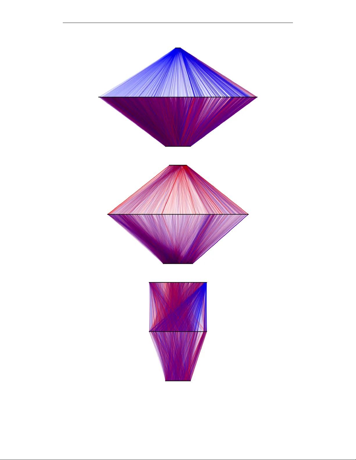
Accepted as a workshop contrib ution at ICLR 2015 D E N O I S I N G AU T O E N C O D E R W I T H M O D U L A T E D L A T E R A L C O N N E C T I O N S L E A R N S I N V A R I A N T R E P R E S E N T A T I O N S O F N A T U R A L I M A G E S Antti Rasmus and T apani Raiko Aalto Univ ersity Finland { antti.rasmus,tapani.raiko } @aalto.fi Harri V alpola ZenRobotics Ltd. V ilhonkatu 5 A, 00100 Helsinki, Finland harri@zenrobotics.com A B S T R AC T Suitable lateral connections between encoder and decoder are sho wn to allow higher layers of a denoising autoencoder (dAE) to focus on in variant represen- tations. In regular autoencoders, detailed information needs to be carried through the highest layers but lateral connections from encoder to decoder relieve this pressure. It is shown that abstract in variant features can be translated to detailed reconstructions when in variant features are allowed to modulate the strength of the lateral connection. Three dAE structures with modulated and additive lateral connections, and without lateral connections were compared in e xperiments using real-world images. The experiments v erify that adding modulated lateral connec- tions to the model 1) improves the accurac y of the probability model for inputs, as measured by denoising performance; 2) results in representations whose degree of in variance grows faster tow ards the higher layers; and 3) supports the formation of div erse inv ariant poolings. 1 I N T R O D U C T I O N Denoising autoencoders (dAE; V incent et al., 2008) provide an easily accessible method for unsu- pervised learning of representations since training can be based on simple back-propagation and a quadratic error function. An autoencoder is built from two mappings: an encoder that maps cor - rupted input data to features, and a decoder that maps the features back to denoised data as output. Thus, in its basic form, autoencoders need to store all the details about the input in its representation. Deep learning has used unsupervised pretraining (see Bengio, 2013, for a re vie w) but recently purely supervised learning has become the dominant approach at least in cases where a large number of labeled data is av ailable (e.g., Ciresan et al., 2010; Krizhevsky et al., 2012). One difficulty with combining autoencoders with supervised learning is that autoencoders try to retain all the information whereas supervised learning typically loses some. F or instance, in clas- sification of images, spatial pooling of activ ations throws away some of the location details while retaining identity details. In that sense, the unsupervised and supervised training are pulling the model in very dif ferent directions. From a theoretical perspecti ve, it is clear that unsupervised learning must be helpful at least in a semi-supervised setting. Indeed, Kingma et al. (2014) obtained very promising results with varia- tional autoencoders. This raises hopes that the same could be achie ved with simpler dAEs. Recently , V alpola (2015) proposed a variant of the denoising autoencoder that can lose informa- tion. The no velty is in lateral connections that allow higher le vels of an autoencoder to focus on in variant abstract features and in layer -wise cost function terms that allo w the netw ork to learn deep 1 Accepted as a workshop contrib ution at ICLR 2015 f (1) g (0) g (1) f (2) h (1) ˆ h (1) h (2) ˆx ˜x (a) Basic autoencoder f (1) g (0) g (1) f (2) g (2) h (1) ˆ h (1) h (2) ˜x ˆx ˆ h (2) (b) Lateral connections ↵ =0 . 25 ↵ =4 . 0 (c) Layer size ratio Figure 1: Examples of two-hidden-layer models: (a) denoising autoencoder and (b) Ladder network with lateral connections. Illustration of ratio, α , of h (2) size to h (1) size (right) with hidden layers of sizes 2 and 8. Ratio of α = 1 . 0 corresponds to hidden layers of equal size (a and b). hierarchies ef ficiently . V alpola (2015) hypothesized that modulated lateral connections support the dev elopment of in variant features and provided initial results with artificial data to back up the idea. As seen in Figure 1, information can flow from the input to the output through alternativ e routes, and the details no longer need to be stored in the abstract representation. This is a step closer to being compatible with supervised learning which can select which types of in v ariances and abstractions are relev ant for the task at hand. In this paper, we focus on inv estigating the effects of lateral connections. W e extend earlier results with experiments using natural image data and make comparisons with regular denoising autoen- coders without lateral connections in Section 2. W e show the follo wing: • The proposed structure attains a better model of the data as measured by ability to de- noise. There are good reasons to believ e that this indicates that the network has captured a more accurate probabilistic model of the data since denoising is one way of representing distributions (Bengio et al., 2013). • Including the modulated lateral connections changes the optimal balance between the sizes of layers from balanced to bottom heavy . • The degree of in variance of the representations gro ws to wards the higher lev els in all tested models but much faster with modulated lateral connections. In particular , the higher levels of the model seem to focus entirely on in variant representations whereas the higher lev els of the regular autoencoder hav e a few in variant features mixed with a large number of details. • Modulated lateral connections guide the layer above them to learn various types of pool- ings. The pooled neurons participate in se veral qualitativ ely dif ferent poolings that are each selectiv e and inv ariant to different aspects of the input. 1 . 1 I N V A R I A N T F E A T U R E S T H R O U G H P O O L I N G There are typically many sources of variation which are irrelev ant for classification. For example, in object recognition from images, these sources could include position, orientation and scale of the recognized object and illumination conditions. In order to correctly classify new samples, these sources of v ariation are disregarded while retaining information needed for discriminating between different classes. In other words, classification needs to be in v ariant to the irrelev ant transformations. A simple but naive way to achiev e such inv ariance would be to list all the possible realizations of objects under v arious transformations, but this is not usually practical due to the vast amounts of possible realizations. Also, this does not of fer any generalization to ne w objects. A useful solution is to split the generation of in variance into more manageable parts by representing the inputs in terms of features which are each in v ariant to some types of transformations. Since different kinds of objects can be represented by the same set of features, this approach makes it possible to generalize the in variances to ne w , unseen objects. So rather than listing all the possible realizations of indi vidual objects, we can list possible realiza- tions of their constituent features. Inv ariance is achiev ed by retaining only the information about 2 Accepted as a workshop contrib ution at ICLR 2015 whether any of the possible realizations is present and discarding information about which one ex- actly . Such an operation is known as pooling and there are various ways of implementing it. In the case of binary inputs, OR operation is a natural choice. There are many ways to generalize this to continuous v ariables, including maximum operation (Riesenhuber & Poggio, 1999) or summation followed by a conca ve function (Fukushima, 1979). While pooling achiev es in variance to irrelev ant transformations, the features also need to be discrim- inativ e along relev ant dimensions. This selecti vity is often achiev ed by coincidence detection, i.e. by detecting the simultaneous presence of multiple input features. In the binary case, it can be imple- mented by an AND operation. In the continuous case, possibilities include extensions of the AND operation, such as product or summation follo wed by a conv ex function, but also lateral inhibition (i.e., competition) among a set of feature detectors. All of these operations typically produce sparse coding where the output features are sensitiv e to specific combinations of input features. Since this type of coding tends to increase the number of features, it is also known as feature e xpansion. The idea of alternating pooling and feature expansion dates at least back to Hubel & W iesel (1962) who found that the early stages of visual processing in the cat cerebral cortex hav e alternating steps of feature expansion, implemented by lateral competition among so called simple cells, and in variance-generating poolings by so called complex cells. In such hierarchies of alternating steps, the degree of in variance grows towards the higher lev els. Cortical processing also includes various normalizations, a feature which has also been included in some models (e.g., Fukushima, 1979). There are various w ays of finding poolings that generate inv ariances (from specialized to general): 1. In variance by design. For instance, inv ariance to translation and small deformations is achiev ed by pooling shifted versions of a feature (Fukushima, 1979). Similar pooling op- erations are now popular in con volutional neural networks (see, e.g., Schmidhuber, 2015). 2. In variance to hand-crafted transformations. The transformations are applied to input sam- ples (e.g., image patches can be shifted, rotated, scaled or ske wed, and colors or contrast can be modified) and pooling is then learned by requiring the output to stay constant ov er the transformation. This category includes supervised learning from inputs deformed by various transformations. 3. In variance to transformations ov er time. Relies on nature to provide transformations as sequences during which the underlying feature (e.g., identity of object) changes slower than the transformation (e.g., F ¨ oldi ´ ak, 1991). 4. In variance by exploiting higher-order correlations within individual samples. This is ho w supervised learning can find poolings: target labels correlate nonlinearly with inputs. There are also unsupervised methods that can do the same. For example, subspace ICA can find complex-cell like poolings for natural images (Hyv ¨ arinen & Hoyer, 2000). W e focus on the last type: exploiting higher-order correlations. V ery few assumptions are made so the method is very general but it is also possible to combine this approach with supervised learning or any of the more specialized ways of generating in variances. 1 . 2 D E N O I S I N G AU T O E N C O D E R S Autoencoder networks have a natural propensity to conserve information and are therefore well suited for feature expansion. Autoencoder networks consist of two parameterized functions, encod- ing f and decoding g . Function f maps from input space x to feature space h , and g in turn maps back to input space producing a reconstruction, ˆ x , of the original input, when the training criterion is to minimize the reconstruction error . This enables learning of features in an unsupervised manner . Denoising autoencoder (V incent et al., 2008) is a variant of the traditional autoencoder, where the input x is corrupted with noise and the objective of the network is to reconstruct the original un- corrupted input x from the corrupted ˜ x . Bengio et al. (2013) show that denoising autoencoders implicitly estimate the data distribution as the asymptotic distribution of the Markov chain that alternates between corruption and denoising. This interpretation provides a solid probabilistic foun- dation for them. Consequently , the denoising teaching criterion enables learning of ov er-complete representations, a property which is crucial for adding lateral connections to an autoencoder . 3 Accepted as a workshop contrib ution at ICLR 2015 As with normal feedforward networks, there are various options for choosing the cost function but, in the case of continuous input variables, a simple choice is C = k ˆ x − x k 2 = k g ( f ( ˜ x )) − x k 2 . (1) Denoising autoencoders can be used to build deep architectures either by stacking sev eral on top of each other and training them in a greedy layer-wise manner (e.g., Bengio et al., 2007) or by chaining sev eral encoding and decoding functions and training all layers simultaneously . F or L layers and encoding functions f ( l ) , the encoding path would compose as f = f ( L ) ◦ f ( L − 1) ◦ . . . f (1) . W e denote the intermediate feature v ectors by h ( l ) and corresponding decoded, denoised, v ectors by ˆ h ( l ) . Figure 1a depicts such a structure for L = 2 . Encoding functions are of the form h ( l ) = f ( l ) ( h ( l − 1) ) = φ  W ( l ) f h ( l − 1) + b ( l ) f  , 1 ≤ l ≤ L, (2) starting from h (0) = ˜ x . The corresponding decoding functions are ˆ h ( L ) = h ( L ) (3) ˆ h ( l ) = g ( l ) ( ˆ h ( l +1) ) = φ  W ( l ) g ˆ h ( l +1) + b ( l ) g  , 1 ≤ l ≤ L − 1 , (4) ˆ x = g (0) ( ˆ h (1) ) = W (0) g ˆ h (1) + b (0) g . (5) Function φ is the activ ation function and typically left out from the lowest layer . 2 E X P E R I M E N T S The tendency of regular autoencoders to preserve information seems to be at odds with the de- velopment of in variant features which relies on poolings that selectively discard some types of information. Our goal here is to in vestigate the hypothesis that suitable lateral connections allow autoencoders to discard details from higher layers and only retain abstract in variant features because the decoding functions g ( l ) can recov er the discarded details from the encoder . W e compare three different denoising autoencoder structures: basic denoising autoencoder and two variants with lateral connections. W e experimented with various model definitions prior to deciding the ones defined in Section 2.1 because there are multiple ways to mer ge lateral connections. 2 . 1 M O D E L S W I T H L A T E R A L C O N N E C T I O N S W e add lateral connections from h ( l ) to ˆ h ( l ) as seen in Figure 1b. Autoencoders trained without noise would short-circuit the input and output with an identity mapping. No w that input contains noise, there is pressure to find meaningful higher-le vel representations that capture regularities and allow for denoising. Note that the encoding function f has the same form as before in Eq. (2). 2 . 1 . 1 A D D I T I V E L A T E R A L C O N N E C T I O N S As the first version, we replace the decoding functions in Eq. (3 – 4) with ˆ h ( L ) = g ( L ) ( h ( L ) ) = ( h ( L ) + b ( L ) a )  σ  a ( L )  h ( L ) + b ( L ) b  , (6) ˆ h ( l ) = g ( l ) ( h ( l ) , ˆ h ( l +1) ) = ( h ( l ) + b ( l ) a )  σ  a ( l )  h ( l ) + b ( l ) b  + φ  W ( l ) g ˆ h ( l +1) + b ( l ) g  , (7) where  is the element-wise (i.e., Hadamard) product, a ( l ) , b ( l ) a , and b ( l ) b are learnable parameter vectors along with weights and biases, and σ is a sigmoid function to ensure that the modulation stays within reasonable bounds. Function g (0) stays af fine as in Eq. (5). The functional form of Eq. (6), with element-wise decoding, is motiv ated by element-wise denoising functions that are used in denoising source separation (S ¨ arel ¨ a & V alpola, 2005) and corresponds to assuming the elements of h independent a priori. 4 Accepted as a workshop contrib ution at ICLR 2015 2 . 1 . 2 M O D U L A T E D L AT E R A L C O N N E C T I O N S Our hypothesis is that an autoencoder can learn inv ariances efficiently only if its decoder can make good use of them. V alpola (2015) proposed connecting the top-down mapping inside the sigmoid term of Eq. (7), a choice motiv ated by optimal denoising in hierarchical variance models. Our final proposed model includes the encoding functions in Eq. (2), the top connection g ( L ) in Eq. (6), bottom decoding function g (0) as in Eq. (5), but the middle decoding functions are defined as g ( l ) ( h ( l ) , ˆ h ( l +1) ) = ( h ( l ) + b ( l ) a )  σ  a ( l )  h ( l ) + W ( l ) g ˆ h ( l +1) + b ( l ) b  , 1 ≤ l ≤ L − 1 . (8) In contrast to additive lateral connection in Eq. (7), the signal from the abstract layer ˆ h ( l +1) is used to modulate the lateral connection so that the top-do wn connection has mo ved from φ ( · ) to σ ( · ) , and the bias b ( l ) g has dropped because it is redundant with the bias term b ( l ) b in σ ( · ) . Modulated (also kno wn as gated or three-way) connections have been used in autoencoders before but in a rather different context. Memisevic (2011) uses a weight tensor to connect two inputs to a feature. W e connect the i th component of h ( l ) only to the i th component of ˆ h ( l ) , keeping the number of additional parameters small. 2 . 2 T R A I N I N G P RO C E D U R E In order to compare the models, we optimized each model structure constraining to 1 million pa- rameters and 1 million mini-batch updates to find the best denoising performance, that is, the lowest reconstruction cost C in Eq. (1). The better the denoising performs the better the implicit probabilis- tic model is. The tasks is the same for all models, so the comparison is fair . W ith two-layer models ( L = 2 ) the focus w as to find the optimal size for layers, especially the ratio of h (2) size to h (1) size (see Fig. 1c for the definition of the ratio α ). All the models use rectified linear unit as the acti vation function φ ( · ) and the noise was Gaussian with zero mean and standard deviation scaled to be 50% of that of the data. In order to find the best possible baseline for comparison, we e valuated weight tying for autoencoder without lateral connections , that is, W ( l ) g = W ( l +1) f T , and noticed that tying weights resulted in faster con ver gence and thus better denoising performance than without weight tying. Howe ver , when combining both so that weights are tied in the be ginning and untied for the latter half of the training, denoising performance improv ed slightly (by 1% ), b ut did not affect the relativ e difference of v arious models. Since weight tying had only negligible impact on the results, but it complicates training and reproducibility , we designed the experiments so that all models use tied weights counting tied weights as separate parameters. Results of the denoising performance are described in Section 2.3. W e performed the analysis on natural images because the in variances and learned features are easy to visualize, we kno w beforehand that such in variances do exist, and because computer vision is an important application field in its own right. W e used 16 × 16 patches from two image datasets: CIF AR-10 (Krizhe vsky & Hinton, 2009) and natural images used by Olshausen & Field (1996) 1 . W e refer to this dataset as O&F . The training length was limited to 1 million mini-batch updates with mini-batch of size 50 and learn- ing rate was adapted with AD ADEL T A (Zeiler, 2012). The best v ariants of each model were then trained longer , for 4 million updates, and further analyzed to determine in v ariance of the learned rep- resentations. This is described and reported in Section 2.4. Supplementary material provides more details about data preprocessing, division between training and validation sets, training procedure, hyperparameters used with AD ADEL T A, and how weights were initialized. W e also tried stacked layer-wise training by training each layer for 500,000 updates followed by fine- tuning phase of another 500,000 updates such that the total number of updates for each parameter equals to 1 million. W e also tried a local cost function and noise source on each layer or using the global cost, but we did not find any such stacked training beneficial compared to the direct simultaneous training of all layers, which is what we report in this paper . 1 A vailable at https://redwood.berkeley.edu/bruno/sparsenet/ 5 Accepted as a workshop contrib ution at ICLR 2015 0 . 0 0 . 1 0 . 2 0 . 3 0 . 4 0 . 5 1 . 0 2 . 0 3 . 0 α 0 . 16 0 . 18 0 . 20 Cost Mo d No-lat Add 0 . 0 0 . 1 0 . 2 0 . 3 0 . 4 0 . 5 1 . 0 2 . 0 3 . 0 α 0 . 115 0 . 120 0 . 125 Cost Mo d No-lat Add Figure 2: The best validation cost per element as a function of α , the ratio of h (2) size to h (1) size, for CIF AR-10 (left) and O&F (right) datasets. Dotted line is the result of linear denoising (model Linear in T able 1), two dashed lines represent the denoising performance of one-layer models ( L = 1) with and without lateral connections according to their colors. Note that Add and Mod models are identical when L = 1 . The scale of the horizontal axis is linear until 0.5 and logarithmic after that. 10 − 2 10 − 1 10 0 0 . 0 0 . 2 0 . 4 0 . 6 0 . 8 1 . 0 γ (2) i Mod 256-1622-50 10 − 2 10 − 1 10 0 Add 25 6 -839 -336 10 − 2 10 − 1 10 0 No-lat 256-590-589 Figure 3: Translation in v ariance measure of neurons on h (2) as a function of significance. Color indicates the av erage sign of the connected weights from negati ve (blue) to positive (red). Best viewed in color . See Section 2.4 for more details. 2 . 3 D E N O I S I N G P E R F O R M A N C E The results of denoising performance for models with one and tw o layers is presented in the Figure 2 which shows the lowest reconstruction cost on a validation dataset for both datasets. Each configu- ration was trained 5 times with different random initialization for confidence bounds calculated as corrected sample standard deviation of the lo west reconstruction cost. The best performing No-lat model (autoencoder without lateral connections) is a one-layer model and is shown in dashed line. The best two-layer No-lat models in CIF AR-10 and O&F have ratios of α min = 1 . 0 and α min = 1 . 4 , respectiv ely . Since No-lat autoencoders need to push all the information through each layer , it is intuitiv e that very narrow bottlenecks are bad for the model, that is, large and small ratios perform poorly . A further study of why the optimal ratio is larger for O&F revealed that the lo wer layer can be smaller because the effecti ve dimensionality in terms of principal components is lo wer for O&F compared to CIF AR-10. Second layer is not beneficial with No-lat model giv en the parameter number constraint. Mod (modulated lateral connections) model benefits from the second layer and works best when the ratio is small, namely α min = 0 . 03 and α min = 0 . 12 for CIF AR-10 and O&F , respecti vely . The second layer does not hurt or benefit Add (additive lateral connection) model significantly and its performance is between No-lat and Mod models. The results are also presented as numbers in T able 1 in supplementary material. 6 Accepted as a workshop contrib ution at ICLR 2015 2 . 4 R E S U L T I N G I N V A R I A N T F E A T U R E S Practically no prior information about poolings was incorporated in either the model structure or treatment of training data. This means that any in variances learned by the model must hav e been present in the higher-order correlations of the inputs, as explained in Section 1.1. It is well known that such inv ariances can be de veloped from natural images (e.g., Hyv ¨ arinen & Hoyer, 2000) but the question is, how well are the dif ferent model structures able to represent and learn these features. T o test this, we generated sets of rotated, scaled and translated images and measured ho w inv ariant the activ ations h ( l ) are for each type of transformation separately . As an example for translation, each set contained 16 translated images (from a 4 × 4 grid). For each set s in a gi ven transformation type, we calculated the mean activ ation h h ( l ) i s and compared their variances with the v ariance v ar { h ( l ) } ov er all samples: γ ( l ) i = v ar {h h ( l ) i i s } / v ar { h ( l ) i } . (9) From the definition it follows that 0 ≤ γ ( l ) i ≤ 1 . If the feature is completely in variant with respect to the transformation, γ ( l ) i equals one 2 . As the overall conclusions are similar to all tested transfor- mations, the main text concentrates on the translation in variance. Results for other in variances are reported in supplementary material, Section 4.4. The average layer-wise in v ariance, γ ( l ) = h γ ( l ) i i i , grows tow ards the higher layers in all models but much faster in the best Mod models than in others 3 , i.e. for CIF AR-10 the best Mod model has γ (0) ... (2) = (0 . 20 , 0 . 31 , 0 . 84) , whereas for the best No-lat γ (0) ... (2) = (0 . 20 , 0 . 23 , 0 . 30) . All γ ( l ) values are reported in T able 1 in supplementary material. T o further illustrate this, we plotted in Figure 3 the in v ariance measures γ (2) i for the best variant of each model. In each plot, dots correspond to hidden neurons h (2) i and the color reflects the average sign of the encoder connection to that neuron (blue for negati ve, red for positive). The horizontal axis is the significance of a neuron, a measure of how much the model uses that hidden neuron, which is defined and analyzed in supplementary material, Section 4.3. There are two notable observ ations. First, all h (2) i neurons of Mod model are highly in variant, whereas the other models have only fe w in variant neurons and the vast majority of neurons hav e very low in variance. For No-lat model, in variance seems to be even smaller for those neurons that the model uses more. Moreover , we tested that the second layer of Mod model stays highly in variant ev en if the layer size is increased (shown in Figure 7c in supplementary material). Second, in variant neurons tend to hav e far more and stronger negativ e than positive weights, especially so with Mod and No-lat models. Since the nonlinearity φ ( x ) on each layer was the rectified linear unit, a conv ex function which saturates on the negati ve side, negati ve tied weights mean that the network flipped these functions into − φ ( − x ) , that is, conca ve functions that saturate on the positiv e side resembling OR operation. This interpretation is further discussed in supplementary material, Section 4.3.2. 2 . 5 L E A R N E D P O O L I N G S The modulated Mod model used practically all of the second layer neurons for pooling. When study- ing the poolings, we found that typically e very Layer 1 neuron participates in several qualitati vely different poolings. As can be seen from the Figure 4, each Layer 1 neuron (sho wn on the left-most column) participates in different kinds of poolings each of which is sensitiv e to a particular set of features and in variant to other types. F or example, Layer 1 neuron (c) is selecti ve to orientation, frequency and color but it participates in three different Layer 2 poolings . The first one is selecti ve to color b ut in variant to orientation. The second one is selectiv e to orientation b ut in variant to color . The third one only responds to high frequency and orientation. More details of the analysis are av ailable in supplementary material. 2 V arious measures of inv ariance ha ve been proposed (e.g., Goodfellow et al., 2009). Our in v ariance measure γ is closely related to autocorrelation which has been used to measure in variance, e.g., by Dosovitskiy et al. (2014). The set of translated patches includes pairs with various translations and therefore our measure is a weighted av erage of the autocorrelation function. The wider the autocorrelation, the larger the measure γ . 3 Our measure γ can be fooled by copying the same in variant feature to man y hidden neurons but we verified that this is not happening here: slow feature analysis is robust against such redundancy but yields qualitativ ely the same results for the tested networks. 7 Accepted as a workshop contrib ution at ICLR 2015 (a) (b) (c) (d) Figure 4: V arious pooling groups a neuron. Each set (a)-(d) represents three rele vant pooling groups the selected neuron h (1) a . . . h (1) d , depicted in the first column, belongs to. Each row represents an h (2) pooling neuron by showing the 20 most relev ant h (1) neurons associated with it. Poolings were found by selecting a few Layer 1 neurons and follo wing their strongest links to Layer 2 to identify the poolings in which they participate. Consecutiv ely , the Layer 1 neurons corresponding to each pooling group were identified by walking back the strongest links from each Layer 2 neuron. Best viewed in color . The procedure of choosing features in the plot is also depicted in Figure 8 in supplementary material. 3 D I S C U S S I O N The experiments showed that in variance in denoising autoencoders increased towards the higher lay- ers but significantly so only if the decoder had a suitable structure where details could be combined with inv ariant features via multiplicative interactions. Lateral connections from encoder to decoder allowed the models to discard details from the higher lev els but only if the details and in v ariant features were combined suitably . The best models with modulated lateral connections were able to learn a lar ge number of poolings in an unsupervised manner . W e tested their inv ariance but nothing in the model biased learning in that direction and we observed in variance and selecti ve discrimination of sev eral different dimensions such as color , orientation and frequency . In summary , these findings are fully in line with the earlier proposition that the unsupervised denois- ing autoencoder with modulated lateral connections can work in tandem with supervised learning because, as we hav e shown here for the first time, the higher layers of the model hav e the ability to focus on abstract representations and, unlike re gular autoencoders, should therefore be able to discard details if supervised learning deems them irrelev ant. It now becomes possible to combine autoencoders with the popular supervised learning pipelines which include in-built pooling opera- tions (see, e.g., Schmidhuber, 2015). There are multiple w ays to extend the w ork, including 1) e xplicit bias to wards in variances; 2) sparse structure such as con volutional networks, making much larger scale models and deeper hierarchies feasible; 3) dynamic models; and 4) semi-supervised learning. R E F E R E N C E S Bengio, Y , Lamblin, P , Popovici, D, and Larochelle, H. Greedy layer-wise training of deep networks. In Advances in Neural Information Pr ocessing Systems (NIPS 2006) , 2007. 8 Accepted as a workshop contrib ution at ICLR 2015 Bengio, Y . Deep learning of representations: Looking forward. In Statistical Language and Speech Pr ocessing , pp. 1–37. Springer, 2013. Bengio, Y , Y ao, L, Alain, G, and V incent, P . Generalized denoising auto-encoders as generati ve models. In Advances in Neural Information Pr ocessing Systems , pp. 899–907, 2013. Ciresan, D. C, Meier, U, Gambardella, L. M, and Schmidhuber, J. Deep big simple neural nets for handwritten digit recogntion. Neural Computation , 22(12):3207–3220, 2010. Dosovitskiy , A, Springenberg, J. T , Riedmiller , M, and Brox, T . Discriminative unsupervised feature learning with con volutional neural networks. In Ghahramani, Z, W elling, M, Cortes, C, Lawrence, N, and W einberger , K (eds.), Advances in Neural Information Pr ocessing Systems (NIPS 2014) , pp. 766–774. 2014. F ¨ oldi ´ ak, P . Learning inv ariance from transformation sequences. Neural Computation , 3:194–200, 1991. Fukushima, K. Neural netw ork model for a mechanism of pattern recognition unaf fected by shift in position - Neocognitron. T rans. IECE , J62-A(10):658–665, 1979. Goodfellow , I, Lee, H, Le, Q. V , Saxe, A, and Ng, A. Y . Measuring in variances in deep networks. In Advances in Neural Information Pr ocessing Systems (NIPS) , pp. 646–654, 2009. Hubel, D. H and W iesel, T . N. Receptive fields, binocular interaction and functional architecture in the cat’ s visual cortex. The J ournal of physiology , 160(1):106, 1962. Hyv ¨ arinen, A and Hoyer , P . Emergence of phase-and shift-in variant features by decomposition of natural images into independent feature subspaces. Neural computation , 12(7):1705–1720, 2000. Kingma, D. P , Mohamed, S, Rezende, D. J, and W elling, M. Semi-supervised learning with deep generativ e models. In Ghahramani, Z, W elling, M, Cortes, C, Lawrence, N, and W einberger , K (eds.), Advances in Neural Information Pr ocessing Systems (NIPS 2014) , pp. 3581–3589. Curran Associates, Inc., 2014. Krizhevsk y , A and Hinton, G. Learning multiple layers of features from tiny images. T echnical report, Univ ersity of T oronto, 2009. Krizhevsk y , A, Sutske ver , I, and Hinton, G. E. ImageNet classification with deep con volutional neural networks. In Advances in Neural Information Pr ocessing Systems (NIPS 2012) , pp. 1106– 1114, 2012. Memisevic, R. Gradient-based learning of higher-order image features. In 2011 IEEE International Confer ence on Computer V ision (ICCV) , pp. 1591–1598, November 2011. Olshausen, B. A and Field, D. J. Emergence of simple-cell receptiv e field properties by learning a sparse code for natural images. Natur e , 381:607–609, 1996. Raiko, T , V alpola, H, and LeCun, Y . Deep learning made easier by linear transformations in percep- trons. In La wrence, N. D and Girolami, M (eds.), AIST ATS , volume 22 of JMLR Pr oceedings , pp. 924–932. JMLR.org, 2012. Riesenhuber , M and Poggio, T . Hierarchical models of object recognition in cortex. Nature Neur o- science , 2(11):1019–1025, 1999. S ¨ arel ¨ a, J and V alpola, H. Denoising source separation. Journal of Machine Learning Resear ch , 6: 233–272, 2005. Schmidhuber , J. Deep learning in neural networks: an ov erview . Neural Networks , 61:85–117, 2015. V alpola, H. From neural PCA to deep unsupervised learning. In Advances in Independent Compo- nent Analysis and Learning Machines . Else vier, 2015. Preprint a v ailable as V incent, P , Larochelle, H, Bengio, Y , and Manzagol, P .-A. Extracting and composing rob ust features with denoising autoencoders. T echnical Report 1316, Universit ´ e de Montr ´ eal, dept. IR O, 2008. Zeiler , M. D. Adadelta: An adapti ve learning rate method. arXiv pr eprint arXiv:1212.5701 , 2012. 9 Accepted as a workshop contrib ution at ICLR 2015 T able 1: Denoising performance and translation inv ariance measure of selected models. All models hav e exactly the same input layer and data so the av erage in variance is the same for all models, e.g. for CIF AR-10, γ (0) = 0 . 20 . Dataset Model Layer sizes Ratio α Min cost ± std In variance, γ ( l ) CIF AR-10 Linear 256 0.20316 ± 0.00011 N A CIF AR-10 No-lat 256-1948 0.00 0.16144 ± 0.00007 0.20, 0.29 CIF AR-10 Add/Mod 256-1937 0.00 0.15793 ± 0.00007 0.20, 0.29 CIF AR-10 No-lat 256-590-589 1.00 0.17595 ± 0.00034 0.20, 0.23, 0.30 CIF AR-10 Add 256-839-336 0.40 0.15734 ± 0.00015 0.20, 0.27, 0.33 CIF AR-10 Mod 256-1622-50 0.03 0.15086 ± 0.00022 0.20, 0.31, 0.84 O&F Linear 256 0.14686 ± 0.00010 N A O&F No-lat 256-1948 0.00 0.12290 ± 0.00008 0.16, 0.24 O&F Add/Mod 256-1937 0.00 0.11891 ± 0.00006 0.16, 0.25 O&F No-lat 256-512-718 1.40 0.12446 ± 0.00015 0.16, 0.19, 0.27 O&F Add 256-1061-212 0.20 0.11723 ± 0.00009 0.16, 0.25, 0.41 O&F Mod 256-1395-100 0.07 0.11234 ± 0.00005 0.16, 0.24, 0.95 4 S U P P L E M E N TA RY M AT E R I A L 4 . 1 P R E P RO C E S S I N G O F DAT A Patches of size 16 × 16 were sampled randomly and continuously during training. Separate test images were put aside for testing generalization performance: the last 10,000 samples for CIF AR- 10 and the sixth image of O&F dataset. Continuous sampling allows generation of millions of data samples alleviating overfitting problems. O&F dataset was already (partially) whitened so no further preprocessing was applied to it. RGB color patches of CIF AR-10 were whitened and dimensionality was reduced to 256 with PCA to match the dimensionality of grayscale images of O&F . Despite dimensionality reduction, 99% of the variance w as retained. 4 . 2 D E TA I L S O F T H E T R A I N I N G P RO C E D U R E White additiv e Gaussian noise of σ N = 0 . 5 was used for corrupting the inputs which were scaled to hav e standard deviation of σ = 1 . 0 . During training, AD ADEL T A was used to adapt the learning rate with its momentum set to 0 . 99 , and  = 10 − 8 . All weight vectors were initialized from normal distribution to have a norm of 1 . 0 , and orthogonalized. In order to improve the conv ergence speed of all models, we centered the hidden unit activ ations following Raiko et al. (2012): there is an auxiliary bias term β (Raiko et al., 2012, Eq. (2)), applied immediately after the nonlinearity , that centers the output to zero mean. 4 4 . 3 A N A L Y S I S O F M A P P I N G S W e analyzed the mappings learned by different types of models in several ways and present here some of the most interesting findings. First, it turned out that dif ferent models had very dif ferent proportions of inv ariant neurons on h (2) (in variance measure γ is defined in Eq. (9)) and we wanted to understand better what w as going on. Some key questions were ho w important roles different types of features had and how the in v ariances were formed. Second level in variances could be low-frequenc y features which are in variant already on the first layer (and thus not particularly interesting) or formed through pooling Layer 1 neurons. The first question can be answered by looking at where the connections are coming from. The connections W ( l ) g are visualized in Figures 5a – 5c. The neurons on each layer hav e been ordered with respect to inv ariance which increases from left to right. The connecting edges have been colored according to the sign of the connecting weight and the strength of each edge reflects the significance of the connection. Significance is defined as the proportion of variance that the higher-le vel neuron 4 W e did not use the other transformation α since it would ha ve required shortcut connections. 10 Accepted as a workshop contrib ution at ICLR 2015 generates on the lo wer-lev el neurons. W e initially tried visualizing simply the magnitudes of the weights but the problem is that when an input neuron has a low variance or the output neuron is saturated, a large weight magnitude does not indicate that the connection is important; it would not make much dif ference if such a connection were removed. 4 . 3 . 1 S I G N I FI C A N C E M E A S U R E When visualizing W ( l ) g , we first took the squares and scaled them by the input neuron’ s variance v ar { h ( l +1) i } . Assuming input neurons are independent, this quantity reflects the input variance each neuron h ( l ) j receiv es. Depending on the saturation of the neuron, a smaller or greater proportion of this v ariance is transmitted to the actual output variance v ar { h ( l ) j } . W e therefore scaled all the incoming v ariances for each h ( l ) j such that their sum matches the output v ariance v ar { h ( l ) j } . W e named this quantity the significance of the connection and it approximately measures where the output variance of each layer originates from. This significance is also depicted in Figure 3 where the x coordinate is the sum of output significances for each h (2) i . 4 . 3 . 2 R O L E O F N E G A T I V E W E I G H T S It turned out that the in variant neurons tend to hav e far more and stronger negati ve than positi ve weights. W e visualized this with color in Figure 5: blue signifies negativ e and red positiv e weights. In the images, the connections are translucent which means that equal number (and significance) of positiv e and negativ e weights results in purple color . A striking feature of these plots is that the most in variant features tend to hav e all negati ve weights. Since the nonlinearity φ ( x ) on each layer was the rectified linear unit, a conv ex function which saturates on the negati ve side, negati ve tied weights mean that the network flipped these functions into − φ ( − x ) , that is, concave functions that saturate on the positiv e side. It therefore looks like the network learned to add a layer of concave OR-like in variance-generating poolings on top of con vex AND-like coincidence detectors. Forming con vex AND using positiv e weights and concave OR using negati ve weights is demonstrated respecti vely as truth tables in T able 2 and T able 3, and the geometric form is illustrated in Figure 6a and Figure 6b. 4 . 4 I N V A R I A N C E W e also studied inv ariance of the second layer neurons for scaling and rotation transformations using the same in variance measure as defined in Section 2.4 for translation. W e formed sets of 16 samples by scaling CIF AR-10 images with a zoom factors 0 . 6 , 0 . 65 , . . . , 1 . 35 and rotating images − 32 ◦ , − 28 ◦ , . . . , 28 ◦ for scaling and rotation in variance experiments, respectiv ely . The results are shown in Figure 7a and Figure 7b and are similar to the translation in variance in Figure 3. Figure 7c illustrates the impact of increasing α , i.e. increasing the size of the second layer . Notably all second layer neurons stay highly in variant e ven when the layer size is increased. 11 Accepted as a workshop contrib ution at ICLR 2015 (a) Connections of Mod model 256-1622-50 (b) Connections of Add model 256-839-336. (c) Connections of No-lat model 256-590-589. Figure 5: Neurons are ordered according to increasing translation in variance from left to right. Blue denotes ne gative and red positi ve weights in W ( l ) g . Strength of the connections depends on the significance of the connection (see text for details). Layer 2 neurons of this model are also visualized in Figure 3. Best vie wed in color . 12 Accepted as a workshop contrib ution at ICLR 2015 T able 2: T ruth table for logical AND operation giv en three-element binary input vector x and a single perceptron with ReLU activ ation function φ ( · ) . φ ( z ) = φ ( x T w + b ) = φ ( x 0 w 0 + x 1 w 1 + x 2 w 2 + b ) x 0 x 1 x 2 w i b z φ ( z ) AND 0 0 0 1 -2 -2 0 0 0 0 1 1 -2 -1 0 0 0 1 0 1 -2 -1 0 0 0 1 1 1 -2 0 0 0 1 0 0 1 -2 -1 0 0 1 0 1 1 -2 0 0 0 1 1 0 1 -2 0 0 0 1 1 1 1 -2 1 1 1 T able 3: Truth table for logical OR operation gi ven three-element binary input vector x and a single perceptron with ReLU activ ation function φ ( · ) . φ ( z ) = φ ( x T w + b ) = φ ( x 0 w 0 + x 1 w 1 + x 2 w 2 + b ) x 0 x 1 x 2 w i b z φ ( z ) 1 − φ ( z ) NOR OR 0 0 0 -1 1 1 1 0 1 0 0 0 1 -1 1 0 0 1 0 1 0 1 0 -1 1 0 0 1 0 1 0 1 1 -1 1 -1 0 1 0 1 1 0 0 -1 1 0 0 1 0 1 1 0 1 -1 1 -1 0 1 0 1 1 1 0 -1 1 -1 0 1 0 1 1 1 1 -1 1 -2 0 1 0 1 0 1 2 3 Number of activ e inputs 0 1 2 Conv ex AND fu nction (a) Function φ ( x T w + b ) , w i = 1 , b = − 2 0 1 2 3 Number of activ e inputs 0 1 2 Concav e OR fu nction (b) Function 1 − φ ( x T w + b ) , w i = − 1 , b = 1 Figure 6: Conceptual illustration of linear rectifier unit, φ ( · ) , performing logical AND and OR operations for three-element binary input x , x i ∈ { 0 , 1 } after the affine transform z = x T w + b = x 0 w 0 + x 1 w 1 + x 2 w 2 + b . AND operations has positive weights and con ve x form, whereas OR operation has negati ve weights and concav e functional form. 13 Accepted as a workshop contrib ution at ICLR 2015 10 − 2 10 − 1 10 0 0 . 0 0 . 2 0 . 4 0 . 6 0 . 8 1 . 0 γ (2) i Mod 256-1622-50 10 − 2 10 − 1 10 0 Add 25 6 -839 -336 10 − 2 10 − 1 10 0 No-lat 256-590-589 (a) Rotation in variance 10 − 2 10 − 1 10 0 0 . 0 0 . 2 0 . 4 0 . 6 0 . 8 1 . 0 γ (2) i Mod 256-1622-50 10 − 2 10 − 1 10 0 Add 25 6 -839 -336 10 − 2 10 − 1 10 0 No-lat 256-590-589 (b) Scaling in variance 10 − 3 10 − 2 10 − 1 10 0 0 . 0 0 . 2 0 . 4 0 . 6 0 . 8 1 . 0 γ (2) i Mod 256-1622-50 10 − 3 10 − 2 10 − 1 10 0 Mod 256-1500-75 10 − 3 10 − 2 10 − 1 10 0 Mod 256-1395-100 (c) T ranslation in variance for Mod models with larger α Figure 7: V arious in variance measures for neurons of h (2) as a function of significance for CIF AR- 10. Color indicates the av erage sign of the connected weights from negati ve (blue) to positi ve (red). Best viewed in color . See Section 2.4 for more details. 14 Accepted as a workshop contrib ution at ICLR 2015 Figure 8: Method for selecting pooling groups including a giv en h (1) neuron contains two phases. First, follo w the strongest links up to the second layer to identify 3 pooling groups the first-layer neuron belongs to (left). Second, visualize each pooling group by identifying the Layer 1 neurons that have the strongest links back from each Layer 2 neuron (right). In this e xample, the first pooling group contains neurons mark ed with green, the second pooling group with red, and the third consist of purple neurons. Colors correspond to rows in Figure 4 and both phases were performed for each set (a)-(d). 15