The No-U-Turn Sampler: Adaptively Setting Path Lengths in Hamiltonian Monte Carlo

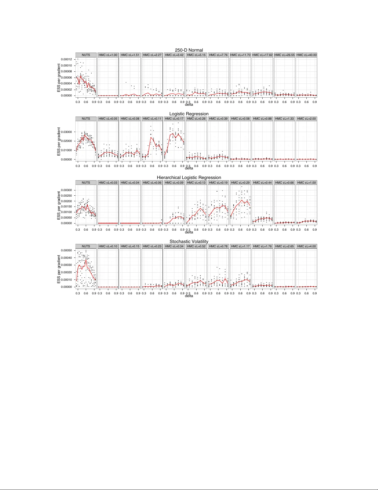
The No-U-Turn Sampler The No-U-T urn Sampler: Adaptiv ely Setting P ath Lengths in Hamiltonian Mon te Carlo Matthew D. Hoﬀman mdhoffma@cs.princeton.edu Dep artment of Statistics Columbia University New Y ork, NY 10027, USA Andrew Gelman gelman@st a t.columbia.edu Dep artments of Statistics and Politic al Scienc e Columbia University New Y ork, NY 10027, USA Abstract Hamiltonian Monte Carlo (HMC) is a Mark ov c hain Mon te Carlo (MCMC) algorithm that a voids the random w alk b eha vior and sensitivit y to correlated parameters that plague many MCMC metho ds by taking a series of steps informed by ﬁrst-order gradient information. These features allo w it to conv erge to high-dimensional target distributions muc h more quic kly than simpler methods such as random w alk Metrop olis or Gibbs sampling. Ho wev er, HMC’s p erformance is highly sensitiv e to tw o user-sp eciﬁed parameters: a step size  and a desired n umber of steps L . In particular, if L is to o small then the algorithm exhibits undesirable random w alk b eha vior, while if L is too large the algorithm wastes computation. W e introduce the No-U-T urn Sampler (NUTS), an extension to HMC that eliminates the need to set a n umber of steps L . NUTS uses a recursive algorithm to build a set of likely candidate p oints that spans a wide swath of the target distribution, stopping automatically when it starts to double bac k and retrace its steps. Empirically , NUTS p erform at least as eﬃcien tly as and sometimes more eﬃcien tly than a well tuned standard HMC metho d, without requiring user in terven tion or costly tuning runs. W e also derive a metho d for adapting the step size parameter  on the ﬂy based on primal-dual av eraging. NUTS can thus b e used with no hand-tuning at all. NUTS is also suitable for applications suc h as BUGS-style automatic inference engines that require eﬃcient “turnkey” sampling algorithms. Keyw ords: Mark ov chain Monte Carlo, Hamiltonian Monte Carlo, Ba yesian inference, adaptiv e Mon te Carlo, dual a veraging. 1. In tro duction Hierarc hical Bay esian mo dels are a mainstay of the machine learning and statistics com- m unities. Exact p osterior inference in such models is rarely tractable, how ev er, and so researc hers and practitioners must usually resort to appro ximate statistical inference meth- o ds. Deterministic appro ximate inference algorithms (for example, those review ed b y W ain- wrigh t and Jordan (2008)) can b e eﬃcient, but introduce bias and can b e diﬃcult to apply to some models. Rather than computing a deterministic approximation to a target p oste- rior (or other) distribution, Marko v chain Mon te Carlo (MCMC) metho ds oﬀer schemes for dra wing a series of correlated samples that will conv erge in distribution to the target distri- 1 Hoffman and Gelman bution (Neal, 1993). MCMC metho ds are sometimes less eﬃcien t than their deterministic coun terparts, but are more generally applicable and are asymptotically un biased. Not all MCMC algorithms are created equal. F or complicated mo dels with man y param- eters, simple metho ds such as random-walk Metrop olis (Metrop olis et al., 1953) and Gibbs sampling (Geman and Geman, 1984) ma y require an unacceptably long time to conv erge to the target distribution. This is in large part due to the tendency of these metho ds to explore parameter space via ineﬃcien t random w alks (Neal, 1993). When mo del parameters are con tinuous rather than discrete, Hamiltonian Mon te Carlo (HMC), also kno wn as hybrid Mon te Carlo, is able to suppress suc h random walk b eha vior by means of a clever auxiliary v ariable scheme that transforms the problem of sampling from a target distribution in to the problem of simulating Hamiltonian dynamics (Neal, 2011). The cost of HMC p er indep en- den t sample from a target distribution of dimension D is roughly O ( D 5 / 4 ), which stands in sharp contrast with the O ( D 2 ) cost of random-walk Metrop olis (Creutz, 1988). HMC’s increased eﬃciency comes at a price. First, HMC requires the gradient of the log-p osterior. Computing the gradien t for a complex mo del is at b est tedious and at worst imp ossible, but this requiremen t can b e made less onerous b y using automatic diﬀeren tiation (Griew ank and W alther, 2008). Second, HMC requires that the user sp ecify at least t wo parameters: a step size  and a num b er of steps L for whic h to run a simulated Hamiltonian system. A p o or choice of either of these parameters will result in a dramatic drop in HMC’s eﬃciency . Methods from the adaptiv e MCMC literature (see Andrieu and Thoms (2008) for a review) can be used to tune  on the ﬂy , but setting L typically requires one or more costly tuning runs, as w ell as the exp ertise to in terpret the results of those tuning runs. This h urdle limits the more widespread use of HMC, and mak es it challenging to incorp orate HMC into a general-purp ose inference engine such as BUGS (Gilks and Spiegelhalter, 1992), JA GS (h ttp://mcmc-jags.sourceforge.net), Infer.NET (Mink a et al.), HBC (Daume I I I, 2007), or PyMC (Patil et al., 2010). The main con tribution of this paper is the No-U-T urn Sampler (NUTS), an MCMC algorithm that closely resembles HMC, but eliminates the need to c ho ose the problematic n umber-of-steps parameter L . W e also provide a new dual av eraging (Nesterov, 2009) sc heme for automatically tuning the step size parameter  in b oth HMC and NUTS, making it p ossible to run NUTS with no hand-tuning at all. W e will sho w that the tuning-free v ersion of NUTS samples as eﬃciently as (and sometimes more eﬃciently than) HMC, even ignoring the cost of ﬁnding optimal tuning parameters for HMC. Th us, NUTS brings the eﬃciency of HMC to users (and generic inference systems) that are unable or disinclined to sp end time tw eaking an MCMC algorithm. 2. Hamiltonian Mon te Carlo In Hamiltonian Mon te Carlo (HMC) (Neal, 2011, 1993; Duane et al., 1987), w e in tro duce an auxiliary momentum v ariable r d for each mo del v ariable θ d . In the usual implemen tation, these momen tum v ariables are drawn independently from the standard normal distribution, yielding the (unnormalized) joint densit y p ( θ , r ) ∝ exp {L ( θ ) − 1 2 r · r } , (1) 2 The No-U-Turn Sampler Algorithm 1 Hamiltonian Mon te Carlo Giv en θ 0 ,  , L , L , M : for m = 1 to M do Sample r 0 ∼ N (0 , I ). Set θ m ← θ m − 1 , ˜ θ ← θ m − 1 , ˜ r ← r 0 . for i = 1 to L do Set ˜ θ , ˜ r ← Leapfrog( ˜ θ , ˜ r ,  ). end for With probability α = min  1 , exp {L ( ˜ θ ) − 1 2 ˜ r · ˜ r } exp {L ( θ m − 1 ) − 1 2 r 0 · r 0 }  , set θ m ← ˜ θ , r m ← − ˜ r . end for function Leapfrog ( θ, r ,  ) Set ˜ r ← r + ( / 2) ∇ θ L ( θ ). Set ˜ θ ← θ +  ˜ r . Set ˜ r ← ˜ r + ( / 2) ∇ θ L ( ˜ θ ). return ˜ θ , ˜ r . where L is the logarithm of the join t density of the v ariables of in terest θ (up to a normalizing constan t) and x · y denotes the inner pro duct of the v ectors x and y . W e can interpret this augmen ted mo del in physical terms as a ﬁctitious Hamiltonian system where θ denotes a particle’s p osition in D -dimensional space, r d denotes the momen tum of that particle in the d th dimension, L is a p osition-dependent negativ e p oten tial energy function, 1 2 r · r is the kinetic energy of the particle, and log p ( θ , r ) is the negative energy of the particle. W e can simulate the ev olution o ver time of the Hamiltonian dynamics of this system via the “leapfrog” integrator, whic h pro ceeds according to the up dates r t + / 2 = r t + ( / 2) ∇ θ L ( θ t ); θ t +  = θ t + r t + / 2 ; r t +  = r t + / 2 + ( / 2) ∇ θ L ( θ t +  ) , (2) where r t and θ t denote the v alues of the momen tum and p osition v ariables r and θ at time t and ∇ θ denotes the gradien t with resp ect to θ . Since the update for eac h co ordinate dep ends only on the other coordinates, the leapfrog up dates are v olume-preserving—that is, the volume of a region remains unchanged after mapping each p oin t in that region to a new p oin t via the leapfrog integrator. A standard pro cedure for dra wing M samples via Hamiltonian Monte Carlo is described in Algorithm 1. I denotes the iden tity matrix and N ( µ, Σ) denotes a m ultiv ariate normal distribution with mean µ and co v ariance matrix Σ. F or eac h sample m , we ﬁrst resample the momentum v ariables from a standard m ultiv ariate normal, which can b e inetpreted as a Gibbs sampling update. W e then apply L leapfrog up dates to the p osition and momen- tum v ariables θ and r , generating a prop osal p osition-momen tum pair ˜ θ , ˜ r . W e prop ose setting θ m = ˜ θ and r m = − ˜ r , and accept or reject this prop osal according to the Metrop o- lis algorithm (Metropolis et al., 1953). This is a v alid Metrop olis proposal because it is time-rev ersible and the leapfrog in tegrator is volume-preserving; using an algorithm for sim ulating Hamiltonian dynamics that did not preserve volume w ould seriously complicate the computation of the Metrop olis acceptance probability . The negation of ˜ r in the pro- p osal is theoretically necessary to pro duce time-reversibilit y , but can b e omitted in practice 3 Hoffman and Gelman if one is only in terested in sampling f rom p ( θ ). The algorithm’s original name, “Hybrid Mon te Carlo,” refers to the h ybrid approac h of alternating b etw een up dating θ and r via Hamiltonian simulation and up dating r via Gibbs sampling. The term log p ( ˜ θ, ˜ r ) p ( θ,r ) , on whic h the acceptance probabilit y α depends, is the negativ e c hange in energy of the simulated Hamiltonian system from time 0 to time L . If w e could sim ulate the Hamiltonian dynamics exactly , then α w ould alw ays b e 1, since energy is con- serv ed in Hamiltonian systems. The error in tro duced b y using a discrete-time sim ulation dep ends on the step size parameter  —sp eciﬁcally , the change in energy | log p ( ˜ θ, ˜ r ) p ( θ,r ) | is pro- p ortional to  2 for large L , or  3 if L = 1 (Leimkuhler and Reic h, 2004). In theory the error can gro w without b ound as a function of L , but in practice it typically do es not when using the leapfrog discretization. This allows us to run HMC with man y leapfrog steps, generating prop osals for θ that ha ve high probabilit y of acceptance even though they are distan t from the previous sample. The p erformance of HMC depends strongly on choosing suitable v alues for  and L . If  is to o large, then the simulation will b e inaccurate and yield lo w acceptance rates. If  is to o small, then computation will b e w asted taking many small steps. If L is to o small, then successive samples will b e close to one another, resulting in undesirable random w alk b eha vior and slow mixing. If L is to o large, then HMC will generate tra jectories that lo op bac k and retrace their steps. This is doubly wasteful, since w ork is b eing done to bring the prop osal ˜ θ closer to the initial p osition θ m − 1 . W orse, if L is chosen so that the parameters jump from one side of the space to the other each iteration, then the Mark ov c hain ma y not even b e ergo dic (Neal, 2011). More realistically , an unfortunate choice of L may result in a c hain that is ergo dic but slow to mov e b et ween regions of lo w and high densit y . 3. Eliminating the Need to Hand-T une HMC HMC is a p o werful algorithm, but its usefulness is limited by the need to tune the step size parameter  and num b er of steps L . T uning these parameters for an y particular problem re- quires some exp ertise, and usually one or more preliminary runs. Selecting L is particularly problematic; it is diﬃcult to ﬁnd a simple metric for when a tra jectory is to o short, too long, or “just right,” and so practitioners commonly rely on heuristics based on auto correlation statistics from preliminary runs (Neal, 2011). Belo w, w e present the No-U-T urn Sampler (NUTS), an extension of HMC that eliminates the need to sp ecify a ﬁxed v alue of L . In section 3.2 w e presen t schemes for setting  based on the dual av eraging algorithm of Nesterov (2009). 3.1 No-U-T urn Hamiltonian Monte Carlo Our ﬁrst goal is to devise an MCMC sampler that retains HMC’s abilit y to suppress random w alk b eha vior without the need to set the num b er L of leapfrog steps that the algorithm tak es to generate a prop osal. W e need some criterion to tell us when w e hav e simulated the dynamics for “long enough,” i.e., when running the simulation for more steps would no longer increase the distance betw een the proposal ˜ θ and the initial v alue of θ . W e use a conv enien t criterion based on the dot pro duct b et ween ˜ r (the curren t momentum) and ˜ θ − θ (the vector from our initial p osition to our current p osition), whic h is the deriv ative 4 The No-U-Turn Sampler Figure 1: Example of building a binary tree via rep eated doubling. Eac h doubling pro ceeds b y c ho osing a direction (forwards or backw ards in time) uniformly at random, then simulating Hamiltonian dynamics for 2 j leapfrog steps in that direction, where j is the num b er of previous doublings (and the height of the binary tree). The ﬁgures at top show a tra jectory in t wo dimensions (with corresp onding binary tree in dashed lines) as it ev olves ov er four doublings, and the ﬁgures b elow show the evolution of the binary tree. In this example, the directions chosen w ere forw ard (ligh t orange no de), backw ard (y ellow no des), backw ard (blue no des), and forward (green no des). with resp ect to time (in the Hamiltonian system) of half the squared distance b etw een the initial p osition θ and the current p osition ˜ θ : d dt ( ˜ θ − θ ) · ( ˜ θ − θ ) 2 = ( ˜ θ − θ ) · d dt ( ˜ θ − θ ) = ( ˜ θ − θ ) · ˜ r . (3) In other w ords, if w e were to run the sim ulation for an inﬁnitesimal amount of additional time, then this quan tity is prop ortional to the progress we w ould make aw ay from our starting p oin t θ . This suggests an algorithm in whic h one runs leapfrog steps until the quan tity in equation 3 b ecomes less than 0; such an approac h would simulate the system’s dynamics until the prop osal location ˜ θ started to mo ve back to wards θ . Unfortunately this algorithm do es not guarantee time rev ersibility , and is therefore not guaranteed to conv erge to the correct distribution. NUTS ov e rcomes this issue by means of a recursiv e algorithm reminiscent of the doubling pro cedure devised by Neal (2003) for slice sampling. NUTS b egins by introducing a slice v ariable u with conditional distribution p ( u | θ , r ) = Uniform( u ; [0 , exp {L ( θ ) − 1 2 r · r } ]), whic h renders the conditional distribution p ( θ , r | u ) = Uniform( θ , r ; { θ 0 , r 0 | exp {L ( θ ) − 1 2 r · r } ≥ u } ). This slice sampling step is not strictly neces- sary , but it simpliﬁes b oth the deriv ation and the implemen tation of NUTS. In addition to 5 Hoffman and Gelman −0.1 0 0.1 0.2 0.3 0.4 0.5 −0.1 0 0.1 0.2 0.3 0.4 Figure 2: Example of a tra jectory generated during one iteration of NUTS. The blue ellipse is a contour of the target distribution, the black op en circles are the positions θ traced out by the leapfrog integrator and asso ciated with elemen ts of the set of visited states B , the blac k solid circle is the starting position, the red solid circles are positions asso ciated with states that must b e excluded from the set C of p ossible next samples b ecause their joint probability is b elow the slice v ariable u , and the p ositions with a red “x” through them c orrespond to states that must b e excluded from C to satisfy detailed balance. The blue arro w is the v ector from the p ositions asso ciated with the leftmost to the righ tmost leaf no des in the rightmost heigh t-3 subtree, and the magenta arrow is the (normalized) momentum vector at the ﬁnal state in the tra jectory . The doubling pro cess stops here, since the blue and magen ta arro ws mak e an angle of more than 90 degrees. The crossed- out no des with a red “x” are in the right half-tree, and m ust b e ignored when c ho osing the next sample. b eing more complicated, the analogous algorithm that eliminates the slice v ariable seems empirically to b e sligh tly less eﬃcient than the algorithm presented in this pap er. 6 The No-U-Turn Sampler A t a high level, after resampling u | θ , r , NUTS uses the leapfrog integrator to trace out a path forwards and bac kwards in ﬁctitious time, ﬁrst running forw ards or backw ards 1 step, then forwards or bac kwards 2 steps, then forwards or backw ards 4 steps, etc. This doubling pro cess implicitly builds a balanced binary tree whose leaf no des corresp ond to p osition- momen tum states, as illustrated in Figure 1. The doubling is halted when the subtra jectory from the leftmost to the rightmost no des of any balanced subtree of the ov erall binary tree starts to double back on itself (i.e., the ﬁctional particle starts to mak e a “U-turn”). At this p oin t NUTS stops the sim ulation and samples from among the set of p oints computed during the simulation, taking care to preserv e detailed balance. Figure 2 illustrates an example of a tra j ectory computed during an iteration of NUTS. Pseudo code implemen ting a eﬃcient version of NUTS is provided in Algorithm 3. A detailed deriv ation follows b elow, along with a simpliﬁed v ersion of the algorithm that motiv ates and builds intuition ab out Algorithm 3 (but uses m uch more memory and makes smaller jumps). 3.1.1 Deriv a tion of simplified NUTS algorithm NUTS further augments the model p ( θ , r ) ∝ exp {L ( θ ) − 1 2 r · r } with a slice v ariable u (Neal, 2003). The join t probabilit y of θ , r, and u is p ( θ , r , u ) ∝ I [ u ∈ [0 , exp {L ( θ ) − 1 2 r · r } ]] , (4) where I [ · ] is 1 if the expression in brack ets is true and 0 if it is false. The (unnormalized) marginal probability of θ and r (integrating o ver u ) is p ( θ , r ) ∝ exp {L ( θ ) − 1 2 r · r } , (5) as in standard HMC. The conditional probabilities p ( u | θ , r ) and p ( θ , r | u ) are each uniform, so long as the condition u ≤ exp {L ( θ ) − 1 2 r · r } is satisﬁed. W e also add a ﬁnite set C of candidate p osition-momentum states and another ﬁnite set B ⊇ C to the mo del. B will b e the set of all p osition-momen tum states that the leapfrog in tegrator traces out during a giv en NUTS iteration, and C will b e the subset of those states to whic h w e can transition without violating detailed balance. B will b e built up by randomly taking forw ard and bac kward leapfrog steps, and C will selected deterministically from B . The random pro cedure for building B and C given θ, r , u, and  will deﬁne a conditional distribution p ( B , C | θ , r , u,  ), up on which w e place the follo wing conditions: C.1: All elemen ts of C m ust b e c hosen in a wa y that preserv es v olume. That is, an y deterministic transformations of θ , r used to add a state θ 0 , r 0 to C m ust hav e a Jacobian with unit determinan t. C.2: p (( θ , r ) ∈ C | θ , r, u,  ) = 1. C.3: p ( u ≤ exp {L ( θ 0 ) − 1 2 r 0 · r 0 }| ( θ 0 , r 0 ) ∈ C ) = 1. C.4: If ( θ , r ) ∈ C and ( θ 0 , r 0 ) ∈ C then for any B , p ( B , C | θ , r, u,  ) = p ( B , C | θ 0 , r 0 , u,  ). C.1 ensures that p ( θ , r | ( θ , r ) ∈ C ) ∝ p ( θ , r ), i.e. if we restrict our attention to the elements of C then we can treat the unnormalized probability density of a particular element of C as 7 Hoffman and Gelman an unnormalized probabilit y mass. C.2 sa ys that the current state θ , r must b e included in C . C.3 requires that an y state in C b e in the slice deﬁned b y u , i.e., that an y state ( θ 0 , r 0 ) ∈ C m ust ha ve equal (and p ositive) conditional probabilit y densit y p ( θ 0 , r 0 | u ). C.4 states that B and C must hav e equal probabilit y of being selected regardless of the curren t state θ, r as long as ( θ , r ) ∈ C (whic h it must b e by C.2). Deferring for the moment the question of ho w to construct and sample from a distribu- tion p ( B , C | θ , r, u,  ) that satisﬁes these conditions, w e will now show that the the following pro cedure lea ves the joint distribution p ( θ , r, u, B , C |  ) inv arian t: 1. sample r ∼ N (0 , I ), 2. sample u ∼ Uniform([0 , exp {L ( θ t ) − 1 2 r · r } ]), 3. sample B , C from their conditional distribution p ( B , C | θ t , r, u,  ), 4. sample θ t +1 , r ∼ T ( θ t , r, C ), where T ( θ 0 , r 0 | θ , r , C ) is a transition kernel that leav es the uniform distribution ov er C in- v ariant, i.e., T m ust satisfy 1 |C | X ( θ,r ) ∈C T ( θ 0 , r 0 | θ , r , C ) = I [( θ 0 , r 0 ) ∈ C ] |C | (6) for any θ 0 , r 0 . The notation θ t +1 , r ∼ T ( θ t , r, C ) denotes that we are resampling r in a w a y that dep ends on its current v alue. Steps 1, 2, and 3 resample r , u , B , and C from their conditional joint distribution given θ t , and therefore together constitute a v alid Gibbs sampling up date. Step 4 is v alid b ecause the joint distribution of θ and r giv en u, B , C , and  is uniform on the elements of C : p ( θ , r | u, B , C ,  ) ∝ p ( B , C | θ , r, u,  ) p ( θ , r | u ) ∝ p ( B , C | θ , r, u,  ) I [ u ≤ exp {L ( θ ) − 1 2 r · r } ] ∝ I [( θ, r ) ∈ C ] . (7) Condition C.1 allo ws us to treat the unnormalized conditional density p ( θ , r | u ) ∝ I [ u ≤ exp {L ( θ ) − 1 2 r · r } ] as an unnormalized conditional probability mass function. Conditions C.2 and C.4 ensure that p ( B , C | θ , r, u,  ) ∝ I [( θ, r ) ∈ C ] b ecause by C.2 ( θ , r ) m ust b e in C , and by C.4 for an y B , C pair p ( B , C | θ , r, u,  ) is constan t as a function of θ and r as long as ( θ , r ) ∈ C . Condition C.3 ensures that ( θ, r ) ∈ C ⇒ u ≤ exp {L ( θ ) − 1 2 r · r } (so the p ( θ , r | u,  ) term is redundant). Thus, equation 7 implies that the joint distribution of θ and r giv en u and C is uniform on the elements of C , and we are free to c ho ose a new θ t +1 , r t +1 from an y transition kernel that leav es this uniform distribution on C inv arian t. W e now turn our attention to the sp eciﬁc form for p ( B , C | θ , r, u,  ) used by NUTS. Conceptually , the generativ e process for building B pro ceeds b y repeatedly doubling the size of a binary tree whose lea ves correspond to p osition-momen tum states. These states will constitute the elements of B . The initial tree has a single no de corresp onding to the initial state. Doubling proceeds by c ho osing a random direction v j ∼ Uniform( {− 1 , 1 } ) and taking 2 j leapfrog steps of size v j  (i.e., forw ards in ﬁctional time if v j = 1 and bac kwards in 8 The No-U-Turn Sampler ﬁctional time if v j = − 1), where j is the current height of the tree. (The initial single-no de tree is deﬁned to hav e height 0.) F or example, if v j = 1, the left half of the new tree is the old tree and the righ t half of the new tree is a balanced binary tree of height j whose leaf no des corresp ond to the 2 j p osition-momen tum states visited b y the new leapfrog tra jectory . This doubling pro cess is illustrated in Figure 1. Giv en the initial state θ , r and the step s ize  , there are 2 j p ossible trees of height j that can b e built according to this pro cedure, eac h of which is equally likely . Conv ersely , the probability of reconstructing a particular tree of heigh t j starting from any leaf node of that tree is 2 − j regardless of which leaf no de w e start from. W e cannot k eep expanding the tree forev er, of course. W e w ant to con tinue expanding B un til one end of the tra jectory we are simulating makes a “U-turn” and b egins to lo op back to wards another position on the tra jectory . At that point con tin uing the simulation is lik ely to b e wasteful, since the tra jectory will retrace its steps and visit lo cations in parameter space close to those w e ha ve already visited. W e also w ant to stop expanding B if the error in the simulation b ecomes extremely large, indicating that any states disco v ered by con tinuing the simulation longer are lik ely to ha ve astronomically low probability . (This ma y happ en if we use a step size  that is to o large, or if the target distribution includes hard constraints that make the log-density L go to −∞ in some regions.) The second rule is easy to formalize—w e simply stop doubling if the tree includes a leaf no de whose state θ , r satisﬁes L ( θ ) − 1 2 r · r − log u < − ∆ max (8) for some nonnegativ e ∆ max . W e recommend setting ∆ max to a large v alue like 1000 so that it do es not in terfere with the algorithm so long as the sim ulation is even mo derately accurate. W e m ust be careful when deﬁning the ﬁrst rule so that w e can build a sampler that neither violates detailed balance nor introduces excessiv e computational o verhead. T o de- termine whether to stop doubling the tree at height j , NUTS considers the 2 j − 1 balanced binary subtrees of the height- j tree that hav e height greater than 0. NUTS stops the dou- bling pro cess when for one of these subtrees the states θ − , r − and θ + , r + asso ciated with the leftmost and rightmost lea ves of that subtree satisﬁes ( θ + − θ − ) · r − < 0 or ( θ + − θ − ) · r + < 0 . (9) That is, w e stop if con tinuing the sim ulation an inﬁnitesimal amoun t either forw ard or bac k- w ard in time w ould reduce the distance betw een the position vectors θ − and θ + . Ev aluating the condition in equation 9 for each balanced subtree of a tree of height j requires 2 j +1 − 2 inner pro ducts, which is comparable to the num b er of inner pro ducts required by the 2 j − 1 leapfrog steps needed to compute the tra jectory . Except for very simple mo dels with very little data, the cost of these inner pro ducts is usually negligible compared to the cost of computing gradients. This doubling pro cess deﬁnes a distribution p ( B | θ, r , u,  ). W e no w deﬁne a deterministic pro cess for deciding whic h elemen ts of B go in the candidate set C , taking care to satisfy conditions C.1–C.4 on p ( B , C | θ , r, u,  ) laid out abov e. C.1 is automatically satisﬁed, since leapfrog steps are volume preserving and any elemen t of C must b e within som e num b er 9 Hoffman and Gelman of leapfrog steps of ev ery other element of C . C.2 is satisﬁed as long as w e include the initial state θ , r in C , and C.3 is satisﬁed if w e exclude any element θ 0 , r 0 of B for which exp {L ( θ 0 ) − 1 2 r 0 · r 0 } < u . T o satisfy condition C.4, we must ensure that p ( B , C | θ , r, u,  ) = p ( B , C | θ 0 , r 0 , u,  ) for any ( θ 0 , r 0 ) ∈ C . F or an y start state ( θ 0 , r 0 ) ∈ B , there is at most one series of directions { v 0 , . . . , v j } for whic h the doubling pro cess will repro duce B , so as long as we choose C deterministically giv en B either p ( B , C | θ 0 , r 0 , u,  ) = 2 − j = p ( B , C | θ , r, u,  ) or p ( B , C | θ 0 , r 0 , u,  ) = 0. Th us, condition C.4 will b e satisﬁed as long as w e exclude from C any state θ 0 , r 0 that could not hav e generated B . The only wa y such a state can arise is if starting from θ 0 , r 0 results in the stopping conditions in equations 8 or 9 being satisﬁed b efore the en tire tree has b een built, causing the doubling pro cess to stop to o early . There are tw o cases to consider: 1. The doubling pro cedure w as stopp ed b ecause either equation 8 or equation 9 w as satisﬁed b y a state or subtree added during the ﬁnal doubling iteration. In this case w e m ust exclude from C any elemen t of B that w as added during this ﬁnal doubling iteration, since starting the doubling pro cess from one of these would lead to a stopping condition b eing satisﬁed b efore the full tree corresp onding to B has b een built. 2. The doubling pro cedure was stopped b ecause equation 9 was satisﬁed for the leftmost and righ tmost lea ves of the full tree corresp onding to B . In this case no stopping condition was met by any state or subtree un til B had b een completed, and condition C.4 is automatically satisﬁed. Algorithm 2 sho ws how to construct C incrementally while building B . After resam- pling the initial momen tum and slice v ariables, it uses a recursive pro cedure resembling a depth-ﬁrst searc h that eliminates the need to explicitly store the tree used b y the doubling pro cedure. The BuildT ree() function tak es as input an initial p osition θ and momentum r , a slice v ariable u , a direction v ∈ {− 1 , 1 } , a depth j , and a step size  . It takes 2 j leapfrog steps of size v  (i.e. forw ards in time if v = 1 and backw ards in time if v = − 1), and returns 1. the bac kwardmost and forw ardmost position-momentum states θ − , r − and θ + , r + among the 2 j new states visited; 2. a set C 0 of p osition-momen tum states con taining each newly visited state θ 0 , r 0 for whic h exp {L ( θ 0 ) − 1 2 r 0 · r 0 } > u ; and 3. an indicator v ariable s ; s = 0 indicates that a stopping criterion was met b y some state or subtree of the subtree corresp onding to the 2 j new states visited by BuildT ree(). A t the top level, NUTS repeatedly calls BuildT ree() to double the num b er of points that ha ve b een considered un til either BuildT ree() returns s = 0 (in which case doubling stops and the new set C 0 that was just returned must b e ignored) or equation 9 is satisﬁed for the new backw ardmost and forwardmost p osition-momen tum states θ − , r − and θ + , r + y et considered (in which case doubling stops but w e can use the new set C 0 ). Finally , we select the next p osition and momen tum θ m , r uniformly at random from C , the union of all of the v alid sets C 0 that hav e been returned, whic h clearly leav es the uniform distribution o v er C in v ariant. 10 The No-U-Turn Sampler Algorithm 2 Naive No-U-T urn Sampler Giv en θ 0 ,  , L , M : for m = 1 to M do Resample r 0 ∼ N (0 , I ). Resample u ∼ Uniform([0 , exp {L ( θ m − 1 − 1 2 r 0 · r 0 } ]) Initialize θ − = θ m − 1 , θ + = θ m − 1 , r − = r 0 , r + = r 0 , j = 0, C = { ( θ m − 1 , r 0 ) } , s = 1. while s = 1 do Cho ose a direction v j ∼ Uniform( {− 1 , 1 } ). if v j = − 1 then θ − , r − , − , − , C 0 , s 0 ← BuildT ree( θ − , r − , u, v j , j ,  ). else − , − , θ + , r + , C 0 , s 0 ← BuildT ree( θ + , r + , u, v j , j ,  ). end if if s 0 = 1 then C ← C ∪ C 0 . end if s ← s 0 I [( θ + − θ − ) · r − ≥ 0] I [( θ + − θ − ) · r + ≥ 0]. j ← j + 1. end while Sample θ m , r uniformly at random from C . end for function BuildT ree( θ , r, u, v , j ,  ) if j = 0 then Base c ase—take one le apfr o g step in the dir e ction v . θ 0 , r 0 ← Leapfrog( θ , r , v  ). C 0 ←  { ( θ 0 , r 0 ) } if u ≤ exp {L ( θ 0 ) − 1 2 r 0 · r 0 } ∅ else s 0 ← I [ u < exp { ∆ max + L ( θ 0 ) − 1 2 r 0 · r 0 } ]. return θ 0 , r 0 , θ 0 , r 0 , C 0 , s 0 . else R e cursion—build the left and right subtr e es. θ − , r − , θ + , r + , C 0 , s 0 ← BuildT ree( θ, r, u, v , j − 1 ,  ). if v = − 1 then θ − , r − , − , − , C 00 , s 00 ← BuildT ree( θ − , r − , u, v , j − 1 ,  ). else − , − , θ + , r + , C 00 , s 00 ← BuildT ree( θ + , r + , u, v , j − 1 ,  ). end if s 0 ← s 0 s 00 I [( θ + − θ − ) · r − ≥ 0] I [( θ + − θ − ) · r + ≥ 0]. C 0 ← C 0 ∪ C 00 . return θ − , r − , θ + , r + , C 0 , s 0 . end if T o summarize, Algorithm 2 deﬁnes a transition k ernel that leav es p ( θ , r, u, B , C |  ) in v ari- an t, and therefore leav es the target distribution p ( θ ) ∝ exp {L ( θ ) } inv ariant. It do es so b y resampling the momen tum and slice v ariables r and u , sim ulating a Hamiltonian tra jectory forw ards and backw ards in time until that tra jectory either begins retracing its steps or encoun ters a state with v ery lo w probabilit y , carefully selecting a s ubset C of the states encoun tered on that tra jectory that lie within the slice deﬁned by the slice v ariable u , and 11 Hoffman and Gelman ﬁnally choosing the next p osition and momentum v ariables θ m and r uniformly at random from C . Figure 2 sho ws an example of a tra jectory generated b y an iteration of NUTS where equation 9 is satisﬁed by the heigh t-3 subtree at the end of the tra jectory . Belo w, w e will in tro duce some improv ements to algorithm 2 that b oost the algorithm’s memory eﬃciency and allow it to make larger jumps on av erage. 3.1.2 Efficient NUTS Algorithm 2 requires 2 j − 1 ev aluations of L ( θ ) and its gradient (where j is the num b er of times BuildT ree() is called), and O (2 j ) additional op erations to determine when to stop doubling. In practice, for all but the smallest problems the cost of computing L and its gradien t still dominates the ov erhead costs, so the computational cost of algorithm 2 p er leapfrog step is comparable to that of a standard HMC algorithm. How ever, Algorithm 2 also requires that w e store 2 j p osition and momentum vectors, which may require an unacceptably large amoun t of memory . F urthermore, there are alternative transition k ernels that satisfy detailed balance with resp ect to the uniform distribution on C that pro duce larger jumps on a verage than simple uniform sampling. Finally , if a stopping criterion is satisﬁed in the middle of the ﬁnal doubling iteration then there is no p oint in wasting computation to build up a set C 0 that will nev er b e used. The third issue is easily addressed—if we break out of the recursion as so on as we encoun ter a zero v alue for the stop indicator s then the correctness of the algorithm is unaﬀected and w e sa ve some computation. W e can address the second issue b y using a more sophisticated transition kernel to mo ve from one state ( θ , r ) ∈ C to another state ( θ 0 , r 0 ) ∈ C while leaving the uniform distribution ov er C in v arian t. This kernel admits a memory- eﬃcien t implemen tation that only requires that we store O ( j ) position and momentum v ectors, rather than O (2 j ). Consider the transition kernel T ( w 0 | w , C ) =    I [ w 0 ∈C new ] |C new | if |C new | > |C old | , |C new | |C old | I [ w 0 ∈C new ] |C new | +  1 − |C new | |C old |  I [ w 0 = w ] if |C new | ≤ |C old | , (10) where w and w 0 are shorthands for p osition-momentum states ( θ , r ), C new and C old are disjoint subsets of C such that C new ∪ C old = C , and w ∈ C old . In English, T prop oses a mov e from C old to a random state in C new and accepts the mov e with probability |C new | |C old | . This is equiv alent to a Metrop olis-Hastings kernel with prop osal distribution q ( w 0 , C old 0 , C new 0 | w , C old , C new ) ∝ I [ w 0 ∈ C new ] I [ C old 0 = C new ] I [ C new 0 = C old ], and it is straightforw ard to show that it satisﬁes detailed balance with resp ect to the uniform distribution on C , i.e. p ( w |C ) T ( w 0 | w , C ) = p ( w 0 |C ) T ( w | w 0 , C ) , (11) and that T therefore lea ves the uniform distribution ov er C in v arian t. If w e let C new b e the (p ossibly empt y) set of elemen ts added to C during the ﬁnal iteration of the doubling (i.e. those returned by the ﬁnal call to BuildT ree() and C old b e the older elemen ts of C , then w e can replace the uniform sampling of C at the end of Algorithm 2 with a dra w from T ( θ t , r t , C ) and lea ve the uniform distribution on C in v ariant. In fact, we can apply T after every doubling, proposing a mov e to each new half-tree in turn. Doing so lea v es the 12 The No-U-Turn Sampler uniform distribution on each partially built C inv arian t, and therefore do es no harm to the in v ariance of the uniform distribution on the fully built set C . Rep eatedly applying T in this wa y increases the probability that we will jump to a state θ t +1 far from the initial state θ t ; considering the process in reverse, it is as though we ﬁrst tried to jump to the other side of C , then if that failed tried to mak e a more mo dest jump, and so on. This transition k ernel is th us akin to delay ed-rejection MCMC metho ds (Tierney and Mira, 1999), but in this setting w e can av oid the usual costs asso ciated with ev aluating new prop osals. The transition kernel ab o v e still requires that w e b e able to sample uniformly from the set C 0 returned b y BuildT ree(), whic h ma y con tain as man y as 2 j − 1 elemen ts. In fact, w e can sample from C 0 without main taining the full set C 0 in memory b y exploiting the binary tree structure in Figure 1. Consider a subtree of the tree explored in a call to BuildT ree(), and let C subtree denote the set of its leaf states that are in C 0 : w e can factorize the probability that a state ( θ , r ) ∈ C subtree will b e chosen uniformly at random from C 0 as p ( θ , r |C 0 ) = 1 |C 0 | = |C subtree | |C 0 | 1 |C subtree | (12) = p (( θ , r ) ∈ C subtree |C ) p ( θ , r | ( θ , r ) ∈ C subtree , C ) . That is, p ( θ , r |C 0 ) is the pro duct of the probabilit y of choosing some no de from the subtree m ultiplied b y the probabilit y of choosing θ , r uniformly at random from C subtree . W e use this observ ation to sample from C 0 incremen tally as we build up the tree. Eac h subtree ab o v e the b ottom la yer is built of tw o smaller subtrees. F or each of these smaller subtrees, w e sample a θ , r pair from p ( θ , r | ( θ, r ) ∈ C subtree ) to represen t that subtree. W e then choose b et w een these tw o pairs, giving the pair represen ting each subtree weigh t prop ortional to ho w man y elemen ts of C 0 are in that subtree. This con tinues un til w e ha v e completed the subtree asso ciated with C 0 and w e hav e returned a sample θ 0 from C 0 and an in teger weigh t n 0 enco ding the size of C 0 , whic h is all w e need to apply T . This procedure only requires that w e store O ( j ) p osition and momentum vectors in memory , rather than O (2 j ), and requires that we generate O (2 j ) extra random n umbers (a cost that again is usually very small compared with the 2 j − 1 gradient computations needed to run the leapfrog algorithm). Algorithm 3 implements all of the ab o ve impro vemen ts in pseudo co de. Matlab code im- plemen ting the algorithm is also av ailable at http://www.cs.princeton.edu/ ~ mdhoffma , and a C++ implemen tation will also b e av ailable as part of the so on-to-be-released Stan inference pack age. 3.2 Adaptively T uning  Ha ving addressed the issue of how to c ho ose the num b er of steps L , we now turn our atten tion to the step size parameter  . T o set  for b oth NUTS and HMC, we prop ose using sto c hastic optimization with v anishing adaptation (Andrieu and Thoms, 2008), sp eciﬁcally an adaptation of the primal-dual algorithm of Nesterov (2009). P erhaps the most commonly used v anishing adaptation algorithm in MCMC is the sto c hastic appro ximation method of Robbins and Monro (1951). Supp ose w e ha ve a statistic H t that describes some asp ect of the b eha vior of an MCMC algorithm at iteration t ≥ 1, 13 Hoffman and Gelman Algorithm 3 Eﬃcient No-U-T urn Sampler Giv en θ 0 ,  , L , M : for m = 1 to M do Resample r 0 ∼ N (0 , I ). Resample u ∼ Uniform([0 , exp {L ( θ m − 1 − 1 2 r 0 · r 0 } ]) Initialize θ − = θ m − 1 , θ + = θ m − 1 , r − = r 0 , r + = r 0 , j = 0 , θ m = θ m − 1 , n = 1 , s = 1. while s = 1 do Cho ose a direction v j ∼ Uniform( {− 1 , 1 } ). if v j = − 1 then θ − , r − , − , − , θ 0 , n 0 , s 0 ← BuildT ree( θ − , r − , u, v j , j ,  ). else − , − , θ + , r + , θ 0 , n 0 , s 0 ← BuildT ree( θ + , r + , u, v j , j ,  ). end if if s 0 = 1 then With probability min { 1 , n 0 n } , set θ m ← θ 0 . end if n ← n + n 0 . s ← s 0 I [( θ + − θ − ) · r − ≥ 0] I [( θ + − θ − ) · r + ≥ 0]. j ← j + 1. end while end for function BuildT ree( θ , r, u, v , j ,  ) if j = 0 then Base c ase—take one le apfr o g step in the dir e ction v . θ 0 , r 0 ← Leapfrog( θ , r , v  ). n 0 ← I [ u ≤ exp {L ( θ 0 ) − 1 2 r 0 · r 0 } ]. s 0 ← I [ u < exp { ∆ max + L ( θ 0 ) − 1 2 r 0 · r 0 } ]. return θ 0 , r 0 , θ 0 , r 0 , θ 0 , n 0 , s 0 . else R e cursion—implicitly build the left and right subtr e es. θ − , r − , θ + , r + , θ 0 , n 0 , s 0 ← BuildT ree( θ, r, u, v , j − 1 ,  ). if s 0 = 1 then if v = − 1 then θ − , r − , − , − , θ 00 , n 00 , s 00 ← BuildT ree( θ − , r − , u, v , j − 1 ,  ). else − , − , θ + , r + , θ 00 , n 00 , s 00 ← BuildT ree( θ + , r + , u, v , j − 1 ,  ). end if With probability n 00 n 0 + n 00 , set θ 0 ← θ 00 . s 0 ← s 00 I [( θ + − θ − ) · r − ≥ 0] I [( θ + − θ − ) · r + ≥ 0] n 0 ← n 0 + n 00 end if return θ − , r − , θ + , r + , θ 0 , n 0 , s 0 . end if and deﬁne its exp ectation h ( x ) as h ( x ) ≡ E t [ H t | x ] ≡ lim T →∞ 1 T T X t =1 E [ H t | x ] , (13) 14 The No-U-Turn Sampler where x ∈ R is a tunable parameter to the MCMC algorithm. F or example, if α t is the Metrop olis acceptance probabilit y for iteration t , w e migh t deﬁne H t = δ − α t , where δ is the desired a verage acceptance probability . If h is a nondecreasing function of x and a few other conditions suc h as b oundedness of the iterates x t are met (see Andrieu and Thoms (2008) for details), the up date x t +1 ← x t − η t H t (14) is guaranteed to cause h ( x t ) to conv erge to 0 as long as the step size sc hedule deﬁned b y η t satisﬁes the conditions X t η t = ∞ ; X t η 2 t < ∞ . (15) These conditions are satisﬁed b y schedules of the form η t ≡ t − κ for κ ∈ (0 . 5 , 1]. As long as the p er-iteration impact of the adaptation go es to 0 (as it will if η t ≡ t − κ and κ > 0) the asymptotic behavior of the sampler is unchanged. That said, in practice x often gets “close enough” to an optimal v alue w ell b efore the step size η has gotten close enough to 0 to a void disturbing the Marko v chain’s stationary distribution. A common practice is therefore to adapt any tunable MCMC parameters during the burn-in phase, and freeze the tunable parameters afterw ards (e.g., (Gelman et al., 2004)). Dual a v eraging: The optimal v alues of the parameters to an MCMC algorithm dur- ing the burn-in phase and the stationary phase are often quite diﬀerent. Ideally those parameters w ould therefore adapt quic kly as w e shift from the sampler’s initial, transien t regime to its stationary regime. Ho wev er, the diminishing step sizes of Robbins-Monro give disprop ortionate w eight to the e arly iterations, which is the opp osite of what w e wan t. Similar issues motiv ate the dual av eraging sc heme of Nesterov (2009), an algorithm for nonsmo oth and sto c hastic con vex optimization. Since solving an unconstrained conv ex optimization problem is equiv alen t to ﬁnding a zero of a nondecreasing function (i.e., the (sub)gradien t of the cost function), it is straigh tforward to adapt dual av eraging to the problem of MCMC adaptation by replacing sto c hastic gradients with the statistics H t . Again assuming that we wan t to ﬁnd a setting of a parameter x ∈ R suc h that h ( x ) ≡ E t [ H t | x ] = 0, we can apply the up dates x t +1 ← µ − √ t γ 1 t + t 0 t X i =1 H i ; ¯ x t +1 ← η t x t +1 + (1 − η t ) ¯ x t , (16) where µ is a freely chosen p oin t that the iterates x t are shrunk to wards, γ > 0 is a free parameter that controls the amoun t of shrink age to wards µ , t 0 ≥ 0 is a free parameter that stabilizes the initial iterations of the algorithm, η t ≡ t − κ is a step size schedule ob eying the conditions in equation 15, and we deﬁne ¯ x 1 = x 1 . As in Robbins-Monro, the p er-iteration impact of these up dates on x go es to 0 as t go es to inﬁnity . Speciﬁcally , for large t w e hav e x t +1 − x t = O ( − H t t − 0 . 5 ) , (17) whic h clearly go es to 0 as long as the statistic H t is b ounded. The sequence of av eraged iterates ¯ x t is guaranteed to conv erge to a v alue suc h that h ( ¯ x t ) conv erges to 0. The up date scheme in equation 16 is slightly more elab orate than the up date scheme of Nestero v (2009), which implicitly has t 0 ≡ 0 and κ ≡ 1. Introducing these parameters 15 Hoffman and Gelman addresses issues that are more imp ortan t in MCMC adaptation than in more conv entional sto c hastic con vex optimization settings. Setting t 0 > 0 improv es the stabilit y of the algo- rithm in early iterations, whic h prev ents us from w asting computation by trying out extreme v alues. This is particularly imp ortan t for NUTS, and for HMC when simulation lengths are sp eciﬁed in terms of the ov erall sim ulation length L instead of a ﬁxed num b er of steps L . In b oth of these cases, low er v alues of  result in more work b eing done p er sample, so we w ant to a void casually trying out extremely lo w v alues of  . Setting the parameter κ < 1 allo ws us to give higher w eight to more recen t iterates and more quic kly forget the iterates pro duced during the early burn-in stages. The b eneﬁts of in tro ducing these parameters are less apparen t in the settings originally considered b y Nestero v, where the cost of a stochastic gradien t com putation is assumed to b e constant and the sto c hastic gradients are assumed to b e drawn i.i.d. giv en the parameter x . Allo wing t 0 > 0 and κ ∈ (0 . 5 , 1] do es not aﬀect the asymptotic conv ergence of the dual a veraging algorithm. F or any κ ∈ (0 . 5 , 1], ¯ x t will even tually con v erge to the same v alue 1 t P t i =1 x t . W e can rewrite the term √ t γ 1 t + t 0 as t √ t γ ( t + t 0 ) 1 t ; t √ t γ ( t + t 0 ) is still O ( √ t ), which is the only feature needed to guaran tee con vergence. W e used the v alues γ = 0 . 05 , t 0 = 10 , and κ = 0 . 75 for all our exp erimen ts. W e arrived at these v alues by trying a few settings for each parameter b y hand with NUTS and HMC (with simulation lengths sp eciﬁed in terms of L ) on the sto c hastic v olatility mo del described b elo w and c ho osing a v alue for eac h parameter that seemed to produce reasonable b eha vior. Better results migh t b e obtained with further tw eaking, but these default parameters seem to work consistently w ell for b oth NUTS and HMC for all of the mo dels that we tested. It is entirely p ossible that these parameter settings ma y not w ork as w ell for other sampling algorithms or for H statistics other than the ones describ ed b elo w. Setting  in HMC: In HMC we wan t to ﬁnd a v alue for the step size  that is neither to o small (which w ould waste computation b y taking needlessly tiny steps) nor to o large (whic h would w aste computation by causing high rejection rates). A standard approach is to tune  so that HMC’s av erage Metrop olis acceptance probability is equal to some v alue δ . Indeed, it has b een sho wn that (under fairly strong assumptions) the optimal v alue of  for a giv en sim ulation length L is the one that pro duces an av erage Metrop olis acceptance probabilit y of approximately 0.65 (Beskos et al., 2010; Neal, 2011). F or HMC, we deﬁne a criterion h HMC (  ) so that H HMC t ≡ min ( 1 , p ( ˜ θ t , ˜ r t ) p ( θ t − 1 , r t, 0 ) ) ; h HMC (  ) ≡ E t [ H HMC t |  ] , (18) where ˜ θ t and ˜ r t are the proposed p osition and momen tum at the t th iteration of the Mark ov c hain, θ t − 1 and r t, 0 are the initial p osition and (resampled) momentum for the t th iteration of the Marko v chain, H HMC t is the acceptance probability of this t th HMC prop osal and h HMC is the exp ected a verage acceptance probability of the c hain in equilibrium for a ﬁxed  . Assuming that h HMC is nonincreasing as a function of  , we can apply the up dates in equation 16 with H t ≡ δ − H HMC t and x ≡ log  to co erce h HMC = δ for an y δ ∈ (0 , 1). Setting  in NUTS: Since there is no single accept/reject step in NUTS w e m ust deﬁne an alternativ e statistic to Metropolis acceptance probability . F or eac h iteration w e deﬁne 16 The No-U-Turn Sampler Algorithm 4 Heuristic for choosing an initial v alue of  function FindReasonableEpsilon( θ ) Initialize  = 1, r ∼ N (0 , I ). Set θ 0 , r 0 ← Leapfrog( θ , r ,  ). a ← 2 I h p ( θ 0 ,r 0 ) p ( θ,r ) > 0 . 5 i − 1 . while  p ( θ 0 ,r 0 ) p ( θ,r )  a > 2 − a do  ← 2 a  . Set θ 0 , r 0 ← Leapfrog( θ , r ,  ). end while return  . Algorithm 5 Hamiltonian Mon te Carlo with Dual Averaging Giv en θ 0 , δ , λ , L , M , M adapt : Set  0 = FindReasonableEpsilon( θ ) , µ = log (10  0 ) , ¯  0 = 1 , ¯ H 0 = 0 , γ = 0 . 05 , t 0 = 10 , κ = 0 . 75 . for m = 1 to M do Reample r 0 ∼ N (0 , I ). Set θ m ← θ m − 1 , ˜ θ ← θ m − 1 , ˜ r ← r 0 , L m = max { 1 , Round( λ/ m − 1 ) } . for i = 1 to L m do Set ˜ θ , ˜ r ← Leapfrog ( ˜ θ , ˜ r,  m − 1 ). end for With probability α = min n 1 , exp {L ( ˜ θ ) − 1 2 ˜ r · ˜ r } exp {L ( θ m − 1 ) − 1 2 r 0 · r 0 } o , set θ m ← ˜ θ , r m ← − ˜ r . if m ≤ M adapt then Set ¯ H m =  1 − 1 m + t 0  ¯ H m − 1 + 1 m + t 0 ( δ − α ). Set log  m = µ − √ m γ ¯ H m , log ¯  m = m − κ log  m + (1 − m − κ ) log ¯  m − 1 . else Set  m = ¯  M adapt . end if end for the statistic H NUTS t and its exp ectation when the c hain has reached equilibrium as H NUTS t ≡ 1 |B ﬁnal t | X θ,r ∈B ﬁnal t min  1 , p ( θ , r ) p ( θ t − 1 , r t, 0 )  ; h NUTS ≡ E t [ H NUTS t ] , (19) where B ﬁnal t is the set of all states explored during the ﬁnal doubling of iteration t of the Mark ov chain and θ t − 1 and r t, 0 are the initial p osition and (resampled) momentum for the t th iteration of the Marko v c hain. H NUTS can b e understo o d as the av erage acceptance probabilit y that HMC w ould giv e to the position-momentum states explored during the ﬁnal doubling iteration. As ab o ve, assuming that H NUTS is nonincreasing in  , we can apply the up dates in equation 16 with H t ≡ δ − H NUTS and x ≡ log  to coerce h NUTS = δ for any δ ∈ (0 , 1). Finding a go o d initial v alue of  : The dual a veraging scheme outlined ab ov e should w ork for an y initial v alue  1 and an y setting of the shrink age target µ . How ever, con v ergence will b e faster if w e start from a reasonable setting of these parameters. W e recommend c ho osing an initial v alue  1 according to the simple heuristic describ ed in Algorithm 4. In 17 Hoffman and Gelman Algorithm 6 No-U-T urn Sampler with Dual Averaging Giv en θ 0 , δ , L , M , M adapt : Set  0 = FindReasonableEpsilon( θ ) , µ = log (10  0 ) , ¯  0 = 1 , ¯ H 0 = 0 , γ = 0 . 05 , t 0 = 10 , κ = 0 . 75 . for m = 1 to M do Sample r 0 ∼ N (0 , I ). Resample u ∼ Uniform([0 , exp {L ( θ m − 1 − 1 2 r 0 · r 0 } ]) Initialize θ − = θ m − 1 , θ + = θ m − 1 , r − = r 0 , r + = r 0 , j = 0 , θ m = θ m − 1 , n = 1 , s = 1. while s = 1 do Cho ose a direction v j ∼ Uniform( {− 1 , 1 } ). if v j = − 1 then θ − , r − , − , − , θ 0 , n 0 , s 0 , α, n α ← BuildT ree( θ − , r − , u, v j , j,  m − 1 θ m − 1 , r 0 ). else − , − , θ + , r + , θ 0 , n 0 , s 0 , α, n α ← BuildT ree( θ + , r + , u, v j , j,  m − 1 , θ m − 1 , r 0 ). end if if s 0 = 1 then With probabilit y min { 1 , n 0 n } , set θ m ← θ 0 . end if n ← n + n 0 . s ← s 0 I [( θ + − θ − ) · r − ≥ 0] I [( θ + − θ − ) · r + ≥ 0]. j ← j + 1. end while if m ≤ M adapt then Set ¯ H m =  1 − 1 m + t 0  ¯ H m − 1 + 1 m + t 0 ( δ − α n α ). Set log  m = µ − √ m γ ¯ H m , log ¯  m = m − κ log  m + (1 − m − κ ) log ¯  m − 1 . else Set  m = ¯  M adapt . end if end for function BuildT ree( θ , r, u, v , j, , θ 0 , r 0 ) if j = 0 then Base c ase—take one le apfro g step in the dir e ction v . θ 0 , r 0 ← Leapfrog ( θ, r , v  ). n 0 ← I [ u ≤ exp {L ( θ 0 ) − 1 2 r 0 · r 0 } ]. s 0 ← I [ u < exp { ∆ max + L ( θ 0 ) − 1 2 r 0 · r 0 } ]. return θ 0 , r 0 , θ 0 , r 0 , θ 0 , n 0 , s 0 , min { 1 , exp {L ( θ 0 ) − 1 2 r 0 · r 0 − L ( θ 0 ) + 1 2 r 0 · r 0 }} , 1. else R ecursion—implicitly build the left and right subtr e es. θ − , r − , θ + , r + , θ 0 , n 0 , s 0 , α 0 , n 0 α ← BuildT ree( θ , r, u, v , j − 1 , , θ 0 , r 0 ). if s 0 = 1 then if v = − 1 then θ − , r − , − , − , θ 00 , n 00 , s 00 , α 00 , n 00 α ← BuildT ree( θ − , r − , u, v , j − 1 , , θ 0 , r 0 ). else − , − , θ + , r + , θ 00 , n 00 , s 00 , α 00 , n 00 α ← BuildT ree( θ + , r + , u, v , j − 1 , , θ 0 , r 0 ). end if With probabilit y n 00 n 0 + n 00 , set θ 0 ← θ 00 . Set α 0 ← α 0 + α 00 , n 0 α ← n 0 α + n 00 α . s 0 ← s 00 I [( θ + − θ − ) · r − ≥ 0] I [( θ + − θ − ) · r + ≥ 0] n 0 ← n 0 + n 00 end if return θ − , r − , θ + , r + , θ 0 , n 0 , s 0 , α 0 , n 0 α . end if 18 The No-U-Turn Sampler English, this heuristic repeatedly doubles or halves the v alue of  1 un til the acceptance probabilit y of the Langevin prop osal with step size  1 crosses 0.5. The resulting v alue of  1 will typically b e small enough to pro duce reasonably accurate sim ulations but large enough to a v oid wasting large amoun ts of computation. W e recommend setting µ = log(10  1 ), since this giv es the dual av eraging algorithm a preference for testing v alues of  that are larger than the initial v alue  1 . Large v alues of  cost less to ev aluate than small v alues of  , and so erring on the side of trying large v alues can sav e computation. Algorithms 5 and 6 sho w how to implement HMC (with sim ulation length sp eciﬁed in terms of L rather than L ) and NUTS while incorp orating the dual av eraging algorithm deriv ed in this section, with the ab o ve initialization scheme. Algorithm 5 requires as input a target sim ulation length λ ≈ L , a target mean acceptance probabilit y δ , and a n um- b er of iterations M adapt after which to stop the adaptation. Algorithm 6 requires only a target mean acceptance probability δ and a n umber of iterations M adapt . Matlab co de im- plemen ting both algorithms can b e found at http://www.cs.princeton.edu/ ~ mdhoffma , and C++ implemen tations will b e av ailable as part of the Stan inference pack age. 4. Empirical Ev aluation In this section w e examine the eﬀectiv eness of the dual a veraging algorithm outlined in section 3.2, examine what v alues of the target δ in the dual a veraging algorithm yield eﬃcien t samplers, and compare the eﬃciency of NUTS and HMC. F or each target distribution, w e ran HMC (as implemented in algorithm 5) and NUTS (as implemen ted in algorithm 6) with four target distributions for 2000 iterations, allo wing the step size  to adapt via the dual av eraging up dates describ ed in section 3.2 for the ﬁrst 1000 iterations. In all exp erimen ts the dual av eraging parameters were set to γ = 0 . 05 , t 0 = 10 , and κ = 0 . 75. W e ev aluated HMC with 10 logarithmically spaced target sim ulation lengths λ p er target distribution. F or eac h target distribution the largest v alue of λ that we tested w as 40 times the smallest v alue of λ that we tested, meaning that each successiv e λ is 40 1 / 9 ≈ 1 . 5 times larger than the previous λ . W e tried 15 evenly spaced v alues of the dual a veraging target δ b etw een 0.25 and 0.95 for NUTS and 8 evenly spaced v alues of the dual a veraging target δ b et ween 0.25 and 0.95 for HMC. F or eac h sampler-simulation length- δ - target distribution com bination we ran 10 iterations with diﬀerent random seeds. In total, w e ran 3,200 exp erimen ts with HMC and 600 exp eriments with NUTS. W e measure the eﬃciency of eac h algorithm in terms of eﬀective sample size (ESS) normalized b y the n umber of gradien t ev aluations used b y eac h algorithm. The ESS of a set of M correlated samples θ 1: M with resp ect to some function f ( θ ) is the num b er of indep enden t dra ws from the target distribution p ( θ ) that w ould giv e a Monte Carlo estimate of the mean under p of f ( θ ) with the same lev el of precision as the estimate given b y the mean of f for the correlated samples θ 1: M . That is, the ESS of a sample is a measure of ho w man y indep enden t samples a set of correlated samples is w orth for the purp oses of estimating the mean of some function; a more eﬃcient sampler will give a larger ESS for less computation. W e use the n um b er of gradien t ev aluations performed by an algorithm as a proxy for the total amoun t of computation performed; in all of the models and distributions w e tested the computational o verhead of b oth HMC and NUTS is dominated by the cost of computing 19 Hoffman and Gelman gradien ts. Details of the metho d w e use to estimate ESS are provided in appendix A. In eac h exp erimen t, we discarded the ﬁrst 1000 samples as burn-in when estimating ESS. ESS is inheren tly a univ ariate statistic, but all of the distributions w e test HMC and NUTS on are m ultiv ariate. F ollowing Girolami and Calderhead (2011) w e compute ESS separately for each dimension and rep ort the minimum ESS across all dimensions, since we w ant our samplers to eﬀectively explore all dimensions of the target distribution. F or eac h dimension we compute ESS in terms of the v ariance of the estimator of that dimension’s mean and second central moment (where the estimate of the mean used to compute the second central moment is taken from a separate long run of 50,000 iterations of NUTS with δ = 0 . 5), reporting whic hever statistic has a low er eﬀective sample size. W e include the second cen tral moment as well as the mean because for simulation lengths L that hit a resonance of the target distribution HMC can produce samples that are anti- correlated. These samples yield low-v ariance estimators of parameter means, but v ery high-v ariance estimators of parameter v ariances, so computing ESS only in terms of the mean of θ can be misleading. 4.1 Mo dels and Datasets T o ev aluate NUTS and HMC, we used the tw o algorithms to sample from four target distri- butions, one of whic h was syn thetic and the other three of which are p osterior distributions arising from real datasets. 250-dimensional multiv ariate normal (MVN): In these exp erimen ts the target dis- tribution was a zero-mean 250-dimensional multiv ariate normal with kno wn precision matrix A , i.e., p ( θ ) ∝ exp {− 1 2 θ T Aθ } . (20) The matrix A w as generated from a Wishart distribution with iden tity scale matrix and 250 degrees of freedom. This yields a target distribution with many strong correlations. The same matrix A w as used in all exp eriments. Ba y esian logistic regression (LR): In these exp eriments the target distribution is the p osterior of a Ba yesian logistic regression mo del ﬁt to the German credit dataset (a v ailable from the UCI rep ository (F rank and Asuncion, 2010)). The target distribution is p ( α, β | x, y ) ∝ p ( y | x, α, β ) p ( α ) p ( β ) ∝ exp {− P i log(1 + exp {− y i ( α + x i · β } ) − 1 2 σ 2 α 2 − 1 2 σ 2 β · β } , (21) where x i is a 24-dimensional v ector of n umerical predictors associated with a customer i , y i is − 1 if customer i should b e denied credit and 1 if that customer should receiv e credit, α is an in tercept term, and β is a vector of 24 regression co eﬃcien ts. All predictors are normalized to hav e zero mean and unit v ariance. α and each element of β are given w eak zero-mean normal priors with v ariance σ 2 = 100. The dataset con tains predictor and resp onse data for 1000 customers. Hierarc hical Bay esian logistic regression (HLR): In these exp erimen ts the target distribution is again the p osterior of a Ba yesian logistic regression mo del ﬁt to the German credit dataset, but this time the v ariance parameter in the prior on α and β is given an 20 The No-U-Turn Sampler 250 -D N orma l delta h - delta -0.2 0.0 0.2 0.4 NU TS 0. 3 0 .6 0.9 HM C εL≈ 1.0 0 0. 3 0 .6 0.9 HM C εL≈ 1.5 1 0. 3 0 .6 0.9 HM C εL≈ 2.2 7 0. 3 0 .6 0.9 HM C εL≈ 3.4 2 0. 3 0 .6 0.9 HM C εL≈ 5.1 5 0. 3 0 .6 0.9 HM C εL≈ 7.7 6 0. 3 0.6 0.9 HM C εL≈ 11. 70 0. 3 0 .6 0.9 HM C εL≈ 17. 62 0. 3 0 .6 0.9 HM C εL≈ 26. 55 0. 3 0 .6 0.9 HM C εL≈ 40. 00 0. 3 0 .6 0.9 Log istic Regr essio n delta h - delta -0.2 0.0 0.2 0.4 NU TS 0. 3 0 .6 0.9 HM C εL≈ 0.0 5 0. 3 0 .6 0.9 HM C εL≈ 0.0 8 0. 3 0 .6 0.9 HM C εL≈ 0.1 1 0. 3 0 .6 0.9 HM C εL≈ 0.1 7 0. 3 0 .6 0.9 HM C εL≈ 0.2 6 0. 3 0 .6 0.9 HM C εL≈ 0.3 9 0. 3 0.6 0.9 HM C εL≈ 0.5 8 0. 3 0 .6 0.9 HM C εL≈ 0.8 8 0. 3 0 .6 0.9 HM C εL≈ 1.3 3 0. 3 0 .6 0.9 HM C εL≈ 2.0 0 0. 3 0 .6 0.9 Hie rarch ical L ogist ic Re gre ssion delta h - delta -0.2 0.0 0.2 0.4 NU TS 0. 3 0 .6 0.9 HM C εL≈ 0.0 3 0. 3 0 .6 0.9 HM C εL≈ 0.0 4 0. 3 0 .6 0.9 HM C εL≈ 0.0 6 0. 3 0 .6 0.9 HM C εL≈ 0.0 9 0. 3 0 .6 0.9 HM C εL≈ 0.1 3 0. 3 0 .6 0.9 HM C εL≈ 0.1 9 0. 3 0.6 0.9 HM C εL≈ 0.2 9 0. 3 0 .6 0.9 HM C εL≈ 0.4 4 0. 3 0 .6 0.9 HM C εL≈ 0.6 6 0. 3 0 .6 0.9 HM C εL≈ 1.0 0 0. 3 0 .6 0.9 Sto chas tic Vo latilit y delta h - delta -0.2 0.0 0.2 0.4 NU TS 0. 3 0 .6 0.9 HM C εL≈ 0.1 0 0. 3 0 .6 0.9 HM C εL≈ 0.1 5 0. 3 0 .6 0.9 HM C εL≈ 0.2 3 0. 3 0 .6 0.9 HM C εL≈ 0.3 4 0. 3 0 .6 0.9 HM C εL≈ 0.5 2 0. 3 0 .6 0.9 HM C εL≈ 0.7 8 0. 3 0.6 0.9 HM C εL≈ 1.1 7 0. 3 0 .6 0.9 HM C εL≈ 1.7 6 0. 3 0 .6 0.9 HM C εL≈ 2.6 5 0. 3 0 .6 0.9 HM C εL≈ 4.0 0 0. 3 0 .6 0.9 Figure 3: Discrepancies b etw een the realized a verage acceptance probability statistic h and its target δ for the m ultiv ariate normal, logistic regression, hierarc hical logistic regression, and sto c hastic v olatility mo dels. Each p oint’s distance from the x- axis shows ho w eﬀectively the dual a veraging algorithm tuned the step size  for a single exp erimen t. Leftmost plots sho w exp erimen ts run with NUTS, other plots show exp erimen ts run with HMC with a diﬀeren t setting of L . exp onen tial prior and estimated as well. Also, we expand the predictor v ectors by including t wo-w ay interactions, resulting in  24 2  + 24 = 300-dimensional vectors of predictors x and a 300-dimensional vector of co eﬃcients β . These elab orations on the mo del mak e for a more c hallenging problem; the p osterior is in higher dimensions, and the v ariance term σ 2 in teracts strongly with the remaining 301 v ariables. The target distribution for this problem is p ( α, β , σ 2 | x, y ) ∝ p ( y | x, α, β ) p ( β | σ 2 ) p ( α | σ 2 ) p ( σ 2 ) ∝ exp {− P i log(1 + exp {− y i x i · β } ) − 1 2 σ 2 α 2 − 1 2 σ 2 β · β − N 2 log σ 2 − λσ 2 } , (22) where N = 1000 is the num b er of customers and λ is the rate parameter to the prior on σ 2 . W e set λ = 0 . 01, yielding a weak exponential prior distribution on σ 2 whose mean and standard deviation are 100. Sto c hastic v olatility (SV): In the ﬁnal set of exp erimen ts the target distribution is the p osterior of a relativ ely simple sto c hastic v olatilit y model ﬁt to 3000 days of returns from the S&P 500 index. The mo del assumes that the observed v alues of the index are generated 21 Hoffman and Gelman iteration ε / final ε 0.0 0.5 1.0 1.5 2.0 MVN 0 200 400 600 800 LR 0 2 00 4 00 6 00 800 HLR 0 200 400 600 800 SV 0 200 400 600 800 Figure 4: Plots of the conv ergence of ¯  as a function of the num b er of iterations of NUTS with dual av eraging with δ = 0 . 65 applied to the multiv ariate normal (MVN), logistic regression (LR), hierarc hical logistic regression (HLR), and sto c hastic v olatility (SV) mo dels. Eac h trac e is from an indep endent run. The y-axis shows the v alue of ¯  , divided by one of the ﬁnal v alues of ¯  so that the scale of the traces for each problem can b e readily compared. b y the following generativ e pro cess: τ ∼ Exponential(100); ν ∼ Exp onen tial(100); s 1 ∼ Exponential(100); log s i> 1 ∼ Normal(log s i − 1 , τ − 1 ); log y i − log y i − 1 s i ∼ t ν , (23) where s i> 1 refers to a scale parameter s i where i > 1. W e integrate out the precision parameter τ to sp eed mixing, leading to the 3001-dimensional target distribution p ( s, ν | y ) ∝ e − 0 . 01 ν e − 0 . 01 s 1 ( Q 3000 i =1 t ν ( s − 1 i (log y i − log y i − 1 ))) × (0 . 01 + 0 . 5 P 3000 i =2 (log s i − log s i − 1 ) 2 ) − 3001 2 . (24) 4.2 Conv ergence of Dual Averaging Figure 3 plots the realized versus target v alues of the statistics h HMC and h NUTS . The h statistics w ere computed from the 1000 p ost-burn-in samples. The dual a veraging algorithm of section 3.2 usually do es a go o d job of co ercing the statistic h to its desired v alue δ . It p erforms somewhat w orse for the sto c hastic volatilit y mo del, which w e attribute to the longer burn-in p erio d needed for this mo del; since it takes more samples to reac h the stationary regime for the sto c hastic volatilit y mo del, the adaptation algorithm has less time to tune  to be appropriate for the stationary distribution. This is particularly true for HMC with small v alues of δ , since the o verly high rejection rates caused by setting δ to o small lead to slow er conv ergence. Figure 4 plots the con vergence of the a veraged iterates ¯  m as a function of the n umber of dual av eraging up dates for NUTS with δ = 0 . 65. Except for the sto chastic v olatilit y mo del, whic h requires longer to burn in, ¯  roughly conv erges within a few hundred iterations. 22 The No-U-Turn Sampler NUTS Trajectory Lengt h Count 0 40 00 80 00 0 40 00 80 00 0 40 00 80 00 0 40 00 80 00 0 40 00 80 00 0 40 00 80 00 0 40 00 80 00 0 40 00 80 00 0 40 00 80 00 0 40 00 80 00 0 40 00 80 00 0 40 00 80 00 0 40 00 80 00 0 40 00 80 00 0 40 00 80 00 MVN 2 2 2 4 2 6 2 8 2 10 2 12 LR 2 2 2 4 2 6 2 8 2 10 2 12 HLR 2 2 2 4 2 6 2 8 2 10 2 12 SV 2 2 2 4 2 6 2 8 2 10 2 12 δ= 0.2 5 δ= 0.3 0 δ= 0.3 5 δ= 0.4 0 δ= 0.4 5 δ= 0.5 0 δ= 0.5 5 δ= 0.6 0 δ= 0.6 5 δ= 0.7 0 δ= 0.7 5 δ= 0.8 0 δ= 0.8 5 δ= 0.9 0 δ= 0.9 5 Figure 5: Histograms of the tra jectory lengths generated b y NUTS with v arious accep- tance rate targets δ for the m ultiv ariate normal (MVN), logistic regression (LR), hierarc hical logistic regression (HLR), and sto c hastic volatilit y (SV) mo dels. 4.3 NUTS T ra jectory Lengths Figure 5 sho ws histograms of the tra jectory lengths generated by NUTS. Most of the tra- jectory lengths are in teger p ow ers of t w o, indicating that the U-turn criterion in equation 9 is usually satisﬁed only after a doubling is complete and not by one of the intermedi- ate subtrees generated during the doubling pro cess. This b eha vior is desirable insofar as it means that w e only o ccasionally ha ve to thro w out en tire half-tra jectories to satisfy detailed balance. 23 Hoffman and Gelman 250 -D N orma l delta ESS per gradient 0. 000 00 0. 000 02 0. 000 04 0. 000 06 0. 000 08 0. 000 10 0. 000 12 NU TS 0. 3 0. 6 0 .9 HM C εL≈ 1.0 0 0. 3 0. 6 0 .9 HM C εL≈ 1.5 1 0. 3 0. 6 0 .9 HM C εL≈ 2.2 7 0. 3 0. 6 0 .9 HM C εL≈ 3.4 2 0. 3 0. 6 0 .9 HM C εL≈ 5.1 5 0. 3 0 .6 0.9 HM C εL≈ 7.7 6 0. 3 0 .6 0.9 HM C εL≈ 11. 70 0. 3 0 .6 0.9 HM C εL≈ 17. 62 0. 3 0 .6 0.9 HM C εL≈ 26. 55 0. 3 0 .6 0.9 HM C εL≈ 40. 00 0. 3 0 .6 0 .9 Log istic Regr essio n delta ESS per gradient 0. 000 00 0. 010 00 0. 020 00 0. 030 00 NU TS 0. 3 0. 6 0 .9 HM C εL≈ 0.0 5 0. 3 0. 6 0 .9 HM C εL≈ 0.0 8 0. 3 0. 6 0 .9 HM C εL≈ 0.1 1 0. 3 0. 6 0 .9 HM C εL≈ 0.1 7 0. 3 0. 6 0 .9 HM C εL≈ 0.2 6 0. 3 0 .6 0.9 HM C εL≈ 0.3 9 0. 3 0 .6 0.9 HM C εL≈ 0.5 8 0. 3 0 .6 0.9 HM C εL≈ 0.8 8 0. 3 0 .6 0.9 HM C εL≈ 1.3 3 0. 3 0 .6 0.9 HM C εL≈ 2.0 0 0. 3 0 .6 0 .9 Hie rarch ical L ogist ic Re gre ssion delta ESS per gradient 0. 000 00 0. 000 50 0. 001 00 0. 001 50 0. 002 00 0. 002 50 0. 003 00 NU TS 0. 3 0. 6 0 .9 HM C εL≈ 0.0 3 0. 3 0. 6 0 .9 HM C εL≈ 0.0 4 0. 3 0. 6 0 .9 HM C εL≈ 0.0 6 0. 3 0. 6 0 .9 HM C εL≈ 0.0 9 0. 3 0. 6 0 .9 HM C εL≈ 0.1 3 0. 3 0 .6 0.9 HM C εL≈ 0.1 9 0. 3 0 .6 0.9 HM C εL≈ 0.2 9 0. 3 0 .6 0.9 HM C εL≈ 0.4 4 0. 3 0 .6 0.9 HM C εL≈ 0.6 6 0. 3 0 .6 0.9 HM C εL≈ 1.0 0 0. 3 0 .6 0 .9 Sto chas tic Vo latilit y delta ESS per gradient 0. 000 00 0. 000 10 0. 000 20 0. 000 30 0. 000 40 0. 000 50 NU TS 0. 3 0. 6 0 .9 HM C εL≈ 0.1 0 0. 3 0. 6 0 .9 HM C εL≈ 0.1 5 0. 3 0. 6 0 .9 HM C εL≈ 0.2 3 0. 3 0. 6 0 .9 HM C εL≈ 0.3 4 0. 3 0. 6 0 .9 HM C εL≈ 0.5 2 0. 3 0 .6 0.9 HM C εL≈ 0.7 8 0. 3 0 .6 0.9 HM C εL≈ 1.1 7 0. 3 0 .6 0.9 HM C εL≈ 1.7 6 0. 3 0 .6 0.9 HM C εL≈ 2.6 5 0. 3 0 .6 0.9 HM C εL≈ 4.0 0 0. 3 0 .6 0 .9 Figure 6: Eﬀective sample size (ESS) as a function of δ and (for HMC) sim ulation length L for the multiv ariate normal, logistic regression, hierarc hical logistic regression, and sto chastic volatilit y mo dels. Each p oin t shows the ESS divided by the num b er of gradien t ev aluations for a separate exp erimen t; lines denote the av erage of the p oin ts’ y-v alues for a particular δ . Leftmost plots are NUTS’s p erformance, eac h other plot sho ws HMC’s p erformance for a diﬀerent setting of L . The tra jectory length (measured in n umber of states visited) gro ws as the acceptance rate target δ gro ws, whic h is to be expected since a higher δ will lead to a smaller step size  , which in turn will mean that more leapfrog steps are necessary b efore the tra jectory doubles back on itself and satisﬁes equation 9. 24 The No-U-Turn Sampler -3 -2 -1 0 1 2 3 M etro pol is -1 5 -10 -5 0 5 10 15 G ibbs -1 5 -10 - 5 0 5 10 15 NU TS -1 5 - 10 - 5 0 5 10 15 In dep end ent -1 5 -10 -5 0 5 10 1 5 Figure 7: Samples gener ate d by r andom-walk Metr op olis, Gibbs sampling, and NUTS. The plots c omp ar e 1,000 indep endent dr aws fr om a highly c orr elate d 250-dimensional distribu- tion (right) with 1,000,000 samples (thinne d to 1,000 samples for display) gener ate d by r andom-walk Metr op olis (left), 1,000,000 samples (thinne d to 1,000 samples for display) gener ate d by Gibbs sampling (se c ond fr om left), and 1,000 samples gener ate d by NUTS (se c ond fr om right). Only the ﬁrst two dimensions ar e shown her e. 4.4 Comparing the Eﬃciency of HMC and NUTS Figure 6 compares the eﬃciency of HMC (with v arious sim ulation lengths λ ≈ L ) and NUTS (whic h chooses sim ulation lengths automatically). The x-axis in each plot is the target δ used by the dual av eraging algorithm from section 3.2 to automatically tune the step size  . The y-axis is the eﬀective sample size (ESS) generated by each sampler, normalized by the num b er of gradient ev aluations used in generating the samples. HMC’s b est performance seems to occur around δ = 0 . 65, suggesting that this is indeed a reasonable default v alue for a v ariet y of problems. NUTS’s b est p erformance seems to o ccur around δ = 0 . 6, but do es not seem to dep end strongly on δ within the range δ ∈ [0 . 45 , 0 . 65]. δ = 0 . 6 therefore seems like a reasonable default v alue for NUTS. On the tw o logistic regression problems NUTS is able to pro duce eﬀectively indepen- den t samples ab out as eﬃciently as HMC can. On the multiv ariate normal and sto chastic v olatility problems, NUTS with δ = 0 . 6 outp erforms HMC’s b est ESS by ab out a factor of three. As exp ected, HMC’s p erformance degrades if an inappropriate sim ulation length is c ho- sen. Across the four target distributions we tested, the b est simulation lengths λ for HMC v aried by ab out a factor of 100, with the longest optimal λ b eing 17.62 (for the multiv ari- ate normal) and the shortest optimal λ b eing 0.17 (for the simple logistic regression). In practice, ﬁnding a goo d simulation length for HMC will usually require some n um b er of preliminary runs. The results in Figure 6 suggest that NUTS can generate samples at least as eﬃciently as HMC, ev en discoun ting the cost of an y preliminary runs needed to tune HMC’s simulation length. 25 Hoffman and Gelman 4.5 Qualitative Comparison of NUTS, Random-W alk Metrop olis, and Gibbs In section 4.4, w e compared the eﬃciency of NUTS and HMC. In this section, we informally demonstrate the adv antages of NUTS o ver the p opular random-walk Metrop olis (R WM) and Gibbs sampling algorithms. W e ran NUTS, R WM, and Gibbs sampling on the 250- dimensional m ultiv ariate normal distribution describ ed in section 4.1. NUTS was run with δ = 0 . 5 for 2,000 iterations, with the ﬁrst 1,000 iterations being used as burn-in and to adapt  . This required ab out 1,000,000 gradient and lik eliho o d ev aluations in total. W e ran R WM for 1,000,000 iterations with an isotropic normal prop osal distribution whose v ariance w as selected b eforehand to pro duce the theoretically optimal acceptance rate of 0.234 (Gelman et al., 1996). The cost p er iteration of R WM is eﬀectively identical to the cost p er gradien t ev aluation of NUTS, and the t w o algorithms ran for ab out the same amoun t of time. W e ran Gibbs sampling for 1,000,000 sweeps o ver the 250 parameters. This to ok longer to run than NUTS and R WM, since for the multiv ariate normal each Gibbs sweep costs more than a single gradient ev aluation; we chose to nonetheless run the same num b er of Gibbs sweeps as R WM iterations, since for some other mo dels Gibbs sweeps can b e done more eﬃcien tly . Figure 7 visually compares indep endent samples (pro jected onto the ﬁrst tw o dimen- sions) from the target distribution with samples generated by the three MCMC algorithms. R WM has barely begun to explore the space. Gibbs do es b etter, but still has left parts of the space unexplored. NUTS, on the other hand, is able to generate many eﬀectively indep enden t samples. W e use this simple example to visualize the relative performance of NUTS, Gibbs, and R WM on a moderately high-dimensional distribution exhibiting strong correlations. F or the m ultiv ariate normal, Gibbs or R WM would of course work muc h b etter after an appropriate rotation of the parameter space. But ﬁnding and applying an appropriate rotation can be exp ensiv e when the num b er of parameters D gets large, and R WM and Gibbs b oth require O ( D 2 ) op erations p er eﬀectiv ely independent sample even under the highly optimistic assumption that a transformation can b e found that renders all parameters i.i.d. and can be applied cheaply (e.g. in O ( D ) rather than the usual O ( D 2 ) cost of matrix- v ector multiplication and the O ( D 3 ) cost of matrix inv ersion). This is shown for R WM by Creutz (1988), and for Gibbs is the result of needing to apply a transformation requiring O ( D ) operations D times per Gibbs sw eep. F or complicated mo dels, even more expensive transformations often cannot render the parameters suﬃciently independent to mak e R WM and Gibbs run eﬃciently . NUTS, on the other hand, is able to eﬃciently sample from high-dimensional target distributions without needing to be tuned to the shap e of those distributions. 5. Discussion W e ha v e presen ted the No-U-T urn Sampler (NUTS), a v ariant of the p o werful Hamilto- nian Mon te Carlo (HMC) Mark ov chain Monte Carlo (MCMC) algorithm that eliminates HMC’s dep endence on a num b er-of-steps parameter L but retains (and in some cases im- pro ves up on) HMC’s ability to generate eﬀectively indep enden t samples eﬃciently . W e also dev elop ed a metho d for automatically adapting the step size parameter  shared by NUTS and HMC via an adaptation of the dual a veraging algorithm of Nesterov (2009), making it p ossible to run NUTS with no hand tuning at all. The dual av eraging approach w e 26 The No-U-Turn Sampler dev elop ed in this pap er could also b e applied to other MCMC algorithms in place of more traditional adaptive MCMC approac hes based on the Robbins-Monro sto c hastic appro xi- mation algorithm (Andrieu and Thoms, 2008; Robbins and Monro, 1951). In this paper w e ha ve only compared NUTS with the basic HMC algorithm, and not its extensions, several of whic h are reviewed b y Neal (2011). W e only considered simple kinetic energy functions of the form 1 2 r · r , but b oth NUTS and HMC can b eneﬁt from in tro ducing a “mass” matrix M and using the kinetic energy function 1 2 r T M − 1 r . If M − 1 appro ximates the cov ariance matrix of p ( θ ), then this kinetic energy function will reduce the negative impacts strong correlations and bad scaling hav e on the eﬃciency of b oth NUTS and HMC. Another extension of HMC introduced by Neal (1994) considers windo ws of prop osed states rather than simply the state at the end of the tra jectory to allow for larger step sizes without sacriﬁcing acceptance rates (at the exp ense of introducing a windo w size parameter that m ust b e tuned). The eﬀectiveness of the window ed HMC algorithm suggests that NUTS’s lac k of a single accept/reject step may be resp onsible for some of its p erformance gains ov er v anilla HMC. Girolami and Calderhead (2011) recen tly introduced Riemannian Manifold Hamilto- nian Monte Carlo (RMHMC), a v arian t on HMC that simulates Hamiltonian dynamics in Riemannian rather than Euclidean spaces, eﬀectiv ely allowing for p osition-dep enden t mass matrices. Although the worst-case O ( D 3 ) matrix inv ersion costs asso ciated with this al- gorithm often mak e it exp ensiv e to apply in high dimensions, when these costs are not to o onerous RMHMC’s abilit y to adapt its kinetic energy function makes it very eﬃcien t. There are no tec hnical obstacles that stand in the wa y of combining NUTS’s abilit y to adapt its tra jectory lengths with RMHMC’s ability to adapt its mass matrices; exploring such a h ybrid algorithm seems lik e a natural direction for future research. Lik e HMC, NUTS can only b e used to resample unconstrained contin uous-v alued v ari- ables with resp ect to which the target distribution is diﬀerentiable almost ev erywhere. HMC and NUTS can deal with simple constrain ts such as nonnegativity or restriction to the sim- plex b y an appropriate c hange of v ariable, but discrete v ariables must either be summed out or handled by other algorithms suc h as Gibbs sampling. In mo dels with discrete v ariables, NUTS’s abilit y to automatically choose a tra jectory length may mak e it more eﬀective than HMC when discrete v ariables are presen t, since it is not tied to a single sim ulation length that may b e appropriate for one setting of the discrete v ariables but not for others. Some mo dels include hard constrain ts that are to o complex to eliminate b y a simple c hange of v ariables. Suc h mo dels will hav e regions of the parameter space with 0 p osterior probabilit y . When HMC encoun ters suc h a region, the b est it can do is stop short and restart with a new momen tum v ector, wasting any work done before violating the constrain ts (Neal, 2011). By contrast, when NUTS encoun ters a 0-probability region it stops short and samples from the set of p oin ts visited up to that p oint, making at least some progress. NUTS with dual a v eraging makes it p ossible for Ba yesian data analysts to obtain the eﬃciency of HMC without sp ending time and eﬀort hand-tuning HMC’s parameters. This is desirable ev en for those practitioners who ha ve exp erience using and tuning HMC, but it is esp ecially v aluable for those who lac k this exp erience. In particular, NUTS’s ability to op erate eﬃcien tly without user interv en tion makes it well suited for use in generic inference engines in the mold of BUGS (Gilks and Spiegelhalter, 1992), whic h until now hav e largely relied on muc h less eﬃcient algorithms suc h as Gibbs sampling. W e are currently devel- 27 Hoffman and Gelman oping an automatic Ba y esian inference system called Stan, whic h uses NUTS as its core inference algorithm for contin uous-v alued parameters. Stan promises to b e able to generate eﬀectiv ely indep endent samples from complex mo dels’ posteriors orders of magnitude faster than previous systems such as BUGS and JAGS. In summary , NUTS makes it p ossible to eﬃcien tly p erform Bay esian p osterior inference on a large class of complex, high-dimensional mo dels with minimal h uman in terven tion. It is our hope that NUTS will allo w researc hers and data analysts to spend more time dev eloping and testing mo dels and less time worrying ab out ho w to ﬁt those mo dels to data. Ac kno wledgments This w ork was partially supp orted b y Institute of Education Sciences grant ED-GRANTS- 032309-005, Department of Energy grant DE-SC0002099, National Science F oundation gran t A TM-0934516, and National Science F oundation grant SES-1023189. App endix A. Estimating Eﬀectiv e Sample Size F or a function f ( θ ), a target distribution p ( θ ), and a Marko v chain Mon te Carlo (MCMC) sampler that pro duces a set of M correlated samples drawn from some distribution q ( θ 1: M ) suc h that q ( θ m ) = p ( θ m ) for any m ∈ { 1 , . . . , M } , the eﬀective sample size (ESS) of θ 1: M is the n umber of indep endent samples that w ould b e needed to obtain a Monte Carlo estimate of the mean of f with equal v ariance to the MCMC estimate of the mean of f : ESS q ,f ( θ 1: M ) = M V q [ 1 M P M s =1 f ( θ s )] V p [ f ( θ )] M = M 1 + 2 P M − 1 s =1 (1 − s M ) ρ f s ; ρ f s ≡ E q [( f ( θ t ) − E p [ f ( θ )])( f ( θ t − s ) − E p [ f ( θ )])] V p [ f ( θ )] , (25) where ρ f s denotes the auto correlation under q of f at lag s and V p [ x ] denotes the v ariance of a random v ariable x under the distribution p ( x ). T o estimate ESS, we ﬁrst compute the following estimate of the auto correlation sp ectrum for the function f ( θ ): ˆ ρ f s = 1 ˆ σ 2 f ( M − s ) M X m = s +1 ( f ( θ m ) − ˆ µ f )( f ( θ m − s ) − ˆ µ f ) , (26) where the estimates ˆ µ f and ˆ σ 2 f of the mean and v ariance of the function f are computed with high precision from a separated 50,000-sample run of NUTS with δ = 0 . 5. W e do not take these estimates fr om the c hain whose autocorrelations w e are trying to estimate—doing so can lead to serious underestimates of the lev el of auto correlation (and th us a serious o verestimate of the n umber of eﬀectiv e samples) if the chain has not y et conv erged or has not yet generated a fair num b er of eﬀectively independent samples. An y estimator of ρ f s is necessarily noisy for large lags s , so using the naive estimator ˆ ESS q ,f ( θ 1: M ) = M 1+2 P M − 1 s =1 (1 − s M ) ˆ ρ f s will yield bad results. Instead, we truncate the sum ov er 28 The No-U-Turn Sampler the auto correlations when the auto correlations ﬁrst dip b elow 0.05, yielding the estimator ˆ ESS q ,f ( θ 1: M ) = M 1 + 2 P M cutoﬀ f s =1 (1 − s M ) ˆ ρ f s ; M cutoﬀ f ≡ min s s s.t. ˆ ρ f s < 0 . 05 . (27) W e found that this metho d for estimating ESS gav e more reliable conﬁdence in terv als for MCMC estimators than the autoregressive approac h used b y CODA (Plummer et al., 2006). (The more accurate estimator comes at the exp ense of needing to compute a costly high-qualit y estimate of the true mean and v ariance of the target distribution.) The 0.05 cutoﬀ is somewhat arbitrary; in our exp eriments we did not ﬁnd the results to b e v ery sensitiv e to the precise v alue of this cutoﬀ. References C. Andrieu and J. Thoms. A tutorial on adaptiv e MCMC. Statistics and Computing , 18 (4):343–373, 2008. A. Besk os, N. Pillai, G. Rob erts, J. Sanz-Serna, and A. Stuart. Optimal tuning of the h ybrid mon te-carlo algorithm. A rxiv pr eprint arXiv:1001.4460 , 2010. M. Creutz. Global Monte Carlo algorithms for many-fermion systems. Physic al R eview D , 38(4):1228–1238, 1988. H. Daume I II. HBC: Hierarchical Bay es compiler, 2007. URL http://hal3.name/HMC . A. Duane, A. Kennedy , B. P endleton, and D. Row eth. Hybrid Monte Carlo. Physics letters B , 195(2):216–222, 1987. A. F rank and A. Asuncion. UCI mac hine learning rep ository , 2010. URL http://archive. ics.uci.edu/ml . A. Gelman, G. Rob erts, and W. Gilks. Eﬃcien t Metrop olis jumping rules. Bayesian statis- tics , 5:599–608, 1996. A. Gelman, J. Carlin, H. Stern, and D. Rubin. Bayesian Data Analysis . Chapman & Hall, 2004. S. Geman and D. Geman. Sto c hastic relaxation, Gibbs distributions and the Ba yesian restoration of images. IEEE T r ansactions on Pattern A nalysis and Machine Intel ligenc e , 6:721–741, 1984. W. Gilks and D. Spiegelhalter. A language and program for complex Ba yesian mo delling. The Statistician , 3:169–177, 1992. M. Girolami and B. Calderhead. Riemann manifold langevin and hamiltonian mon te carlo metho ds. Journal of the R oyal Statistic al So ciety: Series B (Statistic al Metho dolo gy) , 73 (2):123–214, 2011. A. Griewank and A. W alther. Evaluating derivatives: principles and te chniques of algorith- mic diﬀer entiation . Society for Industrial and Applied Mathematics (SIAM), 2008. 29 Hoffman and Gelman B. Leimkuhler and S. Reic h. Simulating Hamiltonian dynamics , volu me 14. Cambridge Univ ersity Press, 2004. N. Metrop olis, A. Rosenbluth, M. Rosenbluth, M. T eller, and E. T eller. Equations of state calculations b y fast computing mac hines. Journal of Chemic al Physics , 21:1087–1092, 1953. T. Mink a, J. Winn, J. Guiver, and D. Knowles. Infer.NET 2.4, Microsoft Researc h Cam- bridge, 2010. h ttp://research.microsoft.com/infernet. R. Neal. Probabilistic inference using Mark ov c hain Mon te Carlo metho ds. T echnical Rep ort CR G-TR-93-1, Departmen t of Computer Science, Universit y of T oronto, 1993. R. Neal. An improv ed acceptance pro cedure for the hybrid Mon te Carlo algorithm. Journal of Computational Physics , 111:194–203, 1994. R. Neal. Slice sampling. Annals of Statistics , 31(3):705–741, 2003. R. Neal. Handb o ok of Markov Chain Monte Carlo , c hapter 5: MCMC Using Hamiltonian Dynamics. CR C Press, 2011. Y. Nestero v. Primal-dual subgradien t methods for con vex problems. Mathematic al pr o- gr amming , 120(1):221–259, 2009. A. Patil, D. Huard, and C. F onnesb ec k. PyMC: Ba y esian sto c hastic mo delling in python. Journal of Statistic al Softwar e , 35(4):1–81, 2010. M. Plummer, N. Best, K. Cowles, and K. Vines. CODA: Con vergence diagnosis and output analysis for MCMC. R News , 6(1):7–11, Marc h 2006. H. Robbins and S. Monro. A stochastic appro ximation method. The A nnals of Mathematic al Statistics , pages 400–407, 1951. L. Tierney and A. Mira. Some adaptive Monte Carlo metho ds for Bay esian inference. Statistics in Me dicine , 18:2507–2515, 1999. M. W ain wright and M. Jordan. Graphical mo dels, exp onen tial families, and v ariational inference. F oundations and T r ends in Machine L e arning , 1(1-2):1–305, 2008. 30

The No-U-Turn Sampler: Adaptively Setting Path Lengths in Hamiltonian Monte Carlo

Original Paper

Comments & Academic Discussion

Leave a Comment

Original Paper

Related Papers

Comments & Academic Discussion

Leave a Comment