Solving Limited Memory Influence Diagrams

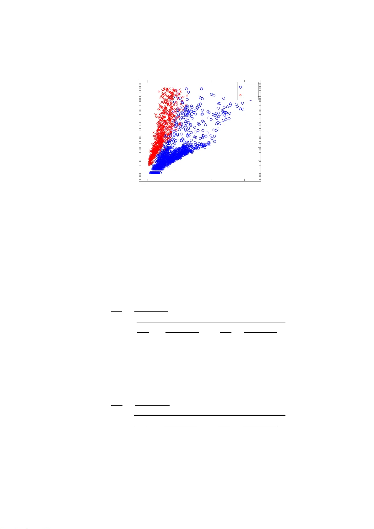
Solving Limited Memory Inﬂuence Diagrams ∗ Denis Deratani Mau´ a denis@idsia .ch Cassio P olp o de Campo s cassio@idsi a.ch Marco Zaﬀalon zaffalon@id sia.ch Istituto Dalle Molle di Studi sull’In telligenza Articiale (ID SIA) Galleria 2, Manno, 6928 - Switzerland Septem ber 23, 2018 Abstract W e present a new algorithm for exactly solving decision making prob- lems represented as inﬂuence diagrams. W e do not require th e usual assumptions of no forgetting and regularity; this allows us to solve prob- lems with simultaneo us decisions and limited information. The algorithm is empirical ly shown to outperform a state-of-the-art algorithm on ran- domly generated problems of up to 150 v ariables and 10 64 solutions. W e sho w th at the problem is NP-h ard even if t h e underlyin g graph structure of th e problem h as small treewidth and the v ariables take on a b oun d ed num ber of states, but that a fully p olynomial time approximation sc heme exists for these cases. Moreo v er, we sho w that the b ound on the num ber of states is a necessary condition for any eﬃcient app ro ximation sc heme. 1 In tro duction Inﬂuence diagrams [12] ar e graphical mo dels for utility-based decision making under uncertaint y . T raditionally , they are designed to r epresent and solve s itua- tions involving a single, non-forgetful decision mak er. Limited memory inﬂuence diagrams (herea fter LIMIDs) are gener alizations of inﬂuence diag r ams that al- low for multi-agent and limited information decision pro blems [16, 2 3]. 1 More precisely , LIMIDs relax the r e gularity and no for getting a ssumptions of inﬂuence diagrams, namely , that there is a complete temp oral order ing ov er the decision v ar iables, and that at any step any previo usly disclosed information is remem- ber ed a nd tak en into account to make a decisio n. These assumptions fail when decisions can b e made simultaneously (e.g., by no n- in teracting ag en ts), or when we wish to limit the decision histor y for co mputational reasons (e.g., to av oid an e xpo nen tial blow up in the s ize of policies ). ∗ A short version of this pap er has b een accept ed for presentat ion at NIPS 2011. 1 Historically , Ho w ard and Matheson [12] deﬁned inﬂuence diagrams as graphical r epresen- tations of g eneral decision sce narios, and referred to the sp ecial cases resp ecting r egularit y and no forgetting as de cision networks . The latter was then used b y Zhang et al. [23] to describe the general case. Here, we adopt the more recen t terminology of Lauritzen and Ni l sson [ 16]. 1 Solving a (limited memor y) inﬂuence diag ram refers to ﬁnding a combina- tion of lo cal decision rules (called a s trategy) that maximizes exp ected utility . This tas k has been empirically a nd theoretica lly shown to b e very hard [5]. In fact, w e show here that solving a LIMID is NP-complete if we admit only singly connected diagr ams with num ber of s ta tes p er v a riable no greater than three. In addition, w e show that an a lgorithm that pro duces prov ably go o d a pprox- imations within any ﬁxed factor is unlike to exist even for diagr ams with low treewidth, but that a fully poly nomial time approximation scheme exis ts if we further restr ict the v a r iables to take on a b ounded num ber of states. Under certain gr aph-structural conditions (which no forgetting and reg ular- it y imply), Lauritzen and Nilsson [1 6] show that LIMIDs can b e solved by a dynamic prog r amming pr o cedure with complex it y exp onential in the treewidth. How ev er, when these conditions ar e not met, their iterative algor ithm is only guaranteed to converge to a lo cal optimum. Recently , de Camp os and Ji [5] formulated the CR algo rithm tha t maps a LIMID into a cr edal net work [3] and then so lv es the co rresp onding marginal inference problem by mixed int eger lin- ear pr ogramming. By that, they were able to solve small problems exac tly and obtain go o d a pproximations for medium-sized problems. In this pap er, we sho w that (partial) com binations of lo cal decision rules can be partially ordered accor ding to the utility they induce, and that dominance of a partia l combin ation implies dominance of a ll (full) combinations that extend it. This grea tly reduces the sear ch space o f strateg ies. Using thes e re s ults we develop a genera lized v ariable elimina tion pro cedure that computes the optimal solution by propaga ting only non- do minated (partial) solutions. W e show ex- per imen tally that the algo rithm can enor mously s av e computational resources, and compute exact solutions for medium-sized pr o blems. In fact, the a lgorithm is or ders of mag nitude faster than the CR alg orithm on ra ndomly gener ated diagrams containing up to 15 0 v a riables a nd 1 0 64 strategies. The pap er is o rganized as follows. Section 2 formally de s crib es LIMIDs and presents new results a bo ut the complexity of solving a LIMID. In Sectio n 3, we pr e sen t a new algorithm for computing ex a ct globa l solutions and dis c uss its complexity . Section 4 contains the mo diﬁcations nece s sary to co n vert the algorithm into a fully p olynomia l time approximation scheme for diag rams of bo unded treewidth and num ber of states p er v ariable. The p erformance of the algo rithms is ev aluated in Section 5. Finally , Sections 6 a nd 7 contain related work and ﬁnal discussion. T o improv e r eadability , so me of the pr o o fs and s uppor ting results app ear in the app endix. 2 Limited Memory Inﬂ uence Diagrams In the for malism of (limited memor y) inﬂuence diagr a ms, the quantities and even ts o f int erest a r e represented b y three distinct types of v ariables or no des. 2 Chanc e variables repr esent even ts o n which the decisio n maker has no control, such as outcomes o f tes ts or co nsequences of actions. De ci sion variables re pr e- sent the options a decision maker might hav e. Finally , value variables repr esent additive pa rcels o f the utility asso ciated to a s tate of the world. The s et of all v ar ia bles considered relev a n t fo r a problem is denoted by U . E a ch v ariable 2 W e make no distinction b etw een a no de i n the graphical r epresen tation of a decision problem and i ts corresponding v ariable. 2 X in U ha s an as so ciated domain Ω X , which is the ﬁnite non-empty set of v alues X ca n take on. The elements of Ω X are called states . W e as sume the existence of the empty domain Ω ∅ , { λ } , which contains a single element λ which is not in any other domain. Decision and chance v aria ble s a re assumed to have domains diﬀerent fro m the empty domain, whereas v alue v ariables ar e alwa ys asso ciated to the empty domain. The do ma in Ω x of a set of v ariables x = { X 1 , . . . , X n } ⊆ U is given by the Car tes ian pro duct Ω X 1 × · · · × Ω X n of the v ar iable do ma ins. Thus, an element u ∈ Ω U deﬁnes a state of the world, that is, a realizatio n of a ll actions and ev ent s of interest. If x and y a r e se ts of v ar iables such that y ⊆ x ⊆ U , and x is an element o f the domain Ω x , we write x ↓ y to denote the pro jection of x onto the smaller domain Ω y , that is, x ↓ y ∈ Ω y contains only the co mponents of x that are compatible with the v ariables in y . By co n ven tion, x ↓∅ , λ . The cylindric al ex tension of y ∈ Ω y to Ω x is the set y ↑ x , { x ∈ Ω x : x ↓ y = y } . Often, we write X 1 · · · X n to denote the s et { X 1 , . . . , X n } and, if clear from the co n text, X to denote the sing leton { X } . Some op era tio ns ov er rea l-v alued functions need to b e deﬁned. Let f and g b e functions over domains Ω x and Ω y , res pectively . The pr oduct f g is deﬁned a s the function ov er doma in Ω x ∪ y such that ( f g )( w ) = f ( w ↓ x ) g ( w ↓ y ) for a n y w of its domain. Sum of functions is deﬁned analog ously: ( f + g )( w ) = f ( w ↓ x ) + g ( w ↓ y ). Notice tha t pr o duct and sum of functions are asso ciative and commut ative, and that pro duct distributes ov er sum, that is, f g = g f , f + g = g + f , and f ( g + h ) = f g + f h . If f is a function ov er Ω x , and y ⊆ U , the sum- mar ginal P y f returns a function over Ω x \ y such that for a n y element w of its domain w e hav e ( P y f )( w ) = P x ∈ w ↑ x f ( x ). Notice that if y ∩ x = ∅ , then P y f = f . Also, the sum-margina l op e r ation inherits commutativit y and asso ciativity from additio n of real num b ers, and hence P x ∪ y f = P x \ y P y f = P y \ x P x f . If { f y x } y ∈ Ω y is a set co n taining functions f y x with domain Ω x , one for each element o f Ω y , we wr ite f y x to denote the function that for all w ∈ Ω x ∪ y satisﬁes f y x ( w ) = f w ↓ y x ( w ↓ x ). F or instance, if X and Y a re tw o binary-v alued v ariables, and f y 1 X = ( f y 1 X ( x 1 ) , f y 1 X ( x 2 )) = (1 / 2 , 1 / 2) and f y 2 X = (0 , 1) t w o functions over { X } , then the function f Y X = ( f y 1 X ( x 1 ) , f y 1 X ( x 2 ) , f y 2 X ( x 1 ) , f y 2 X ( x 2 )) = (1 / 2 , 1 / 2 , 0 , 1). If clear from the c o n text, we w r ite 1 to deno te a function that r e tur ns one to all v alues in its doma in and 0 to denote a function that returns alwa ys zero. More g e ne r al, we wr ite k to denote a function that re tur ns alwa ys a co nstant real v a lue k . Hence, if f a nd g are functions ov er a do main Ω x and k is a real num ber, the express ions f ≥ g and f = k de no te that f ( x ) ≥ g ( x ) and f ( x ) = k , resp ectively , for all x ∈ Ω x . Finally , a n y function over a do main containing a single element is identiﬁed with the real n um b e r it returns. Let C deno te the s e t of chance v aria bles in U , D the set o f decision v ariables, and V the set of v alue v aria bles. The sets C , D and V fo r m a partition of U . A LIMID L consists of a direct acyclic g raph (DA G) ov er the set of v ar iables U a nnotated with v aria ble t ypes (decisio n, chance and v alue), together with a collection of (conditional) pr obability mass functions (o ne for eac h chance v alue) and utility functions (one for ea c h v alue v ariable). 3 The v a lue nodes in the g raph hav e no c hildren. The precise meanings of the a rcs in L v ar y acco rding to the t yp e of no de to which they p oint . Arcs entering chance and v alue no des deno te sto chastic a nd functional dependency , r espe ctiv ely; ar cs entering decision no des 3 When no confusion arises, we wr ite L to r ef er both to the LIMID and to its directed graph. 3 D 1 D 2 D n X 0 X 1 X 2 · · · X n R Figure 1: LIMID o f the problem in the Exa mple 1. describ e information aw areness or r elev ance at the time the decision is made. If X is a no de in L , we denote b y pa X the set of par ent s of X , that is, the set of node s o f L fr om whic h there is a n arc p ointing to X . Similarly , we let c h X denote the s et of children o f X (i.e., no des to which there is an arc from X ), and fa X , pa X ∪ { X } denote its family . The descenda n ts of X are all no des to which there is a directed path from X in L . Each chance v ariable C in C has an a sso ciated set { p π C : π ∈ Ω pa C } o f (conditional) proba bilit y mass functions p π C quantifying the decision maker’s b eliefs ab out states x ∈ Ω C conditional on a state π o f its parents (if C has no parents, it has a single probability mass function assigned). W e a ssume any chance v ar iable X ∈ C to be sto chastically independent fro m its non-desc endant non-parents given its parents. Each v a lue v ar iable V ∈ V is a sso ciated with a rea l-v alued utility function u V ov er Ω pa V , which quantiﬁes the (additive) contribution of the sta tes of its par en ts to the ov erall utility . Thus, the ov erall utilit y of a state x ∈ Ω C ∪D is given by the sum of utility functions P V ∈V u V ( x ↓ pa V ). F or any decisio n v a riable D ∈ D , a p olicy δ D sp eciﬁes an a ction for each po ssible state co nﬁguration of its parents, that is , δ D : Ω pa D → Ω D . If D has no pa rents, then δ D is a function from the empty domain to Ω D , and therefore constitutes a choice of x ∈ Ω D . The s et o f a ll p olicies δ D for a v a riable D is denoted by ∆ D . The fo llowing a rtiﬁcial examples help to illustra te the use o f LIMIDs for mo deling decision-making problems under uncer taint y inv olving multiple deci- sion makers with limited infor mation. Example 1. Consider a game wher e e ach of the n p articip ants has to de cide b etwe en adding a b al l to an urn or r emoving a b al l fr om it, without knowing neither t he state of the urn nor the other p articip ants’ de cisions. If a p articip ant de cides for r emoval when t he urn is empty then two b al ls ar e put. If the u rn alr e ady c ontains t wo b al ls, a de cision of adding a b al l is ignor e d. The go al is to ﬁnish the se quenc e of n de cisions with no b al ls in the urn. T o avoid inter c ommunic atio n, the p articip ant s ar e kept in sep ar ate r o oms, and they ar e aske d for a de cision in some pr e- determine d or dering un known t o t hem. Figur e 1 depicts the gr ap h structur e of a LIMID mo deling the pr oblem. As usual, we gr aphic al ly r epr esent de cision, chanc e, and value variables by squar es, ovals and diamonds, r esp e ctivel y. The n o des D 1 , . . . , D n r epr esent the de cisions available to e ach of the p articip ants in the given or dering. Each chanc e no de X i r epr esents the nu m b er of b al ls in t he u rn after i de cisions have b e en made ( 0,1, or 2), and is t her efor e asso ciate d to a deterministic function ( X 0 mo dels t he initial state of the urn). The value no de R has an asso ciate d utility function that re turns 1 if the state of X n is the element c orr esp onding to an empty u rn, and zer o otherwise. F or any D i , a p olicy δ D i c orr esp onds to a ﬁxe d de cision of adding or r emoving a b al l for the i th p articip ant. 4 D 1 D 2 · · · D n X 0 X 1 X 2 · · · X n R Figure 2: LIMID o f the problem in the Exa mple 2. Example 2. Consider a slightly mo diﬁe d version of the game in Example 1 , wher e e ach p artici p ant is informe d of the pr evious de cision. Also, the initial state of the urn is disclose d to the ﬁrst p articip ant (so the ﬁrst p articip ant is awar e he/she is t he ﬁrst to make a de cision, but al l the other r emain ignor ant ab out their p osi tions in the se quenc e). Figur e 2 depicts t he gr ap h st ructur e of a LIMID mo deling the pr oblem. Notic e the extr a ar cs fr om D i to D i − 1 , i = 1 , . . . , n − 1 , r epr esenting that t he de cision made by the ( i − 1) - th p articip ant is known to the i -th p articip ant, and the ar c X 0 → D 1 indic ating t he known state of the urn to the ﬁrst p articip ant to make a de cision. The p olicy δ D 1 pr escrib es a de cision (to add or r emove a b al l) for the ﬁrst p articip ant for e ach p ossibl e initial s tate of the urn (empty, one b al l or t wo b al ls). Similarly, for i = 2 , . . . , n , a p olicy δ D i sp e ciﬁes whether t he i -th p articip ant s hould de cide to add a b al l dep ending on the ( i − 1 ) -th p articip ant’s de cision. F or example, if δ D 2 = ( δ D 2 ( add ) , δ D 2 ( r emove )) denotes the p olicy of the se c ond p articip ant (which is a function of the ﬁrst p ar- ticip ant’s de cisio n), then p olicy δ D 2 = ( r emove , add ) pr escrib es that the se c ond p articip ant should r emove a b all when the ﬁrst p articip ant de cid es for addition, and otherwise add a b al l. The four p ossible p oli cies for t he se c ond p articip ant ar e ∆ D 2 = { ( add , r emove ) , ( add , add ) , ( r emove , add ) , ( r emove , r emove ) } . Let ∆ , × D ∈D ∆ D denote the space of p ossible combination o f p o licies. An element s = ( δ D ) D ∈D ∈ ∆ is sa id to b e a str ate gy for L . Given a p olicy δ D and a state π ∈ Ω pa D , let p π D denote a proba bility ma ss function for D conditional on pa D = π such that p π D ( x ) = 1 if x = δ D ( π ) and p π D ( x ) = 0 otherwise. Hence, there is a one-to-o ne cor resp ondence b etw een functions p pa D D and p olicies δ D ∈ ∆ D , a nd s pecifying a p o licy δ D is equiv a le n t to sp ecifying p pa D D . W e deno te the set o f all functions p pa D D obtained in this way by P D . A strategy s induces a joint pro babilit y mass function over the v ariables in C ∪ D by p s , Y C ∈C p pa C C Y D ∈D p pa D D , (1) and ha s an asso ciated exp ected utilit y given by E s [ L ] , X x ∈ Ω C∪D p s ( x ) X V ∈V u V ( x ↓ pa V ) (2) = X C ∪D p s X V ∈V u V . (3) Notice that the tw o sums in Eq. (3) hav e diﬀerent se man tics. The outer (left- most) s um denotes the sum-mar ginal of the set of v ar iables C ∪ D , wherea s the inner (rightmost) denotes the o verall utility function over S V ∈V pa V that res ults from the sum of functions u V . 5 The tr e ewidth of a gra ph mea sures its resemblance to a tr ee and is given by the num ber o f vertices in the larg est clique of the corresp onding triangulated moral g raph minus one [1]. Given a LIMID L o f tr eewidth ω , we can ev aluate the exp ected utility of any strateg y s in time and spa ce at most exp onential in ω . Hence, if ω is b ounded by a consta nt, obtaining E s [ L ] takes p olynomial time: Prop osition 3. Given a LIMID L with b ounde d tr e ewidth and a str ate gy s , E s [ L ] c an b e c ompute d in p olynomia l time. Pr o of. Given a str a tegy , the LIMID can b e mapp ed into a LIMID with no decision no des in p olyno mial time by replacing each decis ion no de D by a chance no de with as so ciated probability table p pa D D . The bo unded treewidth implies that the num b er of pare n ts of any decision no de is b ounded, and then enco ding p pa D D takes time p olynomial in the n um be r of element s in fa D (an input of the LIMID). Then the L VE algor ithm in Section 3 can b e employ ed, which runs in po lynomial time since there ar e no decisions in the input (therefor e a ll sets ar e singletons) and the treewidth is b ounded. 4 The primary task o f a LIMID is to ﬁnd a strategy s ∗ with maximal exp ected utilit y , tha t is , to ﬁnd s ∗ ∈ ∆ such that E s [ L ] ≤ E s ∗ [ L ] for all s. (4) The v alue E s ∗ [ L ] is called the maximum exp e cte d u tility of L and it is denoted b y MEU[ L ]. F or most real problems, enum erating a ll the strateg ies is prohibitively costly . In fa c t, computing the MEU in bo unded treewidth diagrams is NP- complete [5], and, as the following result implies , it r emains NP-c omplete in even simpler LIMIDs. Theorem 4 . Given a singly c onne ct e d 5 LIMID with tr e ewidth e qual to 2, and with variables having at most thr e e states, de ciding whether ther e is a s t r ate gy with ex p e cte d utility gr e ater t han a given k is NP-c omplete. The pr oo f, based on a re ductio n from the par tition problem, is given in the app endix. Notice that the s imple LIMIDs of E x amples 1 and 2 (depicted in Figures 1 a nd 2, resp ectively) meet the pr econditions o f Theor em 4, and are in general mo st unlikely to b e eﬃciently solv a ble for any s uﬃcie ntly lar ge n (in fact, the ha r dness is shown b y a reduction o f an NP-complete problem to the problem of deciding whether the MEU o f the LIMID in Exa mple 1 is gr eater than a given threshold). The complexity o f solving a LIMID c a n b e reduced by removing no des and arcs that are irr elev ant to the c omputation of the maximum exp ected utility . A chance or decision no de is called b arr en if it has no children. Barren no des hav e no inﬂuence o n a n y v alue no de and thus no impact on the ME U [8]. More irrelev ances can b e found by the concept of d -separ ation [19], which w e succinctly state in the following par agraph. A tr ail in L is a sequence of no des s uc h that a n y tw o conse cutiv e no des are connected by an a r c. Notice that a trail do es not need to “fo llow” the direction 4 See also Koller and F r iedman [ 15] f or a sl igh tly s impler v ari able eli mination algori thm that computes ﬁxed-strategy s olutions of b ounded treewidth diagrams in p olynomial time. 5 A directed graph is singly connected i f the underlying (undirected) graph con tains no cycles. 6 D 1 D 2 · · · D n X 0 X 1 X 2 · · · X n R Figure 3: LIMID o f the problem in the Exa mple 5. D 1 D 2 · · · D n X 0 X 1 X 2 · · · X n R Figure 4 : LIMID of the pr oblem in the E xample 5 after the remov al of nonreq- uisite arcs. of the a rcs. A trail X , Z, Y is said to be active with resp ect to a set of v ar iables w e ither if X a nd Y ar e b oth parents of Z and Z o r any of its desce nda n ts a r e in w , or if at least one of X a nd Y is not a parent o f Z and Z is no t in w . A trail is blo cke d by a set o f v ariables w if it contains a triple of consecutive no des which is no t active with resp ect to w . Two s ets of no des x and y are d -sep ar ate d by a s et o f no des w if all trails from a no de X in x to a no de Y in y ar e blo ck ed by w . Intuitiv ely , if X and Y are d -separa ted by w , then X and Y are ir relev ant to ea ch other once we know the state of the v ariables in w . A par en t no de X of a decision no de D is nonr e qu isite (to D ) if it is d - separated from all the v a lue no des that are descenda nt of D given all the re- maining parents and D . The a rc from X to D is then sa id to b e a nonr e quisite ar c . Likewise barren no des, nonrequisite ar cs can b e r emov ed without aﬀecting the MEU [8, 16], and by doing so a no de may bec o me barren. W e say that a LIMID is minimal if it contains no no nrequisite arcs and no barren no des. Given a LIMID w e can obtain its cor r esp onding minimal dia gram in p olynomial time by rep eatedly removing nonrequisite arcs and barre n no des [13, 1 6]. F or the rest of this pap er, we ass ume LIMIDs to b e minimal. The following example illustrates the co nc e pts o f d -separatio n and nonreq - uisite arcs. Example 5. Consider a mo diﬁe d version of t he multiplayer game in Example 2, wher e in additio n to the pr evi ous p articip ant’s de cision also t he curr ent st ate of the urn is disclose d to a p articip ant b efor e he/she makes a de cision. The gr aph structur e of a LIMID r epr esenting t his pr oblem is depicte d in Figur e 3. N otic e the ar cs X i − 1 → D i , for i = 1 , . . . , n − 1 , r epr esenting t he known state of the urn to e ach p articip ant. Consider the ar c D 1 → D 2 . Al l tr ails c onne cting D 1 and R ar e blo cke d by fa D 2 \ { D 1 } = { D 2 , X 1 } . Ther efor e D 1 is a nonr e qu isite no de for D 2 and the ar c D 1 → D 2 c an b e r emove d without altering the MEU. In fact, al l ar cs D i − 1 → D i , for i = 1 , . . . , n , ar e nonr e quisite and c an b e safely r emove d. On the other hand, X 0 is a r e quisite no de for D 1 b e c ause, for instanc e, the tra il X 0 , X 1 , . . . , X n , R is active given the set fa D 1 \ { X 0 } = { D 1 } . Intuitively, the information pr ovide d by the ar cs D i − 1 → D i (i.e., the pr evious p artici p ant’s de cision) do es not help in making a de cision onc e the curr ent state X i − 1 of the 7 urn is known. Figur e 4 depicts a minimal version of the diag r am in Figur e 3 . Under the usual ass umptions of complexity theory , when a proble m is NP- hard to so lve the bes t av aila ble options are (i) trying to devise an algo rithm that runs eﬃcient ly on many instances but has exp onential worst-case complexit y , o r (ii) trying to develop an appr oximation algor ithm that for all instances pr ovides in p olyno mial time a so lution that is prov ably within a certain r ange o f the optimal solution. In Section 3, we take option (i), and present an algorithm that eﬃciently c o mputes optimal solutions for many LIMIDs, but r uns in ex p onential time for many others. Given ǫ > 0 , a n ǫ -approximation algorithm (for solving a LIMID) obtains a strategy s s uch that (1 + ǫ ) E s [ L ] ≥ MEU[ L ]. As the following result indica tes, alternative (ii) is mos t likely unfeasible, even if w e conside r only diagrams of bo unded treewidth. Theorem 6. Given a singly c onne cte d LIMID L with b ounde d tr e ewidth, (un less P=NP) ther e is n o p olynomial time ǫ -appr oximation algorithm, for any 0 < ǫ < 2 θ − 1 , wher e θ is the numb er of n umeric al p ar ameters (pr ob abilities and utilities) r e quir e d t o sp e cify L . W e defer the pr o o f to the a pp endix. How ev er, we show in Section 4 that, diﬀerently from the ge neral case, there are LIMIDs, namely , thos e with bo unded treewidth and num b er of sta tes per v ariable, for which a p olynomial time ǫ - approximation algo rithm exists. Let L be a LIMID and let k and K denote, resp ectively , the smallest and the greatest utilities asso ciated to any of the v alue v ar iables, that is, for all V ∈ V we hav e that k ≤ u V ≤ K , and there are V and V ′ such that u V ( x ) = k and u V ′ ( x ′ ) = K for some x ∈ Ω pa V and x ′ ∈ Ω pa V ′ . Assume k < K (otherwise the MEU is triv ial), and let L ′ be the LIMID obtained from L b y setting each utilit y function u V asso ciated to a v alue no de V to u ′ V = ( u V − k ) / ( K − k ). No te that by design ea c h function u ′ V takes v alues on [0 , 1]. The fo llowing well-known result allows us to fo cus on sca led utility functions. Prop osition 7. F or any str ate gy s , E s [ L ] = ( K − k ) E s [ L ′ ] + k |V | . Pr o of. The case of a single v alue no de has b een s hown by Co op er [2] and Shach ter and Peot [21]. The extens io n to multiple v alue no des is straightfor- ward. F or a n y str ategy s we have tha t E s [ L ′ ] = X C ∪D p s X V ∈V u ′ V = X C ∪D p s X V ∈V u V − k K − k = 1 K − k X C ∪D p s − k |V | + X V ∈V u V ! = 1 K − k − k |V | X C ∪D p s + X C ∪D p s X V ∈V u V ! which, since p s is a probability distribution on C ∪ D , equals 1 K − k (E s [ L ] − k |V | ) . Hence, the result follows. 8 In the rest of the pap e r we consider only LIMIDs with utilities taking v alues in some subset of the r eal interv al [0 , 1 ], which due to P r op osition 7 do es not incur any loss of gener ality . 3 Solving LIMIDs Exactly The basic ingr edient s o f o ur a lg orithmic framework for represe nting a nd ha n- dling information in LIMIDs are the so called valuations , which enco de informa- tion (probabilities , utilities a nd p olicies) ab out the elements of a do main. Each v aluatio n is asso ciated to a subset of the v ar iables in U , called its sc op e . Mor e concretely , a v aluation φ with scop e x is a pair ( p, u ) of b ounded nonnegative real-v alued functions p and u over the domain Ω x ; we refer to p a nd u as the probability and utilit y part, res pectively , o f φ . Often, we write φ x to make explicit the scop e x of a v a luation φ . F or any x ⊆ U , we denoted the set o f all p ossible v a luations with scop e x by Φ x . The set o f all p oss ible v aluations is th us given by Φ , S x ⊆U Φ x . The s e t Φ is clo sed under tw o basic op era tio ns of c ombination a nd mar ginali zation . Combination represe n ts the agg regation o f information and is deﬁned as follows. Deﬁnition 8. If φ = ( p, u ) and ψ = ( q , v ) ar e valuations with sc op es x and y , r esp e ctively, its c ombination φ ⊗ ψ is the valuation ( pq , pv + q u ) with sc op e x ∪ y . Marginaliza tion, on the o ther ha nd, acts by coarsening information: Deﬁnition 9. If φ = ( p, u ) is a valuation with sc op e x , and y is a set of variables such that y ⊆ x , t he mar ginal φ ↓ y is the valuation ( P x \ y p, P x \ y u ) with sc op e y . In this c ase, we say that z , x \ y has b e en eliminated fr om φ , which we denote by φ − z . Notice that o ur deﬁnitions of combination and ma rginalization diﬀer from previous works on LIMIDs (e.g., [16]), which us ually r equire a divis ion o f the utilit y pa r t by the probability part. T he re mo v al of division turns out to b e a n impo rtant feature when we discuss max ima lit y o f v aluations la ter o n. In terms of computational complexity , combining tw o v a luations φ and ψ with scop es x and y , resp ectively , requir es 3 | Ω x ∪ y | mult iplications and | Ω x ∪ y | additions of num bers; computing φ ↓ y , wher e y ⊆ x , cos ts | Ω x ∪ y | op erations of addition. In other words, the cos t of co m bining or marg inalizing a v aluation is exp onent ial in the cardinality of its scop e (and linear in the cardinality of its domain). Hence, we wish to work with v aluations whose sco pe is as small as po ssible. The following result s hows that our framework resp ects the necessar y conditions for computing eﬃciently with v alua tions (in the sense of keeping the scop e o f v aluatio ns o bta ined from c om binations and marginaliza tions of other v aluatio ns minimal). Prop osition 10 . The system (Φ , U , ⊗ , ↓ ) satisﬁes t he fol lowing t hr e e axioms of a ( we ak) lab eled v alua tion alg ebra [14, 22]. (A1) Combination is c ommutative and asso ciative, that is, for any φ 1 , φ 2 , φ 3 ∈ Φ we have that φ 1 ⊗ φ 2 = φ 2 ⊗ φ 1 , φ 1 ⊗ ( φ 2 ⊗ φ 3 ) = ( φ 1 ⊗ φ 2 ) ⊗ φ 3 . 9 (A2) Mar ginalization is tr ansitive, that is, for φ z ∈ Φ z and y ⊆ x ⊆ z we have that ( φ ↓ x z ) ↓ y = φ ↓ y z . (A3) Mar ginalization distributes over c ombination, that is, for φ x ∈ Φ x , φ y ∈ Φ y and x ⊆ z ⊆ x ∪ y we have that ( φ x ⊗ φ y ) ↓ z = φ x ⊗ φ ↓ y ∩ z y . Pr o of. (A1) follows directly from commutativit y , asso ciativity and distributivity of pro duct and sum of rea l-v alued functions, and (A2) follows directly from commutativit y o f the sum-marg inal op eration. T o show (A3), consider any tw o v aluatio ns ( p, u ) and ( q , v ) with sco pes x and y , resp ectively , and a set z such that x ⊆ z ⊆ x ∪ y . B y deﬁnition of ⊗ and ↓ , we hav e that [( p, u ) ⊗ ( q , v )] ↓ z =   X x ∪ y \ z pq , X x ∪ y \ z ( pv + q u )   . Since x ∪ y \ z = y \ z , and p a nd u ar e functions over Ω x , it follows that   X x ∪ y \ z pq , X x ∪ y \ z ( pv + q u )   =   p X y \ z q , p X y \ z v + u X y \ z q   = ( p, u ) ⊗   X y \ z q , X y \ z v   , which equals ( p, y ) ⊗ ( q , v ) ↓ y ∩ z . The following is a dir ect consequence of (A3) that is required to pr ov e the correctnes s of the v a riable elimination pro cedure. Lemma 11. If φ x ∈ Φ x , φ y ∈ Φ y , z ⊆ y and z ∩ x = ∅ , t hen ( φ x ⊗ φ y ) − z = φ x ⊗ φ − z y . Pr o of. Let w = x ∪ y \ z . Since x ∩ z = ∅ , it follows that x ⊆ w ⊆ x ∪ y . Hence, by deﬁnition of elimination and (A3), we have that ( φ x ⊗ φ y ) − z = ( φ x ⊗ φ y ) ↓ w = φ x ⊗ φ ↓ y ∩ w y . But y ∩ w = y \ z . Th us, φ ↓ y ∩ w y = φ − z y . The following re sult shows how v aluations ca n b e used to c ompute ex p ected utilities for a given strateg y . Prop osition 12. Given a LIMID L and a str ate gy s = ( δ D ) D ∈D ∈ ∆ , let φ s , " O C ∈C  p pa C C , 0  # ⊗ " O D ∈D  p pa D D , 0  # ⊗ " O V ∈V (1 , u V ) # , (5) wher e, for e ach D , p pa D D is the function in P D asso ciate d with p oli cy δ D . Then φ ↓∅ s e quals (1 , E s [ L ]) . 10 Pr o of. Let p and u denote the pr o bability and utilit y part, r esp ectively , of φ ↓∅ s . By deﬁnition of c om bination, we hav e that φ s = ( p s , p s P V ∈V u V ), where p s = Q X ∈ C ∪D p pa X X as in (1). Since p s is a pr o bability distribution over C ∪ D , it follows that p = P x ∈ Ω C∪D p s ( x ) = 1. Finally , u = P C ∪D p s P V ∈V u V , which equals E s [ L ] by (3). Hence, given a strategy we can use a v aria ble elimination pro cedur e 6 to compute its exp ected utility in time p olyno mial in the largest domain of a v a ri- able but exp onential in the width o f the elimination ordering [e.g ., 15, Section 23.4.3]. 7 How ev er, computing the MEU in this wa y is unfeasible for realistic di- agrams due to the la rge num ber of str a tegies that would nee d to b e enumerated. F or example, a simple L IMID consisting of a decision v aria ble with four chance no des a s parents and one v alue no de as child contains 10 3 4 = 10 81 strategies in ∆, if the decision v ariable ha s 10 states and each par en t has 3 sta tes. In or der to avoid having to cons ider a ll p ossible s trategies, w e deﬁne a partial order (i.e., a reﬂexive, antisymmetric and transitive relation) over Φ as follows. Deﬁnition 13. F or any t wo valuations φ = ( p, u ) and ψ = ( q , v ) in Φ , we say that ψ dominates φ (c onversely, we say that φ is dominated by ψ ), and we write φ ≤ ψ , if φ and ψ have e qual sc op e, p ≤ q , and u ≤ v . If φ and ψ hav e scop e x , deciding whether ψ dominates φ costs at most 2 | Ω x | op eratio ns of compa rison of num bers . The following result shows that the algebra of v alua tio ns is monotonic w ith resp e ct to dominance. Prop osition 14. The system (Φ , U , ⊗ , ↓ , ≤ ) satisﬁes the fol lowing two addi- tional axioms of an ordered v alua tion alg ebra [11]. (A4) Combination is monotonic with r esp e ct to dominanc e, that is, if φ x ≤ ψ x and φ y ≤ ψ y then ( φ x ⊗ φ y ) ≤ ( ψ x ⊗ ψ y ) . (A5) Mar ginalization is monotonic with r esp e ct to dominanc e, t hat is, if φ x ≤ ψ x then φ ↓ y x ≤ ψ ↓ y x . Pr o of. (A4). Consider tw o v aluations ( p x , u x ) and ( q x , v x ) with scop e x such that ( p x , u x ) ≤ ( q x , v x ), a nd tw o v a luations ( p y , u y ) and ( q y , v y ) with sco pe y satisfying ( p y , u y ) ≤ ( q y , v y ). By deﬁnition o f ≤ , we hav e tha t p x ≤ q x , u x ≤ v x , p y ≤ q y and u y ≤ v y . Since all functions are nonnegative, it follows that p x p y ≤ q x q y , p x u y ≤ q x v y and p y u x ≤ q y v x . Hence, ( p x , u x ) ⊗ ( p y , u y ) = ( p x p y , p x u y + p y u x ) ≤ ( q x q y , q x v y + q y v x ) = ( q x , v x ) ⊗ ( q y , v y ). (A5). Let y be a subset o f x . It follows from monotonicity o f ≤ with r esp ect to addition of re a l nu mbers that ( p x , u x ) ↓ y =   X x \ y p x , X x \ y u x   ≤   X x \ y q x , X x \ y v x   = ( q x , v x ) ↓ y . Hence, the result follows. 6 V ariable elimination algorithms are also kno wn in the li terature as fusion algorithms [22] and buc k et elimination [6]. 7 The width of an elim i nation orderi ng i s the treewidth of the tree decomp osition it induces and can be computed in tim e p olynomial in the num ber of v ari ables. It also equals the maximum cardinali t y of the scop e of a v aluation in the v ariable elimination procedure minus one. 11 The a lgorithm we devise later on op erates on sets of or dered v aluations. Deﬁnition 15. Given a ﬁn ite set of valuations Ψ ⊆ Φ , we say t hat φ ∈ Ψ is maximal if for al l ψ ∈ Ψ su ch that φ ≤ ψ it holds t hat ψ ≤ φ . The op er ator max re turns the set max(Ψ) of maximal valuations of Ψ . If Ψ x is a set with m v alua tio ns with sc o pe x , max(Ψ x ) can b e obtained by m 2 compariso ns φ ≤ ψ , where ( φ, ψ ) ∈ Ψ x × Ψ x . W e extend co m bination and marginaliza tion to sets of v aluatio ns as follows. Deﬁnition 1 6 . If Ψ x and Ψ y ar e any two sets of valuations in Φ , Ψ x ⊗ Ψ y , { φ x ⊗ φ y : φ x ∈ Ψ x , φ y ∈ Ψ y } denotes the set obtaine d fr om al l c ombinations of a valuation in Ψ x and a val- uation in Ψ y . Deﬁnition 1 7 . If Ψ x ⊆ Φ x is a set of valuations with sc op e x and y ⊆ x , Ψ ↓ y x , { φ ↓ y x : φ x ∈ Ψ x } denote the set of valuations obtaine d by element - wise mar ginalization of valua- tions to y . It can b e chec k ed that sets of v a luations with combination a nd ma rginal- ization deﬁned element-wise satisfy axioms (A1 )– (A3), a nd therefore form a v aluatio n algebr a . Hence, Lemma 1 1 applies also for sets of v alua tions with marginaliza tion and combination deﬁned as a b ove. Lemma 18. If Ψ x ⊆ Φ x and Ψ y ⊆ Φ y ar e t wo sets of valuations with s c op e x and y , r esp e ctively, and z is a set of variables such that z ⊆ y and z ∩ x = ∅ , then (Ψ x ⊗ Ψ y ) − z = Ψ x ⊗ Ψ − z y . Pr o of. The result follows fro m element-wise a pplica tion o f Lemma 11 to ( φ x ⊗ φ y ) − z ∈ (Ψ x ⊗ Ψ y ) − z . W e are now r eady to describ e the L VE algo ri thm , whic h solves ar bitrary LIMIDs exa ctly . Consider a LIMID L , and an order ing X 1 < · · · < X n ov er the v a riables in C ∪ D . The algo rithm is initialized by ge ne r ating o ne set of v aluatio ns for ea c h v ariable X in U a s follows. Initialization: Let V 0 be initially the empty set. 1. F o r ea ch chance v ariable X ∈ C , a dd a single to n Ψ X , { ( p pa X X , 0) } to V 0 . 2. F o r e ach de c ision v ariable X ∈ D , add a set of v a luations Ψ X , { ( p pa X X , 0) : p pa X X ∈ P X } to V 0 . 3. F o r ea ch v alue v ariable X ∈ V , add a singleton Ψ X , { (1 , u X ) } to V 0 . Once V 0 has b een initialized with a s et o f v aluatio ns for each v aria ble in the diagram, we recursively eliminate a v ariable X i in C ∪ D in the given ordering and r emov e any non-maximal v aluation: Propagation: F or i = 1 , . . . , n do: 12 1. Let B i = ∅ . Remov e from V i − 1 all s e ts whose v a luations contain X i in their s cop e and add them to B i . 2. Compute Ψ i , max([ N Ψ ∈B i Ψ] − X i ). 3. Set V i , V i − 1 ∪ { Ψ i } . T ermination: Fina lly , the alg o rithm outputs the utility part of the single maximal v aluation in the set N Ψ ∈V n Ψ, tha t is, the algorithm re tur ns the r e al nu mber u s uc h that ( p, u ) ∈ max( N Ψ ∈V n Ψ). u is a r eal num ber b ecause the v aluatio ns in N Ψ ∈V n Ψ have empt y scop e and thus b oth their pr o bability a nd utilit y parts can b e identiﬁed with rea l num ber s . The elimina tio n ordering X 1 < · · · < X n can be determined using the sta n- dard heuristics for v ariable elimina tio n in B ay esian net works such as minimizing the num b er of ﬁll- ins or the car dinalit y o f the domain of the neighbor set [13, 15]. Diﬀerent ly from other mes sage-pas s ing algorithms that obtain appr oximate solutions to LIMIDs by (rep eatedly) pro pagating a single v a luation (e.g ., the SPU alg orithm [16]), the L VE alg orithm computes exact solutions by pr opagat- ing many maximal v alua tions that c orresp ond to par tial com binations of loca l decision rules. The eﬃciency of the algor ithm in handling the pro pa gation of several v aluations derives from the ea rly r emov a l of v aluations p erformed by the max op eration in the pro pagation step. Consider the set Ψ L , { φ s : s ∈ ∆ } , where each φ s is given by (5). It is no t diﬃcult to see that Ψ L = " O C ∈C  p pa C C , 0  # ⊗ " O D ∈D  p pa D D , 0  : p pa D D ∈ P D  # ⊗ " O V ∈V { (1 , u V ) } # = O Ψ X ∈V 0 Ψ X . Hence, by Prop osition 12 we hav e that each φ ↓∅ s in Ψ ↓∅ L is a v alua tio n with prob- ability part o ne a nd utility part equal to the exp ected utility of some strategy in ∆. Since the r elation ≤ induces a strict (linea r) orde r over Ψ ↓∅ L , the MEU of the diagram equals the utility par t o f the (sing le) v aluation in max(Ψ ↓∅ L ). The v ari- able e limina tion pro cedure in the propagatio n step is resp onsible for obtaining max( N Ψ ∈V n Ψ) = max (Ψ ↓∅ L ) more e ﬃcien tly by distributing ma x and ↓ over N Ψ X ∈V 0 Ψ X , which allows for a signiﬁcant reduction in the cardinalities of sets and scop es of v aluations pro duced. The following result states the correctness of the algo rithm. Theorem 19. Given a LIMID L , L V E outputs MEU[ L ] . The pr oo f, which r equires so me technicalities, is in the app endix. 3.1 Complexit y Analysis Assume that decis ion no des are par en tless. W e will show in Se c tio n 3.4 later on that w e can tra nsform any given LIMID into an equiv alen t mo del in whic h decision nodes have no pa r ent s. Parentless decisions allows us to av oid having to dea l with sets whose cardina lit y is exp onential in the num ber o f parents. 13 The time complex it y of the algor ithm is given by the cost o f c r eating the sets of v a luations in the initialization step plus the ov erall cos t o f the combination and marg inalization op erations p erfor med during the propa g ation step. Re- garding the initia lization step, the lo ops for chance and v alue v ar ia bles genera te singletons, and thus take time linea r in the input. Since decision no des hav e no parents, ther e are ρ D , | Ω D | p olicies in ∆ D (whic h co incides with the n um b e r of functions in P D ) for each decision v ariable D . Ther e is one v alua tion in the corres p onding set Ψ D added to V 0 for every p olicy in ∆ D . Let ρ , max D ∈D ρ D be the ca rdinality of the larges t p olicy set. Then the initialization loo p for de- cision v ariables ta k es O ( |D | ρ ) time, which is p olynomia l in the input. L e t us now a na lyze the propag ation step. As with any v ariable elimination pr o cedure, the r unning time o f pro pagating (sets of ) v alua tions is exp onential in the width of the elimina tion or dering, which is in the b est case g iven by the treewidth of the diag ram. Cons ider the case o f an elimination order ing with b ounded width ω , and a diagram with b ounded num b er of states p er v ariable κ . Then the cost of ea c h co m bination o r ma rginalization is b ounded by a constant, and the complexity depe nds only on the num b er of o p era tions perfo rmed. Moreover, we hav e in this case that ρ ≤ κ . Let ν denote the cardinality of the lar gest set Ψ i , for i = 1 , . . . , n . Thus, c omputing Ψ i requires at most ν |U |− 1 op erations of combination (beca us e that is the maximum num ber o f sets that we might need to co m bine to c o mpute N Ψ ∈B i Ψ in the pr o pagation step) and ν op erations of marginaliza tion. In the worst case, ν is equal to ρ |D | ≤ O ( κ |D | ), that is , all sets asso ciated to decision v ariables hav e b een co m bined without discar ding any v al- uation. Hence, the worst-case complexity of the propag a tion step is exp onential in the n um ber of decision v a r iables, even if the width of the elimina tion ordering and the num ber o f states p er v aria ble a re b o unded. Note how ever that this is a very pessimis tic scenar io a nd, on av erage, the remov al of non-maximal elements greatly reduces the complexity , as the exp eriments in Section 5 show. 3.2 Strategy Selection Most likely , one is not only interested in the ma xim um exp ected utilit y of a LIMID but also in a n optimum course of ac tio n for every po ssible scenar io , that is, in a n optimal strateg y that obtains the MEU. L VE can b e easily mo diﬁed to provide an o ptimal strategy by stor ing a t ea ch step the p olicies as so ciated to non-domina ted v aluations as follows. F or each v aluation crea ted in the ini- tialization step asso ciate a list which is empty unles s the v aluation refer s to a po licy of a decis ion v ariable, in which case the list contains the asso ciated p olicy . Now, any v aluation φ i ∈ Ψ i factorizes as ( ψ 1 ⊗ · · · ⊗ ψ |B i | ) − X i , where each ψ j is a n element of a diﬀer e n t set Ψ in B i . F o r i = 1 , each ψ j is a sso ciated to a list. Assign a list to each φ 1 which equa ls the concatena tion of the lists of its factors ψ j . Thus, the list cont ains a choice o f p olicies for all decis io n v ariables D s uc h that X 1 ∈ fa D . F or ea ch i , a s so ciate a list to each φ i ∈ Ψ i which equals the concatenation of lists of its factors. An optimal strategy s ∗ is thus easily obtained fro m the list as so ciated to φ n ∈ max( N Ψ ∈V n Ψ). The handling o f lists can b e implement ed by s imple p ointers to v aluations in sets in V 0 , and there fo re the asymptotic complexity of the a lgorithm is unaltered. 14 3.3 Rev erse T op ological Ordering The v aluations us e d by L VE s pecify twice a s many num bers as the car dinality of the domain of their a sso ciated scop e. It is p oss ible to decrea se b y a factor of t wo the num b er of numerical par ameters p er v a luation the algor ithm nee ds to handle by constra ining the elimination o f v ariables to follow a reverse top ologic al ordering in the dia g ram, tha t is, by r equiring each v ar iable to b e pro cesse d only after all its descendants have b een pro cessed. As the following result sho ws, any reverse top ologica l ordering pro duces v aluations whose probability par t equals one in all co ordinates. Prop osition 20. If X 1 < · · · < X n denotes a r everse top olo gic al or dering over the variables in C ∪ D , then for i = 1 , . . . , n the valuations in Ψ i have pr ob ability p art p = 1 , wher e 1 is the function t hat always r eturns the un ity. Pr o of. W e show the result b y induction on i . Reg a rding the basis, we have from the reverse to po lo gical o rdering that X 1 is a v ariable containing only v alue no des as c hildren. Hence, B 1 = { Ψ X 1 } ∪ {{ (1 , u V ) } : V ∈ ch X 1 } , wher e by deﬁnition Ψ X 1 equals { ( p pa X 1 X 1 , 0) } if X 1 is a c hance node, and { ( p pa X 1 X 1 , 0) : p pa X 1 X 1 ∈ P X 1 } if it is a decision no de. It follows that Ψ 1 = max     X X 1 p pa X 1 X 1 , X X 1 p pa X 1 X 1 X V ∈ ch X 1 u V     . Since for any π ∈ Ω pa X 1 , p π X 1 is a proba bility mass function over X 1 , we hav e that p = P X 1 p pa X 1 X 1 = 1. Ass ume by inductiv e hypothesis that the r esult holds for 1 , . . . , i − 1 , and let Ψ x , N Ψ ∈B i \V 0 Ψ. Then Ψ i = max([ N Ψ ∈B i ∩V 0 Ψ] ⊗ Ψ x ). By inductive hyp o thesis all v aluations in a set Ψ in B i \ V 0 hav e pro babilit y part p = 1. Hence, by deﬁnition of co m bination, the v aluatio ns in Ψ x contain also probability par t equal to one. The r everse top ological order ing implies that by the time v ariable X i is pro cessed in the propa g ation step, a ll its children hav e b een pro cessed. Hence, the only e lemen t of B i ∩ V 0 is the set Ψ X i , which equals { ( p pa X i X i , 0) } if X i is a chance no de, { ( p pa X i X i , 0) : p pa X i X i ∈ P X i } if X i is a decision no de, and { (1 , u X i ) } if it is a v alue no de. Thus, we hav e that Ψ i = max(Ψ X i ⊗ Ψ x ). The case when X i is a v alue no de is immediate, since any v aluatio n in Ψ i is the r esult of a co m bination of tw o v aluations with pr obability part equal to one. If X i is not a v alue no de then Ψ i = max   X X i p pa X i X i , X X i p pa X i X i u x  : ( p pa X i X i , 0) ∈ Ψ fa X i , (1 , u x ) ∈ Ψ x  ! = max   1 , X X i p pa X i X i u x  : ( p pa X i X i , 0) ∈ Ψ X i , (1 , u x ) ∈ Ψ x  ! , since p π X i is a pr obability mass function for any π ∈ Ω pa X i . The r esult sta tes that if w e ass ume a reverse to polo gical elimina tio n or dering, then L VE needs to ca re o nly ab out the utility par t of the v aluations. 15 A D B D 1 X 1 D 2 X 2 · · · D m X m A B Figure 5: A s imple LIMID (o n the le ft) and its transfor med MEU-equiv alen t (on the right). 3.4 Decision No des with Man y Paren ts The co mputational c o st of adding a set Ψ D to V 0 for a decision v ariable D is a serious issue to the alg orithm when decisio n no des hav e many parents. T o see this, consider again the ex a mple of a LIMID with a single decision no de D with four chance no des as pa rent s and one v alue no de as c hild. If the decision v ariable has ten states, and ea c h parent has three states, the set Ψ D contains 10 3 4 = 10 81 v aluatio ns! F o rtunately , we can tr a nsform any diag ram in an equiv alen t mo del in which decision no des are par en tless, and yet provides the same maximum exp ected utilit y . T ransformation 21. Consider a LIMID L . F or e ach de cision no de D in L with at le ast one p ar ent, r emove D and add m = | Ω pa D | chanc e no des X 1 , . . . , X m and m de cisi on no des D 1 , . . . , D m with domains Ω X i = Ω D i = Ω D (for i = 1 , . . . , m ). A dd an ar c fr om every p ar ent of D to e ach of X 1 , . . . , X m , an ar c fr om every X i to X i +1 , with i < m , and an ar c fr om every D i to X i , i = 1 , . . . , m . Final ly, add an ar c fr om X m to e ach child of D . As sume an or dering π 1 < · · · < π m of the st ates in Ω pa D . F or e ach n o de X i , asso ciate a function p pa X i X i such that for x ∈ Ω fa X i , p pa X i X i ( x ) =      1 , if ( x ↓ pa D 6 = π i and x ↓ X i = x ↓ X i − 1 ) or ( x ↓ pa D = π i and x ↓ X i = x ↓ X i − 1 = x ↓ D i ) 0 , otherwise. Final ly, the functions p pa X X for e ach child X of D have D su bstitute d by X m in their sc op e, without altering the numeric al values. Figure 5 depicts a simple LIMID with three no des (on the left) and the diagram o btained by a pplying T ransfor mation 2 1 (on the right). Two things are no tew orthy . First, the tre ewidth of the transformed diagr am (for any g iv en LIMID) is incr eased by at most 2, b ecause the subgra ph containing the new no des, the parents of D a nd the children of D is triangulated and c ont ains cliques with at most | pa D ∪ { X i , X i − 1 , D i }| v ariables. 8 Second, the functions p pa X i X i do no t c o rresp ond to s ets of pr obability mass functions b ecause, for instance, P X i p pa X i X i ( y ) = 0 for y ∈ Ω pa X i such that y ↓ pa D = π i and y ↓ X i − 1 6 = y ↓ D i , and 8 Since the treewidth is given b y the size of largest clique in the triangulated moral graph minus one, | pa D | is a lo we r b ound on the treewidth of the original graph. 16 hence ther e is π ∈ Ω pa X i for whic h P X i p π X i ( y ) 6 = 1. There fore, strictly sp eak- ing, the transforma tio n do es no t generate a new LIMID, but, as the following result shows, a mo del with equal MEU tha t ﬁts into the framework of L VE. Prop osition 22. L et L ′ b e the r esult of T r ansformation 21 on a LIMID L . Then MEU[ L ′ ] = MEU[ L ] . The pro of is in the app endix. F or each decision v ar iable D in the orig inal LIMID, the tra nsformed mo del contains m c hance v a riables sp ecifying m | Ω D | 3 v alues, and m decision no des with | Ω D | states . If the treewidth of the orig inal diagram is b ounded, then m is b ounded b y a constant and the transfo rmation takes poly nomial time. In ter ms of the r unning-time complexity of the L VE a l- gorithm, the transformation substitutes a s et Ψ D (generated in the initialization step), which would contain | Ω D | m v aluatio ns with scop e fa D , with m sets Ψ D i containing | Ω D | v aluations with scop e D , and m singleto ns co n taining v aluations with scop e f a X i = { X i , X i − 1 , D i } ∪ pa D . In the example of a ten-state decision v ar iable with four ternar y pa r ent s, the tr a nsformation genera tes 3 4 = 8 1 sets with 10 elements each, and 81 single tons, a reduction of more than 78 order s of magnitude in the space and time r equired to initialize the algor ithm. If no v a luation is ever discarded by the max op eration in the pro pagation step (i.e., if a ll v aluations generated are maxima l) of L VE, after pro cessing no des D 1 , X 1 , . . . , X m − 1 , D m in the tra nsformed dia g ram, a s et co n taining | Ω D | m v al- uations with scop e { X n } ∪ pa D is cr eated. This is the same num ber of v aluations (with the same s cope ) that would c o n tain the set Ψ D in V 0 in the initialization step if L VE was run with the o riginal diagra m. T hus, the trans fo rmed diagram has a worst-case time and space complexity similar to the orig inal dia gram (with some ov erhead due to the incr ease in the n um b e r o f v ariables). How ever, as the remov al of non-ma ximal elements reduces dra stically the running time and memor y usage, in practice, the tra nsformation leads to an enormous s aving of computational resour ces. 4 An FPT A S F or Solving Bounded LIM IDs According to Theo rems 4 and 6, solv ing a LIMID exactly is NP-har d e ven if the diagram ha s b ounded treewidth and num b er of states per v ariable. In a ddition, obtaining an ǫ -appr oximation is hard if the num ber of states p er v ariable is not bo unded. In this section, we show tha t for diag r ams with bo unded treewidth and num ber of states p er v ar ia ble it is p ossible to obtain a (multiplicativ e) fully p olynomial time approximation scheme (FPT AS), that is, a family o f ǫ - approximation alg orithms that r uns in time p olynomial in 1 /ǫ and in the input size. Deﬁnition 23. Given a r elation R on Ψ ⊆ Φ , a set Ψ ′ is c al le d an R - cov ering (for Ψ ) if for every φ ∈ Ψ ther e is ψ ∈ Ψ ′ such that φRψ . F or example, the set max(Ψ) is a ≤ -cov ering for Ψ. F or a n y real num ber α ≥ 1, we deﬁne a r elation ≤ α as follows. Deﬁnition 24. If φ = ( p, u ) and ψ = ( q , v ) ar e t wo valuations in Φ , then φ ≤ α ψ if φ and ψ have e qual sc op e and p ≤ αq and u ≤ αv . 17 Notice that when α = 1 the relatio n ≤ α as deﬁned ab ov e is equiv ale nt to the par tial order ≤ in Deﬁnition 1 3. If φ a nd ψ hav e scop e x , dec iding whether φ ≤ α ψ costs a t most 2 | Ω x | o per ations of compar ison of n um ber s. Intuitiv ely , the relation ≤ α measures the max imum amo unt of informa tio n lost in r epresenting ( p, u ) by ( q , v ), that is, ( q , v ) approximates ( p, u ) with a loss no greater than α in each o f its co o rdinates. Notice that ≤ α is neither transitive nor antisymmetric, and therefore not a partial order. If α ≥ β ≥ 1, then φ ≤ β ψ implies φ ≤ α ψ . In particular , we hav e that φ ≤ ψ implies φ ≤ α ψ . Hence, any ≤ -covering is also a ≤ α -cov ering (but not the contrary). F or any rea l num b er α > 1 we deﬁne an eq uiv alence r elation ≡ α ov er v alu- ations as follows. Deﬁnition 25. F or any two r e al-value d functions f and g over domain Ω x , f ≡ α g if for al l x ∈ Ω x either f ( x ) = g ( x ) or f ( x ) > 0 , g ( x ) > 0 and ⌊ lo g α f ( x ) ⌋ = ⌊ lo g α g ( x ) ⌋ . If φ = ( p, u ) and ψ = ( q , v ) ar e any two valuations, then φ ≡ α ψ if φ and ψ have e qu al sc op e, and p ≡ α q and u ≡ α v . In this c ase, we say that φ and ψ ar e α -e qu ivalent. If φ ≡ α ψ then φ ≤ α ψ and ψ ≤ α φ . Hence , fo r any tw o α -equiv alen t v aluatio ns φ and ψ , approximating φ by ψ incurs the sa me worst-case error a s approximating ψ b y φ . Given any ﬁnite set of v aluatio ns Ψ , an ≤ α -cov ering for Ψ can be o bta ined by recursively disca rding any o f tw o α -equiv a lent v a luations un til no tw o α -e q uiv alent v alua tions remain in the s e t. W e denote by G α an op eration that returns an ≤ α -cov ering for Ψ in this wa y: Deﬁnition 26. F or any ﬁnite set of valuations Ψ ⊆ Φ , the op er ation G α r et urns a s et G α (Ψ) ⊆ Ψ obtaine d by the fol lowing pr o c e dur e: 1. Set G α (Ψ) initial ly to the empty set . 2. R emove an element φ fr om Ψ . 3. If ther e is no ψ ∈ G α (Ψ) such that φ ≡ α ψ t hen add φ to G α (Ψ) . Else disc ar d φ . 4. If Ψ is not empty, go b ack to step 2. Notice that step 2 in the deﬁnition of G α do es not specify how an element φ from Ψ should be selected. In our implementation, we ra ndomly s elect a v aluatio n to tes t. The following r e s ult justiﬁes our interest in G α . Lemma 27. If Ψ x is a ﬁnite set of valuations with sc op e x and pr ob ability and utility p art not gr e ater t han one, then G α (Ψ x ) is an ≤ α -c overing for Ψ x with at most (1 − ⌊ log α t ⌋ ) 2 | Ω x | elements, wher e t is the smal lest (st r ictly) p ositive numb er in the pr ob ability or ut ility p art of a valuation in Ψ x . Pr o of. T o see that G α (Ψ x ) is an ≤ α -cov ering for Ψ x , note that, by deﬁnition of G α , for any ( p, u ) ∈ Ψ x there is ( q , v ) ∈ G α (Ψ x ) such that p ≡ α q and u ≡ α v . Hence, for all x ∈ Ω x , either p ( x ) = q ( x ) or there is a negative integer k s uch that α k ≤ p ( x ) ≤ α k +1 and α k ≤ q ( x ) ≤ α k +1 . F rom this, it follows that 18 p ≤ αq . Analog ously , w e ha ve that either u ( x ) = v ( x ) or u ( x ) ≤ α k +1 ≤ αv ( x ). Hence, ( p, u ) ≤ α ( q , v ). Let us now show that the upp er b ound on the cardina lit y of G α (Ψ x ) holds. F or a ny x ∈ Ω x , the α -equiv a lence relation pa rtitions the t w o-dimensional space { ( p ( x ) , u ( x )) : ( p, u ) ∈ Ψ x } in (1 − ⌊ log α t ⌋ ) 2 subsets of α -equiv alen t v alua tions with res p ect to x (to see that, note that p ( x ) < t implies p ( x ) = 0, ⌊ log α p ( x ) ⌋ is an in teger for p ( x ) ≥ t , and there a re − ⌊ log α t ⌋ (distinct) in tegers b etw een t and one. The same applies for u ( x )). Hence, ≡ α partitions Ψ x in (1 − ⌊ log α t ⌋ ) 2 | Ω x | subsets of α -equiv a len t v aluatio ns . Since G α discards any t w o α -equiv alen t v aluatio ns fro m Ψ x , G α (Ψ x ) hav e at most (1 − ⌊ lo g α t ⌋ ) 2 | Ω x | elements. F or a n y LIMID with b ounded treewidth and num ber of states p er v aria ble , it is p ossible to obtain in p olynomia l time a n elimination order ing such that the ca r dinality of the domain o f any v a luation obtained by v ariable elimination is b ounded [1, 1 3]. Thus, Lemma 27 g ua rantees that G α pro duces sets whose cardinality is p olylo garithmic in the smallest p ositive v alue in the set (b ecause the b ounded treewidth and n um ber of states imply | Ω x | is a cons ta n t). B y deﬁnition o f combination and marginaliza tion, any v alue in the probability or utilit y par t of a v aluatio n obtained dur ing v ar ia ble eliminatio n is a p olynomia l on the input nu mbers, and so G α (Ψ i ) r eturns an ≤ α -cov ering for Ψ i whose car- dinality is po lynomially b ounded b y the smallest p ositive v a lue (probability or scaled utility) in the input. The p olyno mial r unning time of the approximation algorithm we devise here mainly derives fr om this r esult. F or notational co n venience, we deﬁne a new op eration that combines s e t combination and G α as follows. Deﬁnition 28. If Ψ x ∈ Φ x and Ψ y ∈ Φ y ar e ﬁnite set s of valuations, we deﬁne their α - c ombination Ψ x ⊕ α Ψ y for any α > 1 as G α (Ψ x ⊗ Ψ y ) . The following example shows that ⊕ α is no t asso ciative. Consider the fol- lowing three sets of v aluations over the empt y do main Ψ 1 = { (1 , 0) , (0 . 3 , 0) } , Ψ 2 = { (0 . 5 , 0 ) , (0 . 1 , 0) } , Ψ 3 = { (0 . 05 , 0) , (0 . 4 , 0) } , and assume G α selects always the v aluation with minim um proba bilit y part among a set of α - equiv alent v a luations (o ver the empt y doma in). If α = 10, it follows that (Ψ 1 ⊕ α Ψ 2 ) ⊕ α Ψ 3 = G α ( { (0 . 5 , 0) , (0 . 1 , 0 ) , (0 . 15 , 0) , (0 . 03 , 0) } ) ⊕ α { (0 . 05 , 0 ) , (0 . 4 , 0) } = { (0 . 1 , 0) , (0 . 03 , 0) } ⊕ α { (0 . 05 , 0 ) , (0 . 4 , 0) } = G α ( { (0 . 005 , 0 ) , (0 . 04 , 0) , (0 . 00 15 , 0) , (0 . 012 , 0) } ) = { (0 . 04 , 0) , (0 . 0 015 , 0) } . On the other ha nd, we hav e that Ψ 1 ⊕ α (Ψ 2 ⊕ α Ψ 3 ) = { (1 , 0) , (0 . 3 , 0) } ⊕ α G α ( { (0 . 025 , 0 ) , (0 . 005 , 0) , (0 . 2 , 0) , (0 . 04 , 0) } ) = { (1 , 0) , (0 . 3 , 0) } ⊕ α { (0 . 025 , 0) , (0 . 005 , 0 ) , (0 . 2 , 0) } = { (0 . 025 , 0 ) , (0 . 0075 , 0 ) , (0 . 2 , 0) } . 19 Note that asso cia tivit y fails also if we identify α - e quiv alent v a luations: ⌊ log α ([Ψ 1 ⊕ α Ψ 2 ] ⊕ α Ψ 3 ) ⌋ = { ( − 2 , 0 ) , ( − 3 , 0) } 6 = { ( − 2 , 0 ) , ( − 3 , 0) , ( − 1 , 0) } = ⌊ log α (Ψ 1 ⊕ α [Ψ 2 ⊕ α Ψ 3 ]) ⌋ , where ⌊ log α ⌋ is applied element-wise. Ther efore, (Ψ 1 ⊕ α Ψ 2 ) ⊕ α Ψ 3 6 = Ψ 1 ⊕ α (Ψ 2 ⊕ α Ψ 3 ), but, a s we show in the following lemma, they ar e b oth ≤ α 2 -cov erings for Ψ 1 ⊗ Ψ 2 ⊗ Ψ 3 . It is in this las t feature of α -co m bination that we a re mainly int erested. Lemma 29 . L et a 1 , . . . , a m denote nonne gative inte gers, and Ψ 1 , Ψ ′ 1 , . . . , Ψ m , Ψ ′ m denote ﬁnite sets of valuations such that for i = 1 , . . . , m , Ψ ′ i is a ≤ α a i -c overing for Ψ i . Then Ψ ′ 1 ⊕ α · · · ⊕ α Ψ ′ m (wher e the op er ations ar e applie d in any or der) is a ≤ β -c overing for Ψ 1 ⊗ · · · ⊗ Ψ m , wher e β = α m − 1+ P m i =1 a i . Pr o of. W e prov e the result b y induction o n k . First notice that φ ≤ α ψ is the same as φ ≤ ( α, 0) ⊗ ψ . The basis ( k = 1) follows immediately , as Ψ ′ 1 is a n ≤ α a 1 - cov ering for Ψ 1 and β = α a 1 . Assume for 1 < k ≤ m that Ψ ′ 1 ⊕ α · · · ⊕ α Ψ ′ k − 1 is a ≤ γ -cov ering fo r Ψ 1 ⊗ · · · ⊗ Ψ k − 1 , wher e γ = α k − 2+ P k − 1 i =1 a i . Since Ψ ′ k is a ≤ α a k -cov ering for Ψ k , it follows from (A4) and the inductive hypothesis tha t for any φ ∈ Ψ 1 ⊗ · · · ⊗ Ψ k there is φ ′ ∈ Ψ ′ 1 ⊕ α · · · ⊕ α Ψ ′ k − 1 ⊗ Ψ ′ k such that φ ≤ ( γ ′ , 0) ⊗ φ ′ , wher e γ ′ = γ α a k = α k − 2+ P k i =1 a i . B ut, by Lemma 27, for any φ ′ ∈ Ψ ′ 1 ⊕ α · · · ⊕ α Ψ ′ k − 1 ⊗ Ψ ′ k there is φ ′′ ∈ Ψ ′ 1 ⊕ α · · · ⊕ α Ψ ′ k such that φ ′ ≤ ( α, 0) ⊗ φ ′′ . Thus, for any φ there is φ ′′ such that φ ≤ ( γ ′ , 0) ⊗ φ ′ ≤ ( γ ′ , 0) ⊗ ( α, 0) ⊗ φ ′′ . B y transitivity of ≤ , it follows that φ ≤ ( β , 0) ⊗ φ ′′ , wher e β = γ ′ α = α k − 1+ P k i =1 a i . F or any g iven approximation factor ǫ > 0 , L VE can be turned in to an FP- T AS by setting α = 1 + ǫ/ (2 |U | ), and replac ing combination of sets with α - combination. The following algor ithm, calle d the ǫ -L VE algorithm , more formally describ es the pro cedure. The only diﬀerence with resp ect to L VE is in the propag a tion step. Initialization: Let V ′ 0 be initially the empty set. 1. F o r ea ch chance v ariable X ∈ C , a dd a single to n Ψ X , { ( p pa X X , 0) } to V 0 . 2. F o r e ach de c ision v ariable X ∈ D , add a set of v a luations Ψ X , { ( p pa X X , 0) : p pa X X ∈ P X } to V 0 . 3. F o r ea ch v alue v ariable X ∈ V , add a singleton Ψ X , { (1 , u X ) } to V 0 . Propagation: F or i = 1 , . . . , n do: 1. Let B ′ i = ∅ . Remov e from V ′ i − 1 all s e ts whose v a luations contain X i in their s cop e and add them to B ′ i . 2. Compute Ψ ′ i , max([Φ 1 ⊕ α · · · ⊕ α Φ |B ′ i | ] − X i ), where, for j = 1 , . . . , |B ′ i | , Φ j ∈ B ′ i . 3. Set V ′ i , V ′ i − 1 ∪ { Ψ ′ i } . 20 T ermination: Return ( p, u ) ∈ max( N Ψ ∈V ′ n Ψ). The precise o rder in which the α -combinations a re p erformed in the com- putation of a Ψ ′ i in ǫ -L VE is irrelev ant to the correc tnes s of approximabil- it y results. Note, how ev er, that diﬀerent o rders may lead to diﬀerent so- lutions. F o r a g iv en LIMID L and elimination o rdering X 1 < · · · < X n , let Ψ i denote the set of v alua tions gener ated by L VE in the i th iteration of the propag ation step, a nd Ψ ′ i its corr esp o nding set gener ated by ǫ -L VE. Let s 1 , |B 1 | − 1 = |B ′ 1 | − 1. F or i = 2 , . . . , n , we deﬁne a v aria ble s i recursively as s i , |B i | − 1 + P Ψ j ∈B i \V 0 s j = |B ′ 1 | − 1 + P Ψ ′ j ∈B ′ i \V ′ 0 s j . Intuitiv ely , s i denote the num b er of sets Ψ X from V 0 that are required either directly or indirectly to compute Ψ ′ i (and a lso Ψ i ) minu s one. The following result is needed for the cor rectness o f the a pproximation. Lemma 3 0 . F or i ∈ 1 , . . . , n , Ψ ′ i is a ≤ β -c overing for Ψ i , wher e β = α s i . Pr o of. W e prov e the result by induction o n i . Since B 1 = B ′ 1 , it follows fr o m Lemma 29 with a 1 = · · · = a |B 1 | = 0 that [ L Ψ ∈B ′ 1 Ψ] − X 1 is a ≤ β -cov ering for [ N Ψ ∈B 1 Ψ] − X 1 , wher e β = α s 1 . Hence, fo r any φ ∈ Ψ 1 there is φ ′ ∈ [ L Ψ ∈B ′ 1 Ψ] − X 1 such that ( α s 1 , 0) ⊗ φ ′ ≥ φ . But for any φ ′ there is φ ′′ ∈ Ψ ′ 1 such that φ ′′ ≥ φ ′ . Hence, the ba sis follows from ( α s 1 , 0) ⊗ φ ′′ ≥ ( α s 1 , 0) ⊗ φ ′ ≥ φ . Assume the result holds for j = 1 , . . . , i − 1 , and let m = |B i | = |B ′ i | . The set Ψ i equals max([Φ 1 ⊗ · · · ⊗ Φ |B i | ] − X i ), where each Φ k either equals some Ψ j , with j < i , or is in V 0 . Likewise, Ψ ′ i = ma x([Φ ′ 1 ⊕ α · · · ⊕ α Φ ′ |B i | ] − X i ), where ea ch Φ ′ k either e q uals some Ψ ′ j (so that Φ k = Ψ j implies Φ ′ k = Ψ ′ j and vic e-versa) or is in V ′ 0 = V 0 . F o r k = 1 , . . . , m , le t a k = s j if Φ k = Ψ j (and Φ ′ k = Ψ ′ j ) and a k = 0 if Φ k ∈ V 0 . By inductive hypothesis, each Φ ′ k is a ≤ α a k -cov ering of Φ k (if Φ ′ k ∈ V ′ 0 then Φ ′ k equals Φ k and it is therefore a ≤ - cov ering for Φ k ). Then, b y Lemma 29, Φ ′ 1 ⊕ α · · · ⊕ α Φ ′ m is a ≤ β -cov ering fo r Φ 1 ⊗ · · · ⊗ Φ m , where β = α m − 1+ P m k =1 a k = α s i . Also, by (A5) [Φ ′ 1 ⊕ α · · · ⊕ α Φ ′ |B i | ] − X i is a ≤ β -cov ering for [Φ 1 ⊗ · · · ⊗ Φ |B i | ] − X i . Finally , the result follows fr om transitivity of the partial order, that is, Ψ ′ i is a ≤ β -cov ering for Ψ i . The α - combinations make sure that the cardinality of the sets rema ins bo unded during the pro pa gation. Hence, if the diagra m has b ounded treewidth and n um be r of states p er v ar iable, the following result guar antees the co r rect- ness of the appr oximation and the p olyno mia l r unning time in the input length and 1 /ǫ . Theorem 31. If L is a LIMID with b ounde d tr e ewidth and n umb er of st ates p er variable, then ǫ -L VE is an FPT AS for ME U[ L ] . Pr o of. Firs t, we sho w that ǫ -L VE indeed obtains an ǫ - approximation to MEU[ L ]. Let F 1 , B 1 . F or i = 2 , . . . , n , let F i , ( B i ∩ V 0 ) ∪ S Ψ j ∈B i \V 0 F j denote the collection of sets Ψ ∈ V 0 that w ere used directly or indirectly in the computation of Ψ i . Then s 1 = |F 1 | − 1. Assume by induction that s j = |F j | − 1 for j = 1 , . . . , i − 1. Hence, s i = |B i | − 1 + P Ψ j ∈B i \V 0 |F j | − 1, which equals |B i | − 1 − |B \ V 0 | + P Ψ j ∈B i \V 0 |F j | . B ut |B i | − |B i \ V 0 | equa ls |B i ∩ V 0 | . Thus, s i = |B i ∩ V 0 | − 1 + P Ψ j ∈B i \V 0 |F j | , which equals |F i | − 1 b e cause the sets in V 0 are used exa ctly once (hence the s ets F j for diﬀerent Ψ j ∈ B i \ V 0 are disjoint, and a lso B i ∩ V 0 ). 21 Let m = |U | . The colle c tions V n and V ′ n contain only sets Ψ i and Ψ ′ i , resp ectively , g enerated during the propag ation. Thus, P Ψ i ∈V ′ n s i = m − |V n | , bec ause there ar e |U | s ets in V 0 and each set b elongs to ex actly one F i for Ψ i ∈ V n . Like in the exac t case (i.e., in L VE), the v aluations in N Ψ ′ i ∈V ′ n Ψ ′ i are pairs (1 , E s [ L ]) for some strategy s . Hence, max( N Ψ i ∈V n Ψ i ) and max( N Ψ ′ i ∈V ′ n Ψ ′ i ) return each a sing le v aluation. Consider the v aluation φ ∗ ∈ max( N Ψ i ∈V n Ψ i ). By deﬁnition, φ ∗ factorizes as N i φ ∗ i , where each φ ∗ i belo ngs to exactly one set Ψ i in V n . Accor ding to Lemma 3 0, for each φ ∗ i there is φ i ∈ Ψ ′ i such that φ ∗ i ≤ ( α s i , 0) ⊗ φ i . Thus, it fo llows from (A4) that φ ∗ = O Ψ i ∈V n φ ∗ i ≤ O Ψ ′ i ∈V ′ n [( α s i , 0) ⊗ φ i ] . By asso ciativity of ⊗ , we hav e that O Ψ ′ i ∈V ′ n [( α s i , 0) ⊗ φ i ] = ( α P s i , 0) ⊗   O Ψ ′ i ∈V ′ n φ i   = ( α m −|V n | , 0) ⊗   O Ψ ′ i ∈V ′ n φ i   . Let φ = N Ψ i ∈V ′ n φ i . Hence, φ ∗ ≤ α m −|V n | φ , which implies φ ∗ ≤ α m φ and there- fore α m u ≥ u ∗ , where u and u ∗ denote the utilit y par t of φ and φ ∗ , res p ectively . If φ is not in max( N Ψ i ∈V ′ n Ψ ′ i ), then there is φ ′ ∈ max( N Ψ i ∈V ′ n Ψ ′ i ) such tha t φ ≤ φ ′ , and th us φ ∗ ≤ α m φ ′ . Thus, we ca n assume without loss of ge nerality that φ ∈ max( N Ψ i ∈V ′ n Ψ ′ i ), so that ǫ - L VE o utputs the utility par t u of φ . Since α = 1 + ǫ/ (2 m ), it follows fro m Lemma 37 (in the a ppendix) that (1 + ǫ ) u ≥ (1 + ǫ/ 2 m ) m u ≥ u ∗ . Let us no w analyze the time complexity o f the a lg orithm. Let ω − 1 deno te the tree-width of the net work and κ the ma x im um n um be r of states of a v ariable, bo th consider ed bounded. Hence, for any v a riable in U we hav e that | fa X | ≤ ω and | Ω fa X | ≤ κ ω . The initializa tion step ta kes then O ( m ) time: O X X ∈ C ∪V 2 | Ω fa X | ! ≤ O ( |C ∪ V | κ ω ) ≤ O ( |C ∪ V | ) ≤ O ( m ) time to gener a te the sets asso cia ted to chance and v alue no des, and O X D ∈D 2 | Ω fa D || Ω D | | Ω pa D | ! ≤ O ( |D| κ ω κ κ ω ) ≤ O ( |D| ) ≤ O ( m ) time to gener a te the sets asso cia ted to decision no des. Let us c onsider the pro pagation step. First, we need to ﬁnd all sets contain- ing a v ar iable X i . Since each set has a scop e with at most ω v a r iables, and there are O ( m ) sets in V i − 1 (the i − 1 s ets Ψ j generated in the previous itera tions plus the O ( | ch X i ∪ { X i }| ) ≤ O ( m ) sets from V 0 \ S i − 1 j =1 V j ), the set B ′ i can b e obtained in O ( mω ) ≤ O ( m ) time. 22 T o compute Ψ ′ i , we ﬁrst have to compute the set of marginals ( L Ψ ∈B ′ i Ψ) − X i and then o btain the set of maximal v a luations. T o compute the for mer we need to p erform |B ′ i | − 1 op erations G α (Φ 1 ⊗ Φ 2 ) and a margina lization, where Φ 1 and Φ 2 are sets either in V ′ 0 or equal to some Ψ j , with j < i . Each set Ψ in B ′ i ∩ V ′ 0 contains O ( κ ω ) ≤ O (1) elements. W e will obtain a b ound for the num ber o f elements in some Ψ ′ j = max([G α ([Φ])] − X j ) , where Φ = L Ψ ∈B ′ j Ψ. Let t denote the sma llest p ositive num ber in the prob- ability o r in the utility part of a v a lua tion in Ψ ′ j , and b denote the num b er of bits required to enco de L . Since the input probabilities and utilities are ratio- nal num bers, each po s itiv e input num ber is no t smaller than 2 − b (otherwise we would need mor e than b bits to enco de it). The v aluations in Ψ ′ j can b e obtained by a sequence o f marginaliza tions and combinations of v a luations, where each v aluatio n is in some Ψ ∈ F j ⊆ V 0 . Hence, t is obtained by a s eries of multiplica- tions and additions a nd it is therefore a po lynomial on the input num bers (the probabilities and utilities asso ciated to chance a nd v alue v ar iables in L ). F or each v ar iable X ∈ C ∪ V ther e a r e O ( κ ω ) input num b ers. Ther efore t is a p oly- nomial of degr ee O ( mκ ω ) ≤ O ( m ). Since the inputs o f the p olynomial are either zero or some num ber grea ter than or equal to 2 − b , it follows that t ≥ 2 − bO ( m ) . Let x denote the scop e of Ψ ′ j . Since Ψ ′ j = max([G α ([Φ)] − X j ), it follows fro m Lemma 27 that Ψ contains O ((1 − ⌊ log α t ⌋ ) 2 | Ω x | ) ≤ O ([ bm / ln( α )] 2 ω ) elements. Since α = 1 + ǫ/ 2 m , we hav e fro m Lemma 38 (in the a ppendix) that O  bm ln( α )  2 ω ! ≤ O  bm 1 + ǫ/ 2 m ǫ/ 2 m  2 ω ! . Hence, the num ber o f v aluations in any Ψ ′ j is O ([ bm 2 /ǫ ] 2 ω ), which is p olyno mial in b , m and 1 /ǫ . The se t ( L Ψ ∈B ′ i Ψ) − X i can thus b e obtained by O   ( |B ′ i | − 1)  bm 2 ǫ  2 ω ! 2   ≤ O  b ǫ  2 ω m 2 ω +2 ! combinations and O ([ bm 2 /ǫ ] 2 ω ) mar ginalizations. The set o f maximal v alua tions can b e obtained by pairwise compar ison of a ll v aluations, and th us a lso takes po lynomial time. Finally , computing a set V ′ i takes time prop or tional to the nu mber of sets in V ′ i − 1 and B ′ i , which is a p olynomial on m . 5 Exp erimen ts W e ev aluate the p erformance of the algorithms on r andom LIMIDs gener ated in the following w ay . Each LIMID is para meter ized by the num b er of decision no des d , the num b er of chance no des c , the maximum cardinality of the domain of a chance v a riable family ω C , and the maximum car dinality of the do main o f a decision v ariable family ω D . W e set the n um ber of v alue no des v to be d + 2. F or each v aria ble X i , i = 1 , . . . , c + d + v , we sample Ω X i to contain from 2 to 4 23 states. Then we rep eatedly add an ar c from a de c ision no de with no children to a v alue no de with no par ent s (so that ea c h de c is ion no de has at least one v alue no de as children). This step guarantees that all dec isions are re lev ant for the computation of the MEU. Finally , w e rep eatedly add an arc that ne ither makes the domain of a v ariable greater than the given b ounds nor makes the tre e width more than 10 , until no ar cs can be added without excee ding the b ounds. 9 Note that this gener a tes dia g rams wher e decisio n and chance v ar iables hav e at mos t log 2 ω D − 1 and lo g 2 ω C − 1 par en ts, resp ectively . Once the DA G is obtained, we randomly sample the pr o bability ma ss functions a nd utility functions asso ciated to chance and v a lue v ariables, resp ectively . W e compare L VE a gainst the CR alg orithm of de Camp os and Ji [5 ] in 1620 LIMIDs r andomly generated by the describ ed pro cedure with parameters 5 ≤ d ≤ 50, 8 ≤ c ≤ 5 0, 8 ≤ ω D ≤ 64 and 16 ≤ ω C ≤ 64. L VE was implemented in C++ and tested in the same computer as CR. 10 T a ble 1 contrasts the running times of e ach alg orithm (av erages ± standard dev iation) for diﬀerent conﬁg u- rations o f r andomly genera ted LIMIDs. Each row co n tains the p ercentage o f solved diagrams ( S CR and S L VE ) and time p erformance ( T CR and T L VE ) of each of the algor ithms for N diagr ams ra ndomly gener a ted us ing para meters d , c , v , ω D , and ω C . F or each ﬁxed pa r ameter conﬁgura tion, L VE outp erfor ms CR b y orders of magnitude. Also, CR was unable to s o lve most of the diagr ams with more than 50 v ar iables, whereas L VE could s olve dia grams cont aining up to 150 v ar iables and with ω D ≤ 32. Bo th algor ithms failed to solve diagrams ω D = 64. A diagr am is consider unsolved b y an algor ithm if the algorithm was no t able to reach the exact solution within the limit of 12 ho urs. All in all, L VE app ears to scale well on the num ber of node s (i.e., on d , c and v ) but p o orly on the domain cardinality of the family o f decision v ariables (i.e., on ω D ). A go o d succinct measur e of the ha r dness o f solving a L IMID is the total nu mber of str ategies | ∆ | , which repr esent s the size of the sear ch space in a brute-force approach. | ∆ | can also b e lo osely interpreted a s the total num ber of alter natives (ov er all decis ion v ar iables) in the pr oblem instance. Fig ure 6 depicts running time aga inst num b er of stra tegies in a log -log scale for the tw o algorithms on the sa me test set of rando m diagrams. F o r each algorithm, o nly solved instances ar e shown, which cov ers approximately 96% of the ca ses for L VE, and 68 % for CR. W e no te that L VE solved all cases that CR solved (but not the o ppo site). Again, we see that L VE is order s of magnitude fa ster than CR. Within the limit of 12 hour s, L VE w as a ble to compute diagr ams containing up to 10 64 strategies, whereas CR solved diagrams with at most 10 25 strategies. The r eduction in c o mplexit y o btained by the remov al o f non-max imal v alu- ations during the pr opagation step can b e chec k ed in Figur e 7, which sho ws the maximum cardina lit y of a set Ψ i generated in the pr o pagation step in contrast to the num ber of str ategies. F or each diag ram (a p oint in the ﬁgure) solved by L VE the cardinality of the sets remains b ounded ab ov e by 1 0 6 while we v a ry the nu mber of s trategies (which equals the la rgest cardinality of a pro pagated set in the worst cas e where no v a luation is discarded). This shows that the worst-case 9 Since current algorithms f or c hec king whether the treewidth of a graph exceeds a ﬁxed k ar e to o slow f or k ≥ 5 [1], we resort to a greedy heuristic that resulted in diagrams whose actual treewidth ranged from 5 to 10. 10 W e used the CR implementat ion av ailable at http://www. idsia.ch / ~ cassio/i d2mip/ and CPLEX [17] as mixed int eger programming solv er. Our L VE implemen tation and the test cases are av ailable at http:// www.idsia .ch/ ~ cassio/l ve/ . 24 id N d c v ω D ω C S CR (%) T CR (s) S L VE (%) T L VE (s) 1 60 5 8 7 12 16 100 6 ± 45 100 0.006 ± 0.01 2 60 5 8 7 16 16 100 9 ± 43 100 0.02 ± 0.05 3 60 5 8 7 8 16 100 6 ± 51 100 0 .002 ± 0 .01 4 60 10 8 12 12 16 98 15 ± 5 3 100 0.02 ± 0.02 5 60 10 8 12 16 16 93 107 ± 2 73 100 103 ± 786 6 60 10 8 12 8 16 100 0.4 ± 0.2 100 0.007 ± 0.01 7 60 10 28 12 12 1 6 96 117 5 ± 6 126 100 0.05 ± 0.08 8 60 10 28 12 16 1 6 83 334 0 ± 8 966 100 0.2 ± 0.2 9 30 10 28 12 16 6 4 10 283 8 ± 1 493 96 4 7 ± 1 42 10 30 10 28 12 3 2 1 6 93 107 0 ± 2461 100 0.2 ± 0.4 11 60 10 28 12 3 2 3 2 0 — 93 905 ± 2847 12 30 10 28 12 3 2 6 4 3 73 ± 0 86 2440 ± 7606 13 30 10 28 12 6 4 6 4 0 — 0 — 14 60 10 28 12 8 16 100 1 ± 3 1 00 0.01 ± 0.007 15 60 20 8 22 12 16 93 2687 ± 75 64 100 1 5 5 ± 1 196 16 90 20 8 22 16 16 38 5443 ± 10070 98 270 ± 1822 17 30 20 8 22 16 64 30 9660 ± 10303 10 0 29 ± 8 4 18 60 20 8 22 32 32 0 — 78 9 38 ± 1417 19 30 20 8 22 32 64 0 — 76 1 5 92 ± 34 02 20 30 20 8 22 64 64 0 — 0 — 21 60 20 8 22 8 16 100 7 ± 2 0 100 0.0 2 ± 0 .008 22 60 10 78 12 1 6 1 6 60 594 4 ± 9920 100 0.5 ± 0.5 23 30 10 78 12 3 2 1 6 70 382 0 ± 8127 100 0.6 ± 1 24 60 20 58 22 1 2 1 6 50 645 5 ± 9344 100 522 ± 401 1 25 60 20 58 22 1 6 1 6 11 11895 ± 1 2662 100 2 ± 11 26 60 20 58 22 8 16 96 849 ± 409 8 100 0.07 ± 0.04 27 60 30 38 32 1 2 1 6 28 341 6 ± 4827 98 35 ± 214 28 30 30 38 32 1 6 1 6 0 — 100 2 ± 10 29 60 30 38 32 8 16 96 2 2 61 ± 6572 10 0 0.1 ± 0 .0 3 30 30 30 88 32 1 2 1 6 0 — 100 2 30 ± 1027 31 30 30 88 32 8 16 60 3 4 48 ± 5837 10 0 0.2 ± 0.1 32 30 50 48 52 1 2 1 6 0 — 96 1753 ± 7405 33 30 50 48 52 8 16 10 5 0 14 ± 2974 10 0 0.5 ± 0 .0 9 T a ble 1: Performance of L VE and CR on randomly generated LIMIDs (n um ber s are rounded down). 25 10 1 10 20 10 40 10 60 10 − 2 10 − 1 10 0 10 1 10 2 10 3 10 4 10 5 Num ber of str ategies ( | ∆ | ) Running time (s) L VE CR Figure 6: Running time o f L VE and CR on ra ndomly g enerated LIMIDs. analysis in Section 3.1 is exce ssively p essimistic. W e also co mpared the p erformance o f L VE with its FP T AS version ǫ -L VE. The results using approximation factors ǫ = 0 . 1 a nd ǫ = 0 . 01 are in T a ble 2. The nu mbers in the ﬁr st column identify each row by the cor r esp onding row in T able 1. The second a nd the ﬁfth co lumns descr ibe the p ercentage S ( ǫ ) of instances solved by ǫ -L VE within 12 ho ur s for diﬀeren t approximation factor s ǫ ; third a nd sixth columns r epo rt the av erage and standar d deviation of relative running time on instances which both ǫ -L VE a nd L VE were able to solve within the time limit, that is, ∆ T ( ǫ ) , 1 n ( ǫ ) X T ( ǫ ) − T L VE T L VE ± s 1 n ( ǫ ) X  T ( ǫ ) − T L VE T L VE  2 −  1 n ( ǫ ) X T ( ǫ ) − T L VE T L VE  2 , where T ( ǫ ) denotes the running time of ǫ -L VE (run with approximation factor ǫ ) o n an instance, n ( ǫ ) denotes the n um ber of cases so lv ed by b oth ǫ -L VE and L VE, and the s ums a re ov er these cases. Nega tiv e v alue s of ∆ T de no te (sets of ) instances o n which ǫ - L VE was faster than L VE. Finally , the fourth and the last columns show the relative maximum ca rdinality of a set in ǫ -L VE with r esp ect to L VE: ∆ C ( ǫ ) , 1 n ( ǫ ) X C ( ǫ ) − C L VE C L VE ± s 1 n ( ǫ ) X  C ( ǫ ) − C L VE C L VE  2 −  1 n ( ǫ ) X C ( ǫ ) − C L VE C L VE  2 , where C ( ǫ ) deno te the maximum ca rdinality o f a se t Ψ ′ i pro duced by ǫ -L VE with approximation factor ǫ , and C L VE = max i | Ψ i | . As with ∆ T , negative 26 10 1 10 20 10 40 10 60 10 0 10 1 10 2 10 3 10 4 10 5 10 6 Num ber of str ategies ( | ∆ | ) Maximum set cardina lity (max i | Ψ i | ) Figure 7: Maximum num ber of v aluations in a se t during the pr opagation step of L VE. v alues of ∆ C indicate cases in which ǫ -L VE pro duced (o n av erage) sets smaller in c ardinality than those pro duced by L VE. F rom the table, we see that the ap- proximation algo rithm is slow er (on av erage) than the exact version apart from three sets of instances (viz. sets 6, 3 0, 3 1, 32) with appr oximation factor 0.1 . W e credit the inferio r p erformance of ǫ -L VE to the extra complexity intro duced by the G α op erations. Additiona lly , as Theor em 6 shows, the p olyno mial running time of ǫ -L VE can b e obtained only by co nsidering the cardina lit y of domains bo unded, which in o ur exp eriments signiﬁes a low v alue of max { ω D , ω C } . T o see that the G α op eration indeed remove elements from the sets, note that the maximum car dina lit y o f a set Ψ ′ i pro duced by ǫ - L VE is smaller (on average) than the maximum cardinality of a set Ψ i pro duced by L VE on a lmo st all instances (i.e., ∆ C is neg ative). Finally , we no te that with ǫ = 0 . 1, ǫ - L VE was able to solve six cases which L VE failed to solved within the time limit, wherea s L VE solved tw o ca ses which ǫ -L VE could not s olve. F o r ǫ = 0 . 01, the exact version was able to solve 1 4 ca ses where the approximation failed, and ǫ -L VE solved ﬁv e cases which L VE w as no t able to solve. All ca s es solved by ǫ -L VE with ǫ = 0 . 01 were also solved with ǫ = 0 . 1 (but not the co n verse). 6 Related W ork Inﬂuence dia grams were in tro duced by How ard a nd Matheson [12] as a con- cise language for the sp eciﬁcation of utility-based decis io n pr oblems. There is a substantial litera ture that formalizes inﬂuence diagrams and dev elop algorithms under the premises o f no for getting a nd reg ularity [2 , 20, 21]. W e point the in- terested reader to the works of J ensen and Nielse n [13] and Koller and F rie dma n [15]. Zhang et al. [23] studied families of LIMIDs that could b e solv ed b y dynamic progra mming, such as LIMIDS resp ecting no forgetting a nd re g ularity . The SPU 27 id S ( ǫ = 0 . 1 ) ∆ T ( ǫ = 0 . 1) ∆ C ( ǫ = 0 . 1) S ( ǫ = 0 . 0 1) ∆ T ( ǫ = 0 . 01 ) ∆ C ( ǫ = 0 . 01) 1 10 0 0.13 ± 0 .43 -0.15 ± 0.28 100 1.48 ± 2 .96 -0.15 ± 0.28 2 10 0 0.27 ± 0 .57 -0.11 ± 0.24 100 3.16 ± 4 .70 -0.11 ± 0.24 3 10 0 0.01 ± 0 .11 -0.12 ± 0.24 100 0.39 ± 1 .41 -0.12 ± 0.24 4 10 0 0.24 ± 0 .49 -0.18 ± 0.31 100 2.58 ± 3 .16 -0.18 ± 0.31 5 10 0 0.59 ± 0 .83 -0.13 ± 0.31 100 6.60 ± 6 .47 -0.13 ± 0.31 6 10 0 -0.02 ± 0.10 -0.18 ± 0.28 100 0.18 ± 0.49 -0.1 8 ± 0.28 7 10 0 0.41 ± 0 .56 -0.12 ± 0.25 100 4.25 ± 4 .55 -0.12 ± 0.25 8 10 0 1.22 ± 0 .90 0.00 ± 0.0 0 100 11.92 ± 9.01 0.00 ± 0.00 9 96 1.9 4 ± 1.04 0.00 ± 0.00 96 19.94 ± 1 0.64 0.00 ± 0.00 10 1 00 1.08 ± 1.10 0.00 ± 0.00 1 00 10.64 ± 10.57 0.00 ± 0 .00 11 93 1 .55 ± 1.1 3 -0.02 ± 0 .12 90 15.71 ± 9.78 - 0.02 ± 0 .12 12 80 1 .54 ± 0.9 1 -0.01 ± 0 .05 73 15.90 ± 9.16 - 0.01 ± 0 .05 13 0 — — 0 — — 14 1 00 0.07 ± 0.34 -0 .14 ± 0.2 4 100 0.81 ± 1.62 -0.1 4 ± 0.24 15 1 00 0.18 ± 0.35 -0 .23 ± 0.3 5 100 2.58 ± 2.30 -0.2 3 ± 0.35 16 98 0 .91 ± 1.1 9 -0.24 ± 0 .40 98 10.37 ± 9.86 - 0.24 ± 0 .40 17 1 00 1.07 ± 1.05 -0 .14 ± 0.3 0 100 11.64 ± 9.69 - 0.14 ± 0 .30 18 78 1 .69 ± 1.3 6 -0.02 ± 0 .12 66 15.99 ± 1 3.47 -0.03 ± 0.13 19 76 1 .45 ± 1.6 5 -0.16 ± 0 .31 73 15.07 ± 1 4.62 -0.17 ± 0.31 20 0 — — 0 — — 21 1 00 0.14 ± 0.33 -0 .20 ± 0.2 6 100 0.54 ± 1.02 -0.2 0 ± 0.26 22 1 00 1.32 ± 1.25 0.00 ± 0.00 1 00 13.02 ± 12.37 0.00 ± 0 .00 23 1 00 0.99 ± 1.12 0.00 ± 0.00 1 00 9.83 ± 10.40 0 .00 ± 0.00 24 1 00 0.25 ± 0.54 -0 .25 ± 0.3 6 100 3.72 ± 3.88 -0.2 5 ± 0.36 25 1 00 1.74 ± 1.31 0.00 ± 0.00 1 00 17.38 ± 12.94 0.00 ± 0 .00 26 1 00 0.02 ± 0.17 -0 .20 ± 0.3 1 100 0.44 ± 0.62 -0.2 0 ± 0.31 27 98 0 .10 ± 0.3 7 -0.29 ± 0 .40 98 2.28 ± 1.90 -0 .29 ± 0.40 28 1 00 1.67 ± 1.18 0.00 ± 0.00 1 00 16.93 ± 12.03 0.00 ± 0 .00 29 1 00 0.03 ± 0.08 -0 .13 ± 0.2 6 100 0.31 ± 0.30 -0.1 3 ± 0.26 30 1 00 -0.06 ± 0.51 -0.6 2 ± 0.41 100 2.63 ± 2.80 -0.6 2 ± 0.41 31 1 00 -0.03 ± 0.10 -0.4 4 ± 0.40 100 0.24 ± 0.30 -0.4 4 ± 0.40 32 96 - 0.22 ± 0 .4 1 -0.82 ± 0 .2 5 9 6 0.91 ± 1.59 -0.82 ± 0.25 33 1 00 0.01 ± 0.02 -0 .38 ± 0.3 3 100 0.12 ± 0.10 -0.3 8 ± 0.33 T a ble 2: Relative (to L VE) p erformance of ǫ -L VE with ǫ = 0 . 1 and ǫ = 0 . 01 (n um be r s a re tr uncated). 28 algorithm of Lauritzen and Nilss on [16] so lves these cases in po lynomial time if the diagra m has b ounded treew idth. T o the b est o f our kno wledge, the only attempt to (globally) s o lve arbitrary LIMIDs e x actly without r ecurring to an exhaustive sear c h o n the s pace o f s trategies is the CR algor ithm of de Ca mpos and J i [5] against which we compare our algo rithm. Shenoy and Shafer [22] introduce d the framework of v alua tio n a lgebras, which states the basic algebr aic r equirements for eﬃcie nt computation with v al- uations. More recently , Haenni [1 1] incorp or ated par tially ordered preferences in the algebra to enable approximate computation. F argier et al. [9] then e x - tended the framework with a preference degree structure in order to capture the common algebra ic s tr ucture of optimization problems based on a par tial o rder. The algebr a we develop in Section 3 can b e par tly cas ted in this fra mework. The v ariable eliminatio n algorithm we develop here is co nceptually clo se to the messag e passing algor ithm of Dubus et al. [7]. Their algor ithm, how- ever, do es not ha ndle uncer taint y and target primarily the o bten tion of Pareto- eﬃcient solutions for a sp eciﬁc cla ss of multi-ob jectiv e o ptimization pr o blems. There is a clos e relation be t w een maximum a p oster iori (MAP) inference in Bay esian netw orks a nd LIMIDs whose decision v a r iables hav e no parents. In this sense, the alg o rithm of de Ca mp os [4], which solves MAP by pr opagating Pareto eﬃcient probability p otentials in a join tr e e, rela tes to our s. 7 Conclusion Solving limited memory inﬂuence diag rams is a v ery har d task. The complexity results presented here show that the problem is NP-complete even for diagrams with b ounded treewidth a nd num b er o f states p er v ariable, and that obtaining prov ably go o d approximations in po lynomial time is unlikely if the num ber of states is not small. Re ma rk ably , a s we show here, if the cardina lities of the v ar iable do mains are b ounded by a c onstant, the problem do es have a fully po lynomial time approximation scheme. Despite the theo retical hardness of the problem, we developed an alg orithm that p erformed empirically well on a larg e s et o f randomly gener ated pro blems. The algor ithm eﬃciency is ba sed on the ea rly remov al of s ub optimal solutions, which helps the algorithm to dra stically r educe the sear c h spa ce. I n the worst case, the alg orithm runs in time exp onential in b oth the width o f the e limination ordering and the cardinality o f decision v ariables. In the exp eriments we conducted, the approximation did not result in a sp eed up of running time compar ed to the exa ct algor ithm. This might b e caused by the lar ge constants pro duced by the b oundedness a ssumptions, but might also b e due to the ability o f the exact algor ithm in discarding many in- termediate solutions . W e note, how ever, that the simple existence of a n e ﬃcie nt approximation shows that faster algo rithms migh t exis t, for instance, by allow- ing additive instead of multiplicative errors , or by coupling these ideas into a more sophisticated framework o f propa gation of functions. Designing go o d heuristics for elimination order ings s eems to be mo r e com- plex than with standard v ar iable elimina tion a lg orithms (e.g., for b e lief updating in Bay esian netw orks), b ecause there is a second comp onent, the car dinality of a set, that together with doma in cardina lities we wish to minimize. In fact, some pr e liminary exp erimentation has shown that fav oring set cardinality at 29 exp ense of domain ca rdinality migh t b e a go o d approach. Unlike standard v ari- able elimination, given an elimination or dering and a L IMID, it does not seem to b e p ossible to determine the true complexity of L VE in a dv ance (i.e., prio r to r unning the algo rithm). App endix A. Missing Pro ofs and Additional Re- sults This section co n tains lo ng pro ofs that were left o ut of the main part to improv e readability , a nd less c e n tral results used in some of the pro ofs. Some of the results in here ar e ba sed on r esults obtained e lsewhere and re pr o duced here (alb eit with minor mo diﬁcations) for c ompleteness and ease of reading , but most ar e contributions of this pap er. Results tha t ar e largely based o n previous results contain a mention to the so urce; o therwise it is a new r esult. The following tw o le mma s ar e used in the pr o of of Theor em 4 later on. Lemma 32. If α ≥ − 2 is a r e al n umb er and i is a nonn e gative inte ger then 2 α + 2 − ( i +3) < 2 α +2 − i . Pr o of. A similar result was shown b y de Camp os [4, Lemma 15 ]. Since 2 α ≥ 2 − 2 , we have that 2 α + 2 − ( i +3) = 2 α + 2 − 2 · 2 − i − 1 ≤ 2 α (1 + 2 − i − 1 ), a nd it is suﬃcien t to s how that 1 + 2 − i − 1 < 2 2 − i . F rom the Binomia l Theor em we hav e that (1 + 2 − i − 1 ) 2 i = 2 i X k =0  2 i k  (2 − i − 1 ) k . F or k = 0 , . . . , 2 i , we hav e that  2 i k  = 2 i (2 i − 1) · · · (2 i − k + 1) k ! ≤ (2 i ) k . Hence, (1 + 2 − i − 1 ) 2 i ≤ 2 i X k =0 (2 i ) k (2 − i − 1 ) k = 2 i X k =0 2 − k ≤ ∞ X k =0 2 − k = 2 , and ther efore 1 + 2 − i − 1 < 2 2 − i . Lemma 3 3 . If 0 ≤ x ≤ 1 / 2 then 2 x − 1 + 2 − x − 1 ≥ 2 x 4 . Pr o of. W e obtain the result by approximating the functions on the left- a nd right-hand side of the inequa lities b y their truncated T aylor e x pansions f ( x ) and g ( x ), resp ectively , and then showing that 2 x − 1 + 2 − x − 1 ≥ f ( x ) ≥ g ( x ) ≥ 2 x 4 . The n -th order T aylor expansion of the left-hand side a round zero is g iven by T n ( x ) = 1 + n/ 2 X k =1 [ln(2)] 2 k (2 k )! x 2 k . 30 Clearly , the series conv erges and hence 2 x − 1 + 2 − x − 1 = lim n →∞ T n ( x ). More- ov er, for any n , the residual R n ( x ) = 2 x − 1 + 2 − x − 1 − T n ( x ) is p ositive b ecause the terms of the sum a re all non neg a tiv e. Thus, f ( x ) = T 2 ( x ) = 1 + [ln(2)] 2 2 x 2 ≤ 2 x − 1 + 2 − x − 1 . In a similar fashion, we apply the v ariable change y = x 4 on the right-hand side and obtain its T aylor expansion around zero , given by T ′ n ( y ) = 1 + n X k =1 [ln(2)] k k ! y k = 1 + n X k =1 [ln(2)] k k ! x 4 k , which also conv erges and has p ositive re s idual. Hence, 2 x 4 = lim n →∞ T ′ n ( x ) = 1 + x 4 ln(2) + x 2 ln(2) ∞ X k =2 [ln(2)] k − 1 k ! x 4 k − 2 ! ≤ 1 + x 4 ln(2) + x 2 ln(2) ∞ X k =2 1 2 4 k − 1 ! = 1 + x 4 ln(2) + [ln(2)] 2 32 x 2 = g ( x ) . The inequalit y is obtained by noticing that [ln (2)] k − 1 /k ! < 1 / 2, x ≤ 1 / 2 ≤ ln(2) and tha t the geometric series ∞ X k =2 1 2 4 k − 1 = 1 2 7 ∞ X k =0  1 2 4  k < 1 2 7 ∞ X k =0  1 2  k = 1 2 6 < ln(2) 32 . Finally , s ince x 2 ≤ 1 / 4 < 15 ln(2) / 32 we hav e that g ( x ) = 1 + x 2 ln(2)  x 2 + ln(2) 32  < 1 + x 2 ln(2)  15 32 ln(2) + ln(2) 32  = 1 + [ln(2)] 2 2 x 2 = f ( x ) . Hence, 2 x 4 ≤ g ( x ) ≤ f ( x ) ≤ 2 x − 1 + 2 − x − 1 and the result holds. Pr o of of The or em 4. Given a strateg y s , deciding whether E s [ L ] > k can b e done in p olynomial time accor ding to Pr op osition 3. Hardness is shown us ing a reduction fr o m the p artition problem, which is NP-complete [10] and c a n b e stated as follows. Given a set of n p ositive inte gers a 1 , . . . , a n , is ther e a set I ⊂ A = { 1 , . . . , n } s u ch t hat P i ∈I a i = P i ∈A\I a i ? W e a ssume that n > 3. 31 Let a = 1 2 P i ∈A a i . An even p artition is a s ubset I ⊂ A that achiev es P i ∈I a i = a . T o solve p artition , we consider the resca led problem (dividing every element by a ), so that v i = a i /a ≤ 2 are the elemen ts and we lo ok for a partition such that P i ∈I v i = 1 (b ecause P i ∈A v i = 2). Consider the following LIMID with top olog y as in Figure 1. Ther e ar e n binary decision no des labele d D 1 , . . . , D n . Each decisio n D i can take on states d 1 and d 2 . The c hain o f chance no de s has n + 1 ternary v ariables X 0 , X 1 , . . . , X n with states x , y , and z . There is an arc from X n to the single v alue no de R . F or notationa l purp oses, we specify a function f over the domain { x , y , z } a s a tr iple ( f ( x ) , f ( y ) , f ( z )). The v alue no de has an asso ciated utilit y function u R = (0 , 0 , 1). F o r i = 1 , . . . , n , ea ch chance node X i has an asso ciated set of conditional probability mas s functions given by p d 1 , x X i = ( t i , 0 , 1 − t i ) , p d 2 , x X i = (1 , 0 , 0) , p d 1 , y X i = (0 , 1 , 0) , p d 2 , y X i = (0 , t i , 1 − t i ) , p d 1 , z X i = (0 , 0 , 1) , p d 2 , z X i = (0 , 0 , 1) , for t i ∈ [0 , 1] (w e specify thes e v aria bles later o n). Note tha t p D i X i − 1 X i ( w ) = 0 for every w ∈ Ω fa X i such that w ↓ X i 6 = w ↓ X i − 1 and w ↓ X i 6 = z . Finally , we deﬁne p X 0 = (1 / 3 , 1 / 3 , 1 / 3). Given a s trategy s = ( δ D 1 , . . . , δ D n ), let I , { i : δ D i = d 1 } be the index set of p olicies in s such that δ D i ( λ ) = d 1 . W e hav e that E s [ L ] = X C ∪D p X 0 n Y i =1 p D i X i − 1 X i p D i ! u R = X X n   X C ∪D \{ X n } p X 0 n Y i =1 p D i X i − 1 X i p D i   u R . Let p s , p X 0 n Y i =1 p D i X i − 1 X i p D i and p X n , X C ∪D \{ X n } p X 0 n Y i =1 p D i X i − 1 X i p D i = X C ∪D \{ X n } p s . F or w ∈ Ω C ∪D such that w ↓ X n = x (i.e., for w ∈ x ↑C ∪D ) it fo llows that p D n X n − 1 X n ( w ↓ fa X n ) 6 = 0 if and only if w ↓ X n − 1 = x . But for w ↓ X n − 1 = x we hav e that p D n − 1 X n − 2 X n − 1 ( w ↓ fa X n − 1 ) 6 = 0 if a nd o nly if w ↓ X n − 2 = x and so r ecursively . Also, for any i ∈ { 1 , . . . , n } , p D i X i − 1 X i ( w ↓ fa X i ) equa ls t i if i ∈ I a nd 1 otherwise. Hence, p s ( w ) = ( 1 3 Q i ∈I t i , if w ↓ X i = x for i = 1 , . . . , n − 1 0 , otherwise, and p X n ( x ) = X w ∈ x ↑C∪D p s ( w ) = 1 3 n Y i ∈I t i . 32 Likewise, it holds for w ∈ y ↑C ∪D that p s ( w ) = ( 1 3 Q i ∈A\I t i , if w ↓ X i = y for i = 1 , . . . , n − 1 0 , otherwise, and ther efore p X n ( x ) = 1 3 n Y i ∈A\I t i . Since p X n is a probability mass function on X n , p X n ( z ) = 1 − p X n ( x ) − p X n ( y ), and E s [ L ] = X X n p X n u R = 1 − p X n ( x ) − p X n ( y ) = 1 − 1 3 Y i ∈I t i − 1 3 Y i ∈A\I t i . Let us ass ume initially that t i = 2 − v i . The r eduction fro m the origina l problem in this way is not p olynomial, and we will use it only as a n upp er bo und for the outcome of the reduction w e obtain later . It is not diﬃcult to see that E s [ L ] is a concav e function of v 1 , . . . , v n that a chieves its max imum at P i ∈I v i = P i ∈A\I v i = 1. Since each stra tegy s deﬁnes a pa rtition o f A and vice-versa, there is an even partition if and only if MEU[ L ] = 1 − 1 / 3 (1 / 2+1 / 2) = 2 / 3. W e will now show a reduction that enco des the n um be rs t i in time and space po lynomial in b , the num ber of bits used to enco de the or iginal proble m. In fact, this is in close analo gy with the ﬁnal par t of the pr o of of Theorem 10 in [4]. By se tting t i to represent 2 − v i with 6 b + 3 bits of precisio n (rounding up if necessa ry), that is, by choos ing t i so that 2 − v i ≤ t i < 2 − v i + ǫ i , wher e 0 ≤ ε i < 2 − (6 b +3) , w e hav e that 2 − v i ≤ t i < 2 − v i + 2 − (6 b +3) , whic h by Lemma 32 (with α = − v i ≥ − 2 and i = 6 b ) implies 2 − v i ≤ t i < 2 − v i +2 − 6 b . Assume that an even par tition I exists . Then 11 Y i ∈I t i < 2 2 − 6 b n − P i ∈I v i = 2 − 1+2 − 6 b n ≤ 2 − 1+2 − 5 b , Y i ∈A\I t i < 2 2 − 6 b n − P i ∈A\I v i = 2 − 1+2 − 6 b n ≤ 2 − 1+2 − 5 b , and MEU[ L ] > 1 − 1 3  2 − 1+2 − 5 b + 2 − 1+2 − 5 b  = 1 − 2 2 − 5 b 3 . (6) Let r be equal to 2 2 − 5 b enco ded with 5 b + 3 bits of precisio n (and ro unded up), that is, 2 2 − 5 b ≤ r < 2 2 − 5 b + 2 − (5 b +3) , which by Lemma 3 2 (with α = 2 − 5 b ≥ − 2 and i = 5 b ) implies 2 2 − 5 b ≤ r < 2 2 − 5 b +2 − 5 b = 2 2 1 − 5 b < 2 2 − 4 b . (7) 11 Since the num ber of bits used to enco de the partition problem must be greater than or equal to n , we hav e that n / 2 b ≤ n/b ≤ 1, and hence 2 − ( j +1) b n < 2 − j b , for any j > 0. 33 The re duction is do ne b y verifying whether MEU[ L ] > 1 − r/ 3 . W e already know that an even partition has an asso ciated stra tegy which obtains an exp ected utilit y greater than 1 − r / 3, b ecause of Equality (6) and the fact that r is rounded up. Let us cons ider the ca se where an even par tition do es not exist. W e want to show that in this case ME U[ L ] ≤ 1 − 2 2 − 4 b / 3, whic h by Inequality (7) implies ME U[ L ] < 1 − r/ 3. Since there is not a n even pa rtition, a ny strateg y induces a partition suc h that, for some integer − a ≤ c ≤ a diﬀerent from ze ro, we hav e that P i ∈I a i = a − c and P i ∈A\I a i = a + c , b ecaus e the or iginal nu mbers a i are p ositive integers that add up to 2 a . It follows that Y i ∈I t i + Y i ∈A\I t i = 2 c/a − 1 + 2 − c/a − 1 . The rig h t-hand side of the equality is a function on c ∈ {− a, . . . , a } \ { 0 } , which is sy mmetric with resp ect to the y-axis (i.e., f ( c ) = f ( − c )) and monotonically increasing for c > 0. Therefor e , it o btains its minim um at c = 1. Hence, Y i ∈I t i + Y i ∈A\I t i ≥ 2 1 /a − 1 + 2 − 1 /a − 1 . Since n > 3 implies a ≥ 2 (b ecause the n um ber s a i are p ositive integers), we hav e b y Lemma 33 that 2 1 /a − 1 + 2 − 1 /a − 1 ≥ 2 1 /a 4 . Each num ber a i is e nco ded w ith a t leas t log 2 a i bits, and therefore b ≥ log 2 ( a 1 ) + · · · + log 2 ( a n ) = log 2 ( a 1 · · · a n ). The latter is gr e ater tha n or eq ual to log 2 ( a 1 + · · · + a n ), and hence is also gr eater than log 2 a . Thus, we have that a ≤ 2 b , which implies a 4 ≤ 2 4 b and ther efore 1 /a 4 ≥ 2 − 4 b and 2 1 /a 4 ≥ 2 2 − 4 b . Hence, 2 1 /a − 1 + 2 − 1 /a − 1 ≥ 2 2 − 4 b . Thu s, if an even partition do es not exis t we have that MEU[ L ] = 1 − 1 3   Y i ∈I t i + Y i ∈A\I t i   ≤ 1 − 2 2 − 4 b 3 < 1 − r / 3 . T o summar ize, we hav e built a LIMID L in p olynomia l time since each t i was sp eciﬁed using O ( b ) bits and there ar e n functions p D i X i − 1 X i , each enco ding 18 n um b e r s (which are either 1, 0 or t i ), and 2 n + 2 v a riables with b ounded nu mber of states. W e hav e shown that there is a one-to- one cor resp ondence betw een partitions of A in the or iginal problem and strateg ies of L , and that for a g iven rational r = f ( b ) enc o ded with O ( b ) bits the existence o f a n even partition is equiv alen t to MEU[ L ] > 1 − r / 3. The following lemma is used in the pro of of Theo rem 6. Lemma 3 4 . F or any x ≥ 1 it fol lows t hat x + 1 / 2 > 1 / ln(1 + 1 /x ) . Pr o of. Adapted fr o m Lemma 9 o f [18]. Let f ( x ) = ln(1 + 1 /x ) − 1 / ( x + 1 / 2). Then f ′ ( x ) = − 1 x 2 + x + 1 x 2 + x + 1 / 4 , 34 D 1 1 D 1 n S 1 0 S 1 1 . . . S 1 n B 1 D 2 1 D 2 n S 2 0 S 2 1 . . . S 2 n B 2 D q 1 D q n S q 0 S q 1 . . . S q n B q U · · · Figure 8: Graph structure of the LIMID used in the pr o of of T he o rem 6. which is strictly negative for x ≥ 1 since x 2 + x < x 2 + x + 1 / 4. Hence, f ( x ) is a monotonically decreas ing function for x ≥ 1. Because lim x →∞ f ( x ) = 0 , f ( x ) is strictly p o sitive in [1 , ∞ ). Thus, the res ult follows from ln(1+ 1 /x ) > 1 / ( x +1 / 2), since x ≥ 1. Pr o of of The or em 6. W e will show that fo r a ny ﬁxed 0 < γ < 1 the existence of a p olynomial time (2 θ γ − 1)-approximation a lgorithm for so lving a LIMID would imply the existence of a p olynomial time a lgorithm for the CNF-SA T problem, which is known to b e imp ossible unless P=NP [10]. A very similar reduction was used by Park and Da rwiche [1 8, Theorem 8 ] to show an analo- gous inappr oximabilit y result for maximum a p osterio ri infer ence in Bayesian net works. Notice that for any 0 < ǫ < 2 θ − 1 ther e is γ < 1 suc h that ǫ = 2 θ γ − 1, hence the existence of an ǫ -approximation a lgorithm implies the e xistence o f a (2 θ γ − 1)-appr oximation, and it suﬃces for the desired r esult to show that the latter cannot b e true (unless P =NP). A cla us e is a disjunction of literals, each literal being either a b o olean v ariable or its negatio n. W e say that a clause is satisﬁed if, given an assignment of truth v alues to its v ariables, a t least one of the literals ev aluates to 1. Thus, we can decide if a truth-v alue assignment satis ﬁes a clause in time linear in the nu mber of v aria bles. The CNF-SA T pro blem is deﬁned as follows. Given a set of clauses C 1 , . . . , C m over (subsets of ) b o ole an variables X 1 , . . . , X n , is ther e an assignment of trut h values to the variables that satisﬁes al l the clauses? F or a p ositive in teger q that we spe cify later on, consider the LIMID ob- tained as follows (the top ology is depicted in Figur e 8). F or each b o olean v ar iable X i we add q binary decision v ariables D 1 i , . . . , D q i and q chance v ari- ables S 1 i , . . . , S q i with doma in { 0 , 1 , . . . , m } . Additionally , ther e are q claus e selector v a riables S 1 0 , . . . , S q 0 taking v alues on { 1 , 2 , . . . , m } , q binar y v ariables B 1 , . . . , B q , and a v alue no de U with B q as par en t. As illustra ted in Figure 8, the LIMID co ns ists of q replicas of a p olytree-sha ped diagr am ov er v a riables D j 1 , . . . , D j n , S j 0 , . . . , S j n , B j , and the proba bilit y mass functions for the v ariables B 1 , . . . , B q are chosen so as to mak e the exp ected utility equal the pro duct of the exp ected utilities of ea c h replica . In any of the replicas (i.e., for j ∈ { 1 , . . . , q } ), a v ar ia ble D j i ( i = 1 , . . . , n ) represents an assignment of truth v alue for X i and has no parents. The selector v a riables S j 0 represent the choice of a clause to pro- 35 cess, that is , S j 0 = k denotes clause C k is being “pro cess ed”, and by summing out S j 0 we pr o cess all clauses. Each v ar iable S j i , for i = 1 , . . . , n and j = 1 , . . . , q , has D j i and S j i − 1 as parents. The v ar ia bles B j hav e S j n and, if j > 1, B j − 1 as parents. F o r a ll j , we assign unifor m pr obabilities to S j 0 , that is, p S j 0 , 1 /m . F or j = 1 , . . . , q , we set the proba bilities asso ciated to v ariables S j 1 , . . . , S j n so that if C k is the c la use se le c ted by S j 0 then S j i is set to zero if C k is satisﬁed by D i but not by any o f D 1 , . . . , D i − 1 , and S j i = S j i − 1 otherwise. F orma lly , for x ∈ Ω { S j i ,D j i ,S j i − 1 } we hav e tha t p D j i S j i − 1 S j i ( x ) ,            1 , if x ↓ S j i = x ↓ S j i − 1 = 0 ; 1 , if x ↓ S j i = 0 and x ↓ S j i − 1 = k ≥ 1 a nd X i = x ↓ D i satisﬁes C k ; 1 , if x ↓ S j i = x ↓ S j i − 1 = k ≥ 1 and X i = x ↓ D i do es no t satisfy C k ; 0 , otherwise. Notice that for S j 1 the ﬁrst case never o ccurs s ince S j 0 takes v alues on { 1 , . . . , m } . F or any joint sta te conﬁgura tion x of S j 0 , . . . , S j n , D j 1 , . . . , D j n such tha t x ↓ S j 0 = k ∈ { 1 , . . . , m } (i.e., clause C k is b eing pro cessed) and x ↓ S j n = 0, it follows that p S j 0 n Y i =1 p D j i S j i − 1 S j i p D j i ! ( x ) equals 1 /m only if for so me 0 < i ≤ n cla use C k is sa tisﬁed by X i = x ↓ D i but not by a ny of X 1 = x ↓ D 1 , . . . , X i − 1 = x ↓ D i − 1 , v ariables S j 1 , . . . , S j i − 1 all assume v alue k (i.e., x ↓ S j 1 = · · · = x ↓ S j i − 1 = k ), and x ↓ S j i = · · · = x ↓ S j n = 0. Otherwise , it equals 0. Hence, for any (partial) stra teg y s j = ( δ D j 1 , . . . , δ D j n ) we hav e for x = 0 that p s j S j n ( x ) ,       X S j 0 ,...,S j n − 1 D j 1 ,...,D j n p S j 0 n Y i =1 p D j i S j i − 1 S j i p D j i       ( x ) = S AT ( s j ) m , where S AT ( s j ) denotes the num ber of clauses sa tis ﬁe d by the truth-v alue as - signment of X 1 , . . . , X n according to s j . Each v ar ia ble B j is asso ciated to a function p S j n B j − 1 B j such that for x ∈ Ω fa B j , p S j n B j − 1 B j ( x ) =      1 , if x ↓ B j = x ↓ B j − 1 and x ↓ S j n = 0 ; 1 , if x ↓ B j = 0 and x ↓ S j n 6 = 0 ; 0 , otherwise; where for B 1 we assume x ↓ B 0 = 1 . Hence, w e hav e for any joint state conﬁgu- ration x of B 1 , . . . , B q , S 1 n , . . . , S q n that   q Y j =1 p S j n B j − 1 B j   ( x ) =      1 , if x ↓ B 1 = · · · = x ↓ B q = 1 and x ↓ S 1 n = · · · = x ↓ S q n = 0; 1 , if x ↓ B 1 = · · · = x ↓ B q = 0 and x ↓ S 1 n 6 = 0; 0 , otherwise. 36 Finally , we set the utility function u asso ciated to U to return 1 if B q = 1 and 0 otherwise. In this wa y ,  u Q q j =1 p S j n B j − 1 B j  ( x ) equals 1 if x ↓ B 1 = · · · = x ↓ B q = 1 and x ↓ S 1 n = · · · = x ↓ S q n = 0 and zero otherwise . Thu s, for any strategy s = ( s 1 , . . . , s q ), where s j = δ D j 1 , . . . , δ D j n , it follows tha t E s [ L ] = X C ∪D u q Y j =1 p S j n B j − 1 B j p S j 0 n Y i =1 p D j i S j i − 1 S j i p D j i = X B 1 ,...,B q S 1 n ,...,S q n u q Y j =1 p S j n B j − 1 B j X S j 0 ,...,S j n − 1 D j 1 ,...,D j n p S j 0 n Y i =1 p D j i S j i − 1 S j i p D j i = X B 1 ,...,B q S 1 n ,...,S q n u q Y j =1 p S j n B j − 1 B j p s j S j n = q Y j =1 p s j S j n (0) = 1 m q q Y j =1 S AT ( s j ) . If the insta nce of CNF-SA T problem is s atisﬁable then ther e is an optimum strategy s such that S AT ( s j ) = m for all j , and ME U[ L ] = 1 . On the o ther hand, if the instance is not sa tisﬁable, we have for all j and strategy s that S AT ( s j ) ≤ m − 1 , and hence MEU[ L ] ≤ ( m − 1) q /m q . F or so me given 0 < γ < 1, let q b e a pos itiv e integer chosen so that 1 / 2 θ γ > m q / ( m + 1) q . W e s how later on that q ca n b e obtained from a p olynomia l on the input. If the CNF-SA T instance is satisﬁable, a (2 θ γ − 1)-approximation algor ithm for MEU[ L ] r eturns a v alue E s [ L ] such that E s [ L ] ≥ MEU[ L ] 2 θ γ >  m m + 1  q >  m − 1 m  q , where the rightmost strict inequality follows fro m m/ ( m + 1) > ( m − 1) / m . On the other hand, if the CNF-SA T instance is not satisﬁable, the approximation returns E s [ L ] ≤ MEU[ L ] ≤  m − 1 m  q . Hence, we can use a (2 θ γ − 1)-appr oximation a lg orithm to solve CNF-SA T by chec king whether its output E[ L ] > ( m − 1) q /m q . Since q and m are p ositive int egers, the test b ound ( m − 1) q /m q can be obtained in p olynomnial time. It remains to sho w that the reduction is p olyno mial in the input. The LIMID contains q (2 n + 2) + 1 v aria bles, each r equiring the sp eciﬁcation o f at most 2( m + 1 ) 2 nu mbers in { 0 , 1 /m, 1 } . So θ , the n umber of n umerical parameters in L , is p olynomially bounded by q ( m + 1) 2 (4 n + 4) + 2 . The r efore, it suﬃces to show that q is a p olynomial on m and n . By deﬁnition, q ob eys  1 + 1 m  q > 2 [ q ( m +1) 2 (4 n +4)+2] γ , 37 which is equiv a len t to q ln  1 + 1 m  > q γ [( m + 1) 2 (4 n + 4) + 2] γ ln 2 ⇔ q 1 − γ > [( m + 1) 2 (4 n + 4) + 2] γ ln  1 + 1 m  ln 2 ⇔ q > [( m + 1 ) 2 (4 n + 4) + 2] γ ln  1 + 1 m  ln 2 ! 1 1 − γ Since by Lemma 34, m + 1 / 2 > 1 / ln(1 + 1 /m ) a nd 2 > ln(2), it suﬃces to choose q such that q >  (2 m + 1)[( m + 1) 2 (4 n + 4) + 2] γ  1 1 − γ . In o ther w ords, q is p olynomially b ounded by m 2 γ +1 1 − γ 4 n γ 1 − γ . There fo re, if MEU[ L ] can b e approximated in p olynomia l time with an erro r no grea ter than 2 θ γ then we can s olve CNF-SA T in polyno mial time. W e now for mally pr ov e the correctness of the L VE a lgorithm. W e star t by showing that max distributes over s e t ma rginalization and set combination: Lemma 35. (Distributivity of m aximality). If Ψ x ⊂ Φ x and Ψ y ⊂ Φ y ar e t wo ﬁnite s et s of or der e d valuations and z ⊆ x , the fol lowing holds. (i) ma x(Ψ x ⊗ max(Ψ y )) = max(Ψ x ⊗ Ψ y ) ; (ii) max(max(Ψ x ) ↓ z ) = max(Ψ ↓ z x ) . Pr o of. Part (i) ha s b een shown by F argier et al. [9, Lemma 1(iv)]. W e use a similar pro of to show that part (ii) a lso holds . First, we show that max(Ψ ↓ z x ) ⊆ max(max(Ψ x ) ↓ z ). Assume, to show a co n tradiction, that there is an element φ ↓ z x ∈ ma x(Ψ ↓ z x ), where φ x ∈ Ψ x , which is not an elemen t of max (ma x (Ψ x ) ↓ z ). By deﬁnitio n of max(Ψ x ), there is ψ x ∈ max(Ψ x ) such that φ x ≤ ψ x . Hence, (A5) implies φ ↓ z x ≤ ψ ↓ z x , and b ecause ψ ↓ z x ∈ Ψ ↓ z x it follows that φ ↓ z x = ψ ↓ z x , and therefore φ ↓ z x ∈ ma x(Ψ x ) ↓ z . Since φ ↓ z x / ∈ max(max(Ψ x ) ↓ z ) there is φ z ∈ max(max(Ψ x ) ↓ z ) suc h that φ ↓ z x ≤ φ z . B ut this contradicts our initial assump- tion since φ z ∈ Ψ ↓ z x . Let us now show that max(Ψ ↓ z x ) ⊇ max(max(Ψ x ) ↓ z ). Assume by contradic- tion that there is ψ z ∈ max(max(Ψ x ) ↓ z ) \ max(Ψ ↓ z x ). Since ψ z ∈ Ψ ↓ z x , there is φ z ∈ ma x(Ψ ↓ z x ) such that ψ z ≤ φ z . But we hav e s hown that max(Ψ ↓ z x ) ⊆ max(max(Ψ x ) ↓ z ), hence ψ z = φ z and ψ z ∈ max(Ψ ↓ z x ), a contradiction. A t any iteration i of the propa gation step, the combination of all sets in the cur r ent p o ol of sets V i pro duces the set of maximal v a lua tions of the initial factorization margina liz ed to X i +1 , . . . , X n : Lemma 3 6 . F or i ∈ { 0 , 1 , . . . , n } , it fol lows t hat max   " O Ψ ∈V 0 Ψ # −{ X 1 ,...,X i }   = max O Ψ ∈V i Ψ ! , wher e for e ach i , V i is the c ol le ct ion of s ets of valuations gener ate d at t he i -th iter ation of the pr op aga tion step of L VE. 38 Pr o of. By induction o n i . The ba sis ( i = 0) follows trivially . Assume the result holds at i , that is, max   " O Ψ ∈V 0 Ψ # −{ X 1 ,...,X i }   = max O Ψ ∈V i Ψ ! . By elimina ting X i +1 from b oth sides and then applying the ma x op era tion we get to max      max   " O Ψ ∈V 0 Ψ # −{ X 1 ,...,X i }     − X i +1    = max   " max O Ψ ∈V i Ψ !# − X i +1   . Applying Lemma 35(ii) to b oth sides and (A2) to the left-hand side yields max   " O Ψ ∈V 0 Ψ # −{ X 1 ,...,X i +1 }   = max   " O Ψ ∈V i Ψ # − X i +1   = max      O Ψ ∈V i \B i +1 Ψ   ⊗   O Ψ ∈B i +1 Ψ   − X i +1    = max      O Ψ ∈V i \B i +1 Ψ   ⊗ max      O Ψ ∈B i +1 Ψ   − X i +1       = max     O Ψ ∈V i \B i +1 Ψ   ⊗ Ψ i   = max   O Ψ ∈V i +1 Ψ   , where the passa ge fro m the ﬁrst to the second iden tit y follows from element- wise a pplica tion of (A1) and Lemma 1 1, the thir d follows from the second by Lemma 35(i), and the last tw o follow from the deﬁnitions o f Ψ i and V i +1 , resp ectively . W e are now a ble to show the co rrectness of the alg orithm in solving LIMIDs exactly . Pr o of of The or em 19. T he alg orithm returns the utility part of a v aluation ( p, u ) in max  N Ψ ∈V n Ψ  , whic h, by Lemma 36 for i = n , equals max   N Ψ ∈V 0 Ψ  ↓∅  . By deﬁnitio n of V 0 , any v a lua tion φ in  N Ψ ∈V 0 Ψ  factorizes as in (5). Also, there is exactly one v aluation φ ∈  N Ψ ∈V 0 Ψ  for each strategy in ∆. Hence, by Pr opo sition 12, the set  N Ψ ∈V 0 Ψ  ↓∅ contains a pair (1 , E s [ L ]) for every strategy s inducing a distinct exp ected utility . Moreover, since functions with empt y s cop e corr espo nd to num bers , the relation ≤ sp eciﬁes a total ordering over the v aluations in  N Ψ ∈V 0 Ψ  ↓∅ , which implies a single ma x imal element. Let s ∗ 39 be a strategy a sso ciated to ( p, u ). Since ( p, u ) ∈ max   N Ψ ∈V 0 Ψ  ↓∅  , it follows from maximality that E s ∗ [ L ] ≥ E s [ L ] for all s , and hence u = ME U[ L ]. Pr o of of Pr op osition 22. Consider a v ariable D in L a nd let D 1 , . . . , D m be the corres p onding decisio n v ariables and X 1 , . . . , X m the corresp onding chance v a ri- ables in L ′ . Also , let P , ( X y m Y i =1 p pa X i X i p d i : ( p d 1 , . . . , p d m ) ∈ P D 1 × · · · × P D m ) , where y = { D 1 , X 1 , . . . , D m − 1 , X m − 1 , D m } , a nd, for each D i , p d i denotes the probability mas s function that assig ns all ma ss to d i ∈ Ω D (hence each set P D i contains | Ω D | functions, a nd the set P D 1 × · · · × P D m has | Ω D | m elements). It suﬃces for the r esult to show tha t P is equal to P D . The functions p ∈ P have scop e eq ua l to { X m } ∪ pa D , and domain Ω { X m }∪ pa D = Ω fa D . Consider p ∈ P , and let w , y ∪ { X m } ∪ pa D . F or x ∈ Ω fa D , let 1 ≤ j ≤ m b e such tha t x ↓ pa D = π j . Thus, p ( x ) = X y ∈ x ↑ w p pa X j X j ( y ↓ fa X j ) p d j ( y ↓ D j ) Y i 6 = j p pa X i X i ( y ↓ fa X i ) p d i ( y ↓ D i ) . F or all i 6 = j , the v alues p pa X i X i ( y ↓ fa X j ) do no t dep end o n the rea lization of y ↓ D i . Hence, p ( x ) = X y ∈ x ↑ w \ z p pa X j X j ( y ↓ fa X j ) p d j ( y ↓ D j ) Y i 6 = j p pa X i X i ( y ↓ fa X i )   X z Y i 6 = j p d i   , where z = { D 1 , . . . , D m } \ { D j } , and the term inside the parentheses is the s um- marginal o f Q i 6 = j p d i ov er z . Because ea c h p d i is a pro bability mas s function on D i this term equals one a nd we hav e that p ( x ) = X y ∈ x ↑ w \ z p d j ( y ↓ D j ) m Y i =1 p pa X i X i ( y ↓ fa X i ) . Now, for all i 6 = j , the v alues p pa X i X i ( y ↓ fa X j ) equal one if y ↓ X i = y ↓ X i − 1 and zer o otherwise. In addition, the v alues p pa X j X j ( y ↓ fa X j ) equal one if y ↓ X j = y ↓ X j − 1 = y ↓ D j and zer o otherwise. Hence, the pr oduct Q m i =1 p pa X i X i ( y ↓ fa X i ) diﬀers fro m zero only if y ↓ X 1 = · · · = y ↓ X m = y ↓ D j , in which case it equals one. Since p d j ( y ↓ D j ) equals o ne if y ↓ D j = d j and zero otherwise, we hav e that p ( x ) = ( 1 , if x ↓ X m = d j ; 0 , otherwise. Notice that for each π j ∈ Ω pa D there is exa ctly one d ∈ Ω D such that p ( d , π j ) = 1, a nd he nce P is the set of degener ate conditional ma s s functions on Ω D . Since the set P D contains a function p pa D D for e v ery p ossible combination o f deg enerate mass functions on Ω D (one mass function for ea c h π j ∈ Ω pa D ), it follows tha t for each p there is p pa D D such that p = p pa D D . Thus, P ⊆ P D . 40 Consider a function p pa D D ∈ P D and its a sso ciated p olicy δ D ∈ ∆ D . F or i = 1 , . . . , m let p d i be the function from P D i assigning all mass to d i = δ ( π i ). Also, let p be a function in P such that P y Q m i =1 p pa X i X i p d i . Then, for d ∈ Ω D and π i ∈ Ω pa D , p pa D D ( d , π i ) = p d i ( d ) = p ( d , π i ). Hence, for any function p pa D D there is p ∈ P such that p pa D D = p , and P D ⊆ P . The following inequalities are req uired for the pro of of Theo rem 3 1. Lemma 3 7 . F or any nonne gative inte ger k and 0 ≤ x ≤ 1 , 1 + 2 x ≥  1 + x k  k . Pr o of. F rom the Binomial Theor em of E lemen tary Alg e br a we have that  1 + x k  k = k X i =0  k i  x i k i ≤ k X i =0 x i i ! ≤ ∞ X i =0 x i i ! = e x , bec ause  k i  = k ( k − 1) · · · ( k − i + 1) i ! ≤ k i i ! for i = 0 , . . . , k . Thus, it suﬃces to show that e x ≤ 1 + 2 x , which is true if a nd only if x ≤ ln(1 + 2 x ). Let f ( x ) = ln(1 + 2 x ) − x . Then f ′ ( x ) = 2 1 + 2 x − 1      > 0 , if x < 1 / 2 , = 0 , if x = 1 / 2 , < 0 , if x > 1 / 2 , and therefor e f ( x ) monotonically increas e s from 0 to 1 / 2 a nd mono to nically decreases from 1 / 2 to 1. Since f (0) = 0 a nd f (1) = ln(3) − 1 > 0, it follows that f ≥ 0 in [0 , 1] a nd hence x ≤ ln(1 + 2 x ) for x ∈ [0 , 1]. Lemma 3 8 . F or any x ≥ 0 , ln(1 + x ) ≥ x 1 + x . Pr o of. Let f ( x ) = ln(1 + x ) − x/ (1 + x ). Then f is a mo notonically increasing function for x ≥ 0 b ecause f ′ ( x ) = x (1 + x ) 2 . Since f (0) = 0, ln(1 + x ) − x/ (1 + x ) ≥ 0 for all x ≥ 0 and the result fo llows. References [1] H. L. Bo dlaender. A linea r -time algo rithm for ﬁnding tree-decomp ositions of s ma ll treewidth. SIAM Journal on Computing , 25(6):13 05–13 17, 1996. [2] G. F. Co op er. A metho d for using b elief netw orks a s inﬂuence diagr ams. F our th W orkshop on Uncertaint y in Ar tiﬁcial Intelligence, 1 988. 41 [3] F. G. Cozman. Creda l netw orks. Artiﬁcial Intel ligenc e , 120:19 9–233 , 2000 . [4] C. P . de Ca mpos . New results fo r the MAP problem in Bay esian net works. In Pr o c e e dings of the 22nd In ternational J oint Confer enc e on Artiﬁcial In- tel ligenc e , pages 2100– 2106, 2 011. [5] C. P . de Camp os a nd Q. Ji. Strategy selection in inﬂuence diagr a ms using imprecise probabilities. I n Pr o c e e dings of t he 24th Confer enc e in Unc er- tainty in Artiﬁcial In tel ligenc e , page s 1 21–128 , 200 8. [6] R. Dech ter . Buck et elimination: A unifying framework for reaso ning. Ar- tiﬁcial Int el ligenc e , 113(1- 2):41–85 , 1999. [7] J.- P . Dubus, C. Gonzales, and P . Pern y . Multiob jective o ptimization using GAI mo dels. In Pr o c e e dings of the 21st In ternational Joint Confer enc e on Artiﬁcia l Intel ligenc e , pa ges 19 02–19 0 7, 2009 . [8] E . F agiuoli and M. Zaﬀalon. A note a b out redundancy in inﬂuence dia - grams. International Journal of Appr oximate Re asoning , 19(3- 4):351–3 65, 1998. [9] H. F a rgier, E. Ro llon, a nd N. Wilson. Ena bling lo cal computation for partially ordered prefere nc e s . Const ra ints , 15:5 16–53 9, 2010 . [10] M. R. Garey and D. S. Jo hns on. Computers and Int r actability: A Guide to the The ory of N P-Completeness . W. H. F reeman, 19 79. [11] R. Haenni. Ordered v a luation algebras: a gener ic framew ork for approxi- mating inference. International Journal of Appr oximate R e asoning , 37(1): 1–41, 2 0 04. [12] R. A. How ard a nd J. E. Matheso n. Inﬂuence diagr ams. In R e adings on the Principles and A pplic ations of De cision Analysis , pag es 72 1 –762. Strateg ic Decisions Group, 1984 . [13] F. V. Jensen and T. D. Nielsen. Bayesian Networks and De cision Gr aph s . Information Science and Statistics. Springe r , 2nd edition, 2 007. [14] J. Kohlas. In formation Algebr as: Generic Stru ctur es for In fer enc e . Springer-V erlag , 2 0 03. [15] D. K oller and N. F riedman. Pr ob abilistic Gr aphi c al Mo dels - Principles and T e chniques . MIT Pre ss, 200 9. [16] S. L. Laur itzen and D. Nilsson. Representing and so lving dec is ion pro blems with limited information. Management Scienc e , 4 7:1235 –1251 , 20 0 1. [17] Ilog Optimiza tion. CP LEX do cumentation. htt p://www .ilog. com , 1 990. [18] J. D. Park and A. Darwiche. Complexity results and approximation s trate- gies for MAP explanations. Journal of A rtiﬁcial In t el ligenc e R ese ar ch , 2 1 : 101–1 33, 2 004. [19] J. Pearl. Pr ob abilistic R e asoning in Intel ligent Systems: Networks of Plau- sible Infer enc e . Morg an Kaufmann, 1988. 42 [20] R. Qi and D. Po ole. A new metho d for inﬂuence diagra m ev aluatio n. Computational Intel ligenc e , 11:4 98–52 8, 19 95. [21] R. D. Shach ter and M. A. Peot. Decision making using probabilis tic in- ference metho ds. In Pr o c e e dings of the 8th Confer enc e on Unc ertainty in Artiﬁcia l Intel ligenc e , pa ges 27 6–283 , 199 2. [22] P . Shenoy and G. Shafer. Axio ms for pr obability a nd be lief-function pro p- agation. In Pr o c e e dings of the 4th Confer enc e on Unc ertainty in Artiﬁci al Intel ligenc e , pa g es 1 69–19 8, 19 88. [23] N. L. Zhang , R. Qi, and D. Poole. A c o mputational theor y of decision net works. International Journ al of Appr oximate R e asoning , 11(2):83–1 58, 1994. 43

Solving Limited Memory Influence Diagrams

Original Paper

Comments & Academic Discussion

Leave a Comment

Original Paper

Related Papers

Comments & Academic Discussion

Leave a Comment