All-at-once Optimization for Coupled Matrix and Tensor Factorizations

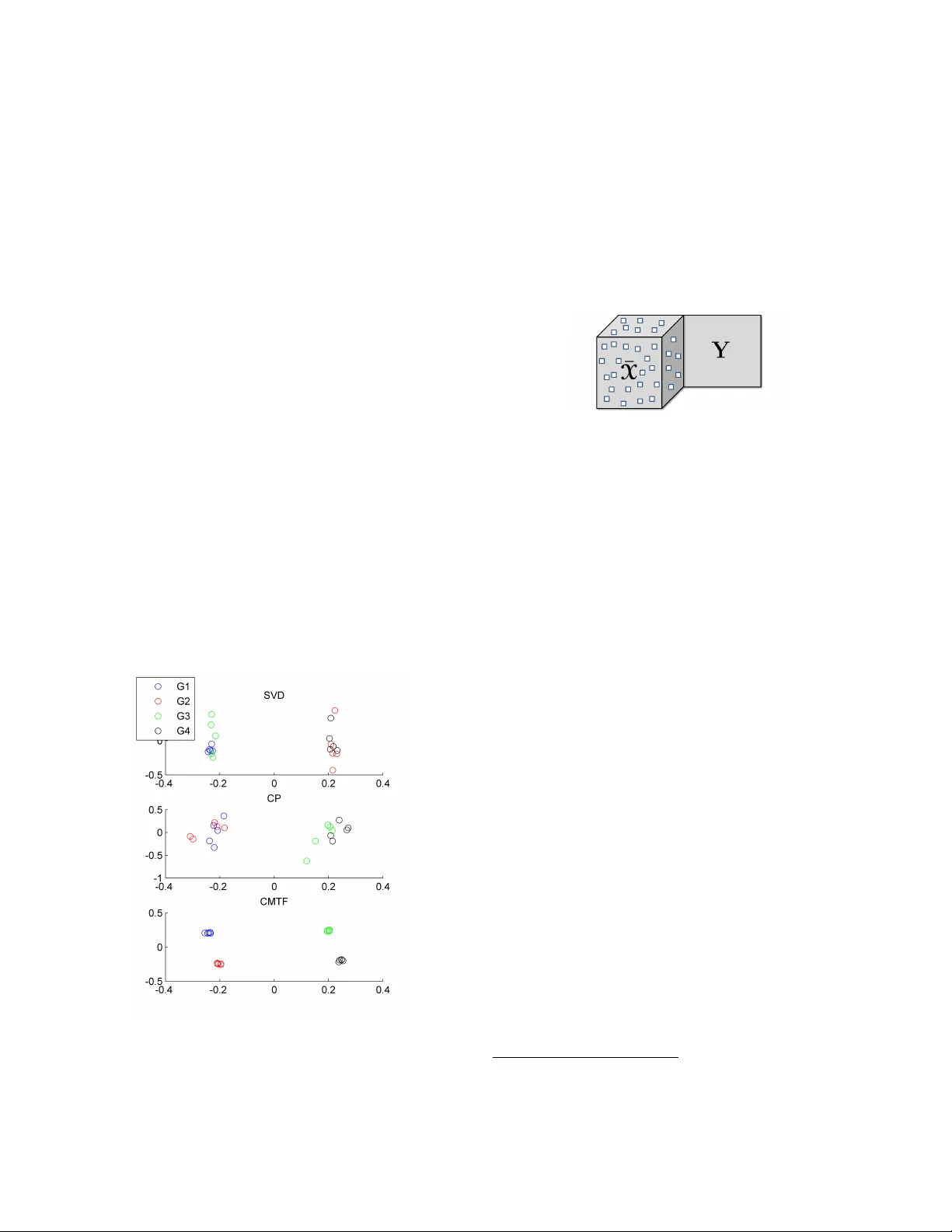
All-at-once Optimization f or Coupled Matrix and T ensor F actorizations Evrim Acar F aculty of Life Sciences, University of Copenhagen e vrim@life .ku.dk T amara G. K olda Sandia National Laboratories Livermore, CA 94551-9159 tgkolda@sandia.go v Daniel M. Dunlavy Sandia National Laboratories Albuquerque , NM 87185-1318 dmdunla@sandia.gov ABSTRA CT Join t analysis of data from multiple sources has the potential to improv e our understanding of the underlying structures in complex data sets. F or instance, in restaurant recom- mendation systems, recommendations can b e based on rat- ing histories of customers. In addition to rating histories, customers’ so cial netw orks (e.g., F aceb ook friendships) and restauran t categories information (e.g., Thai or Italian) can also be used to make b etter recommendations. The task of fusing data, how ev er, is challenging since data sets can b e incomplete and heterogeneous, i.e., data consist of b oth ma- trices, e.g., the p erson by p erson so cial netw ork matrix or the r estaur ant by c ate gory matrix, and higher-order tensors, e.g., the “ratings” tensor of the form r estaur ant by me al b y p erson . In this paper, w e are particularly interested in fusing da ta sets with the goal of capturing their underlying latent struc- tures. W e form ulate this problem as a coupled matrix and tensor factorization (CMTF) problem where heterogeneous data sets are mo deled b y fitting outer-pro duct models to higher-order tensors and matrices in a coupled manner. Un- lik e traditional approaches solving this problem using al- ternating algorithms, w e prop ose an all-at-once optimiza- tion approach called CMTF-OPT (CMTF-OPTimization), whic h is a gradien t-based optimization approac h for joint analysis of matrices and higher-order tensors. W e also ex- tend the algorithm to handle coupled incomplete data sets. Using numerical exp erimen ts, we demonstrate that the pro- posed all-at-once approac h is more accurate than the alter- nating least squares approach. K eywords data fusion, matrix factorizations, tensor factorizations, CAN- DECOMP/P ARAF AC, missing data 1. INTR ODUCTION With the abilit y to access massiv e amoun ts of data as a re- sult of recen t tec hnological a dv ances, e.g., the In ternet, com- m unication and multi-media devices, genomic technologies and new medical diagnostic technique s, w e are faced with data sets from multiple sources. F or instance, in restaurant recommendation systems, online review sites like Y elp hav e access to shopping histories of customers, friendship net- w orks of those customers, as well as categorizations of the restauran ts. Similarly , for medical diagnoses, sev eral t yp es of data are collected from a patient; for example, EEG (elec- troencephalogram) and ECG (electro cardiogram) monitor- Figure 1: Coupled Data Sets of Different Orders. Eac h ten- sor en try indicates the rating of a customer for a specific meal (i.e., breakfast, lunc h, dinner) at a particular restau- ran t. Matrices Y and Z show restaurant categories (i.e., Thai, Chinese, Italian) and social netw ork information, re- spectively . Thus, the third-order tensor X of t yp e r estaur ant b y me al b y customer can b e coupled with the r estaur ant by c ate gory matrix Y and the customer by customer matrix Z . ing data, fMRI (functional Magnetic Resonance Imaging) scans, and other data gathered from lab oratory tests. Analysis of data from multiple sources requires handling of data sets of differen t orders [7, 25, 30], i.e., matrices and/or higher-order tensors. F or instance, Banerjee et al. [7], dis- cusses the problem of analyzing heterogeneous data sets wit h a goal of sim ultaneously clustering different classes of enti- ties based on mul tiple relations, where each relation is rep- resen ted as a matrix (e.g., movies by r eview wor ds matrix sho wing movie reviews) or a higher-order tensor (e.g., movies b y viewers by actors tensor showing viewers’ ratings). Sim- ilarly , coupled analysis of matrices and tensors has been a topic of interest in the areas of communit y detection [22], collaborative filtering [36], and chemometrics [30]. As an example of data sets from m ultiple sources, without loss of generality , suppose we hav e a third-order tensor, X ∈ R I × J × K , and a matrix, Y ∈ R I × M , coupled in the first dimension (mode) of eac h. The common latent structure in these data sets can be extracted through coupled matrix and tensor factorization (CMTF), where an R -component CMTF mo del of a tensor X and a matrix Y is defined as: f ( A , B , C , V ) = k X − J A , B , C K k 2 +    Y − AV T    2 , (1) where matrices A ∈ R I × R , B ∈ R J × R and C ∈ R K × R are the factor matric es of X extracted using a CANDE- COMP/P ARAF A C (CP) mo del [10, 13, 15]. The CP model is one of the most commonly used tensor mo dels in the lit- erature (for a list of CP applications, see reviews [3, 19]). Here, w e use the notation X = J A , B , C K to denote the CP model. Similarly , matrices A and V ∈ R M × R are the factor matrices extracted from matrix Y through matrix factor- ization. The form ulation in (1) easily extends to multiple matrices and tensors, e.g., as shown in Figure 1. W e also note that we fo cus on the least squares error in this pap er, but our algorithms can b e extended to other loss functions suc h as Bregman information metric used in, e.g., [7]. W e briefly illustrate tw o motiv ating applications of coupled ma- trix and tensor factorizations. Example 1: Clustering. Joint analysis of data from mul- tiple sources may capture fine-grained clusters that would not b e captured by the individual analysis of each data set. Suppose that there is a set of customers and there are tw o sources of information ab out these customers, X ∈ R I × J × K and Y ∈ R I × M , one storing information ab out which items customers ha ve b ought ov er a p eriod of time, and the other sho wing where customers live. Within this set of customers, there are 4 groups: { G 1 , G 2 , G 3 , G 4 } and each group consists of people who liv e in the same neigh b orho od and ha ve an in- terest in similar items. Imagine that the matrix Y can only discriminate betw een ( G 1 ∪ G 3 ) a nd ( G 2 ∪ G 4 ). A rank-2 ma- trix SVD factorization of Y w ould yield factors that could be used to cluster the customers as in the top plot shown in Figure 2 (SVD), failing to fully separate the four groups. Con versely , imagine that the tensor X only has enough in- formation to discriminate b et ween ( G 1 ∪ G 2 ) and ( G 3 ∪ G 4 ). In this case, a rank-2 CP factorization of the tensor would still only separate the data into tw o groups, alb eit tw o dif- feren t groups, as illustrated in the middle plot in Figure 2 (CP). If, ho w ever, w e join tly factor the matrix and tensor sim ultaneously using CMTF, the four group s are completely separated, as sho wn in the bottom plot of Figure 2 (CMTF). Details of the data generation for this example are provided in the appendix.  Figure 2: Clustering based on matrix SVD factorization of Y vs. CP tenso r factorization of X vs. c oupled matrix-tensor factorization of X and Y . The subplots presen t the scatter plots showing the first factor plotted against the second fac- tor in the first mode. Example 2: Missing Data Recov ery . CMTF can b e used for missing data recov ery when data from different sources hav e the same underlying lo w-rank structure (at least in one mode) but some of the data sets hav e miss- ing entries (Figure 3). If a matrix or a higher-order tensor has a lo w-rank structure, it is possible to reco ver the missing en tries using a limited num b er of data entries [1, 9]. Ho w- ev er, if there is a large amoun t of missing data, then the analysis of a single data set is no longer enough for accu- rate data reco very . Here, we pro vide an example illustrating that missing entries can still b e recov ered accurately using CMTF even when the analysis of a single data set fails to do so. Figure 3: Incomplete tensor ¯ X and matrix Y coupled in the first mo de. Suppose w e hav e a tensor X and a matrix Y computed as X = J A , B , C K and Y = AV T , where matrices A ∈ R I × R , B ∈ R J × R , C ∈ R K × R and V ∈ R M × R are generated using random entries dra wn from the standard normal distribu- tion. ¯ X ∈ R I × J × K is constructed by randomly setting M % of the en tries of X to b e missing, i.e., ¯ X = W ∗ X , where the binary tensor W is the same size as tensor X and w ij k = 0 if we wan t to set x ij k to missing. In order to reco ver the missing entries, one approach is to fit an R -component CP model to ¯ X and use the extracted factors to recov er missing en tries. An alternative approach is to fit an R -component CMTF mo del to ¯ X and Y b y extracting a common factor matrix in the first mode and then mak e use of CMTF factors to recov er the missing entries. Figure 4 illustrates how the recov ery error behav es for differen t amoun ts of missing data. W e observ e that CP is accurate in terms of reco verin g missing entries if less than 80% of the entries are missing. Ho wev er, there is a sharp in error as we further increase the amount of missing entries. On the other hand, CMTF can compute factors with low reco very error for higher amounts of missing data; only for problems with more that 90% missing data does the recov ery error increase 1 .  In order to solve coupled matrix and tensor factorization, v arious algorithms hav e b een proposed in the literature us- ing a v ariety of loss functions [7, 22]. These algorithms all propose an alternating scheme, where the basis for each en- tit y t yp e is determined one at a time. In this pap er, we focus solely on the L 2 loss function, which is often solved using alternating least squares (ALS). Esp ecially when fit- ting tensor models, ALS is the most commonly used algo- rithm due to its sp eed and ease of implementation. On the other hand, ALS suffers from several problems: (i) It ma y fail to find the underlying components accurately if the n um- ber of comp onen ts is not correctly estimated [2, 32]; (ii) In 1 Note that the amount of missing data where the reco very error mak es a sharp increase may change dep ending on the v alues of I , J, K, V and R . F or example, with small data sizes and large R , dealing with missing data is challeng ing[1]. Figure 4: Missing data recov ery using CP factorization of ¯ X vs. CMTF of ¯ X and Y . T ensor Completion Score is the recov ery error measure used here and is defined as k (1 − W ) ∗ ( X − ˆ X ) k k (1 − W ) ∗ X k , where ˆ X corresp onds to the data recon- structed using the extracted factor matrices, i.e., ˆ A , ˆ B , and ˆ C , as ˆ X = J ˆ A , ˆ B , ˆ C K . the presence of missing data, ALS-based imputation tech- niques ma y suffer from po or con vergence [8] and do not scale to large-scale data sets [1]. Therefore, unlike the previous w ork using alternating least squares algorithms, we prop ose an all-at- once optimization approach solving for all v ariables sim ultaneously . Our con tributions in this pap er are • Developing an algorithm called CMTF-OPT (CMTF- OPTimization) based on first-order optimization to solv e coupled matrix and tensor factorization problem for a giv en num b er of comp onents ( R ). 2 • Extending CMTF-OPT algorithm to handle incom- plete data sets, i.e., data with missing or unknown en tries. • Demonstrating that CMTF-OPT is more accurate than an alternating least squares approach using nu merical experiments. This paper is organized as follo ws. In § 2, w e in troduce the notation for tensors and tensor operations. After discussing the related w ork on coupled data analysis in § 3, w e in troduce our CMTF-OPT algorithm and its extension to data with missing en tries in § 4. Section 5 describ es n umerical exp er- imen ts and demonstrates ho w CMTF-OPT compares with CMTF-ALS in terms of capturing the underlying factors in coupled data sets. Finally , w e conclude with future research directions in § 6. 2. NO T A TION AND B A CKGR OUND T ensors of order N ≥ 3 are denoted b y Euler script letters ( X , Y , Z ), matrices are denoted b y boldface capital letters ( A , B , C ), v ectors are denoted by b oldface low ercase letters ( a , b , c ), and scalars are denoted by low ercase letters ( a , b , c ). Col umns of a matrix are denoted by b oldface lo wer letters with a subscript, e.g., a r is the rth column of matrix A . Entries of a matrix or a tensor are denoted by low ercase letters with subscripts, i.e., the ( i 1 , i 2 , . . . , i N ) entry of an 2 Determining the num b er of comp onen ts R in CMTF re- mains as a challenge just lik e computing the tensor rank, whic h is NP-hard [14]. N -w ay tensor X is denoted by x i 1 i 2 ··· i N . Giv en a matrix A of size I × J , vec ( A ) stac ks the columns of the matrix and forms a vector of length I J : vec ( A ) =     a 1 . . . a J     ∈ R I J . Giv en t wo matrices A ∈ R I × K and B ∈ R J × K , their Khatri-Rao product is denoted by A  B and defined as column wise Kroneck er pro duct. Th e result is a matrix of size ( I J ) × K and defined by A  B =  a 1 ⊗ b 1 a 2 ⊗ b 2 · · · a K ⊗ b K  , where ⊗ denotes Kroneck er pro duct. F or more details on properties of Kroneck er and Khatri-Rao pro ducts, see [19]. An N -wa y tensor can b e rearranged as a matrix; this is called matricization . The mode- n matricization of a ten- sor X ∈ R I 1 × I 2 ×···× I N is denoted by X ( n ) and arranges the mode- n one-dimensional “fib ers” to b e the columns of the resulting matrix. Giv en tw o tensors X and Y of equal size I 1 × I 2 × · · · × I N , their Hadamard (element wise) pro duct is denoted by X ∗ Y and defined as ( X ∗ Y ) i 1 i 2 ··· i N = x i 1 i 2 ··· i N y i 1 i 2 ··· i N for all i n ∈ { 1 , . . . , I n } and n ∈ { 1 , . . . , N } . Their inner product, denoted by h X , Y i , is the sum of the products of their entries, i.e., h X , Y i = I 1 X i 1 =1 I 2 X i 2 =1 · · · I N X i N =1 x i 1 i 2 ··· i N y i 1 i 2 ··· i N . F or a tensor X of size I 1 × I 2 × · · · × I N , its norm is k X k = p h X , X i . F or matrices and v ectors, k · k refers to the anal- ogous F robenius and tw o-norm, resp ectiv ely . Giv en a sequence of matrices A ( n ) of size I n × R for n = 1 , . . . , N , the notation J A (1) , A (2) , . . . , A ( N ) K defines an I 1 × I 2 × · · · × I N tensor whose elemen ts are given by  J A (1) , A (2) , . . . , A ( N ) K  i 1 i 2 ··· i N = R X r =1 N Y n =1 a ( n ) i n r , for i n ∈ { 1 , . . . , I n } , n ∈ { 1 , . . . , N } . F or just tw o matrices, this reduces to J A , B K = AB T . 3. RELA TED WORK IN D A T A FUSION Data fusion, also called collective data analysis, multi- block, m ulti-view or multi-set data analysis, has been a topic of in terest in different fields for decades. First, we briefly dis- cuss data fusion techniques for multipl e data sets eac h rep- resen ted as a matrix and then fo cus on techniques proposed for coupled analysis of heterogenous data sets. 3.1 Collective Factorization of Matrices The analysis of data from multiple sources attracted con- siderable atten tion in the data mining communit y during the Netflix Prize comp etition [20], where the goal w as to mak e accurate predictions ab out mo vie ratings. In order to achiev e better rating predictions, additional data sources complemen ting user ratings suc h as tagging information ha ve been exploited; e.g., users tag movies [33] as well as features of movies such as mo vie t yp es or mo vie pla yers . Singh and Gordon [28] proposed Collective Matrix F actorization (CMF) to tak e adv an tage of correlations b et ween different data sets and sim ultaneously factorize coupled matrices. Gi- v en tw o matrices X and Y of size I × M and I × L , resp ec- tiv ely , CMF can b e formulated as f ( U , V , W ) =    X − UV T    2 +    Y − UW T    2 , (2) where U , V and W are factor matrices of size I × R , M × R and L × R , respectively and R is the num b er of factors. This formula tion is a sp ecial case of the general approach in tro duced in [28], which extends to different loss functions. Earlier, Long et al. [24, 23] had also studied collective matrix factorization using a differen t matrix factorization scheme than X = UV T . The prop osed approac hes in those studies are based on alternating algorithms solving the collectiv e factorization problem for one factor matrix at a time. Analysis of mu ltiple matrices dates bac k to one of the earliest mo dels aiming to capture the common v ariation in t wo data sets, i.e., Canonical Correlation Analysis (CCA) [16]. Later, other studies follow ed CCA by extending it to more than t wo data sets [18], fo cusing on simultaneous fac- torization of Gramian matrices [21] and working on PCA of m ultiple matrices [17, 34]. Moreo ver, several approaches for sim ultaneous factor analysis ha ve b een dev elop ed for sp e- cific applications as well; e.g., p opulation differentiation in biology [31], blind source separation [37], multimicrop hone speech filtering [11], and microarray data analysis [4, 5, 6]. T ensor factorizations [3, 19, 29] can also b e considered as one wa y of analyzing multiple matrices. F or instance, when a tensor mo del is fit to a third-order tensor, m ultiple coupled matrices are analyzed simultaneously . Nev ertheless, neither CMF nor tensor factorizations can handle coupled analysis of heterogeneous data, which we address next. 3.2 Collective Factorization of Mixed Data As describ ed in § 1, heterogeneous data consists of data sets of different orders, i.e., b oth matrices and higher-order tensors. The formulation in (2) can b e extended to het- erogeneous data sets: Given a tensor X and a matrix Y of sizes I × J × K and I × M , resp ectively , we can formu- late their factorization coupled in the first mode as shown in (1). Note that (1) can b e considered as a sp ecial case of the approach introduced b y Smilde et al. [30] for multi-w a y m ulti-blo c k data analysis, where different tensor models can be fit to higher-order data sets and the factor matrices cor- responding to the coupled mo des do not necessarily match. The same formulation as in (1) has recent ly b een studied in psyc hometrics as Linked-Mode P ARAF A C-PCA [35]. As a more general framework, not restricted to squared Euclidean distance, Banerjee et al. [7] introduced a multi -wa y cluster- ing approach for relational and m ulti-relational data where coupled analysis of m ultiple data sets including higher-order data sets w ere studied using minim um Bregman informa- tion. The pap er [22] also discussed coupled analysis of mul- tiple tensors and matrices using nonnegativ e factorization b y formulat ing the problem using KL-divergence. All these studies propose algorithms that are based o n alternating ap- proac hes. In this pap er we fo cus on the squared Euclidean distance as the loss function as in (1). Rewriting X = J A , B , C K as X (1) = A ( C  B ) T , X (2) = B ( C  A ) T , etc., for the differen t while not “conv erged” do rescale all factors to unit F robenious norm solv e for A (for fixed B , C , V ) min A    X (1) Y  − A  ( C  B ) T V T    2 solv e for B (for fixed A , C , V ) min B   X (2) − B ( C  A ) T   2 solv e for C (for fixed A , B , V ) min C   X (3) − C ( B  A ) T   2 solv e for V (for fixed A , B , C ) min V   Y − AV T   2 end while Figure 5: CMTF-ALS: Alternating Least Squares Algorithm for coupled matrix and tensor factorization of a third-order tensor X and matrix Y coupled in the first mo de. modes of X , we summarize the steps of an alternating least squares algorithm for solving (1) in Figure 5. The main loop in the algorithm is often terminated as a function of the relative change in function v alue (e.g., as defined b elo w in (5)), a function of the relative cha nge in factor matrices, and/or after a prescrib ed num b er of iterations. ALS-based algorithms are simple to implement and com- putationally efficient; ho wev er, ALS has shown to b e error- prone when fitting a CP mo del in the case of ov erfactoring, i.e., the num b er of extracted components is more than the true n umber of underlying co mp onen ts [2, 32]. F urthermore, in the presence of missing data, ALS-based techniques ma y ha ve po or con vergence [8] and do not scale to very large data sets [1]. On the other hand, all-at-once optimization, in other words, solving for all CP factor matrices simultane- ously has shown to b e more robust to o verfactoring [2, 32] and easily extends to handle data with missing entries even for very large data sets [1]. Therefore, in order to deal with these issues, w e develop an algorithm called CMTF-OPT, whic h form ulates coupled ana lysis of heterogeneous data sets just like [30, 35] but solves for all factor matrices simultane- ously using a gradient-based optimization approac h. 4. CMTF-OPT ALGORITHM In this section, we consider join t analysis of a matrix and an N th-order tensor with one mo de in common, where the tensor is factorized using an R -component CP model and the matrix is factorized by extracting R factors using ma- trix factorization. Let X ∈ R I 1 × I 2 ×···× I N and Y ∈ R I 1 × M ha ve the nth mode in common, where n ∈ { 1 , . . . , N } . The ob jective function for coupled an alysis of these tw o data se ts is defined b y f ( A (1) , A (2) , . . . , A ( N ) , V ) = 1 2    X − J A (1) , . . . , A ( N ) K    2 + 1 2    Y − A ( n ) V T    2 (3) Our goal is to find the matrices A ( i ) ∈ R I i × R for i = 1 , 2 , ...N and matrix V ∈ R M × R that minimize the ob jective in (3). In order to solv e this optimization problem, we can compute the gradient and then use any first-order optimiza- tion algorithm [27]. Next, we discuss the computation of the gradien t for (3). W e can rewrite (3) as tw o components, f 1 and f 2 : f = 1 2    X − J A (1) , . . . , A ( N ) K    2 | {z } f 1 ( A (1) , A (2) ,..., A ( N ) ) + 1 2    Y − A ( n ) V T    2 | {z } f 2 ( A ( n ) , V ) The partial deriv ative of f 1 with resp ect to A ( i ) has b een deriv ed in [2] so we just present the results here. Let Z = J A (1) , . . . , A ( N ) K , then ∂ f 1 ∂ A ( i ) = ( Z ( i ) − X ( i ) ) A ( − i ) where A ( − i ) = A ( N )  · · ·  A ( i +1)  A ( i − 1)  · · ·  A (1) , for i = 1 , . . . , N . The partial deriv atives of the second comp onen t, f 2 , with respect to A ( i ) and V can be computed as ∂ f 2 ∂ A ( i ) = ( − Y V + A ( − i ) V T V , for i = n, 0 for i 6 = n, ∂ f 2 ∂ V = − Y T A ( i ) + VA ( i ) T A ( i ) . Com bining the ab ov e results, we can compute the partial deriv ative of f with resp ect to factor matrix A ( i ) , for i = 1 , 2 , ..., N , and V as: ∂ f ∂ A ( i ) = ∂ f 1 ∂ A ( i ) + ∂ f 2 ∂ A ( i ) ∂ f ∂ V = ∂ f 2 ∂ V Finally , the gradien t of f , whic h is a vector of size P = R ( P N n =1 I n + M ), can b e formed by vectorizing the partial deriv atives with resp ect to each factor matrix and concate- nating them all, i.e., ∇ f =         vec  ∂ f ∂ A (1)  . . . vec  ∂ f ∂ A ( N )  vec  ∂ f ∂ V          4.1 CMTF-OPT for Incomplete Data In the presence of missing data, it is still p ossible to do coupled analysis by ignoring the missing entries and fitting the tensor and/or the matrix model to the known data en- tries. Here we study the case where tensor X has missing en tries as in Figure 3. Let W ∈ R I 1 × I 2 ×···× I N indicate the missing entries of X suc h that w i 1 i 2 ··· i N = ( 1 if x i 1 i 2 ··· i N is known , 0 if x i 1 i 2 ··· i N is missing , for all i n ∈ { 1 , . . . , I n } and n ∈ { 1 , . . . , N } . W e can then modify the ob jective function (3) as f W ( A (1) , A (2) , . . . , A ( N ) , V ) = 1 2    W ∗  X − J A (1) , . . . , A ( N ) K     2 | {z } f W 1 ( A (1) , A (2) ,..., A ( N ) ) + 1 2    Y − A ( n ) V T    2 The first term, f W 1 , corresp onds to the weigh ted least squares problem for fitting a CP mo del while the second term stays the same as in (3). The partial deriv ativ e of f W 1 with resp ect to A ( i ) can b e computed as in [1] as ∂ f W 1 ∂ A ( i ) =  W ( i ) ∗ Z ( i ) − W ( i ) ∗ X ( i )  A ( − i ) , for i = 1 , . . . , N . Since the partial deriv atives of the second term do not c hange, we can write the partials of f with respect to A ( i ) for i = 1 , 2 , ..., N , and V as: ∂ f W ∂ A ( i ) = ( ∂ f W 1 ∂ A ( i ) for i ∈ { 1 , . . . , N } / { n } , ∂ f W 1 ∂ A ( i ) + ∂ f 2 ∂ A ( i ) for i = n. ∂ f W ∂ V = ∂ f 2 ∂ V The gradient of f W , ∇ f W , is also a vecto r of size P = R ( P N n =1 I n + M ) and can b e formed in the same wa y as ∇ f . Once we hav e the function, f (or f W ), and gradient, ∇ f (or ∇ f W ), v alues, we can use any gradien t-based optimiza- tion algorithm to compute the factor matrices. F or the re- sults presented in this pap er, w e use the Nonlinear Con- jugate Gradient (NCG) with Hestenes-Stei fel updates [27] and the Mor´ e-Th uente line search [26] as implemen ted in the Poblano T oolb o x [12]. 5. EXPERIMENTS W e compare the p erformance of the prop osed CMTF- OPT algorithm with the ALS-based approach (i.e., CMTF- ALS as shown in Figure 5) in terms of accuracy using ran- domly generated matrices and tensors. Our goal is to see whether the algorithms can capture the underlying factors in the data (i) when ¯ R = R factors are extracted, and (ii) in the case of o verfac toring, e.g., when ¯ R = R + 1 factors are extracted, where ¯ R and R denote the extracted and true n umber of factors. 5.1 Data Generation In our experiments, three differen t scenarios are used (see T able 1). In the first case, we hav e a tensor X and a matrix Y coupled in the first mo de. In the second case, w e hav e t wo third-order tensors X and Y coupled in one dimension. The third case has a third-order tensor X and tw o matrices Y and Z such that the tensor shares one mo de with each one of the matrices. T o construct the tensors and matrices in eac h scenario, random factor matrices with entries follo wing standard nor- mal distribution are generated and a tensor (or a matrix) is formed based on a CP (or a matrix) mo del. F or ex- ample, for the first scenario, w e generate random factor matrices A ∈ R I × R , B ∈ R J × R and C ∈ R K × R , and form a third-order tensor X ∈ R I × J × K based on a CP model. Gaussian noise is later added to the tensor, i.e., X = J A , B , C K + η N k J A , B , C K k k N k , where N ∈ R I × J × K cor- responds to the random noise tensor and η is used to ad- just the noise lev el. Similarly , we generate a factor matrix V ∈ R I × R and form matrix Y = AV T + η N k AV T k k N k . The matrix N ∈ R I × R is a matrix with entries dra wn from the standard normal distribution and is used to introduce dif- fering amoun ts of noise in the data. In our experiments, w e use three different noise levels, i.e., η = 0 . 1 , 0 . 25 and 0 . 35, and the true num ber of factors is R = 3. 5.2 Perf ormance Metric W e fit an ¯ R -comp onen t CMTF mo del using CMTF-OPT and CMTF-ALS algorithms, where ¯ R = R and ¯ R = R + 1, and compare the algorithms in terms of accuracy; in other words, how well the factors extracted by the algo- rithms match with the original factors used to generate the data. F or instance, for the first scenario describ ed abov e, let A , B , C and V b e the original factor matrices and ˆ A , ˆ B , ˆ C and ˆ V b e the extracted factor matrices. W e quantify ho w w ell the extracted factors matc h with the original ones using the factor matc h score (FMS) defined as follows: FMS = min r (1 − | ξ r − ˆ ξ r | max( ξ r , ˆ ξ r ) ) | a T r ˆ a r b T r ˆ b r c T r ˆ c r v T r ˆ v r | . (4) Here, the columns of factor matrices are normalized to unit norm and ξ r denotes the w eight for each factor r , for r = 1 , 2 , ...R . The weigh t for each factor is computed as follows: W e can rewrite X = J A , B , C K as X = P R r =1 λ r a r ◦ b r ◦ c r , where ◦ denotes n -mo de vector outer pro duct; the columns of the factor matrices are normalized to unit norm and λ r is the pro duct of the v ector norms in each mode. Similarly , we can rewrite Y = AV T as Y = P R r =1 α r a r ◦ v r b y normaliz- ing the matrix columns and using α r to denote the pro duct of vector norms. W e define the norm of eac h CMTF com- ponent, i.e., ξ r , as ξ r = λ r + α r . In (4), ξ r and ˆ ξ r indicate the weigh ts corresponding to the original and extracted r th CMTF component, resp ectively . If the extracted and origi- nal factors p erfectly match, FMS v alue will be 1. It is also considered a success if FMS is abov e a certain thresho ld, i.e., (0 . 99) N , where N is the num b er of factor matrices. 5.3 Stopping Conditions As a stopping condition, b oth algorithms use the relative c hange in function v alue and stop when | f current − f previous | f previous ≤ 10 − 8 , (5) where f is as giv en in (3). Additionally , for CMTF-ALS, the maxim um num b er of iterations is set to 10 4 . F or CMTF- OPT, the maximum n umber of function v alues (which cor- responds the num b er of iterations in an ALS algorithm) is set to 10 4 and the maximu m n umber of iterations is set to 10 3 . CMTF-OPT also uses the tw o-norm of the gradien t divided b y the num ber of entries in the gradien t and the tolerance for that is set to 10 − 8 . In the exp eriments, the al- gorithms ha ve generally stopp ed due to the relative change in function v alue criterion. Ho wev er, w e also rarely observ e that b oth CMTF-OPT and CMTF-ALS hav e stopp ed since the algorithms hav e reac hed the maxim um num b er of itera- tions, i.e., appro ximately 2% of all runs for CMTF-OPT and 0 . 3% of all runs for CMTF-ALS. F urthermore, for around 2% of all runs, CMTF-OPT has stopp ed b y satisfying the condition on the gradient. 5.4 Results W e demonstrate the p erformance of the algorithms in terms of accuracy in T able 1 and T able 2. T able 1 presents the results for the exp eriments where factor matrices are generated with columns normalized to unit norm. F or in- stance, for the example discussed ab o v e, this corresp onds to generating tensor X and matrix Y using λ r = α r = 1, for r = 1 , 2 , ..R . In T able 1, for all different scenarios, we ob- serv e that when the correct n umber of underlying factors are extracted, i.e., ¯ R = R , the success ratios of b oth algorithms are compatible. Since w e repeat our experiments with 30 dif- feren t sets of factor matrices for eac h set of parameters, we report the av erage factor match score for 30 runs. The av er- age scores for b oth algorithms are quite close and p-v alues computed for paired-sample t -tests indicate that differences in the scores are not statistically significan t. On the other hand, for all scenarios, when we lo ok at the cases where the data is o verfactored, i.e., ¯ R = R + 1, CMTF-OPT signif- ican tly outp erforms CMTF-ALS. While CMTF-OPT algo- rithm is quite accu rate in terms of reco vering the underlying factors in the case of ov erfactoring, the accuracy of CMTF- ALS is quite low. W e also observ e that the increase in the noise level barely affects the accuracies of the algorithms. In T able 2, we presen t the results for a harder set of ex- periments, where the norm of eac h tensor and matrix com- ponent, i.e., λ r , α r for r = 1 , 2 , ..R , is a randomly assigned in teger greater than or equal to 1. 3 Similar to the previous case, we observ e that CMTF-OPT is more robust to ov er- factoring compared to CMTF-ALS. Ho wev er, the accuracies reported in this table are low er compared to T able 1. In particular, as the noise level increases, it b ecomes harder to find the underlying comp onen ts and accuracies drop even if the tru e n um b er of unde rlying factors are extracted from the data. F or instance, for the first scena rio, when the noise level is 0.35, the accuracy of CMTF-OPT is 60% for the case we extract the correct num b er of comp onents. This is in part due to not being able to find ξ r , for r = 1 , 2 , ..R , accurately . If we sligh tly c hange the FMS such that w e only require min r | a T r ˆ a r b T r ˆ b r c T r ˆ c r v T r ˆ v r | to b e greater than the threshold, then the av erage accuracy go es up to around 73%. The rest of the failing runs is due to the fact that extracted factors are distorted compared to the original factors used to gen- erate the data. Note that factor match scores are still high whic h indicates that the factors are only slightly distorted. 6. CONCLUSIONS W e hav e seen a shift in data mining in recent years: from models fo cusing on matrices to those studying higher-order tensors and now w e are in need of mo dels to explore and ex- tract the underlying structures in data from multiple sources. One approach is to formulate this problem as a coupled ma- trix and tensor factorization problem. In this paper, we address the problem of solving coupled matrix and tensor factorizations when we ha ve squared Euclidean distance as the loss function and introduce a first-order optimization al- gorithm called CMTF-OPT, whic h solv es for all factor ma- trices in all data sets sim ultaneously . W e ha v e also extended our algorithm to data with missing entries by introducing CMTF-W OPT for the case where w e ha ve an incomplete higher-order tensor coupled with matrices. The algorithm can easily be extended to multi ple incomplete data sets. T o the b est of our kno wledge, the algorithms proposed so far for fitting a coupled matrix and tensor factorization model hav e all b een alternating algorithms. W e ha ve com- pared our CMTF-OPT algorithm with a traditional alter- 3 Eac h norm is c hosen as the absolute v alue of a n umber ran- domly chosen from N (0 , 25) rounded to the nearest in teger plus 1. T able 1: Comparison of CMTF-OPT and CMTF-ALS for the cases where λ r = α r = ... = 1, for r = 1 , 2 , ...R . Noise ¯ R ALG. Success Mean p-v al Success Mean p-v al Success Mean p-v al (%) FMS (%) FMS (%) FMS η = 0.10 R OPT 100.0 1.00 9.3e-1 96.7 0.97 1.0 100.0 1.00 3.3e-1 ALS 100.0 1.00 96.7 0.97 96.7 0.9 6 R + 1 OPT 96.7 0.9 7 3.3e-13 100.0 1.00 1.6e-8 96.7 0.97 3.8e-24 ALS 3.3 0.29 6.7 0.71 0.0 0.06 η = 0.25 R OPT 100.0 0.99 4.5e-1 100.0 1.00 0.2e-1 96.7 0.96 3.3e-1 ALS 100.0 0.99 100.0 1.00 100.0 0.99 R + 1 OPT 100.0 0.99 2.6e-11 100.0 1.00 1.8e-7 100.0 0.99 7.0e-16 ALS 6.7 0.34 16.7 0.70 10.0 0.14 η = 0.35 R OPT 100.0 0.99 5.8e-1 100.0 1.00 3.3e-1 100.0 0.99 3.6e-1 ALS 100.0 0.99 96.7 0.97 100.0 0.99 R + 1 OPT 90.0 0.92 1.8e-5 100.0 1.00 1.0e-7 86.7 0.88 2.9e-5 ALS 33.3 0.55 13.3 0.71 36.7 0.39 T able 2: Comparison of CMTF-OPT and CMTF-ALS for the cases where λ r , α r , ... ≥ 1 for r = 1 , 2 , ...R . Noise ¯ R ALG. Success) Mean p-v al Success Mean p-v al Success Mean p-v al (%) FMS (%) FMS (%) FMS η = 0.10 R OPT 96.7 0.96 3.3e-1 100.0 1.00 9.1e-1 96.7 0.96 3.3e-1 ALS 100.0 0.99 100.0 1.00 90.0 0.90 R + 1 OPT 90.0 0.96 1.5e-13 100.0 1.00 6.8e-9 83.3 0.89 1.6e-11 ALS 3.3 0.24 13.3 0.52 10.0 0.13 η = 0.25 R OPT 76.7 0.97 3.3e-1 96.7 0.97 1.0 83.3 0.97 0.4e-1 ALS 73.3 0.94 96.7 0.97 70.0 0.84 R + 1 OPT 86.7 0.97 6.4e-9 100.0 1.00 7.8e-5 76.7 0.90 1.4e-8 ALS 13.3 0.40 46.7 0.72 10.0 0.23 η = 0.35 R OPT 60.0 0.95 3.6e-1 100.0 1.00 3.3e-1 53.3 0.92 7.4e-1 ALS 56.7 0.95 96.7 0.97 53.3 0.92 R + 1 OPT 46.7 0.87 1.7e-9 100.0 1.00 4.0e-6 50.0 0.83 4.9e-7 ALS 6.7 0.35 40.0 0.62 10.0 0.30 nating least squares approach and the numerical results sho w that all-at-once optimi zation is more robust to ov erfactoring as it has also been the case for fitting tensor mo dels [2, 32]. Note that our current formulation of coupled matrix and tensor factorization has one drawbac k, whic h is encountered when we hav e a data set whose factor matrices are shared b y all other data sets. F or instance, we may hav e a tensor X , where X = J A , B , C K = P R r =1 λ r a r ◦ b r ◦ c r and tw o matrices Y = AV T = P R r =1 α r a r ◦ v r and Z = BV T = P R r =1 β r b r ◦ v r . If w e form ulate a coupled factorization for these data sets as f ( A , B , C , V ) = k X − J A , B , C K k 2 +   Y − AV T   2 +   Z − BV T   2 , we do not take into accoun t the cases for λ r 6 = α r 6 = β r . F or such scenarios, scaling am- biguities should b e taken into consideration by introducing a set of parameters for the scalars in the formulation. Another issue we hav e not addressed in this pap er is how to weigh different parts of the ob jective function modeling differen t data sets as discussed in [35]. This is an area of future researc h where a Bay esian framew ork for co upled ma- trix and tensor factorizations may be a promising approach. As another area of future researc h, w e plan to extend our ap- proac h to different loss functions in order to b e able to deal with different types of noise and incorp orate nonnegativit y constrain ts on the factors as nonnegativity often improv es the interpretabilit y of the mo del. 7. A CKNO WLEDGMENTS This work was supp orted in part by the Lab oratory Di- rected Research and Developmen t program at Sandia Na- tional Lab oratories. Sandia National Lab oratories is a m ulti- program lab oratory managed and operated b y Sandia Cor- poration, a wholly owned subsidiary of Lockheed Martin Corporation, for the U.S. Department of Energy’s National Nuclear Securit y Administration under contract DE-AC04- 94AL85000. 8. REFERENCES [1] E. Acar, D. Dunla vy , T. Kolda, and M. Morup. Scalable tensor factorizations for incomplete data. Chemometrics and Intel ligent Lab or atory Systems , 106:41–56, 2011. [2] E. Acar, D. M. Dunlavy , and T. G. Kolda. A scalable optimization approach for fitting canonical tensor decompositions. J. Chemometrics , 25:67–86, 2011. [3] E. Acar and B. Y ener. Unsup ervised multiw a y data analysis: A literature survey . IEEE T r ans. Know le dge and Data Engine ering , 21(1):6–20, 2009. [4] O. Alter, P . O. Brown, and D. Botstein. Generalized singular v alue decomp osition for comparative analysis of genome-scale expression data sets of tw o different organisms. PNAS , 100(6):3351–3356, 2003. [5] L. Badea. Combining gene expression and transcription factor regulation data using sim ultaneous nonnegative matrix factorization. In Pr o c. BIOCOMP-2007 , pages 127–131, 2007. [6] L. Badea. Extracting gene expression profiles common to colon and pancreatic adeno carcinoma using sim ultaneous nonnegative matrix factorization. In Pacific Symp osium on Bio computi ng , pages 267–278, 2008. [7] A. Banerjee, S. Basu, and S. Merugu. Multi-wa y clustering on relation graphs. In SDM’07 , pages 145–156, 2007. [8] A. M. Buchanan and A. W. Fitzgibb on. Damp ed Newton algorithms for matrix factorization with missing data. In CVPR’05 , pages 316–322, 2005. [9] E. J. Candes and T. T ao. The p ow er of conv ex relaxation: Near-optimal matrix completion. IEEE T r ans. Information The ory , 56:2053–2080, 2009. [10] J. D. Carroll and J. J. Chang. Analysis of individual differences in m ultidimensional scaling via an N-wa y generalization of “Eck art-Y oung” decomp osition. Psychometrika , 35:283–319, 1970. [11] S. Do clo and M. Mo onen. Gsvd-based optimal filtering for single and multimicrophone sp eech enhancement. IEEE T r ansactions on Signal Pr o c essing , 50(9):2230–2244, 2002. [12] D. M. Dunlavy , T. G. Kolda, and E. Acar. P oblano v1.0: A Matlab to olb o x for gradien t-based optimization. T ec hnical Rep ort SAND2010-1422, Sandia National Lab oratories, Mar. 2010. [13] R. A. Harshman. F oundations of the P ARAF AC procedure: Models and conditions for an “explanatory” m ulti-modal factor analysis. UCLA Working Pap ers in Phonetics , 16:1–84, 1970. [14] J. H ˚ astad. T ensor rank is NP-complete. J. Algo rithms , 11(4):644–654, 1990. [15] F. L. Hitchcock. The expression of a tensor or a polyadic as a sum of pro ducts. J. Mathematics and Physics , 6(1):164–189, 1927. [16] H. Hotelling. Relations b etw een tw o sets of v ariates. Biometrika , 28:321–377, 1936. [17] H. Kargupta, W. Huang, K. Siv akumar, B.-H. Park, and S. W ang. Collectiv e principal component analysis from distributed, heterogeneous data. In PKDD’00 , pages 452–457, 2000. [18] J. R. Kettenring. Canonic al Analysis of Sever al Sets of V ariables . PhD thesis, Universi ty of North Carolina at Chapel Hill, 1969. [19] T. G. Kolda and B. W. Bader. T ensor decompositions and applications. SIAM R eview , 51(3):455–500, 2009. [20] Y. Koren, R. Bell, and C. V olinsky . Matrix factorization techniques for recommender systems. IEEE Computer , 42(8):30–37, 2009. [21] J. Levin. Simultaneous factor analysis of several gramian matrices. Psychometrika , 31:413–419, 1966. [22] Y.-R. Lin, J. Sun, P . Castro, R. Konuru, H. Sundaram, and A. Kelliher. Metafac: comm unity disco very via relational hypergraph factorization. In KDD’09 , pages 527–536, 2009. [23] B. Long, X. W u, Z. M. Zhang, and P . S. Y u. Unsupervised learning on k-partite graphs. In KDD’06 , pages 317–326, 2006. [24] B. Long, Z. M. Zhang, X. W u, and P . S. Y u. Sp ectral clustering for m ulti-type relational data. In ICML’06 , pages 585–592, 2006. [25] I. V. Mechelen and A. K. Smilde. A generic link ed-mo de decomp osition model for data fusion. Chemometrics and Intel ligent Lab or atory Systems , 104(1):83–94, 2010. [26] J. J. Mor´ e and D. J. Thuen te. Line search algorithms with guaranteed sufficien t decrease. ACM T r ans. Mathematic al Softwar e , 20(3):286–307, 1994. [27] J. No cedal and S. J. W right. Numeric al Optimization . Springer, 2006. [28] A. P . Singh and G. J. Gordon. Relational learning via collectiv e matrix factorization. In KDD’08 , 2008. [29] A. Smilde, R. Bro, and P . Geladi. Multi-Way Analysis: Applic ations in the Chemic al Scienc es . Wiley , W est Sussex, England, 2004. [30] A. Smilde, J. A. W esterhui s, and R. Bo que. Multiwa y m ultiblo c k comp onen t and cov ariates regression models. J. Chemometrics , 14:301–331, 2000. [31] R. S. Thorp e. Multiple group principal comp onen t analysis and p opulation differentiation. J. Zo olo gy , 216(1):37–40, 1988. [32] G. T omasi and R. Bro. A comparison of algorithms for fitting the P ARAF AC mo del. Computational Statistics and Data Analysis , 50(7):1700–1734, 2006. [33] Z. W ang, Y. W ang, and H. W u. T ags meet ratings: Impro ving collab orative filtering with tag-based neigh b orhoo d metho d. In IUI’10: Workshop on So cial R e c ommender Systems , 2010. [34] J. A. W esterhuis, T. Kourti, and J. F. Macgregor. Analysis of m ultiblo c k and hierarc hical PCA and PLS models. J. Chemometrics , 12:301–321, 1998. [35] T. Wilderjans, E. Ceulemans, and I. V. Mechelen. Sim ultaneous analysis of coupled data blo c ks differing in size: A comparison of tw o weigh ting sc hemes. Computational Statistics and Data Analysis , 53:1086–1098, 2009. [36] V. W. Zheng, B. Cao, Y. Zheng, X. Xie, and Q. Y ang. Collaborative filtering meets mobile recommendation: A user-centered approac h. In AAAI’10 , pages 236–241, 2010. [37] A. Ziehe, P . Lasko v, G. Nolte, and K.-R. M ¨ uller. A fast algorithm for joint diagonalization with non-orthogonal transformations and its application to blind source separation. Journal of Machine Le arning R ese ar ch , 5:777–800, 2004. APPENDIX Here w e briefly describe the data generation for Example 1 in § 1. T ensor X and matrix Y coupled in the first mode are constructed as follows: • Step 1: W e form factor ma trices A 1 ∈ R I × R and A 2 ∈ R I × R , where R = 2, suc h that in the first col umn of A 1 , en tries corresp onding to th e members of G 1 and G 2 are assigned 1 (plus noise) while entries corresponding to the members of G 3 and G 4 are assigned -1 (plus noise). It is the vice versa for the second column; in other w ords, G 3 and G 4 mem b ers ha ve 1 + noise v alues. The columns of A 2 are generated similarly , except that in this case G 1 and G 3 form one cluster while G 2 and G 4 form another. • Step 2: F actor matrices B ∈ R J × R , C ∈ R K × R and V ∈ R M × R are generated using random entries follow- ing standard normal distribution. • Step 3: All columns of factor matrices are normal- ized to unit norm. X and Y are constructed as X = J A 1 , B , C K and Y = A 2 V T .