Rank Minimization over Finite Fields: Fundamental Limits and Coding-Theoretic Interpretations

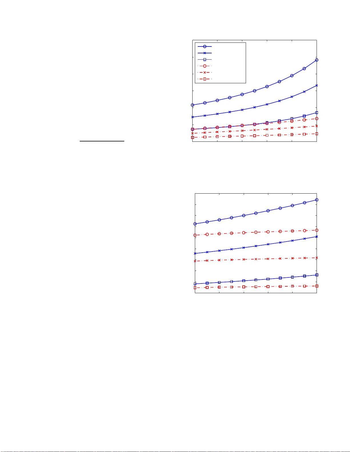
IEEE TRANSACTIONS ON INF ORMA TION THEOR Y 1 Rank Minimizat ion o v er Finite Fie lds: Fun damental Limits and Coding -Theoretic Inte rpretat ions V incent Y . F . T an, Laura Balzano, Student Membe r , IEEE , Stark C. Draper , Member , IEEE Abstract —This paper establ i shes info rmation-theoretic limits fo r estimating a ﬁnite ﬁeld low-rank matrix given rand om linear measureme nts of it. These linear m easurements a re o btained by tak i ng inner products of the low-rank matrix with random sensing matrices. Necessar y and sufﬁ cient conditions on the number of measureme nts required are provided. It is shown that these conditions are sh arp and the minimum-rank decoder is asymptotically optimal. Th e reliability functi on of this decoder is also derived by app ealing to d e Caen’ s lower bound on the probability of a union. The sufﬁcient condition also holds when the sensing matrices are sparse – a scenario that may be amenable to efﬁcient d ecodin g. More precisely , it is shown that if t h e n × n -sensing matrices contain, on av erage, Ω( n log n ) entries, the number of measurements required is the same as that when the sensing matrices ar e dense and contain entries drawn uni f ormly at random f rom the ﬁeld. Analogies are drawn b etween the ab ove results and rank-metric codes i n the coding th eory literature. In f act, we are also stro ngly motiv ated by u nderstanding wh en minimum rank dist an ce decoding of random rank-metric codes succeeds. T o this en d, we derive minimum distance pro perties of equiprobable and sparse rank-metric codes. Th ese distance properties provide a precise geo metric interpretation of the fact that the sparse ensemble requires as few measurements as t h e dense one. Index T erms —Rank minimization, Fi nite ﬁ elds, Reliabil i ty function, Sp arse p arity-check matrices, Rank-metric codes, Min- imum rank distance properties I . I N T RO D U C T I O N This p aper con siders the p roblem of ran k minimizatio n over ﬁnite ﬁelds. Our w ork attempts to con nect two seemingly dis- parate areas of study that have, by themselves, become popu lar in the inf ormation theor y comm unity in recent years: (i) th e theory of matrix completion [2]–[4] and rank minimization [5], [6] over the rea ls and ( ii) rank -metric codes [ 7]–[12], which are the ran k distance an alogs of binar y block codes en dowed with the Ham ming metric. T he work herein provid es a starting point for investigating the p otential impact of the low-rank assumption on inform ation and coding th eory . W e provide a brief review of th ese two areas of study . This work is supp orted in part by the Air Force Of ﬁce of Sci entiﬁc Research under grant F A9550-09-1-01 40 and by the National Scienc e Foundation under grant CCF 096383 4. V . Y . F . T an is also supported by A*ST AR Singapore. This paper was presented in part at the IEEE Internationa l Symposium on Information Theory (ISIT), St. Petersbur g, Russia, August 2011 [1]. The authors are with the Department of Electrical and Computer Engi- neering (ECE ), Unive rsity of W isconsin, Madison, WI, 53706, USA (emails: vtan@wisc .edu; sunbeam@ece.wisc.edu ; sdraper@ec e.wisc.edu). The ﬁrst author is also afﬁlia ted to the Laboratory for Informa tion and Decision Systems (LIDS), Massachusett s Institu te of T echnology (MIT), Cambridge, MA, 02139, USA (email: vtan@mit.edu). Copyri ght (c) 2011 IEEE . Personal use of this materi al is permit ted. Ho we ve r , permission to use this material for any other purposes must be obtaine d from the IEEE by sending a request to pubs-permissions@iee e.org. The problem of matrix completion [2]– [4] can be stated as follows: One is given a subset of no iseless o r n oisy entries of a low-rank matrix (with en tries ov er the reals), and is then required to estimate all the r emaining entries. T his pr oblem has a v ariety o f applications from collaborativ e ﬁltering (e.g., Netﬂix p rize [1 3]) to obtaining the minimal realizatio n of a linear dynam ical system [14]. Algorithms based on the n uclear norm (sum of sing ular values) con vex relaxation of th e rank function [14], [15] hav e enjoyed tremend ous successes. A generalizatio n of the matr ix c ompletion p roblem is the rank minimization p roblem [5], [6] where, instead of b eing g i ven entries of the low-rank matrix, one is given arb itrary linear measuremen ts of it. These linear measure ments are o btained by taking inner produ cts of the unkn own m atrix with sensing matrices. T he nuclear norm h euristic has also b een shown to be extremely effecti ve in estimating the unk nown low- rank matrix. Theor etical results [5], [6] are typ ically of the following ﬂa vour: If the numb er of measur ements (also known as the m easurement comp lexity) exceeds a small multiple of the product of the dimension of the m atrix and its r ank, then optim izing th e nuc lear-norm heur istic yields the same (optimal) solution as the rank minim ization problem und er certain conditio ns o n the sensing matrices. Note that in the case o f real matrices, if the o bservations (or the en tries) are noisy , p erfect reco nstruction is impossible. As we shall see in Section V, th is is not the case in th e ﬁnite ﬁeld setting . W e can r ecover the und erlying matrix e xactly a lbeit at the cost o f a high er measurement complexity . Rank-metric codes [7]–[ 12] are subsets of ﬁnite ﬁeld ma- trices endowed with the rank -metric. W e will be concerned with linear rank -metric codes, which may be chara cterized b y a family of pa rity-check matr ices, which are e quiv alent to the sensing matrices in th e rank minim ization problem. A. Motiva tions Besides analyzing the measurem ent complexity for rank minimization over ﬁnite ﬁelds, this paper is also m otiv a ted by two applications in coding . The ﬁrst is index codin g with side inf ormation [1 6]. In brief, a sender wants to comm unicate the l - th c oordina te of a leng th- L b it string to the l -th of L receivers. Furthermore, each of the L r eceiv ers knows a subset of the coordin ates of the bit string. T hese subsets can be represented b y (the ne ighbour hoods of ) a gr aph. Bar-Y ossef et al. [16] showed that th e linear versio n of this p roblem reduces to a r ank minimiza tion pr oblem. In previous works, the graph is d eterministic. Our work , and in particular the rank minimization pro blem co nsidered her ein, can be cast as IEEE TRANSACTIONS ON INFORMA TION THEOR Y 2 the solution of a linear index codin g problem with a rand o m side info rmation graph. Second, we are interested in p roperties of the r ank-metric coding proble m [10]. Here, we are given a set of matrix-valued codewords that fo rm a linea r rank- metric code C . A co dew ord C ∗ ∈ C is transmitted across a noisy ﬁnite ﬁeld matrix -valued channel which indu ces an additive err or matrix X . This error matrix X is a ssumed to be low rank. For example, X could be a matrix induced b y the crisscross error m odel in data arrays [17]. In the crisscro ss error mode l, X is a sparse low rank matrix in which the non- zero elements are restricted to a small nu mber of rows and colum ns. The received matr ix is R := C ∗ + X . T he minim um distan ce decod ing pro blem is giv en by the following: ˆ C := arg min C ∈ C rank( R − C ) . (1) W e would like to study wh en problem (1) succeeds ( i.e., uniquely recovers the true codeword C ∗ ) with high proba- bility 1 (w .h.p .) given that C is a rand om cod e c haracterized by either den se or sparse random par ity-check matrices and X is a determ inistic error matrix. But why analyze random codes? Our study of r andom (instead of determ inistic) codes is motiv ated by the fact tha t data arr ays that arise in applications are of ten corr upted by crisscross er ror pattern s [ 17]. Deco ding technique s used in the r ank-metr ic literature such as er ror trapping [11], [1 8] are u nfortu nately not a ble to correct such error pattern s because th ey are highly structured and hence the “er ror traps” would m iss (or not be able to cor rect) a non-tr i vial subset of error s. Indeed, the success such an erro r trapping strategy hing es strongly on the assumption th at the underly ing low-rank error matrix X is drawn un iformly at random over all matrices whose r ank is r [18, Sec. IV] (so subspaces can be trapped). Th e dec oding techniq ue in [17] is speciﬁc to correc ting crisscross error p atterns. In con trast, in this work, we ar e ab le to der i ve distanc e prop erties o f random rank-m etric co des and to show that given sufﬁciently many constraints on the codewords, a ll error patterns of ran k no gr eater than r can be successfully cor rected. A lthough our der i vations are similar in spirit to those in Barg and Forney [19], o ur startin g poin t is rather different. I n particu lar , we comb ine the u se of techniqu es from [ 20] and tho se in [19]. W e ar e also motivated by the fact th at error exponent- like results for matrix -valued ﬁnite ﬁeld ch annels ar e, to th e best of the author s’ knowledge, not a v ailable in the literature. Such channels have been popula rized by th e seminal work in [21]. Capacity resu lts for speciﬁc chan nel models such as the un iform given rank (u.g .r .) mu ltiplicativ e no ise mo del [2 2] have recently been derived. In this work, we derive the error exponent for the minimu m-rank decoder E ( R ) (fo r the addi- ti ve noise m odel). This ﬁlls an impor tant g ap in the literature. B. Main Con tributions W e summarize our fou r main contributions in this work. Firstly , by using a standar d converse technique ( Fano’ s inequality) , we deri ve a necessary condition on th e numb er 1 Here and in the follo wing, with hi gh probabi lity means with prob abili ty tending to one as the problem size tends to inﬁnity . of measureme nts requir ed f or estimating a lo w-rank matrix. Furthermo re, under the assumption that the linear measure- ments are obtained by taking inner pro ducts of the un known matrix with sensing matrices containing independ ent entries that are equipro bable ( in F q ), we demon strate an achievability proced ure, called the min-r ank decoder, that matches the informa tion-theor etic lower boun d on the n umber of m ea- surements r equired. Hence, the sufﬁcient condition is sharp. Extensions to the noisy case are also discussed. No te th at in this paper, we are not as concerned with the compu tational complexity of recovering the unk nown low-rank ma trix as compare d to the fundam ental limits of doin g so. Secondly , we d erive the reliab ility fun ction (err or expon ent) E ( R ) of the min-rank decod er by using de Caen’ s lo wer bound on the pr obability of a u nion [2 3]. The use of d e Caen’ s boun d to obta in estimates of the r eliability fu nction (or probability of erro r) is not new . See the works by S ´ eguin [24] and Co hen and Merhav [25] for example. Ho we ver , by exploiting pair wise indepen dence of constituent error events, we not on ly derive upper and lower bound s o n E ( R ) , we sho w that th ese boun ds are, in fact, tight for all rates (for the min -rank decode r). W e deri ve th e correspon ding err or exponents f or codes in [7] and [18] an d m ake co mparisons b etween the err or exp onents. Thirdly , we sho w that if the fraction of non -zero en tries of the sensing or measuremen t matrices scales ( on a verage) as Ω( log n n ) (where the matrix is of size n × n ), the m in-rank decoder ach ie ves the inform ation-theo retic lower bound . Thus, if the average nu mber of entries in each sparse sensin g m atrix is Ω( n log n ) (wh ich is much fewer than n 2 ), we can sho w that, very sur prisingly , the num ber o f linear measurem ents req uired for reliable reconstructio n of the unknown low-rank matrix is exactly the same as that for the equip robable (dense) case. This main result o f our s opens the po ssibility for the d e velopment of efﬁcient, message-passing decoding algorithms based on sparse parity-ch eck matrices [26]. Finally , we draw analog ies betwe en th e a bove results and rank-m etric cod es [7]–[12] in the coding theory literatur e. W e derive minim um (rank) distanc e prope rties of the equip robable random en semble and the spar se ran dom ensemble. Using elementary techniques, we derive an analog of the Gilbert- V arshamov distance fo r the r andom rank- metric cod e. W e also compare and co ntrast our result to classical bina ry linear block codes with the Ham ming metric [19]. From our analyses in this section, we ob tain g eometric in tuitions to explain why minimum r ank d ecoding perf orms we ll even when the sensing matrices are sparse. W e also use these geometr ic intuitions to guide ou r deriv ation of strong recovery guarantees alon g th e lines of the rec ent work by Eldar et al. [27]. C. Related W ork There is a wealth of literature on rank minimiza tion to which we will not be ab le to do justice here. See for example the seminal works by Fazel et al. [14], [15] and th e subsequ ent works b y o ther au thors [2]–[4] (a nd the ref erences ther ein). Howe ver , all these works focus on the case where the unknown matrix is ov er the reals. W e are inter ested in the ﬁnite ﬁeld setting becau se such a problem has ma ny connectio ns with IEEE TRANSACTIONS ON INFORMA TION THEOR Y 3 T ABLE I C O M PA R I S O N O F O U R W O R K ( T A N - B A L Z A N O - D R A P E R ) T O E X I S T I N G C O D I N G - T H E O R E T I C T E C H N I Q U E S F O R R A N K M I N I M I Z ATI O N Pape r Code Structure Decoding T ech nique Gabiduli n [7] Algebrai c Berleka mp-Masse y SKK [10] Algebrai c Extended Berlekamp-Ma ssey MU [11] Fact or Graph Error Trappi ng & Message Passing SKK [18] Error Trapping Error Trappi ng GLS [33] Perfect Graph Semideﬁnit e Program (Ellipsoid) TBD See T able II Min-Rank Decoder (Sectio n VIII) and ap plications to co ding and informa tion th eory [16], [17], [28]. The analogous prob lem for the reals was considered by Eldar et al. [27]. The r esults in [2 7], developed f or d ense sensing m atrices with i.i. d. Gaussian entries, mirr or those in this paper but only achie vability results (suf ﬁcient co nditions) are provided . W e add itionally analyze the sparse setting. Our work is partially in spired b y [29] where fun damental limits fo r comp ressed sensing over ﬁnite ﬁelds were deriv ed. T o the best o f our knowledge, V ishwanath’ s work [30] is the o nly one that employs info rmation-th eoretic techniq ues to derive nece ssary and sufﬁcient condition s on the n umber of measuremen ts required fo r reliab le matr ix completio n (or ran k minimization ). It was shown using ty picality argumen ts that the numb er of m easurements require d is with in a logarith mic factor of the lower boun d. Our setting is different becau se we assume that we have linear measur ements instead of rand omly sampled entries. W e are able to show that the achiev ability and con verse match for a family of rand om sensing m atrices. Emad a nd Milenkovic [31] recently exten ded the analyses in the conf erence version [1] of this pap er to the tensor case, where the rank , the order of the tensor and the num ber of measuremen ts grow simultaneou sly with the size of the matrix. W e co mpare and co ntrast o ur decoder a nd a nalysis for the noisy case to that in [3 1]. Another recen t r elated work is that by Kakhak i et al. [32] w here the auth ors co nsidered the bina ry erasure chan nel (BEC) and bina ry symmetric chann el (BSC) and empir ically studied the err or exponen ts for co des whose generator matrices are random and sparse. For the BEC, the authors sh owed that th ere exist capacity-ach ie ving c odes with generato r matrices whose sparsity factor (d ensity) is O ( log n n ) (similar to this work) . Howe ver , m otiv ated by the fact that sparse parity -check matrices may make d ecoding amenable to lower com plexity message-p assing type decoder s, we analyze the scenar io where the parity-check matrices are sparse. The family of cod es known as ran k-metric codes [ 7]–[12], which are the the rank-distan ce analog of binary block cod es equippe d with the Hamm ing metric, bears a striking similarity to the rank minimization problem over ﬁnite ﬁelds. Compar- isons between this w ork and related works in the coding theory literature are summarized in T able I. Our con tributions in th e various sections of this pape r , and o ther pe rtinent referen ces, are summ arized in T able I I. W e will fur ther elabor ate on these compariso ns in Section IX-A. D. Outline o f P aper Section I I details our n otational choices, describes the measuremen t models and states the p roblem. In Section III, we T ABLE II C O M PA R I S O N S B E T W E E N T H E R E S U LT S I N V A R I O U S S E C T I O N S O F T H I S PA P E R A N D OT H E R R E L ATE D W O R K S Parit y-chec k Random Det erminist ic matrix H a lo w-rank m atrix X lo w-rank matrix X Random, dense Section IV Sectio n IV Determini stic, dense Sec tion IV, [18] Section VII-C, [7], [10] Random, sparse Section VI Sectio n VI Determini stic, sparse Section VI, [11], [18] Sect ion VII-C use Fano’ s inequ ality to derive a lower boun d on the number of measurements for reconstructing the un known low-rank matrix. In Section IV, we co nsider the u niformly a t ran dom (or equip robable) mo del wh ere th e entries o f the measurem ent matrices are selected indepen dently and uniform ly at random from F q . W e derive a su fﬁcient co ndition fo r reliable recovery and th e reliab ility f unction of the min-ran k decode r using de Caen’ s lower boun d. The results are then extended to the n oisy scenario in Section V. Section VI, which conta ins ou r main result, considers the case wher e the mea surement matrices a re sparse. W e deriv e a su fﬁcient co ndition on the sparsity factor (density) as well as the number o f measur ements for r eliable recovery . Section VII is devoted to u nderstand ing and inter - preting the ab ove results from a cod ing-theo retic perspec ti ve. In Sectio n VIII, we provid e a pro cedure to sear ch fo r the low-rank ma trix by exploiting ind eterminacies in the p roblem. Discussions and conclusion s ar e provided in Section IX. The lengthier proo fs are deferred to the app endices. I I . P RO B L E M S E T U P A N D M O D E L In this section, we state our notatio nal conventions, describe the system mo del and state the p roblem. W e also disting uish between the two related no tions o f weak and strong recovery . A. Notatio n In this paper we a dopt the following set of no tations: Serif font and san-serif fon t denote deterministic and random quantities r espectiv ely . Bold -face upp er-case and b old-face lower -case denote m atrices and ( column) vectors r espectiv ely . Thus, y , y , X and X den ote a determ inistic scalar, a scala r- valued r andom variable, a determ inistic matrix an d a rand om matrix respectively . Random func tions will a lso be den oted in san-serif font. Sets (and e vents) a re denoted with calligraphic font ( e.g., U or C ). The cardinality of a ﬁnite set U is denoted as |U | . For a prime power q , we denote the ﬁnite (Galois) ﬁeld with q elements as F q . If q is prime, one can identify F q with Z q = { 0 , . . . , q − 1 } , the set of th e integers modulo q . The set of m × n matrices with e ntries in F q is denoted as F m × n q . For simplicity , we let [ k ] := { 1 , . . . , k } and y k := ( y 1 , . . . , y k ) . For a matrix M , the notation s k M k 0 and rank( M ) respectively d enote the num ber of non -zero elements in M (the Hamm ing weigh t) and the r ank of M in F q . For a matrix M ∈ F m × n q , we also use the no tation vec ( M ) ∈ F mn q to d enote vectorizatio n of M with its c olumns stacked on top of one another . For a real numb er b , the notation | b | + is deﬁned as max { b , 0 } . Asymptotic notation such as O ( · ) , Ω( · ) and o ( · ) will be used through out. See [34, IEEE TRANSACTIONS ON INFORMA TION THEOR Y 4 T ABLE III T AB L E O F S Y M B O L S U S E D I N T H I S PA P E R Notatio n Deﬁnitio n Section k Number of measurement s Section II-B r /n → γ Rank-dime nsion ratio Section II-B σ = k w k 0 /n 2 Determini stic noise paramete r Section V -A α = k/n 2 Measurement scaling parameter Section V -B p = E k w k 0 /k Random noise parameter Section V -B δ = E k H a k 0 /n 2 Sparsity factor Section VI N C ( r ) Num. of matrices of rank r in C Section VII d ( C ) Minimum rank distance of C Section VII Sec. I. 3] f or d eﬁnitions. For the reade r’ s co n venience, we have summarized the symb ols used in this p aper in T able III. B. System Model W e are interested in the following model: Let X b e a n unknown (determ inistic o r r andom) squ are 2 matrix in F n × n q whose rank is less than or equal to r , i.e., rank( X ) ≤ r . T he upper bou nd on the rank r is allowed to be a fun ction of n , i.e., r = r n . W e assum e that r /n → γ and we say th at the limit γ ∈ [0 , 1] is the rank-dimen sion ratio . 3 W e would like to recover or estimate X fr om k linear measur ements y a = h H a , X i := X ( i,j ) ∈ [ n ] 2 [ H a ] i,j [ X ] i,j a ∈ [ k ] , (2) i.e., y a is the trace of H a X T . In (2), the sensing or mea- sur ement matrices H a ∈ F n × n q , a ∈ [ k ] , are ra ndom matrices chosen according to som e probability m ass function ( pmf). The k scalar measur ements y a ∈ F q , a ∈ [ k ] , are av ailable for estimating X . W e will o perate in the so- called high- dimensiona l setting and allow the numbe r o f measurem ents k to depend o n n , i.e., k = k n . M ultiplication and ad dition in (2) a re perf ormed in F q . I n the subseque nt sections, we will also be interested in a gener alization of the m odel in ( 2) where the measu rements y a , a ∈ [ k ] , may not be n oiseless, i.e., y a = h H a , X i + w a , a ∈ [ k ] , (3) where w a , a ∈ [ k ] , rep resents rando m o r determ inistic noise. W e will specify pre cise noise models in Section V. The measure ment m odels we are concern ed with in this paper, (2) and ( 3), are somewhat different from the matrix completion pr oblem [ 2]–[4]. In the matrix c ompletion setup , a subset o f entries Ω ⊂ [ n ] 2 in the matrix X is observed and one would like to “ﬁll in” the r est of the entries assumin g the matrix is low-rank. T his model can be captured by (2) by choosing each sensing matrix H a to b e no n-zero only in a single position. Assuming H a 6 = H a ′ for all a 6 = a ′ , the num- ber of m easurements is k = | Ω | . In contra st, o ur measu rement models in (2) and (3) do not assume that k H a k 0 = 1 . The sensing matrices a re, in genera l, dense althou gh in Section VI, 2 Our result s are not restricte d to the case where X is square but for the most part in this paper , we assume that X is square for ease of expositi on. 3 Our results also inclu de the regime where r = o ( n ) b ut the case where r = Θ( n ) (and γ is the proportio nalit y constant) is of greate r interest and signiﬁca nce. T his is because the rank r grows as rapidly as possible and hence this re gime is the most chall enging. Note that if r /n → γ = 1 , then we would need n 2 measurement s to recov er X since we are not making any low rank assumptions on it. This is corrobora ted by the con verse in Proposition 2. we also analyze the scenario wh ere H a is relativ ely sparse. Our setting is more similar in spirit to the rank minim ization problem s analyzed in Recht et al. [5], Meka et al. [6] and Eldar et al. [27]. Howe ver , these works focus on p roblems in the reals wher eas our focus is the ﬁnite ﬁeld setting. C. Pr oblem Statemen t Our objective is to estimate the unk nown low-rank m atrix X given y k (and the measurem ent matrices H a , a ∈ [ k ] ). I n general, giv en the measureme nt mod el in (2) and without any assumption s o n X , the p roblem is ill-posed an d it is not possible to recover X if k < n 2 . Howe ver , because X is a ssumed to have rank n o larger than r ( and r /n → γ ), we can exploit this addition al in formation to estimate X with k < n 2 measuremen ts. Our goal in this paper is to characterize nece ssary and sufﬁcient conditio ns on the n umber of measurem ents k as n becomes large assuming a particular pmf g overning the sensing m atrices H a , a ∈ [ k ] and under various ( random and determin istic) models on X . D. W eak V ersus Str o n g Recovery In this paper, we will focus (in Sections I II to VI) on the so-called weak recovery p roblem where the un known low-rank matrix X is ﬁ xed and we ask how many measurements k are sufﬁcient to r ecover X (and w hat the proced ure is f or doing so). Ho wev er , ther e is also a companio n pro blem kn own as the str on g recovery pro blem, where o ne would like to recover all matrices in F n × n q with rank no larger than r . A familiar version o f this distinction also arises in compr essed sensing . 4 More precisely , given k sensing matr ices H a , a ∈ [ k ] , we deﬁne the linear o perator H : F n × n q → F k q as H ( X ) := [ h H 1 , X i , h H 2 , X i , . . . , h H k , X i ] T . (4) Then, a necessary and sufﬁcient con dition for strong recovery is that the op erator H is in jecti ve when restricted to the set of all matr ices of rank- 2 r (or less). In other words, there are no rank - 2 r ( or less) ma trices in th e nullspace of the op erator H [27, Sec. 2]. This can be ob served b y noting that for two matrices X 1 and X 2 of ran k- r (or less) that g enerate the same linear observations (i.e., H ( X 1 ) = H ( X 2 ) ), their difference X 1 − X 2 has rank at most 2 r by the triangle inequ ality . 5 W e would th us like to ﬁnd condition s on k (via, for example, the geometry of the random cod e) such that the fo llowing sub set of F n × n q R ( n ) 2 r := { X ∈ F n × n q : rank( X ) ≤ 2 r } (5) is disjoint from the nullspac e of H with pr obability tend ing to one as n g rows. As mentioned in Section II-B, we allow r to 4 Analogousl y in compressed sensi ng, consider the combinatorial ℓ 0 -norm optimiza tion problem min ˜ x ∈ F n {k ˜ x k 0 : A ˜ x = y } , where the ﬁeld F can eithe r be the real s R [27] or a ﬁnite ﬁeld F q [29]. It can be seen that if we want to recov er ﬁxed but unknown s -sparse vector x (weak reco ve ry), s + 1 linear measurements sufﬁc e w .h.p. Howe ve r , for strong reco very where we would like to guarante e recov ery for all s -sparse vect ors, we need to ensure that the nul lspace of the measurement matrix A is disjoint from the set of 2 s -sparse v ectors. Thus, w .h. p., 2 s measurement s are required for strong reco very [27], [29]. 5 Note that ( A , B ) 7→ rank( A − B ) is a m etric on the space of matrices. IEEE TRANSACTIONS ON INFORMA TION THEOR Y 5 grow linearly with n (with prop ortionality constant γ ) . Under the condition that R ( n ) 2 r ∩ n ullspace( H ) = ∅ , the solution to the rank minimization p roblem [ stated pr ecisely in (12) below] is unique an d corr ect for all low-rank matrices w ith p robability tending to one as n grows. As we shall see in Section VII-C, the conditio ns on k fo r strong recovery are more stringent than th ose f or weak recovery . See the recen t p aper b y Eldar et al. [27, Sec. 2] for f urther discussions on weak versus strong recovery in the real ﬁeld setting . E. Bo unds on the nu mber of low-rank matrices In the seq uel, we will ﬁnd it usefu l to leverage the fo llowing lemma, which is a combina tion of results stated in [2 1, Lemma 4], [ 9, Proposition 1] and [12, Lemma 5]. Lemma 1 (Bounds o n the number of low-rank matrices) . Let Φ q ( n, r ) and Ψ q ( n, r ) r espe c tively be the number o f matrices in F n × n q of rank exactly r and the number of matrices in F n × n q of rank less than or equ a l to r . Note that Ψ q ( n, r ) = P r l =0 Φ q ( n, l ) . The following bou nds h old: q (2 n − 2) r − r 2 ≤ Φ q ( n, r ) ≤ 4 q 2 nr − r 2 , (6) q 2 nr − r 2 ≤ Ψ q ( n, r ) ≤ 4 q 2 nr − r 2 . (7) In oth er word s, we have fro m (7) and the fact that r /n → γ that | 1 n 2 log q Ψ q ( n, r ) − 2 γ (1 − γ / 2 ) | → 0 . I I I . A N E C E S S A RY C O N D I T I O N F O R R E C O V E RY This section p resents a necessary conditio n on the scaling of k with n for the matrix X to b e recovered r eliably , i.e., fo r the error probability in estimating X to tend to zero as n g rows. As with most other conv erse statements in informa tion theo ry , it is necessary to assume a statistical model on the unk nown o bject, in this case X . Hence, in this section, we denote the unkn own low-rank matrix as X (a rand om variable). W e a lso assume that X is drawn uniformly at random fro m th e set of m atrices in F n × n q of rank less th an or eq ual to r . For an estimator (determin istic or ra ndom f unction) ˆ X : F k q × ( F n × n q ) k → F n × n q whose range is the set o f all F n × n q -matrices whose rank is less than or equ al to r , we de ﬁne the erro r e vent: ˜ E n := { ˆ X ( y k , H k ) 6 = X } . (8) This is the event that the estimate ˆ X ( y k , H k ) is not equal to th e true low-rank matrix X . W e emphasize that the estimator can either b e determin istic or ra ndom. In a ddition, the argumen ts ( y k , H k ) are rando m so ˆ X ( y k , H k ) in the d eﬁnition of ˜ E n is a random matrix . W e can demon strate the following: Proposition 2 (Con verse) . Fix ε > 0 an d assume that X is drawn uniformly at random fr om all matrices of rank less than or equa l to r . Also, assume X is indepen dent of H k . If, k < (2 − ε ) γ (1 − γ / 2) n 2 (9) then for an y estimator ˆ X whose range is the set o f F n × n q - matrices whose rank is less than or eq ual to r , P ( ˜ E n ) ≥ ε/ 4 > 0 for a ll n sufﬁciently lar ge. Proposition 2 states that the n umber of me asurements k must exceed 2 n r − r 2 (which is a pproxim ately 2 γ (1 − γ / 2) n 2 ) for rec overy o f X to be r eliable , i. e., f or the probability of ˜ E n to tend to zero as n grows. From a linea r algebraic perspective, this m eans we need at least as many measur ements as there are degrees of freedom in the unkn own object X . Clearly , the bound in (9) applies to both the no isy and the noiseless mod els introdu ced in Section II-B. The p roof in volves an elem entary application of Fano’ s ineq uality [35, Sec. 2 .10]. Pr oo f: Con sider the following lower bo unds o n th e p rob- ability of erro r P ( ˜ E n ) : P ( ˆ X 6 = X ) ( a ) ≥ H ( X | y k , H k ) − 1 log q Ψ q ( n, r ) = H ( X ) − I ( X ; y k , H k ) − 1 log q Ψ q ( n, r ) ( b ) = H ( X ) − I ( X ; y k | H k ) − 1 log q Ψ q ( n, r ) = H ( X ) − H ( y k | H k ) − 1 log q Ψ q ( n, r ) ( c ) ≥ H ( X ) − k − 1 log q Ψ q ( n, r ) ( d ) = 1 − k log q Ψ q ( n, r ) − o (1) , (10) where ( a ) is by Fano’ s inequality (estimating X giv en y k and H k ), ( b ) is bec ause H k is in depende nt of X so I ( X ; y k , H k ) = I ( X ; y k | H k ) + I ( X ; H k ) = I ( X ; y k | H k ) . Inequality ( c ) is due to the fact that y a is q -ary f or all a ∈ [ k ] so H ( y k | H k ) ≤ H ( y k ) ≤ k H ( y 1 ) ≤ k log q q = k , (11) and ﬁnally , ( d ) is due to th e u niformity of X . It can be easily veriﬁed th at if k satisﬁes (9) for some ε > 0 , then k / log q Ψ q ( n, r ) ≤ 1 − ε/ 3 for n sufﬁciently large by th e lower bound in (7) and the conver gence r/n → γ . Hence, (10) is larger than ε/ 4 for all n sufﬁciently large. W e emp hasize th at th e assum ption that th e sensing matrices H a , a ∈ [ k ] a re statistically independen t of the unk nown low- rank matrix X is importan t. T his is to ensure the validity of equality ( b ) in (10). T his a ssumption is not a r estrictiv e o ne in practice since the sensing m echanism is usually ind ependen t of the u nknown matrix. I V . U N I F O R M LY R A N D O M S E N S I N G M A T R I C E S : T H E N O I S E L E S S C A S E In this section, we assume the noiseless linear m odel in (2) and p rovide su fﬁcient co nditions for the rec overy of a ﬁ xed X (a determ inistic low-rank matrix) given y k , where r ank( X ) ≤ r . W e will also provide the functio nal form of the reliab ility function (error e xponen t) for this recovery problem . T o do so we ﬁrst con sider the following optimization problem: minimize rank( ˜ X ) sub ject to h H a , ˜ X i = y a , a ∈ [ k ] ( 12) The optimiza tion variable is ˜ X ∈ F n × n q . Thus amon g a ll the matrices th at satisfy the lin ear con straints in (2), we select o ne whose rank is the smallest. W e call the optimization problem in (12) the min -rank decoder , den oting the set of m inimizers as S ⊂ F n × n q . If S is a singleton set, we also denote the unique optimizer to ( 12), a random qua ntity , as X ∗ . W e analyze the error pr obability that e ither S is n ot a sing leton set or X ∗ does not equal the tru e matrix X , i.e., the error event E n := {|S | > 1 } ∪ ( { |S | = 1 } ∩ { X ∗ 6 = X } ) . (13) IEEE TRANSACTIONS ON INFORMA TION THEOR Y 6 The optimiz ation in (12) is, in general, intractab le (in fact NP-hard) unless ther e is additiona l structu re on the sensing matrices H a (See discussions in Section I X). Our focu s, in this paper, is o n the infor mation-theo retic limits f or solvin g (12) and its variants. W e remark that the minimizatio n pr oblem is reminiscen t of Csisz ´ ar’ s so-called α -deco der fo r line ar codes [3 6]. In [3 6], Csisz ´ ar analyzed the e rror exponen t of the decode r that minimizes a function α ( · ) [e.g ., the en tropy H ( · ) ] of the typ e (or empirical distribution) of a sequ ence subject to the seq uence satisfying a set of linear con straints. For this section and Section V, we assume that each element in each sensing matrix is drawn ind ependen tly and unifor mly at rand om from F q , i.e., fro m the pmf P h ( h ; q ) = 1 /q , ∀ h ∈ F q . (14) W e ca ll this the uniform or equip r obable mea surement model. For simplicity , througho ut th is section, we use the notation P to denote th e pr obability m easure associated to the equipr obable measuremen t model. A. A Sufﬁcient Con dition for Rec overy in the Noiseless Case In this subsectio n, we assume the noiseless lin ear m odel in (2). W e can no w exploit ideas from [29] to demonstrate the f ollowing achievability (weak recovery) result. Recall that X is non- random and ﬁxed, a nd w e are askin g how many measuremen ts y 1 , . . . , y k are sufﬁcient for recovering X . Proposition 3 (Ach iev ab ility) . F ix ε > 0 . Under the u niform measur ement model as in ( 14) , if k > (2 + ε ) γ (1 − γ / 2) n 2 (15) then P ( E n ) → 0 as n → ∞ . Note that the number o f measur ements stipu lated by Propo - sition 3 ma tches the info rmation- theoretic lower bou nd in (9). In this sense, the min-rank decoder prescribed by the optimiza- tion p roblem in (1 2) is asym ptotically optimal, i.e., the b ounds are sharp . Note also that in the con verse (Proposition 2), the range of the dec oder ˆ X ( · ) is co nstrained to b e the set of matrices whose rank does no t exceed r . He nce, the decod er in the con verse has addition al side infor mation – namely the upper bou nd on the r ank. For th e min- rank de coder in (1 2), no such k nowledge of the ran k is requ ired and yet it m eets the lower bound. W e r emark that the pack ing-like achie vability proof is much simp ler than the typ icality-based argum ent presented by V ishwanath in [ 30] (albeit in a d ifferent setting ). Pr oo f: T o each matr ix Z ∈ F n × n q that is no t equal to X and whose ran k is no grea ter than rank( X ) , deﬁne th e event A Z := {h Z , H a i = h X , H a i , ∀ a ∈ [ k ] } . ( 16) Then we n ote that P ( E n ) = P   [ Z : Z 6 = X , rank( Z ) ≤ rank( X ) A Z   (17) since an error occurs if and only if there exists a matrix Z 6 = X such tha t (i) Z satisﬁes th e linear constrain ts, (ii) its rank is less than or equ al to the rank o f X . Furtherm ore, we claim that P ( A Z ) = q − k for ev ery Z 6 = X . This follows b ecause P ( A Z ) = P ( h Z − X , H a i = 0 , a ∈ [ k ]) ( a ) = P ( h Z − X , H 1 i = 0 ) k ( b ) = q − k , (18) where ( a ) fo llows from the fact that the H a are i.i.d. matrices and ( b ) from the fact Z − X 6 = 0 and every no n-zero element in a ﬁn ite ﬁeld has a (un ique) m ultiplicative in verse so P ( h Z − X , H 1 i = 0 ) = q − 1 [29], [3 6]. More precisely , this is because h Z − X , H 1 i has distribution P h by ind ependen ce and unifo rmity of th e elements in H 1 . Since r/n → γ , for any ﬁxed η ′ > 0 , | r/ n − γ | ≤ η ′ for all n sufﬁciently large. By the unifor m continuity of the function t 7→ 2 t − t 2 on t ∈ [0 , 1] , for any η > 0 , | (2 nr − r 2 ) /n 2 − 2 γ (1 − γ / 2) | ≤ η for all n ≥ N η (an integer just depen ding on η ). Now by com bining ( 18) with the union of e vents bound, P ( E n ) ≤ X Z : Z 6 = X , rank( Z ) ≤ rank( X ) q − k ( c ) ≤ Ψ q ( n, r ) q − k ( d ) ≤ 4 q 2 nr − r 2 − k ( e ) ≤ 4 q − n 2 [ − 2 γ ( 1 − γ / 2) − η + k/n 2 ] , (19) where ( c ) fo llows becau se rank( X ) ≤ r , ( d ) follows fr om the up per bou nd in (7) an d ( e ) fo llows f or all n su fﬁciently large as argued ab ove. Thus, we see that if k satisﬁes (15), th e exponent in (19) is positi ve if we ch oose η ′ sufﬁciently small so that η < ε γ (1 − γ / 2) . Hence P ( E n ) → 0 as desired. Remark: Her e an d in the following, we can, without loss of g enerality , assume that r = ⌊ γ n ⌋ (in p lace of r/ n → γ ) . In this way , we can rem ove the effect of th e small po siti ve constant η as in the above argum ent. This simpliﬁcation does not affect the precision o f any of the argum ents in the sequ el. B. The Relia bility Function W e have shown in the p revious section that the min-ran k decoder is asymptotica lly optimal in the sense th at the nu mber of measurements required fo r it to decod e X reliably with P ( E n ) → 0 m atches the lower boun d (n ecessary condition ) on k (Pr oposition 2). It is also interesting to a nalyze the rate of decay of P ( E n ) for th e min-rank decoder . For this purp ose, we deﬁne the r ate R of the measuremen t model. Deﬁnition 1. The rate of ( a seque nce o f) linea r me asur ement models as in (2) is deﬁn ed as R := lim n →∞ n 2 − k n 2 = lim n →∞ 1 − k n 2 (20) assuming the limit exists. Note th at R ∈ [0 , 1] . The use o f the term rate is in direct analog y to the use o f the term in co ding theory . Th e rate of the line ar code C := { C ∈ F n × n q : h C , H a i = 0 , a ∈ [ k ] } (21) is R n := 1 − dim(span { vec( H 1 ) , . . . , vec( H k ) } ) /n 2 , which is lo wer bou nded 6 by 1 − k /n 2 for every k = 0 , 1 , . . . , n 2 . 6 The lo wer bound is achie ved when the vect ors ve c( H 1 ) , . . . , vec( H k ) are linea rly independent in F q . See Section VII, and in partic ular Proposition 14, for detail s when the sensing matrices are random. IEEE TRANSACTIONS ON INFORMA TION THEOR Y 7 W e r evisit the co nnection o f the ran k minimization pro blem to coding theory (a nd in particular to ran k-metric c odes) in detail in Section VI I. Deﬁnition 2. If the limit exists, th e reliability func tion or er ror exponent of the min-rank decoder (12) is d eﬁned as E ( R ) := lim n →∞ − 1 n 2 log q P ( E n ) . (22) W e show in Corollary 7 that the lim it in (22) indeed exists. Unlike the usual deﬁnition of the re liability function [3 7, Eq. (5.8.8 )], the normalization in (22) is 1 /n 2 since X is an n × n matrix. 7 Also, we restrict o ur atten tion to the min -rank decoder . The f ollowing pr oposition provides an upp er bound on the reliability functio n of the min- rank d ecoder wh en th ere is no n oise in the measu rements as in (2). Proposition 4 ( Upper bound on E ( R ) ) . Assume tha t rank( X ) /n → ˜ γ a s n → ∞ . Un der th e uniform measurement model in ( 14) and assuming the min-rank decoder is used, E ( R ) ≤ | (1 − R ) − 2 ˜ γ (1 − ˜ γ / 2) | + . (23) The proof of this result hing es on the pairwise ind ependen c e of the events A Z and de Caen’ s inequality [23], which fo r the reader’ s con venien ce, we r estate here: Lemma 5 (de Caen [23]) . Let (Ω , F , Q ) be a pr obability space. F or a ﬁnite n umber events B 1 , . . . , B M ∈ F , the pr ob ability of their un ion can be lower bounded as Q M [ m =1 B m ! ≥ M X m =1 Q ( B m ) 2 P M m ′ =1 Q ( B m ∩ B m ′ ) . (2 4) W e now prove Proposition 4. Pr oo f: In order to apply (24) to analyze the error proba- bility in (17), we need to compute the p robabilities P ( A Z ) an d P ( A Z ∩ A Z ′ ) . Th e former is q − k as argued in (18). The latter uses the f ollowing lemma wh ich is proved in Append ix A. Lemma 6 (Pairwise Indep endence) . F or any two distinct matrices Z and Z ′ , neither of which is equ a l to X , the events A Z and A Z ′ (deﬁne d in (1 6) ) ar e indepen d ent. As a result of this lemma, P ( A Z ∩ A Z ′ ) = P ( A Z ) P ( A Z ′ ) = q − 2 k if Z 6 = Z ′ and P ( A Z ∩ A Z ′ ) = P ( A Z ) = q − k if Z = Z ′ . Now , we apply the lo wer bound (24) to P ( E n ) noting from (17) that E n is the union of all A Z such that Z 6 = X and ra nk( Z ) ≤ ˜ r := rank( X ) . Then, for a ﬁxed η > 0 , we have P ( E n ) ≥ X Z : Z 6 = X rank( Z ) ≤ rank( X ) q − 2 k q − k 1 + P Z ′ : Z ′ 6 = X , Z rank( Z ′ ) ≤ rank( X ) q − k ! ( a ) ≥ ( q 2 n ˜ r − ˜ r 2 − 1) q − k 1 + 4 q 2 n ˜ r − ˜ r 2 − k ( b ) ≥ q n 2 [2 ˜ γ (1 − ˜ γ / 2) − η − k/n 2 ] − q − k 1 + 4 q n 2 [2 ˜ γ (1 − ˜ γ / 2)+ η − k/n 2 ] , where ( a ) is fro m the upper and lower b ounds in (7) and ( b ) h olds fo r all n sufﬁciently large since ˜ r /n → ˜ γ . See argument justifying inequality ( c ) in ( 19). Assum ing that 7 The “block-leng th” of the code C in (21) is n 2 . 1 − R > 2 ˜ γ ( 1 − ˜ γ / 2) , the n ormalized logarith m of the error probab ility can now be simpliﬁed as lim sup n →∞ − 1 n 2 log q P ( E n ) ≤ − 2 ˜ γ (1 − ˜ γ / 2 ) + η + lim n →∞ k n 2 , (25) where we used the fact that 4 q n 2 [2 ˜ γ (1 − ˜ γ / 2)+ η − k/n 2 ] → 0 f or sufﬁciently small η > 0 . The case where 1 − R ≤ 2 ˜ γ (1 − ˜ γ / 2) results in E ( R ) = 0 because P ( E n ) fails to conver ge to z ero as n → ∞ . The pro of of th e upp er b ound o f the r eliability function is c ompleted by ap pealing to the deﬁnition of R in (20) and the arbitrariness of η > 0 . Corollary 7 ( Reliability function) . Under the assumption s of Pr op osition 4, the err o r exponent of the min - rank d ecoder is E ( R ) = | (1 − R ) − 2 ˜ γ (1 − ˜ γ / 2) | + . (26) Pr oo f: Th e lower bou nd on E ( R ) follows fro m the achiev ability in (19), which may be strengthened as follows: P ( E n ) ≤ 4 q − n 2 | − 2 ˜ γ (1 − ˜ γ / 2) − η + k/n 2 | + , (27) since P ( E n ) can also be upp er bounded by unity . Now , because | · | + is continuous, the lo wer li mit of the normalized logarithm of the b ound in (27) can be expressed as follows: lim inf n →∞ − 1 n 2 log q P ( E n ) ≥     − 2 ˜ γ (1 − ˜ γ / 2) − η + lim n →∞ k n 2     + . (28) Combining th e upper bound in Propo sition 4 and the lower bound in ( 28) and noting that η > 0 is a rbitrary yields the reliability fun ction in (26). W e observe that pairwise indepen dence o f the events A Z (Lemma 6) is essential in the pr oof o f Propo sition 4. Pairwise indepen dence is a conseque nce of the linear measure ment model in (2) an d the un iformity assump tion in (14). No te that the e vents A Z are not jointly (nor triple- wise) indepe ndent. But the beauty of de Caen’ s bo und allo ws us to exploit the pairwise indepen dence to lower boun d P ( E n ) and thus to obtain a tight u pper bound o n E ( R ) . T o dr aw an analogy , just as only pairwise ind ependen ce is required to show that linear codes achieve capacity in symmetric DMCs, de Caen’ s inequality allows us to m ove the exploitation of pairwise indepen dence into the error expon ent domain to m ake statements abo ut the error exponent behavior of ensembles of line ar codes. A natu ral question arises: Is E ( R ) given in (26) th e largest possible expon ent over all deco ders ˆ X ( · ) for th e mo del in which H a follows the u niform pmf ? W e conjectu re that this is indeed the ca se, but a proof remain s elusi ve. 1) Comparison of err or exponen ts to exist ing works [38]: As mentioned in th e Introduc tion, the preced ing results can be interpreted fro m a cod ing-theor etic persp ecti ve. Th is is indeed wh at we will do in Section VII. In th is su bsection, we compare th e r eliability fu nction der i ved in Corollary 7 with three other coding techniques presen t in the literature . First, we ha ve the well-known construc tion of maximum rank distance ( MRD) co des by Gabidu lin [7]. Secon d, we have the error trapp ing tech nique [18] alluded to in Section I-A. Third, we hav e a co mbination of the two preced ing code IEEE TRANSACTIONS ON INFORMA TION THEOR Y 8 construction s which is discussed in [1 8, Section VI.E]. T o perfor m this comparison, we deﬁne another reliability function E 1 ( R ) that is “normalized by n ”. This is simply the quantity in (22) wh ere the no rmalization is 1 /n instead of 1 /n 2 . W e now denote the reliability functio n normalized by n 2 as in ( 22) by E 2 ( R ) . W e also use various superscripts o n E 1 and E 2 to denote different coding schem es. Hen ce, f or our encoding and decod ing strategy u sing random sensing and min- rank decodin g (RSMR), E RSMR 1 ( R ) = ∞ f or all R ≤ (1 − γ ) 2 and E RSMR 2 ( R ) is giv en by (26). Since Gab idulin co des are MRD, they ach iev e the Sin gleton bound [12, Section III] ) for rank-me tric cod es giv en by n 2 − k ≤ n ( n − d R + 1) , where d R is the minimum ran k distance of the code in (2 1) [See exact d eﬁnitions in ( 48) and (4 9)]. Thus, it can b e veriﬁed that for j = 1 , 2 , E Gab j ( R ) =  ∞ R ≤ 1 − 2 γ 0 else . (29) From [1 8, Section IV .B, Eq. (12)], it can also be checked that for th e error trapping cod ing strategy , assuming the low-rank error matrix is uniform ly distributed over th ose of ran k r , E ET 1 ( R ) =    1 − γ − √ R    + , E ET 2 ( R ) = 0 . (30) Finally , fr om [18, Section VI.E], f or the combina tion of Gabidulin codin g and er ror trap ping, und er the same con dition of unifo rmity , E GabET 1 ( R ) =     1 − γ − R 1 − γ     + , E GabET 2 ( R ) = 0 . (31) Note that for the error expone nts in ( 29), ( 30) and ( 31), the random ness is over the low-rank er ror matrix X and not th e code c onstruction , whic h is deterministic . In con trast, our coding strategy RSMR inv olves a random en coding scheme. It can be seen fr om (29) to (31) that there is a non- trivial interval of rates R := [1 − 2 γ , (1 − γ ) 2 ] in which our reliability function s E RSMR 1 ( R ) and E RSMR 2 ( R ) are th e best (largest). Indeed, in the inter val R , E RSMR 1 ( R ) = ∞ an d our result in (2 2) implies that E RSMR 2 ( R ) > 0 whereas all the abovemen tioned codin g schemes g i ve E 2 ( R ) = 0 . Thu s, using both a rando m code fo r encoding and min-rank decoding is advantageo us from a reliability fu nction stan dpoint in the regime R ∈ R . Fu rthermor e, as we shall see f rom (40) in Section VI which deals with the sparse sensing setting (SRSMR), E SRSMR 1 ( R ) = ∞ and E SRSMR 2 ( R ) = 0 for all R ≤ (1 − γ ) 2 . Such an encod ing scheme using sparse parity-ch eck matrice s may be amen able for the design o f low-complexity decoding strategies that also have good error exponent p roperties. I n general though, ou r min -rank decoder requires exhaustive sear ch (th ough Sectio n VIII pro poses technique s to redu ce the searc h space) , while all the preceding technique s h av e polynom ial-time d ecoding complexity . V . U N I F O R M LY R A N D O M S E N S I N G M AT R I C E S : T H E N O I S Y C A S E W e now gener alize the no iseless mo del and the accomp any- ing results in Section I V to the case where th e measurements y k are noisy as in (3). As in Sectio n IV, we assume that th e elements of H a are i.i.d. and unif orm in F q . The noise w is ﬁrst assumed in Section V -A to be deterministic but unknown. W e then extend our results to the situatio n where w is a rando m vector in Section V -B . A. Deterministic Noise In the deterministic setting, we assume that k w k 0 = ⌊ σ n 2 ⌋ for some noise level σ ∈ (0 , k / n 2 ] . Instead of using the minimum entropy d ecoder as in [29] (also see [36]), we consider th e fo llowing generalization of the min -rank deco der: minimize rank( ˜ X ) + λ k ˜ w k 0 sub ject to h H a , ˜ X i + ˜ w a = y a , a ∈ [ k ] (32) The optimiza tion v ariables are ˜ X ∈ F n × n q and ˜ w ∈ F k q . The parameter λ = λ n > 0 governs th e tradeo ff between th e rank of the matrix X and the sparsity of the vector w . L et H q ( p ) := − p log q ( p ) − (1 − p ) log q ( p ) be th e (base- q ) bin ary entropy . Proposition 8 (Achiev ability un der deterministic noisy me a- surement model) . F ix ε > 0 and choose λ = 1 /n . Assume the uniform measurement mod el and that k w k 0 = ⌊ σ n 2 ⌋ . If k > (3 + ε )( γ + σ )[1 − ( γ + σ ) / 3] 1 − H 2 [1 / (3 − ( γ + σ ))] log q 2 n 2 , (33) then P ( E n ) → 0 as n → ∞ . The pr oof of this pro position is provid ed in Appendix B. Since the prefactor in (33) is a m onotonic ally increa sing function in the n oise level σ , the number of measurements increases as σ increases, agr eeing with intuition. Note th at the regularization parameter λ is chosen to be 1 /n and is thus indepen dent of σ . Hence, the deco der d oes not need to kn ow the true v alu e of the noise level σ . The factor of 3 (instead of 2) in (33) arises in part due to th e uncertain ty in the location s of the non-z ero e lements of the n oise vector w . W e remark that Proposition 8 does not redu ce to the no iseless case ( σ = 0 ) in Proposition 3 bec ause we assumed a different mea surement model in (3), and employed a different bounding techniqu e. The measuremen t complexity in (3 3) is sub optimal, i.e., it does not match the con verse in (9). This is because the decoder in (32) estimates both the ma trix X and th e noise w wh ereas in the d eriv ation of the conv erse, we are only con cerned with reconstruc ting the unkn own matrix X . By decoding ( X , w ) jointly , the an alysis p roceeds along the lines of th e p roof of Proposition 3. It is unclea r whe ther a better param eter-free decodin g strategy exists in the presence of noise an d whether such a strategy is also amenab le to ana lysis. Th e noisy setting was also analyzed in [31] but, as in our work, the numb er of measuremen ts f or achiev ability d oes not match the con verse. B. Ra ndom Noise W e now con sider the case where th e n oise in ( 3) is ran dom, i.e., w = ( w 1 , . . . , w k ) ∈ F k q is a random vector . W e assume the noise vector w is i.i.d. an d each comp onent is distributed accordin g to any pmf fo r which P w ( w ; p ) = 1 − p if w = 0 . (34) IEEE TRANSACTIONS ON INFORMA TION THEOR Y 9 This pm f represents a n oisy chann el where every sym bol is changed to some o ther (d ifferent) symbol ind ependen tly with crossover p robability p ∈ (0 , 1 / 2) . W e can ask how many measuremen ts are necessary and suf ﬁcient for recovering a ﬁxed X in th e p resence o f the add iti ve stochastic noise w . Also, we are interested to know h ow this measurement complexity depend s on p . W e lev erage on Pro positions 2 and 8 to derive a con verse result and an achiev ability result respectively . W e start with th e converse, which is par tially inspired by T heorem 3 in [3 1]. Corollary 9 (Converse under rand om no ise mode l) . Assume the setup in Pr op osition 2 a nd consid e r the n oisy measurement model give n by (3) a n d ( 34) . Ad ditionally , assume that X , H k and w ar e jointly indep endent. I f, k < (2 − ε ) γ (1 − γ / 2) 1 − H q ( p ) n 2 (35) then for any estimator , P ( ˜ E n ) ≥ ε/ 4 > 0 for all n sufﬁciently lar ge , wher e ˜ E n is deﬁ ned in (8) . Note that the prob ability of er ror P ( ˜ E n ) above is compu ted over both the rand omness in the sensing matrices H a and in the no ise w . The p roof is gi ven in Ap pendix C. Fr om (35), the numb er of m easurements necessarily has to increase by a factor of 1 / (1 − H q ( p )) for r eliable recovery . As expected , for a ﬁxed q , the larger the c rossover p robability p ∈ (0 , 1 / 2) , the more measur ements are required. The converse is illustrated for different parameter settings in Figs. 1 and 2. T o present our achievability result com pactly , we assume that k = ⌈ αn 2 ⌉ f or some scaling p arameter α ∈ (0 , 1) , i.e., the number o f observations is p ropor tional to n 2 and the constant of propo rtionality is α . W e would like to ﬁnd the range of values of the scaling parameter α such that reliab le recovery is possible. Recall that th e upp er bound o n the rank is r and the no ise vector h as expected weight pk ≈ pαn 2 . Corollary 1 0 (Achiev ability un der random noisy measurement model) . Fix ε > 0 a nd choose λ = 1 /n . Assume the unifo rm measur ement model and that k = ⌈ αn 2 ⌉ . Deﬁn e the function g ( α ; p, γ ) := α  1 − (log q 2) H 2 ( p + γ / α ) − 2 p (1 − γ )  + α 2 p 2 . (36) If the tuple ( α, p, γ ) satisﬁes the following in equality: g ( α ; p, γ ) ≥ (2 + ε ) γ (1 − γ / 2) , (37) then P ( E n ) → 0 as n → ∞ . The proof of this co rollary uses typicality arguments an d is pr esented in Appen dix D. As in the dete rministic no ise setting, the sufﬁcient condition in (37) does not reduce to the noiseless ca se ( p = 0 ) in Proposition 3. It also does not ma tch the co n verse in (35). Th is is due to the different bound ing technique emp loyed to prove Cor ollary 10 [b oth X and w ar e decoded in (32)]. I n addition, th e in equality in (37) does not admit an a nalytical solution f or α . Hence, we search f or the critical α [the min imum one satisfying (37)] n umerically for some parameter setting s. See Figs. 1 and 2 for illustrations of how the critical α v aries with ( p, γ ) when the ﬁeld size is small ( q = 2 ) and when it is large ( q = 256 ). 0 0.02 0.04 0.06 0.08 0.1 0 0.2 0.4 0.6 0.8 1 C ro ss ov er p r obabil ity p α crit Plo t of th e critica l α aga i ns t p for q = 2 γ = 0.075 (ach) γ = 0.050 (ach) γ = 0.025 (ach) γ = 0.075 (con) γ = 0.050 (con) γ = 0.025 (con) Fig. 1. Plot of α crit against p for q = 2 . Both α crit for the conv erse (con) in (35) the achie vabili ty (ac h) in (37) are shown. All α ’ s below the con v erse curve s are not achie v able . 0 0.02 0.04 0.06 0.08 0.1 0.04 0.06 0.08 0.1 0.12 0.14 0.16 0.18 0.2 0.22 Plo t of th e critica l α a ga i n st p fo r q = 2 56 C r ossov er p ro b abil ity p α crit Fig. 2. Plot of α crit against p for q = 256 . See Fig. 1 for the le gend. From Fig. 1 , we obser ve that the noise results in a signiﬁcant increase in the critical value of the scaling paramete r α when q = 2 . W e see tha t fo r a rank -dimension ratio o f γ = 0 . 05 and with a cr ossover proba bility of p = 0 . 02 , the critical scaling paramete r is α crit ≈ 0 . 32 . Contr ast this to the no iseless ca se (Propo sition 3) an d th e converse resu lt for th e no isy case (Corollar y 9) which stipulate that the critical scaling param eters ar e 2 γ (1 − γ / 2 ) ≈ 0 . 0 98 and 2 γ (1 − γ / 2) / (1 − H 2 ( p )) ≈ 0 . 11 4 respectively . Hen ce, we incur ro ughly a th reefold in crease in the nu mber of measuremen ts to tolerate a n oise lev el of p = 2% . T his pheno menon is due to our incognizan ce o f the location s of the no n-zero elements of w (and h ence k nowledge of which measuremen ts y a are reliab le). In co ntrast to the reals, in the IEEE TRANSACTIONS ON INFORMA TION THEOR Y 10 1 2 3 4 5 6 7 8 0.1 0.15 0.2 0.25 0.3 0.35 0.4 0.45 0.5 0.55 lo g 2 ( q ) α crit C omparison of α crit bet w een T BD and EM p = 0.05 (TBD) p = 0.10 (TBD) p = 0.05 (EM) p = 0.10 (EM) p = 0.05 (con) p = 0.10 (con) Fig. 3. Plot of α crit against l og 2 ( q ) for our work (TBD Corollary 10), the con verse in Corollary 9 and E mad and Milenk ovic (EM) [31]. ﬁnite ﬁeld setting, there is n o notion of the “size” of th e noise (per measurement). Hen ce, estimation performance in the p resence of noise does no t degrad e as gracefu lly as in the reals (cf. [ 6, Th eorem 1.2]). Howe ver , when th e ﬁeld size is large (m ore likened to the reals), the degradation is not as se vere. This is depicted in Fig. 2 . Under the same settings as above, α crit ≈ 0 . 11 4 , which is not too far from the conv erse ( 2 γ (1 − γ / 2) / (1 − H 256 ( p )) ≈ 0 . 0 99 ). As a ﬁnal re mark, we com pare the decoder s for th e noisy model in (3 2) and that in [ 31]. In [31], the au thors considere d the (an alog of) following d ecoder (for tenso rs): minimize r ank( ˜ X ) sub ject to k y ˜ X − y k 0 ≤ τ , (38) where y ˜ X := [ h H 1 , ˜ X i . . . h H k , ˜ X i ] T and y = y k is the noisy obser vation vecto r in ( 3). Howe ver, th e thresho ld τ that constrains the Hamming distance between y ˜ X and y is not straightforward to choose. 8 Our decoder, in contrast, is parameter-free becau se the regular ization constant λ in (32) can be c hosen to b e 1 /n , ind ependen t of all other parameters. In ad dition, Fig. 3 shows th at at hig h q , ou r dec oder and analysis result in a better (smaller) α crit than that in [31]. Our decoding sch eme g iv es a bou nd that is closer to the conv erse at high q while the decodin g scheme in [31] is farther . The sligh t disadvantage of o ur de coder is that the number o f measuremen ts in (37) canno t b e expressed in closed -form. V I . S PA R S E R A N D O M S E N S I N G M AT R I C E S In the p revious two section s, we focu sed exclusively o n the case wh ere the elements o f the sensing m atrices H a , a ∈ [ k ] , are drawn un iformly fro m F q . Howe ver, there is substantial motiv ation to conside r other ensembles of sensing matrices. 8 In fa ct, the ac hie vabili ty result of Theorem 4 in [31] says that τ = η k where η ∈ ( p, ( q − 1) /q ) but for our optimization program in (32), the decode r does not need to know the crossov er probabili ty p . For example, in low-density par ity-check (LDPC) co des, the parity-ch eck matrix (an alogous to the set of H a matrices) is sparse. The s parsity aids in decoding via the sum-pro duct algo- rithm [3 9] as the re sulting T anner (factor) g raph is spa rse [26]. In [3 2], the authors consider ed th e ca se where the ge nerator matrices are sparse and random but their setting is restricted to the BSC a nd BEC chann el models. In this section, we revisit the no iseless model in (2) and analyze the scenario wh ere the sensing m atrices ar e sparse on average. Mo re precisely , each element o f H a , a ∈ [ k ] , is assumed to be an i.i.d. rando m v ariable with associated pmf P h ( h ; δ, q ) :=  1 − δ h = 0 δ / ( q − 1) h ∈ F q \ { 0 } . (39) Note that if δ is small, then the probability that an en try in H a is z ero is close to unity . The problem of deriving a sufﬁcient co ndition for reliable recovery is mor e challenging as compared to the e quiprob able case since (18) n o lo nger holds (compar e to Lemma 21). Roughly speaking , the matr ix X is n ot sensed as m uch as in the equipr obable ca se and the measuremen ts y k are no t as in formative bec ause H a , a ∈ [ k ] , are sparse. In th e r est of this sectio n, we allow the sparsity factor δ to dep end on n but we do n ot make the depe ndence of δ on n explicit for ease of exposition . The q uestion we would like to answer is: How fast can δ de cay with n such that the min-rank decoder is still reliable for weak r ecovery? Theorem 11 (Achiev ability under sparse measur ement mode l) . F ix ε > 0 a nd let δ be any sequence in Ω( log n n ) ∩ o (1) . Und er the sparse measur ement mo d el as in (39) , if the nu m b er o f measur ements k satisﬁes (15) fo r all n > N ε,δ , then P ( E n ) → 0 as n → ∞ . The proof of Theorem 1 1, our main result, is detailed in Append ix E. It utilizes a “sp litting” technique to partition the set of misleadin g matrices { Z 6 = X : rank( Z ) ≤ rank( X ) } into tho se w ith low Hamm ing distance from X and those with high Hamming d istance from X . Observe th at the sparsity-factor δ is allo wed to tend to z ero albeit at a controlled rate of Ω( log n n ) . Thus, each H a is allo wed to hav e, o n a verage, Ω( n log n ) non-zero e ntries (out of n 2 entries). The scaling r ate is rem iniscent o f the numbe r of trials required for success in the so-called coupon collector’s pr o b- lem . I ndeed, it seems plausible that we n eed at least one entry in each row and one entry in each column of X to be sensed (by a sen sing ma trix H a ) for th e min -rank d ecoder to su cceed. It can easily b e seen that if δ = o ( log n n ) , ther e will be at least one ro w and one column in H a of zero Hammin g weight w .h.p. Really surprisingly , the n umber of measuremen ts req uired in the δ = Ω( log n n ) -sparse sensing c ase is exactly the same as in the case wher e the elements of H a are drawn uniformly at random f rom F q in Pr oposition 3. In fact it also matches the informa tion-theor etic lower boun d in Pro position 2 and hence is asymptotically optimal. W e will analyze this weak recovery sparse setting (and understand why it work s) in greater deta il by stud ying minimum distance proper ties of sparse parity - check rank -metric codes in Sec tion VI I-B. The spar se scenario may be extended to the noisy case by combin ing the proof technique s in Proposition 8 and Th eorem 11. IEEE TRANSACTIONS ON INFORMA TION THEOR Y 11 There are two natur al qu estions at this poin t: Firstly , can the reliability fu nction be com puted fo r the m in-rank dec oder assuming th e sparse me asurement mod el? The events A Z , deﬁned in (1 6), are no long er pairwise in depende nt. Thus, it is not straightfo rward to compu te P ( A Z ∩ A Z ′ ) as in the pr oof of Proposition 4. Further , de Caen’ s lo wer bound may not be tight as in the case where th e en tries of the sensing matrices ar e drawn uniform ly at ran dom f rom F q . Our b oundin g tech nique for Theo rem 11 only ensures that lim sup n →∞ 1 n log n log q P ( E n ) ≤ − C (40) for som e n on-trivial C ∈ (0 , ∞ ) . Thu s, instead of having a speed 9 of n 2 in th e large-d e viations upper b ound, we hav e a sp eed of n log n . This is because δ is allowed to de cay to zero. Whether the speed n log n is op timal is ope n. Seco ndly , is δ = Ω( log n n ) the best (smallest) possible sparsity factor? Is there a fun damental tradeo ff between the sparsity factor δ and (a bound o n) the number of measur ements k ? W e lea ve these for furth er research. V I I . C O D I N G - T H E O R E T I C I N T E R P R E TA T I O N S A N D M I N I M U M R A N K D I S TA N C E P R O P E RT I E S This section is d ev o ted to un derstand the coding -theoretic interpretatio ns and a nalogs of the ran k minimization problem in (12). In particular, we would like to und erstand the ge- ometry of the random linea r r ank-metric codes that u nderpin the o ptimization p roblem in (1 2) for both th e equiprobab le ensemble in (14) and the sparse en semble in (39). As mention ed in the Intro duction, th ere is a natural corre- sponden ce betwe en the rank minimization pro blem and rank- metric decoding [7]–[12]. In th e former, we solve a proble m of the form (12). I n th e latter, the code C typically con sists of length- n vector s 10 whose elements b elong to th e e xtension ﬁeld F q n and these vecto rs in F n q n a belon g to the kernel of some linear o perator H . A particular vector codewor d c ∈ C is tran smitted. The r eceiv ed word is r = c + x , where x is assumed to be a lo w-rank “error ” vecto r . (By rank of a vector we m ean that there exists a ﬁxed basis of F q n over F q and the rank of a vector a ∈ F n q n is deﬁn ed as the r ank of the matrix A ∈ F n × n q whose elements are the coefﬁcients of a in the basis. See [10, Sec. VI. A] f or details o f th is isomorph ic m ap.) The optimizatio n problem for deco ding c gi ven r is then minimize rank( r − c ) sub ject to c ∈ C (41) which is identical to the min -rank prob lem in (12) with the identiﬁcation of the lo w error vector x ≡ r − c . Note that the matrix version of the vector r (assum ing a ﬁxed ba sis), denoted as R , satisﬁes the line ar constraints in (2). Since the assignment ( A , B ) 7→ ra nk( A − B ) is a me tric on the space of matrices [ 10, Sec. II .B], the prob lem in (4 1) can be in terpreted as a min imum (rank) distance deco der . 9 The term speed is in direct analogy to the theory of lar ge-de viations [40] where P n is said to satisfy a large -de via tions upper bound with speed a n and rate function J ( · ) if l im s up n →∞ a − 1 n log P n ( E ) ≤ − inf x ∈ cl( E ) J ( x ) . 10 W e abuse notation by using a common symbol C to denote both a code consistin g of vectors with elements in F q n and a code consisting of matrices with elements in F q . A. Distanc e P r operties of Equ ipr ob able Rank-Metric Codes W e form alize the notio n of an equip robable linear cod e and analyze its r ank d istance p roperties in th is section. Th e r esults we d eriv e h ere are the rank-metric analog s of the results in Barg and F orney [19] and will prove to be useful in shedding light on the geome try in volved in the sufﬁcient condition for recovering the unknown low-rank matrix X in Proposition 3. Deﬁnition 3. A ran k-metric co de is a non-emp ty sub set of F n × n q endowed with th e the rank distance ( A , B ) 7→ rank( A − B ) . Deﬁnition 4. W e say that C ⊂ F n × n q is an equipro bable linear rank-m etric co de if C := { C ∈ F n × n q : h C , H a i = 0 , a ∈ [ k ] } ( 42) wher e H a , a ∈ [ k ] are random matrices wher e each entry is statistically in depende n t of other en tries an d equipr o bable in F q , i.e., with pmf given in (14) . Each matrix C ∈ C is ca lled a codeword . Ea ch matrix H a is said to b e a parity-ch eck matrix . Recall th at the inn er pr oduct is deﬁn ed as h C , H a i = T r( C H T a ) . W e reiterate that in t he coding theory literature [7]– [12], r ank-metric cod es usually consist of length - n vectors c ∈ C wh ose elements belo ng to the extension ﬁeld F q n . W e refrain from ad opting this approa ch here as we would like to make d irect com parisons to the rank minimization pro blem, where the measurem ents a re generated as in (2). 11 Hence, the term codewor ds will always refer to matrices in C . Deﬁnition 5. The number of codewords in the code C o f rank r ( r = 0 , 1 , . . . , n ) is denoted as N C ( r ) . Note that N C ( r ) is a random variable since C ⊂ F n × n q is a rand om su bspace. This q uantity can also be expre ssed as N C ( r ) := X M ∈ F n × n q :rank( M )= r I { M ∈ C } , (43) where I { M ∈ C } is the (indicator) random v ariable which takes on the value one if M ∈ C and zero other wise. Note that the matrix M is deterministic, while the code C is rand om. W e remark that th e decom position of N C ( r ) in (4 3) is different 11 The usual appr oach to deﬁning linear rank-met ric codes [7], [8] is the follo wing: E very codew ord in the codebook, c ∈ F n q N , is required to satisfy the m parit y-chec k constraints P n i =1 h a,i c i = 0 ∈ F q N for a ∈ [ m ] and where h a,i ∈ F q N and c i ∈ F q N are, respecti ve ly , the i -th elements of h a and c . Note that in the paper we focus on the case N = n , b ut mak e the distinc tion here to conn ect direct ly with the codi ng lite rature. W e can re expre ss each of these m constraints as N matrix trace constraints in F q , per (42), as follo ws . Consider any basis B for F q N ov er F q , B = { b 1 , . . . , b N } , where b j ∈ F q N . W e represent h a,i and c i in this basis as h a,i = P N j =1 h a,i,j b j and c i = P N k =1 c i,k b k , respecti vely . Let ˜ H a be the n × N matrix whose ( i, j ) -th entry is the coef ﬁcient h a,i,j ∈ F q and C be similarl y deﬁned by the c i,k ∈ F q . No w deﬁne ω j,k,l as the coefﬁc ients in F q of the representati on of b j b k , i.e., b j b k = P N l =1 ω j,k,l b l . Deﬁne Ω l to be the symmetric N × N matri x whose ( j, k ) -th entry is ω j,k,l . By substitut ing the expansions for h a and c into the standa rd parity-chec k deﬁnition and making use of the fact that the basis elements b j are linearly indepen dent, we discove r the follo wing: the constrai nt P n i =1 h a,i c i = 0 is equi v alen t to the N constraints T r( CΩ l ˜ H T a ) = 0 ∈ F q for l ∈ [ N ] . If we deﬁne ˜ H a Ω l for each a ∈ [ m ] , l ∈ [ N ] to be one of the constra ints in (42), we get that the set of C matrices C sat isfying (42) is the rank-metri c codes deﬁned by the h a , a ∈ [ m ] . A simple relation betwee n the Ω l matrice s holds if the basis is chosen to be a normal basis [41 , Def. 2.32]. IEEE TRANSACTIONS ON INFORMA TION THEOR Y 12 from th at in Barg and Forn ey [19, Eq. (2. 3)] where the auth ors considered and an alyzed the analog of th e sum ˜ N C ( r ) := X j ∈{ 1 ,..., | C |} : C j 6 = 0 I { rank( C j ) = r } , (44) where j ∈ { 1 , . . . , | C |} ind exes the (ran dom) cod ew ords in C . Note that ˜ N C ( r ) = N C ( r ) for all r ≥ 1 but they differ when r = 0 ( ˜ N C (0) = 0 while N C (0) = 1 ). It turns ou t that the sum in (4 3) is more amenable to analysis g i ven that our parity-ch eck ( sensing) m atrices H a , a ∈ [ k ] , ar e random (a s in Gallager’ s work in [2 0, Theo rem 2.1 ]) whereas in [19, Sec. II.C], the gener ators are random . 12 Recall the rank- dimension ratio γ is the limit of the ratio r /n as n → ∞ . Using (43), we can show the following: Lemma 12 (Moments of N C ( r ) ) . F or r = 0 , N C ( r ) = 1 . F or 1 ≤ r ≤ n , the mean o f N C ( r ) satisﬁes q − k +2 r n − r 2 − 2 r ≤ E N C ( r ) ≤ 4 q − k +2 r n − r 2 . (45) Furthermore , the variance of N C ( r ) satisﬁes v ar( N C ( r )) ≤ E N C ( r ) . (46) The proof of Lemma 12 is provide d in Appen dix F. Observe from (45) that the average num ber of codewords with rank r , namely E N C ( r ) , is exp onentially large (in n 2 ) if k < (2 − ε ) γ (1 − γ / 2) n 2 (compar e to the con verse in Proposition 2) and exponentially small if k > (2 + ε ) γ (1 − γ / 2) n 2 (compar e to the achievability in Prop osition 3). By Chebyshev’ s in equality , an immediate cor ollary of Lemma 12 is the following: Corollary 1 3 (Co ncentration of num ber o f co dew ords of ra nk r ) . Let f n be any sequence such th at lim n →∞ f n = ∞ . Then, lim n →∞ P  | N C ( r ) − E N C ( r ) | ≥ f n p E N C ( r )  = 0 . (47 ) Thus, N C ( r ) concentra tes to its mean in the sense of ( 47). A similar result for the rando m gener ator case w as d ev eloped in [9 , Cor ollary 1] . Also, our d eriv ations based on Lemma 12 are cleaner and requ ire fewer assumptio ns. W e now deﬁne the notion of the minimum rank distance o f a rank -metric code. Deﬁnition 6. The minimum rank distance of a rank-metric code C is deﬁned as d R ( C ) := min C 1 , C 2 ∈ C : C 1 6 = C 2 rank( C 1 − C 2 ) . (48) By linearity of the code C , it can b e seen th at th e minimu m rank distance in ( 48) can also be written as d R ( C ) := min C ∈ C : C 6 = 0 rank( C ) . (4 9) Thus, the minimum rank distance of a linear code is equal to the minim um rank over all n on-zero matrix cod ew ords. Deﬁnition 7. The relative min imum rank distance o f a code C ⊂ F n × n q is deﬁned as d R ( C ) /n . Note that the r elativ e minimum rank distance is a ran dom variable takin g o n v alues in the unit interval. In th is section, 12 Indeed, if the generators are random, it is easier to deri ve the stati stics of the number of codew ords of rank r using (44) instead of (43). we assum e there exists some α ∈ (0 , 1) such that k /n 2 → α (cf. Section V -B). This is the scaling r egime of interest. Proposition 14 (Asympto tic linear in depend ence) . Assume that each random matrix H a ∈ F n × n q consists of in depende n t entries that ar e drawn according to the pmf in (3 9) . Let m := dim (span { vec ( H 1 ) , . . . , vec( H k ) } ) . If δ ∈ Ω( log n n ) , then m /k → 1 almost surely (a.s.). The proo f of th is propo sition is a co nsequence of a result by Bl ¨ omer et al. [4 2]. W e provide the details in Appendix G. W e would now like to d eﬁne the notion o f the rate of a ran- dom code. Strictly speaking, since C is a r andom linear code, the rate o f the c ode should be d eﬁned as the rand om v ariable ˜ R n := 1 − m /n 2 . However , a consequen ce of Pro position 14 is that ˜ R n / (1 − k / n 2 ) → 1 a.s. if δ ∈ Ω( log n n ) . Note that this p rescribed rate of d ecay o f δ sub sumes the e quiprob able model (of inter est in this sectio n) as a special case. (T ake δ = ( q − 1) / q to be con stant.) In light of Propo sition 14, we adopt the fo llowing deﬁn ition: Deﬁnition 8 . The rate of the line ar rank-metric co de C [as in (42) ] is deﬁned as R n := n 2 − k n 2 = 1 − k n 2 . (50) The limit of R n in (50) is denoted as R ∈ [0 , 1] . Note also that ˜ R n /R → 1 a.s. Proposition 15 ( Lower bo und on relative minimum distance) . F ix ε > 0 . F or any R ∈ [0 , 1] , the pr o bability that the equipr obable linear code in (4 2) ha s relative minimum rank distance less than 1 − √ R − ε goes to zer o a s n → ∞ . Pr oo f: Assum e 13 ε ∈ (0 , 2(1 − γ )) and deﬁn e the positive constant ε ′ := 2 ε (1 − γ ) − ε 2 . Consider a seq uence o f r anks r such that r /n → γ ≤ 1 − √ R − ε . Fix η = ε ′ / 2 > 0 . Then, by Markov’ s inequality and (45), we have P ( N C ( r ) ≥ 1 ) ≤ E N C ( r ) ≤ 4 q − n 2 [ k n 2 − 2 γ (1 − γ / 2) − η ] , (5 1) for all n > N ε ′ . Since γ ≤ 1 − √ R − ε , we m ay assert by in v oking the d eﬁnition of R that k ≥ (2 γ (1 − γ / 2 ) + ε ′ ) n 2 . Hence, the exponent in square parentheses in ( 51) is no smaller th an ε ′ / 2 . This im plies that P ( N C ( r ) ≥ 1) → 0 or equi valently , P ( N C ( r ) = 0 ) → 1 . In other words, there ar e no matrices of rank r in the equipr obable line ar code C with probab ility at least 1 − 4 q − ε ′ n 2 / 2 for all n > N ε ′ . W e now introduce some addition al notation. W e say that two positiv e sequences { a n } n ∈ N and { b n } n ∈ N are equ a l to second or der in the exponent (den oted a n .. = b n ) if lim n →∞ 1 n 2 log q a n b n = 0 . (52) Proposition 16 (Concen tration of relative minimum d istance) . F ix ε > 0 . F or any R ∈ [0 , 1] , if r is a sequence of r anks such tha t r/n → γ ≥ 1 − √ R + ε , the n the pr obability that N C ( r ) .. = q − k +2 γ (1 − γ / 2) n 2 goes to on e as n → ∞ . 13 The restriction that ε < 2(1 − γ ) is not a s erious one since the va lidit y of the clai m in Proposition 15 for some ε 0 > 0 implies the same for all ε > ε 0 . IEEE TRANSACTIONS ON INFORMA TION THEOR Y 13 Pr oo f: If the sequence of ran ks r is suc h that r /n → γ ≥ 1 − √ R + ε , th en the average nu mber of matrices in the code of rank r , n amely E N C ( r ) , is exponentially large. By Markov’ s inequality and the tria ngle inequality , P ( | N C ( r ) − E N C ( r ) | ≥ t ) ≤ E | N C ( r ) − E N C ( r ) | t ≤ 2 E N C ( r ) t . (53) Choose t := q − k +(2 γ (1 − γ / 2)+ η ) n 2 + n , where η is given in the proof of Prop osition 15. Then, apply ing (45) to (53) yield s P ( | N C ( r ) − E N C ( r ) | ≥ t ) ≤ 8 q − n → 0 . (54) Hence, N C ( r ) ∈ ( E N C ( r ) − t, E N C ( r ) + t ) with pro bability exceeding 1 − 8 q − n . Furth ermore, it is easy to verif y that E N C ( r ) ± t .. = q − k +2 γ (1 − γ / 2) n 2 , as desire d. Proposition s 15 and 16 allow us to con clude that with pro b- ability approachin g one (exponentially fast) as n → ∞ , the relativ e minimu m rank distance of the equipr obable linear code in (42) is contained in the interval (1 − √ R − ε, 1 − √ R + ε ) for all R ∈ [0 , 1] . The analog of the Gilber t-V arshamov (GV) distance [19, Sec. I I.C] is thu s γ GV ( R ) := 1 − √ R. (55) Indeed , by substituting the deﬁnition of R into N C ( r ) in Proposition 16, we see that a typical (in the sense of [19]) equipro bable linear rank -metric code ha s d istance distribution: N typ ( r )  .. = q n 2 [ R − (1 − γ ) 2 ] γ ≥ γ GV ( R ) + ε, = 0 γ ≤ γ GV ( R ) − ε. (56) W e again rem ark that Loidreau in [9, Sec. 5] also deriv ed results for unif ormly rando m line ar cod es in the rank -metric that ar e somewhat similar to Pr opositions 15 an d 16. Howe ver , our der i vations are more straig htforward and req uire fewer assumptions. As mention ed above, we assume that the parity- check matrices H a , a ∈ [ k ] , are random (akin to [ 20, The- orem 2.1]), wh ile the assumption in [9, Sec. 5] is that the generators are ran dom a n d linearly in depend ent. Furthermo re, to the be st of our knowledge, there are no previous stud ies on the minim um distance properties fo r the sparse parity-ch eck matrix setting. W e do th is in Section VI I-B. From the r ank distance pro perties, we can re-derive the achiev ability ( weak r ecovery) result in Prop osition 3 by using the deﬁnition o f R and solving th e following ineq uality for k : 1 − √ R − ε ≥ γ . (57) This provides geometric intuition as to why the min- rank de- coder succeeds on average ; the ty pical relative minim um ran k distance o f th e co de shou ld exceed the r ank-dime nsion ratio for successful error correc tion. W e derive a stron ger con dition (known as the strong recovery condition) in Section VII- C. B. Distanc e P r operties of Sparse Rank-Metric Codes In this section, we der i ve the analog of Proposition 15 for the case where the code C is char acterized by sparse sensing (or measur ement or parity-ch eck) matric es H a , a ∈ [ k ] . Deﬁnition 9. W e say th at C is a δ - sparse lin ear rank-metric code if C is as in (4 2) and where H a , a ∈ [ k ] ar e random matrices where each e ntry is statistically independ ent an d drawn fr om the p mf P h ( · ; δ, q ) deﬁ ned in (39) . T o analyz e th e n umber of ma trices o f rank r in th is ran dom ensemble N C ( r ) , w e partition the sum in (43) in to subsets of matrices based on the ir Hammin g weight, i.e., N C ( r ) = n 2 X d =0 X M ∈ F n × n q :rank( M )= r, k M k 0 = d I { M ∈ C } . (5 8) Deﬁne θ ( d ; δ, q , k ) := [ q − 1 + (1 − q − 1 )(1 − δ / (1 − q − 1 )) d ] k . As shown in Le mma 21 in Ap pendix E, this is the probab ility that a non -zero matrix M of Hammin g weight d belong s to the δ -sparse code C . W e can demon strate the following impo rtant bound for the δ -sparse linear ran k-metric code: Lemma 17 (Mean of N C ( r ) fo r sparse codes) . F or r = 0 , N C ( r ) = 1 . I f 1 ≤ r ≤ n and η > 0 , E N C ( r ) ≤ 2 n 2 H 2 ( β ) ( q − 1) β n 2 (1 − δ ) k + + 4 n 2 q n 2 [ 2 γ (1 − γ / 2)+ η + 1 n 2 log q θ ( ⌈ β n 2 ⌉ ; δ,q ,k ) ] , ( 59) for all β ∈ [0 , 1 / 2 ] and all n ≥ N η . By using the sum in (58), one sees that this lemma can be justiﬁed in exactly the same way as Theorem 11 ( See steps leading to (8 1) and (82) in Ap pendix E). Hence, we omit its proof . Lemma 17 allows us to ﬁnd a tig ht u pper bound on the expectation o f N C ( r ) fo r the sparse linear rank-metric code by o ptimizing over the fr ee param eter β ∈ [0 , 1 / 2] . It turns out β = Θ( δ log n ) is optimu m. In analo gy to Pro position 1 5 for the eq uiprob able linear rank-metric code , we can demon strate the following for the sparse linear r ank-metr ic cod e. Proposition 18 ( Lower bou nd on relative minimum distance for spar se code s) . F ix ε > 0 assume that δ = Ω( log n n ) ∩ o (1 ) . F or any R ∈ [0 , 1] , the pr oba bility th at the spars e linear code has r elative minimum distance less tha n 1 − √ R − ε g oes to zer o a s n → ∞ . Pr oo f: The condition on the min imum distance implies that k > (2 + ˜ ε ) γ (1 − γ / 2) n 2 for som e ˜ ε > 0 (for sufﬁciently small ε ). See detailed argument in pr oof of Proposition 15. This implies from Theorem 11, Lemma 17 and Markov’ s inequality that P ( N C ( r ) ≥ 1 ) → 0 . Proposition 18 asserts that the rela ti ve minimu m rank dis- tance of a δ = Ω( log n n ) -sparse linear r ank-metr ic code is at least 1 − √ R − ε w .h.p. Remarkab ly , this prope rty is exactly the same as that of a (dense) lin ear code ( cf. Proposition 15) in which the en tries in the parity-ch eck matrices H a are statistically inde pendent an d eq uiprob able in F q . The fact tha t the ( lower bo unds on the) min imum distance s of both ensem- bles of codes coin cide explains why th e min-r ank decoder matches the inf ormation- theoretic lo wer bound (Pr oposition 2) in the sp arse setting (Theo rem 11) just as in th e d ense o ne (Proposition 3 ). No te that only an upper b ound o f E N C ( r ) as in (59) is re quired to make this c laim. IEEE TRANSACTIONS ON INFORMA TION THEOR Y 14 C. S tr ong Recovery W e now utilize the insights glea ned fro m this section to deriv e results for strong recovery (See Sectio n II-D an d also [27, Sec. 2] fo r deﬁnitions) of low-rank m atrices from linear measurem ents. Recall th at in stron g r ecovery , we ar e interested in recovering a ll matrices wh ose rank s a re no larger than r . W e contrast this to weak recov ery where a matrix X (of low rank) is ﬁxed and we ask how many random measuremen ts are needed to estima te X reliably . Proposition 19 ( Strong recovery for unif orm measurement model) . F ix ε > 0 . Unde r the uniform measurement mode l, the min-rank d e coder r ecovers all matrices of rank less than or equa l to r with pr obability appr o aching one as n → ∞ if k > (4 + ε ) γ (1 − γ ) n 2 . (60) W e co ntrast this to the weak ach ie vability result (Propo- sition 3) in which X with ra nk( X ) ≤ r was ﬁxed and we showed that if k > (2 + ε ) γ (1 − γ / 2) n 2 , th e min -rank d ecoder recovers X w .h.p . Thus, Proposition 1 9 says that if γ is sma ll, rough ly twic e as many m easurements are need ed fo r stro ng recovery vis- ` a-vis weak r ecovery . These fundamental lim its (and the increase in a factor of 2 for strong recovery) a re exactly analogou s those developed by Draper and Male kpour in [29] in the context of comp ressed sensing over ﬁnite ﬁelds and Eldar et al. [2 7] for the pr oblem of rank minimization over the reals. Given our der i vations in the p receding sub sections, the pro of of this result is straightforward. Pr oo f: W e showed in Pr oposition 1 5 th at with prob ability approa ching on e (exponen tially fast), the relative minimu m distance o f C is no smaller tha n 1 − √ R − ˜ ε for any ˜ ε > 0 . As such to gu arantee strong recovery , we need th e decod ing regions (associated to each codeword in C ) to b e disjoint. In oth er words, the rank distan ce betwee n any two d istinct codewords C 1 , C 2 ∈ C must exceed 2 r . See Fig. 4 for an illustration. In ter ms of the relative minimum rank distance 1 − √ R − ˜ ε , this re quiremen t translates to 14 1 − √ R − ˜ ε ≥ 2 γ . (61) Rearrangin g this in equality as and using th e deﬁnition of R [limit of R n in (50)] as we did in Prop osition 15 yields the required num ber of measuremen ts p rescribed. In analogy to Proposition 19, we c an sh ow the fo llowing for the sparse model. Proposition 20 ( Strong recovery f or sp arse measureme nt model) . F ix ε > 0 . Under the δ = Ω( log n n ) -sparse m e a sur e- ment model, the min-rank decoder recover s all matrices of rank less than or eq ual to r with pr obability appr oaching one as n → ∞ if (6 0) holds. Pr oo f: Th e pro of uses Proposition 1 8 and follows alo ng the exact same lines as that of Propo sition 19. 14 The strong recov ery requirement in (61) is analogous to the well-kno wn fac t that in the binary Hamming case, in order to correct any vec tor r = c + e corrupte d with t errors (i.e., k e k 0 = t ) using m inimum dist ance dec oding, we must use a code with minimum distance at least 2 t + 1 . C C C 3 1 2 r r r Fig. 4. For strong reco ve ry , the decoding regions associa ted to each code word C ∈ C hav e to be disjoint , resulting in the criterion in (61). V I I I . R E D U C T I O N I N T H E C O M P L E X I T Y O F T H E M I N - R A N K D E C O D E R In this section , we devise a proced ure to re duce the com- plexity for min-rank d ecoding (v is- ` a-vis exhausti ve search). This p rocedu re is inspir ed by techniques in the cryp tograph y literature [43], [44]. W e ad apt th e techniques for our problem which is somewhat different. As we m entioned in Section VI I, the codewords in this paper are matrices r ather tha n vecto rs whose elements belo ng to an extension ﬁeld [43], [ 44]. Recall that in min-ran k deco ding (12), we search for a matrix X ∈ F N × n q of minimum ran k that satisﬁes the lin- ear constraints. In this section, for clarity of exposition, we differentiate be tween the n umber o f r ows ( N ) and the numb er of column s ( n ) in X . Th e vector y k is k nown as th e syndr ome . W e ﬁrst suppo se that th e m inimum ra nk in (1 2) is k nown to be eq ual to some integer r ≤ min { N , n } . Sinc e ou r pr oposed algorithm r equires expo nentially many e lementary op erations (addition and multiplication) in F q , this assumption does not affect th e time complexity signiﬁcantly . Th en the p roblem in (12) red uces to a satisﬁability p roblem: Given an integer r , a collection of parity- check matrices H a , a ∈ [ k ] and a syndrom e vector y k , ﬁnd (if p ossible) a m atrix X ∈ F N × n q of rank exactly equal to r that satisﬁes the line ar co nstraints in (12). Note that the c onstrains in (1 2) are equiv alent to h vec ( H a ) , vec( X ) i = y a , a ∈ [ k ] . W e ﬁrst claim that we ca n, without loss of ge nerality , assume that y k = 0 k , i.e, the constraints in (12) r ead h H a , X i = 0 , a ∈ [ k ] . (62) W e ju stify this claim as follo ws: Consider the ne w syndr ome- augmen ted vectors [vec ( H a ); y a ] T ∈ F N n +1 q for every a ∈ [ k ] . Then, every solutio n vec ( X ′ ) of th e system of equ ations h [vec( H a ); y a ] , v ec( X ′ ) i = 0 , a ∈ [ k ] (63) can be partitioned into two parts, vec ( X ′ ) = [v ec( X 1 ); x 2 ] where vec( X 1 ) ∈ F N n q and x 2 ∈ F q . Thus, e very solution of (63) satisﬁes o ne of two cond itions: • x 2 = 0 . In this case X 1 is a solution to the linear equations in (1 2). • x 2 6 = 0 . In th is case X 1 solves h H a , X 1 i = x 2 y a . T hus, x − 1 2 X 1 solves (12). This is also k nown as coset d ecoding . Now , o bserve that since it is known that X has ra nk equ al to r (wh ich is assum ed IEEE TRANSACTIONS ON INFORMA TION THEOR Y 15 known), it can be written as X = r X l =1 u l v T l = UV T (64) where each of the vector s u l ∈ F N q and v l ∈ F n q . The matrices U ∈ F N × r q and V ∈ F n × r q are o f (fu ll) rank r and are ref erred to as the b asis matrix an d th e coefﬁcient matrix respectively . The linear system of equations in (6 2) can be expand ed as r X l =1 N X i =1 n X j =1 [ H a ] i,j u l,i v l,j = 0 , a ∈ [ k ] (65) where u l = [ u l, 1 , . . . , u l,N ] T and v l = [ v l, 1 , . . . , v l,n ] T . T hus, we ne ed to solve a system of q uadratic equation s in the basis elements u l,i and the c oefﬁcients v l,j . A. Na ¨ ıve Implemen tation A na¨ ıve way to ﬁnd a consistent U and V for (65) is to employ the following algorithm: 1) Start with r = 1 . 2) Enumer ate all bases U = { u l,i : i ∈ [ N ] , l ∈ [ r ] } . 3) For each basis, solve (if possible) th e resu lting linear system of eq uations in V = { v l,j : j ∈ [ n ] , l ∈ [ r ] } . 4) If a con sistent set of coefﬁcients V exists (i.e., ( 65) is satisﬁed), terminate an d set X = UV T . Else increment r ← r + 1 an d go to step 2. The seco nd step can b e solved easily if the number of equations is less than or equal to the number o f unk nowns, i.e., if n r ≥ k . Howe ver , th is is usually not the case since for successful recovery , k has to satisfy (15) so, in general, there are more eq uations (linear con straints) than unkn owns. W e attempt to solve fo r (if possible) a consistent V , otherwise we increment the gue ssed rank r . The computatio nal complexity of this n a¨ ıve approa ch (assuming r is known an d so no iterations over r are ne eded) is O (( nr ) 3 q N r ) since there are q N r distinct bases and solving the linear system via Gaussian elimination requir es at most O (( nr ) 3 ) operatio ns in F q . B. Simp le Ob servations to Redu ce the S ear ch for the Basis U W e now use ideas from [43], [44] and make two simple observations to dramatically r educe the search for the basis in step 2 of the above n a¨ ıve imp lementation. Observation (A) : Note that if ˜ X solves (62), so does ρ ˜ X for any ρ ∈ F q . Hence, without loss of ge nerality , we may assume that the we can scale the (1,1) element of U to b e equal to 1. The nu mber o f bases we need to enu merate m ay thus be red uced by a factor of q . Observation (B) : Note that the dec omposition X = UV T is not uniq ue. I ndeed if X = UV T , we may also dec ompose X as X = ˜ U ˜ V T , where ˜ U = UT an d ˜ V = VT − T and T is any invertible r × r matrix over F q . W e say that two bases U , ˜ U are equivalent , d enoted U ∼ ˜ U , if there exists an invertible matrix T such that U = ˜ UT . The equivalence relation ∼ ind uces a partition of the set of F N × r q matrices. Let [ U ] := { ˜ U ∈ F N × r q : ˜ U ∼ U } be th e equ iv alen ce class of m atrices con taining the matrix U . Fr om th e preced ing discussion on the indeter minacies in th e deco mposition of the low rank matrix X , we ob serve that the co mplexity in volved in the enu meration of all F N × r q matrices in step 2 in th e na¨ ıve implementatio n can be redu ced by only en umerating the different eq uiv alence classes ind uced by ∼ . More precisely , we ﬁnd (if possible) coefﬁcients V fo r a basis U fro m ea ch equiv alence class, e.g., U 1 ∈ [ U 1 ] , . . . , U m ∈ [ U m ] . Note that the n umber of equi valence classes (b y Lagr ange’ s the orem) is m = q N r Φ q ( r , r ) ≤ 4 q r ( N − r ) , (66) where recall fro m Section II-E that Φ q ( r , r ) is the number of non -singular matrice s in F r × r q . The inequ ality ar ises from the fact that Φ q ( r , r ) ≥ 1 4 q r 2 , a simp le consequ ence of [43, Cor . 4] . Algorithm ically , we can enu merate the equ i valence classes by ﬁrst considering all matrices o f the form U =  I r × r Q  , (67) where I r × r is the identity matrix of size r , and Q takes o n all possible values in F ( N − r ) × r q . Note that if Q and ˜ Q are distinct, the correspon ding U = [ I ; Q T ] T and ˜ U = [ I ; ˜ Q T ] T belong to different equ i valence c lasses. Howev er , the top r rows of U may not be linearly indepen dent so we ha ve yet to consider all equiv alence classes. Hen ce, we sub sequently permute the rows of each previously consider ed U to en sure ev ery equiv alence class is considered . From the conside rations in (A) an d ( B), the computa- tional com plexity can b e reduc ed from O (( nr ) 3 q N r ) to O (( nr ) 3 q r ( N − r ) − 1 ) . By further n oting that there is sym me- try b etween the basis matrix U and the coefﬁcient matrix V , we see that the resultin g computa tional c omplexity is O ((max { n, N } r ) 3 q r (min { n,N }− r ) − 1 ) . Finally , to incor porate the fact that r is u nknown, we start the pr ocedure assuming r = 1 , pro ceed to r ← r + 1 if there does no t exist a consistent solution and so on, un til a consistent ( U , V ) pair is fou nd. The resulting com putational complexity is thus O ( r (max { n, N } r ) 3 q r (min { n,N }− r ) − 1 ) . I X . D I S C U S S I O N A N D C O N C L U S I O N In this section, we elabo rate o n conn ections of our work to the related works mentio ned the intro duction and in T ables I and II. W e will also conclud e the pap er by sum marizing ou r main con tributions and sugg esting av enues f or futur e research. A. Comp a rison to existing coding -theor etic techn iq ues for rank minimization over ﬁnite ﬁelds In general, solving the min-ran k decoding proble m (41) is intractable (NP-hard). However , it is known that if the lin ear operator H (in (4) characterizing the code C ) admits a fa vor- able algebraic stru cture, then on e c an estimate a sufﬁ ciently low-rank ( vector w ith elements in the extension ﬁeld F q n or matrix with elements in F q ) x and thus the codeword c from the received w ord r efﬁciently (i.e., in po lynomial time). For instance, the class of Ga bidulin codes [7], [8], which a re ran k- metric analogs o f Reed- Solomon co des, not only achieves the Singleton b ound an d thus has maximum r ank d istance IEEE TRANSACTIONS ON INFORMA TION THEOR Y 16 r r r r r r r r r r r r ✻ ❄ n ✛ ✲ n Fig. 5. Prob abili stic crisscross error patte rns [17]: The ﬁgure sho ws an error matrix X . The non-zero va lues (indicat ed as black dots) are restricte d to two columns and one row . Thus, the rank of the error m atrix X is at most three. (MRD), but decoding can be achieved using a modiﬁed form of the Berlekamp-Massey alg orithm (See [45] for exam ple). Howe ver , the algebraic structure of the cod es (and in particular the mutual depend ence between th e eq uiv alent H a matrices) does not permit the line o f analysis we adopted. Thus it is unclear how many linear measuremen ts would b e requ ired in order to guarantee recovery using the suggested code structure. Silva, Kschischang and K ¨ otter [10] extended the Berlek amp- Massey-based algorithm to handle error s and erasures for the purpo se of erro r control in linear random network codin g. In both these cases, th e under lying er ror m atrix is assumed to be deterministic and the algeb raic structure on the par ity ch eck matrix perm itted ef ﬁcient decoding based on error locators. In another r elated work, Mon tanari an d Ur banke [1 1] as- sumed th at the erro r matrix X is drawn un iformly at rando m from all matr ices of known ran k r . The au thors then con- structed a spar se parity check code (b ased on a spa rse factor graph) . Using an “error-trappin g” strategy b y constraining codewords to ha ve rows that are have zero Ham ming w eight without any loss of rate, they ﬁrst learned the ro wspace of X b efore ado pting a (sub space) m essage passing strategy to complete the rec onstruction . Howe ver , the depen dence across rows of the parity ch eck matrix (caused by lifting) v iolates the indepen dence assumptio ns need ed for o ur an alyses to hold. The ideas in [11] were subsequ ently exten ded by Silva, Kschischang and K ¨ otter [1 8] where the author s comp uted the informa tion capacity of various (add iti ve and/or multiplicative) matrix-valued channels over ﬁnite ﬁelds. They also devised “error-trapping ” co des to achieve capacity . Howe ver, u nlike this work, it is assumed in [18] tha t the un derlying low-rank error matrix is ch osen un iformly . As su ch, their guaran tees d o not apply to so- called crisscross error patterns [17], [45] (see Fig. 5), wh ich are of interest in data storage applicatio ns. Our work in th is paper is f ocused prim arily on un der- standing the fu ndamenta l limits of rank-m etric codes that are random . More precisely , the codes are characterized by either dense or sparse sen sing (parity-check) matrices. This is in con- trast to th e literature o n ran k-metric c odes (excep t [9, Sec . 5]), in which d eterministic constru ctions predomin ate. T he codes presented in Section VII are random . Ho we ver , in an alogy to the rand om coding argument for channe l coding [35, Sec. 7.7] , if the ensemb le of rando m c odes h as low av erage err or probab ility , ther e exists a deterministic code that has low error p robability . In add ition, the strong recovery results in Section VII-C allow u s to conclude that our analyses ap ply to all low-rank m atrices X in bo th equip robable an d sparse settings. This com pletes all remainin g en tries in T able II. Y et ano ther line of research on rank minimization over ﬁnite ﬁelds (in p articular ov er F 2 ) has been co nducted by th e com- binatorial optim ization and g raph theory co mmunities. In [33, Sec. 6] and [4 6, Sec. 1] for example, it was demo nstrated that if the code (or set of linear constraints) is char acterized b y a perfect g raph, 15 then the ran k m inimization problem ca n be solved exactly a nd in polyn omial time by th e ellipsoid meth od (since the p roblem can b e stated as a semid eﬁnite program ). In fact, the rank minimization problem is also intimately related to Lov ´ asz’ s θ fun ction [47, The orem 4], which character izes the Shanno n capacity of a gra ph. B. Conc lusion and Future Directions In this pa per , we de riv e inf ormation- theoretic limits for recovering a lo w-rank m atrix with elemen ts over a ﬁnite ﬁeld giv en no iseless or noisy linear m easurements. W e show tha t ev en if the random sensing (o r parity -check) matrices are very sparse, de coding can be done with exactly the same n umber of measurements as when the sensing m atrices are de nse. W e then adopt a coding -theoretic approa ch and deriv ed minimu m rank distance pro perties of sparse r andom ran k-metric cod es. These resu lts provid e g eometric insights as to how and wh y decodin g succeeds whe n sufﬁciently many measur ements are av a ilable. Th e work he rein could p otentially lead to th e design of low-complexity sp arse codes for ran k-metric channels. It is also of interest to analyze wh ether the sparsity factor of Θ ( log n n ) is the sma llest p ossible and wh ether there is a fu ndamenta l tradeoff between this sparsity factor and th e number o f measu rements req uired for r eliable r ecovery o f the low-rank matrix . Add itionally , in many of the ap plications that motiv ate this p roblem, th e sensing matrices ﬁxed by the app lication and will no t be ra ndom; take for example deterministic par ity-check matrices that mig ht deﬁne a ran k- metric code. In ran k minim ization in th e rea l ﬁeld there a re proper ties about the sensing matrices, and abo ut the underlyin g matrix b eing estimated, that can be checked (for examp le the restricted isometry pro perty [6, E q. (1) ], or ra ndom point sampling joint with incoh erence of th e low-rank matrix) that, if they ar e satisﬁed, gu arantee that th e true matrix of interest can be recovered u sing convex pro gramming . It is of interest to identify an analog in the ﬁnite ﬁeld, that is, a necessary (or sufﬁcient) cond ition on the sensing matrices and th e underly ing matrix such that recovery is gu aranteed. W e would like to d ev elop tractab le alg orithms alo ng the lines o f th ose in T able I or in the work by Baro n et al. [26] to solve the min- rank optimization problem approximately for particular classes of sensing matrice s such as the sparse random ensemble. Finally , Dimakis and V ontob el [48] make an intrigu ing connectio n between linear prog ramming (LP) de coding fo r channel co ding and LP de coding fo r compre ssed sensing. They reach known compressed sensing results via a new pa th 15 A perfect graph G is one in which each induced subgraph H ⊂ G has a chromatic number χ ( H ) that is the same as its clique number ω ( H ) . IEEE TRANSACTIONS ON INFORMA TION THEOR Y 17 – ch annel co ding. Analog ously , we wonder whether kn own rank minimization results can be deri ved using rank- metric coding to ols, thereb y pr oviding novel interpr etations. And just as in [48], the re verse directio n is also open. That is, whether the gr owing literature and und erstanding of rank min imization problem s could be leveraged to design mo re tractable and interesting deco ding approaches for rank-m etric codes. Acknowledgements W e would like to thank Associate Edito r Erdal Arıkan and the reviewers fo r their suggestion s to improve the pape r an d to acknowledge discussions with Ron Roth, Natalia Silberstein and esp ecially Danilo Silv a, who made the insightful points in Section IV -B1 [38]. W e would also like to thank Y ing Liu and Huili Guo for detailed comments and h elp in generating Fig. 4 respe cti vely . A P P E N D I X A P R O O F O F L E M M A 6 Pr oo f: It su fﬁces to sho w that th e con ditional prob ability P ( A Z ′ |A Z ) = P ( A Z ′ ) = q − k for Z 6 = Z ′ . W e de ﬁne the non-ze ro matrices M := X − Z and M ′ := X − Z ′ . Let K := supp( M ′ − M ) and L := supp( M ) . T he idea of the proof is to p artition the join t supp ort K ∪ L into disjoint sets. More precisely , co nsider P ( A Z ′ |A Z ) ( a ) = P ( h M ′ , H 1 i = 0 | h M , H 1 i = 0 ) k ( b ) = P ( h M ′ − M , H 1 i = 0 | h M , H 1 i = 0 ) k , (6 8) where ( a ) is from the deﬁnitio n of A Z := {h X − Z , H a i = 0 , ∀ a ∈ [ k ] } and the indepen dence of the random matrices H a , a ∈ [ k ] and ( b ) by lin earity . It sufﬁces to show that the probab ility in (68) is q − 1 . Ind eed, P ( h M ′ − M , H 1 i = 0 | h M , H 1 i = 0 ) ( c ) = P  X ( i,j ) ∈K [ M ′ − M ] i,j [ H 1 ] i,j = 0    X ( i,j ) ∈L [ M ] i,j [ H 1 ] i,j = 0  ( d ) = P  X ( i,j ) ∈K [ H 1 ] i,j = 0    X ( i,j ) ∈L [ H 1 ] i,j = 0  , (69) where ( c ) is from the deﬁnition o f th e in ner pr oduct and the sets K and L , ( d ) from the fact that [ M ] i,j [ H 1 ] i,j has the same d istribution as [ H 1 ] i,j since [ M ] i,j 6 = 0 and [ H 1 ] i,j is unifor mly distributed in F q . Now , we split th e sets K and L in (69) into two d isjoint subsets each, o btaining P ( h M ′ − M , H 1 i = 0 | h M , H 1 i = 0 ) = P  X ( i,j ) ∈K\L [ H 1 ] i,j + X ( i,j ) ∈L∩K [ H 1 ] i,j = 0    X ( i,j ) ∈L\K [ H 1 ] i,j + X ( i,j ) ∈L∩K [ H 1 ] i,j = 0  ( e ) = P  X ( i,j ) ∈L\K [ H 1 ] i,j = X ( i,j ) ∈K\L [ H 1 ] i,j    X ( i,j ) ∈L\K [ H 1 ] i,j = − X ( i,j ) ∈L∩K [ H 1 ] i,j  ( f ) = q − 1 , Equality ( e ) is b y u sing the c ondition P ( i,j ) ∈L\K [ H 1 ] i,j = − P ( i,j ) ∈L∩K [ H 1 ] i,j and ﬁnally ( f ) from th e fact that the sets K \L , L\ K an d L∩K are mutually disjoint so the probability is q − 1 by indepen dence and uniformity of [ H 1 ] i,j , ( i, j ) ∈ [ n ] 2 . A P P E N D I X B P R O O F O F P RO P O S I T I O N 8 Pr oo f: Recall the optimizatio n problem f or the no isy case in (32) where the optimization v ariables are ˜ X and ˜ w . Le t S noisy ⊂ F n × n q × F k q be the set o f optimizers. In analog y to (13), we de ﬁne the “no isy” error ev ent E noisy n := {|S noisy | > 1 }∪ ( {|S noisy | = 1 }∩{ ( X ∗ , w ∗ ) 6 = ( X , w ) } ) . Note that ( E noisy n ) c occurs, bo th the matrix X an d the no ise vector w are recovered so, in fact, we are decoding tw o objects when we are on ly interested in X . Clearly , E n ⊂ E noisy n so it sufﬁces to upper boun d P ( E noisy n ) to obtain an u pper b ound of P ( E n ) . For this pur pose consider the event A noisy Z , v := {h Z , H a i = h X , H a i + v a , ∀ a ∈ [ k ] } , (70) deﬁned for each m atrix-vector p air ( Z , v ) ∈ F n × n q × F k q such that ra nk( Z ) + λ k v k 0 ≤ rank( X ) + λ k w k 0 . The error ev ent E noisy n occurs if a nd only if there exists a pair ( Z , v ) 6 = ( X , w ) such that (i) r ank( Z ) + λ k v k 0 ≤ rank( X ) + λ k w k 0 and (ii) the e vent A noisy Z , v occurs. By th e union o f events bo und, the error prob ability can be bound ed as: P ( E noisy n ) ≤ X ( Z , v ): rank( Z )+ λ k v k 0 ≤ rank( X )+ λ k w k 0 P ( A noisy Z , v ) ( a ) = X ( Z , v ): rank( Z )+ λ k v k 0 ≤ rank( X )+ λ k w k 0 q − k ( b ) ≤ q − k |U r,s | , (71) where ( a ) is from the same argument as the noiseless ca se [See (18)] and in ( b ) , we d eﬁned the set U r,s := { ( Z , v ) : rank( Z ) + λ k v k 0 ≤ ra nk( X ) + λ k w k 0 } , whe re the subscripts r and s index r espectiv ely the u pper bound on the rank of X and sp arsity o f w . N ote th at s = k w k 0 = ⌊ σ n 2 ⌋ ≤ σ n 2 . I t remains to bound the cardinality o f U r,s . In the f ollowing, we partition th e cou nting argumen t in to disjo int subsets by ﬁxing the sparsity of the vector v to be equal to l fo r all p ossible IEEE TRANSACTIONS ON INFORMA TION THEOR Y 18 l ’ s. Note that 0 ≤ l ≤ ( k v k 0 ) max := r λ + s . The cardinality of U r,s is bo unded as follows: |U r,s | = ( k v k 0 ) max X l =0 |{ v ∈ F k q : k v k 0 = l }|× × |{ Z ∈ F n × n q : r ank( Z ) ≤ r + λ ( s − l ) }| ( a ) ≤ ( k v k 0 ) max X l =0  k l  ( q − 1) l  4 q 2 n [ r + λ ( s − l )] − [ r + λ ( s − l )] 2 ( b ) ≤  r λ + s + 1   k r λ + s  q r λ + s 4 q 2 n ( r + λs ) − ( r + λs ) 2 ( c ) ≤  r λ + s + 1  2 kH 2 ( r λ + s k ) q r λ + s 4 q 2 n ( r + λs ) − ( r + λs ) 2 , where ( a ) fo llows by boun ding the num ber of vectors which are no n-zero in l po sitions and the number of ma trices whose ran k is no greater than r + λ ( s − l ) (Lemma 1), ( b ) follows by ﬁrst noting that the assignme nt r 7→ 2 nr − r 2 is mo notonically increasing in r = 0 , 1 , . . . , n and second by upper bou nding th e summands by their largest possible values. Observe that (33) ensures that r λ + s ≤ k 2 , which is needed to upper bo und the binomial coefﬁcient since l 7→  k l  is monotonically increa sing iff l ≤ k / 2 . I nequality ( c ) uses the fact that the bin omial coefﬁcient is upper bo unded by a function of the binary entropy [35, Theor em 1 1.1.3]. Now , note th at since r/n → γ , for every η > 0 , | r /n − γ | < η for n sufﬁciently large. Deﬁne ˜ γ η := γ + η + σ . Fr om ( c ) above, |U r,s | can be further upper bou nded as ( d ) ≤ 4  ˜ γ η n 2 + 1  2 kH 2 ( ˜ γ η n 2 k ) q ˜ γ η n 2 q 2 ˜ γ η n 2 − ˜ γ 2 η n 2 (72) ( e ) ≤ O ( n 2 )2 kH 2 ( 1 3 − ˜ γ η ) q ˜ γ η n 2 +2 ˜ γ η n 2 − ˜ γ 2 η n 2 . (73) Inequa lity ( d ) follows from the problem assump tion that rank( X ) ≤ r ≤ ( γ + η ) n for n sufﬁciently large, k w k 0 = s ≤ σ n 2 and th e choice of the regularization parameter λ = 1 / n . Inequa lity ( e ) f ollows fro m th e fact that since k satisﬁes (33), k > 3 ˜ γ η (1 − ˜ γ η / 3) n 2 and h ence the binary en tropy term in ( 72) c an b e u pper b ounde d as in (7 3). By comb ining (71) and ( 73), we observe that the erro r pro bability P ( E noisy n ) can be upper b ounded as P ( E noisy n ) ≤ O ( n 2 ) q − n 2  k n 2 (1 − (log q 2) H 2 ( 1 3 − ˜ γ η ) − 3 ˜ γ η + ˜ γ 2 η  . (74) Now , again by using the assumption that k satisﬁes (33), the exponent in (74) is positive f or η sufﬁciently small ( ˜ γ η → γ + σ as η → 0 ) and hence P ( E noisy n ) → 0 as n → ∞ . A P P E N D I X C P R O O F O F C O RO L L A RY 9 Pr oo f: Fano’ s ineq uality can b e app lied to ob tain inequa l- ity ( a ) as in (10). W e lower bound the term H ( X | y k , H k ) in ( 10) differently taking into accou nt the stochastic noise. It can be expr essed as H ( X | y k , H k ) = H ( X ) − H ( y k | H k ) + H ( y k | H k , X ) . (75) The secon d term can b e up per bounded as H ( y k | H k ) ≤ k by ( 11). The th ird term, which is zero in the noiseless case, can be (mor e tightly) lower bounded as follows: H ( y k | H k , X ) = k H ( y 1 | H 1 , X ) ( a ) = k H ( w 1 ) ( b ) ≥ k H q ( p ) , (76 ) where ( a ) f ollows by the inde pendence of ( X , H 1 ) an d w 1 and ( b ) follows from the fact that the entropy of w with pmf in (34) is lower bounded by putting all the r emaining proba bility mass p on a single symb ol in F q \ { 0 } ( i.e., a Bern( p ) distribution). Note that logarith ms are to the b ase q . The result in ( 35) follows by uniting (75), (76) an d the lower bound in (7). A P P E N D I X D P R O O F O F C O RO L L A RY 1 0 Pr oo f: The main idea in the pro of is to reduce the problem to the determ inistic case and apply Prop osition 8. For this purpo se, we deﬁne th e ζ -ty p ical set (f or th e length - k = ⌈ αn 2 ⌉ noise vector w ) as T ζ = T ζ ( w ) :=  w ∈ F k q :     k w k 0 αn 2 − p     ≤ ζ  . W e choose ζ to b e depe ndent on n in the f ollowing way (cf. the Delta-convention [49]): ζ n → 0 an d nζ n → ∞ (e.g ., ζ n = n − 1 / 2 ). By Cheby shev’ s inequality , P ( w / ∈ T ζ n ) → 0 as n → ∞ . W e now b ound the pro bability of error tha t the estimated matrix is n ot the sam e as th e true o ne by usin g th e law of total pr obability to cond ition the erro r ev ent E noisy n on the ev ent { w ∈ T ζ n } and its complement: P ( E noisy n ) ≤ P ( E noisy n | w ∈ T ζ n ) + P ( w / ∈ T ζ n ) . (77 ) Since the second ter m in (77) con verges to zero, it sufﬁ ces to prove that the ﬁrst term also con verges to zer o. For this purpo se, we can f ollow th e steps of the proo f in Pro position 8 and in particular the steps leadin g to (72) and (74). Doing so and deﬁnin g p ζ := p + ζ , we arrive at th e uppe r bound P ( E noisy n | w ∈ T ζ n ) ≤ O ( n 2 )2 kH 2 ( γ n 2 + p ζ n αn 2 αn 2 ) q ( γ n 2 + p ζ n αn 2 αn 2 ) × × q 2 n 2 ( γ + p ζ n α ) − ( γ n + p ζ n αn ) 2 − αn 2 ≤ O ( n 2 ) q − n 2  α − α (log q 2) H 2 ( p ζ n + γ α ) − 2 αp ζ n (1 − γ )+ α 2 p 2 ζ n − 2 γ + γ 2  = O ( n 2 ) q − n 2 [ g ( α ; p ζ n ,γ ) − 2 γ (1 − γ / 2) ] , (78) Since ζ n → 0 and g deﬁned in (36) is continu ous in the second argument, g ( α ; p ζ n , γ ) → g ( α ; p, γ ) . Thu s, if α satisﬁes ( 37), the exponent in (78) is positi ve. Hence, P ( E noisy n ) → 0 as n → ∞ as desired. A P P E N D I X E P R O O F O F T H E O R E M 1 1 Pr oo f: W e ﬁrst state a lemma which will be pr oven as the end of this section. IEEE TRANSACTIONS ON INFORMA TION THEOR Y 19 Lemma 21. Deﬁne d := k X − Z k 0 . Th e p r oba bility of A Z , deﬁned in (16) , under the δ -spa rse measurement model, denoted as θ ( d ; δ, q , k ) , is a function of d an d is given as θ ( d ; δ, q , k ) := " q − 1 + (1 − q − 1 )  1 − δ 1 − q − 1  d # k . (7 9) Lemma 21 says that the prob ability P ( A Z ) is only a function of X though the numb er of en tries it d iffers from Z , namely d . Furthermore, it is easy to check that the probability in (79) satisﬁes the following two proper ties: 1) θ ( d ; δ, q , k ) ≤ (1 − δ ) k ≤ exp( − k δ ) for all d ∈ [ n 2 ] , 2) θ ( d ; δ, q , k ) is a m onoton ically d ecreasing f unction in d . W e up per bo und the proba bility in (17). T o do so , we p artition all po ssibly misleading matrices Z into sub sets based o n their Hamming distance from X . Our idea is to sepa rately boun d those par titions with low Hamm ing distance (which are few and so for which a loose upper b ound on θ ( d ; δ, q , k ) sufﬁces) and those further from X (wh ich ar e many , but for which we can get a tight up per bou nd on θ ( d ; δ, q , k ) , a b ound th at is only a function of the Hamming distance ⌈ β n 2 ⌉ ). Then we optimize the split over the fre e parameter β : P ( E n ) ≤ n 2 X d =1 X Z : Z 6 = X , rank( Z ) ≤ rank( X ) k X − Z k 0 = d P ( A Z ) ( a ) = ⌊ β n 2 ⌋ X d =1 X Z : Z 6 = X , rank( Z ) ≤ rank( X ) k X − Z k 0 = d θ ( d ; δ, q , k )+ + n 2 X d = ⌈ β n 2 ⌉ X Z : Z 6 = X , rank( Z ) ≤ rank( X ) k X − Z k 0 = d θ ( d ; δ, q , k ) ( b ) ≤ ⌊ β n 2 ⌋ X d =1 X Z : Z 6 = X , rank( Z ) ≤ rank( X ) k X − Z k 0 = d exp( − k δ )+ + n 2 X d = ⌈ β n 2 ⌉ X Z : Z 6 = X , rank( Z ) ≤ rank( X ) k X − Z k 0 = d θ ( ⌈ β n 2 ⌉ ; δ, q , k ) ( c ) ≤ |{ Z : k Z − X k 0 ≤ ⌊ β n 2 ⌋} exp( − k δ )+ + n 2 |{ Z : r a nk( Z ) ≤ rank( X ) }| θ ( ⌈ β n 2 ⌉ ; δ, q , k ) . (80) In ( a ) , we used the deﬁnitio n of θ ( d ; δ, q , k ) in Lemm a 21. The fractional parameter β , wh ich we ch oose later , ma y d epend on n . I n ( b ) , we used th e fact that θ ( d ; δ, q , k ) ≤ exp( − k δ ) and tha t θ ( d ; δ, q , k ) is mono tonically decreasing in d so θ ( d ; δ, q , k ) ≤ θ ( ⌈ β n 2 ⌉ ; δ, q , k ) fo r all d ≥ ⌈ β n 2 ⌉ . In ( c ) , we u pper boun ded the card inality of the set { Z 6 = X : rank( Z ) ≤ r a nk( X ) , k X − Z k 0 ≤ ⌊ β n 2 ⌋} by the cardinality of the set of matrices th at dif fer from X in no mo re tha n ⌊ β n 2 ⌋ location s (neglecting the rank constra int). For the second ter m, we upper bo unded the cardinality o f each set M d := { Z 6 = X : ra nk( Z ) ≤ rank( X ) , k X − Z k 0 = d } by the cardinality of th e set of matrices whose rank no mor e than rank( X ) (neglecting the Hamming weight constraint). W e denote the ﬁrst and seco nd terms in (8 0) as A n and B n respectively . Now , A n := |{ Z : k Z − X k 0 ≤ ⌊ β n 2 ⌋}| exp( − k δ ) ( a ) ≤ 2 n 2 H 2 ( β ) ( q − 1) β n 2 exp( − k δ ) ≤ 2 n 2 [ H 2 ( β )+ β log 2 ( q − 1) − k n 2 δ log 2 ( e ) ] , (81) where ( a ) u sed the fact that the num ber o f matrices that differ from X by less th an or equal to ⌊ β n 2 ⌋ positions is upper bound ed by 2 n 2 H 2 ( β ) ( q − 1) β n 2 . N ote that this u pper bo und is indepen dent of X . Now ﬁx η > 0 and consider B n : B n := n 2 |{ Z : r a nk( Z ) ≤ rank( X ) }| θ ( ⌈ β n 2 ⌉ ; δ, q , k ) ( a ) ≤ 4 n 2 q (2 γ (1 − γ / 2)+ η ) n 2 θ ( ⌈ β n 2 ⌉ ; δ, q , k ) ( b ) = 4 n 2 q n 2 h 2 γ (1 − γ / 2)+ η + k n 2 log q  q − 1 +(1 − q − 1 )(1 − δ 1 − q − 1 ) ⌈ β n 2 ⌉ i . (82) In ( a ) , we used th e fact th at the n umber of matrices o f r ank no greater than r is bo unded ab ove b y 4 q (2 γ (1 − γ / 2)+ η ) n 2 (Lemma 1) fo r n sufﬁciently large (depen ding on η b y the conver gence of r/n to γ ). Equality ( b ) is obta ined by applying (79) in Lem ma 21. Our ob jectiv e in the rest of the proo f is to ﬁnd sufﬁcient condition s on k and β so that (81) and (82) bo th con verge to zero. W e start with B n . Fro m (8 2) we o bserve that if fo r every ε > 0 , there exists an N 1 ,ε ∈ N such that k >  1 + ε 5  2 γ (1 − γ / 2) n 2 − log q  q − 1 + (1 − q − 1 )  1 − δ 1 − q − 1  ⌈ β n 2 ⌉  , (83) for all n > N 1 ,ε , then B n → 0 since the expon ent in (82) is negati ve (f or η sufﬁciently small). Now , we claim that if lim n →∞ ⌈ β n 2 ⌉ δ = + ∞ then the deno minator in (83) tends to 1 from below . This is justiﬁed as f ollows: Consid er the term,  1 − δ 1 − q − 1  ⌈ β n 2 ⌉ ≤ exp  − ⌈ β n 2 ⌉ δ 1 − q − 1  n →∞ − → 0 , so the argument of the logarithm in (8 3) tend s to q − 1 from above if lim n →∞ ⌈ β n 2 ⌉ δ = + ∞ . Since δ ∈ Ω( log n n ) , by d eﬁnition, there exists a constant C ∈ (0 , ∞ ) a nd an integer N δ ∈ N such tha t δ = δ n ≥ C log 2 ( n ) n , (84) for all n > N δ . Let β b e deﬁned as β = β n := 2 γ (1 − γ / 2) log 2 ( e ) δ log 2 ( n ) . (85) Then ⌈ β n 2 ⌉ δ ≥ 2 γ (1 − γ / 2) log 2 ( e ) C 2 log 2 ( n ) = Θ(log n ) and so the condition lim n →∞ ⌈ β n 2 ⌉ δ = + ∞ is satisﬁed. Thus, for sufﬁ ciently lar ge n , the denom inator in (83) e xceeds 1 / (1 + ε/ 5) < 1 . As such, the condition in ( 83) can be equivalently written as: Gi ven the ch oice of β in (85), if there exists an N 2 ,ε ∈ N such that k > 2  1 + ε 5  2 γ (1 − γ / 2) n 2 (86) IEEE TRANSACTIONS ON INFORMA TION THEOR Y 20 for all n > N 2 ,ε , then B n → 0 . W e now r e visit the upper bo und on A n in (8 1). The inequality says that, fo r every ε > 0 , if th ere exists an N 3 ,ε ∈ N such that k >  1 + ε 5  H 2 ( β ) + β lo g 2 ( q − 1) δ log 2 ( e ) n 2 , (87) for all n > N 3 ,ε , th en A n → 0 since the exponent in (8 1) is negativ e. Note that H 2 ( β ) / ( − β log 2 β ) ↓ 1 as β ↓ 0 . Hence, if β is c hosen as in (8 5), then by using (8 4), we obtain lim n →∞ H 2 ( β ) + β lo g 2 ( q − 1) δ log 2 ( e ) ≤ 2 γ (1 − γ / 2) . (88 ) In particular, for n sufﬁciently large, the terms in the seq uence in (88) and its limit (which exists) d iffer by less than 2 γ (1 − γ / 2) ε/ 5 . Hence (87) is eq uiv alent to the following: Given th e choice of β in (85), if there exists an N 4 ,ε ∈ N such that k > 2  1 + ε 5  2 γ (1 − γ / 2) n 2 (89) for all n > N 4 ,ε , the sequence A n → 0 . The cho ice of β in ( 85) “balances” the two sums A n and B n in (80). A lso note that 2 (1 + ε/ 5 ) 2 < 2 + ε for all ε ∈ (0 , 5 / 2) . Hence, if the numb er of me asurements k satisﬁes (15) for all n > N ε,δ := max { N 1 ,ε , N 2 ,ε , N 3 ,ε , N 4 ,ε , N δ } , bo th (86) and (89) will also be satisﬁed and consequen tly , P ( E n ) ≤ A n + B n → 0 as n → ∞ as desired. W e remark th at the restrictio n of ε ∈ (0 , 5 / 2) is n ot a ser ious o ne, since th e validity of th e claim in Th eorem 11 for some ε 0 > 0 imp lies the same for all ε > ε 0 . This c ompletes the pro of of Theorem 11. It now remains to prove Lemma 21. Pr oo f: Recall that d = k X − Z k 0 and θ ( d ; δ, q , k ) = P ( h H a , X i = h H a , Z i , a ∈ [ k ]) . By the i.i.d. nature of the random matrices H a , a ∈ [ k ] , it is true th at θ ( d ; δ, q , k ) = P ( h H 1 , X i = h H 1 , Z i ) k . It thus rem ains to demo nstrate that P ( h H 1 , X i = h H 1 , Z i ) = q − 1 + (1 − q − 1 )  1 − δ 1 − q − 1  d . (90) This may b e proved using inductio n on d but we p rove it using more direc t transform -domain ideas. Note that (9 0) is simp ly the d -fold q -p oint circular con v olution of the δ -sparse pmf in (39). Let F ∈ C q × q and F − 1 ∈ C q × q be the discrete F ourier transform ( DFT) a nd the inverse DFT matrices respecti vely . W e use the convention in [5 0]. Let p := P h ( · ; δ, q ) =      1 − δ δ / ( q − 1 ) . . . δ / ( q − 1 )      be the vector of prob abilities d eﬁned in (39). T hen, by proper ties of th e DFT , (90) is simply given by F − 1 [( Fp ) .d ] ev a luated at the vector’ s ﬁrst element. ( The no tation v .d := [ v d 0 . . . v d q − 1 ] T denotes th e vector in which each co mponen t of the vector v is raised to the d -th power .) W e split p into two vectors whose DFTs can be evaluated in closed-fo rm: p =      δ / ( q − 1) δ / ( q − 1) . . . δ / ( q − 1)      +      1 − δ − δ / ( q − 1) 0 . . . 0      . Let the ﬁrst and second vectors a bove be p 1 and p 2 respec- ti vely . T hen, by linear ity of the DFT , Fp = Fp 1 + Fp 2 where Fp 1 =      q δ / ( q − 1) 0 . . . 0      , Fp 2 =      1 − δ − δ / ( q − 1) 1 − δ − δ / ( q − 1) . . . 1 − δ − δ / ( q − 1)      . Summing these up yields Fp =      1 1 − δ / (1 − q − 1 ) . . . 1 − δ / (1 − q − 1 )      . Raising Fp to th e d -th power yields ( Fp ) .d =      1 (1 − δ / (1 − q − 1 )) d . . . (1 − δ / (1 − q − 1 )) d      . Now using the same splitting techniqu e, ( Fp ) .d can be de- composed into ( Fp ) .d =      (1 − δ / (1 − q − 1 )) d (1 − δ / (1 − q − 1 )) d . . . (1 − δ / (1 − q − 1 )) d      +      1 − (1 − δ / (1 − q − 1 )) d 0 . . . 0      . Let s 1 and s 2 denote each vecto r on th e right h and side a bove. Deﬁne ϕ := (1 − δ / (1 − q − 1 )) d . Then , th e inv erse DFTs of s 1 and s 2 can be ev aluated analytically as F − 1 s 1 =      ϕ 0 . . . 0      , F − 1 s 2 =      q − 1 (1 − ϕ ) q − 1 (1 − ϕ ) . . . q − 1 (1 − ϕ )      . Summing th e ﬁrst elements of F − 1 s 1 and F − 1 s 2 completes the proof of (9 0) and hen ce of Lemma 21. A P P E N D I X F P R O O F O F L E M M A 1 2 Pr oo f: Th e only matrix for which the rank r = 0 is the zero m atrix which is in C , since C is a linear co de (i.e., a subspace). Hen ce, the sum in (43) consists o nly of a single term, which is o ne. Now for 1 ≤ r ≤ n , we start from (4 3) IEEE TRANSACTIONS ON INFORMA TION THEOR Y 21 and by the linearity of expectation , we hav e E N C ( r ) = X M ∈ F n × n q :rank( M )= r E I { M ∈ C } = X M ∈ F n × n q :rank( M )= r P ( M ∈ C ) ( a ) = X M ∈ F n × n q :rank( M )= r q − k = Φ q ( n, r ) q − k , where ( a ) is because M 6 = 0 ( since 1 ≤ r ≤ n ). Hence, as in ( 18), P ( M ∈ C ) = q − k . The p roof is co mpleted by appealing to (6), which provides u pper and lo wer b ounds on the number of matrices of rank e xactly r . For the v ariance, note that the ran dom variables in th e set { I { M ∈ C } : rank( M ) = r } are pairwise indep endent (See Lemma 6). As a result, the variance of the sum in (4 3) is a sum o f variances, i.e., v ar( N C ( r )) = X M ∈ F n × n q :rank( M )= r v ar( I { M ∈ C } ) = X M ∈ F n × n q :rank( M )= r E  I { M ∈ C } 2  − [ E I { M ∈ C } ] 2 ≤ X M ∈ F n × n q :rank( M )= r E I { M ∈ C } = E N C ( r ) , as desired. A P P E N D I X G P R O O F O F P RO P O S I T I O N 1 4 Pr oo f: W e ﬁrst restate a beautiful result fro m [42]. For each po siti ve integer k , deﬁne the in terval I k := [ log e k k , q − 1 q ] . Theorem 22 (Corollar y 2.4 in [ 42]) . Let M be a random k × k matrix over the ﬁnite ﬁeld F q , wh e r e ea ch element is drawn indepen d ently fr om the p mf in ( 39) with δ , a sequ ence in k , belongin g to I k for each k ∈ N . Then, for every l ≤ k , P ( k − r ank( M ) ≥ l ) ≤ Aq − l , (91) and A is a co n stant. Mor eover , if A is conside red a s a fu nction of δ then it is monoto nically d e c r ea sing as a fun ction in the interval I k . T o prove the Propo sition 14, ﬁrst deﬁne N := n 2 and let h a := vec( H a ) ∈ F N q be the vectorized versions of the r andom sensing ma trices. Also let H := [ h 1 . . . h k ] ∈ F N × k q be the matrix with co lumns h a . Fin ally , let H [ k × k ] ∈ F k × k q be the square sub- matrix of H consisting only of its to p k rows. Clearly , the dimension o f the co lumn span of H , deno ted as m ≥ rank( H [ k × k ] ) . Note that m is a sequence of random variables and k is a sequen ce of integers but we supp ress th eir depend ences o n n . Fix 0 < ǫ < 1 and co nsider P     m k − 1    ≥ ǫ  = P  m k ≤ 1 − ǫ  ≤ P  rank( H [ k × k ] ) k ≤ 1 − ǫ  = P  k − rank( H [ k × k ] ) ≥ ǫk  ( a ) ≤ Aq − ǫk , (92) where for ( a ) recall that k ∈ Θ( n 2 ) an d δ ∈ Ω ( log n n ) . These facts imp ly that δ (as a sequen ce in n ) be longs to the interval I k for a ll sufﬁciently large n [because any f unction in Ω( log n n ) domin ates the lower bound log e k k for k ∈ Θ( n 2 ) ] so the hypothesis o f Th eorem 22 is satisﬁed and we can apply (91) (with l = ǫk ) to get inequality ( a ) . Since (92) is a summab le sequence, by the Borel-Can telli lemma, the sequence of rand om variables m /k → 1 a.s. R E F E R E N C E S [1] V . Y . F . T an, L. Balzano, and S. C. Draper , “Rank minimizati on over ﬁnite ﬁelds, ” in Intl. Symp. Inf. Th. , (St Petersburg , Russia), Aug 2011. [2] E. J. Cand ` es and T . T ao, “The power of con vex relaxat ion: near -optimal matrix comple tion, ” IEEE T rans. on Inf. Th. , vol . 56, pp. 2053–2080, May 2010. [3] E. J. Cand ` es and B. Recht , “Exact matri x completion via con vex optimiza tion, ” F oundations of Computational Mathematics , vol. 9, no. 6, pp. 717–772, 2009. [4] B. Recht, “A simpler appr oach to matrix completion, ” T o appear in J . Mach . Learn. Researc h , 2009. arXi v:0910.0651v2. [5] B. Recht, M. Faze l, and P . A. P arrilo, “Guarantee d minimum-rank solutions of linear matrix equations via nuclea r norm minimizatio n, ” SIAM Rev . , vol. 2, no. 52, pp. 471–501, 2009. [6] R. Meka, P . Jain, and I. S. Dhillon, “Guarantee d rank minimizati on via singular val ue projec tion, ” in Proc. of Neur al Information Pr ocessing Systems , 2010. arXi v:0909 .5457. [7] E. M. Gabidulin, “Theory of codes with maximum rank distance, ” Probl. Inform. T ransm. , vol. 21, no. 1, pp. 1–12, 1985. [8] R. M. Roth, “Maximum-rank array codes and their applic ation to crisscross error correcti on, ” IEEE T rans. on Inf. Th. , vol. 37, pp. 328– 336, Feb 1991. [9] P . Loidreau, “Propertie s of codes in rank metric, ” 2006. arXiv: 0610057. [10] D. Silva , F . R. Kschischang, and R. K ¨ ott er , “A rank-metric approac h to error control in random network coding, ” IEEE T rans. on Inf . Th. , vol. 54, pp. 3951 – 3967, Sep 2008. [11] A. Monta nari and R. Urbank e, “Coding for network coding, ” 2007. arXi v:071 1.3935. [12] M. Gadoul eau and Z. Y an, “Pa cking and cov erin g propertie s of rank metric codes, ” IEEE T rans. on Inf. Th. , vol. 54, pp. 3873–3883, Sep 2008. [13] ACM SIGKDD and Netﬂix , Pr oceedi ngs of KDD Cup and W ork- shop , (San Jose, CA), Aug 2007. Proceedings ava ilabl e online at http:/ /www .cs.uic.edu/ ∼ liub/KDD- cup- 2007/proce edings.html . [14] M. Fa zel, H. Hindi, and S. P . Boyd, “A Rank Minimizat ion Heuristic with Application to Minimum Order System Approximation, ” in Amer- ican Contr ol Confere nce , 2001. [15] M. Fazel, H. Hindi, and S. P . Boyd, “Log-de t heuristic for matrix rank minimiza tion with applic ation s with appl icati ons to Hankel and Euclidea n distance m etric s, ” in American Contro l Confer ence , 2003. [16] Z. Bar -Y ossef, Y . Birk, T . S. Jayra m, and T . Kol, “Index codi ng with side inf ormation, ” IEEE T rans. on Inf. Th. , vol. 57, pp. 1479 – 1494, Mar 2011. [17] R. M. Roth, “Probabi listic crisscross error correcti on, ” IEEE Tr ans. on Inf. Th. , vol. 43, pp. 1425–1438, May 1997. [18] D. Silv a, F . R. K schischa ng, and R. K ¨ otte r , “Communication over ﬁnite- ﬁeld matrix channels, ” IEEE T ran s. on Inf . Th. , vol. 56, pp. 1296 – 1305, Mar 2010. [19] A. Bar g and G. D. Forn ey , “Random codes: Minimum distances and error expone nts, ” IEEE T ran s. on Inf. Th. , vol. 48, pp. 2568–2573, Sep 2002. [20] R. G . Gallager , Low density parity chec k codes . MIT Press, 1963. [21] R. K ¨ otte r and F . R. Kschischang, “Codi ng for errors and erasures in random network coding, ” IEEE T rans. on Inf. Th. , vol. 54, pp. 3579 – 3591, Aug 2008. [22] R. W . N ´ ob rega , B. F . Uch ˆ oa -Filho, and D. Silv a, “On the capac ity of multipli cati ve ﬁnite-ﬁel d matrix channels, ” in Intl. Symp. Inf. Th. , (St Petersb urg, Russia), Aug 2011. [23] D. de Caen , “A lo wer bound on the probability of a uni on, ” Discr ete Math. , vol. 69, pp. 217–220, May 1997. [24] G. E. S ´ eguin, “A lower bound on the error probabili ty for signals in white Gaussian noise, ” IEEE T rans. on Inf. Th. , vol. 44, pp. 3168–3175, Jul 1998. IEEE TRANSACTIONS ON INFORMA TION THEOR Y 22 [25] A. Cohen and N. Merha v , “Lower bounds on the error probabilit y of block codes based on improvement s on de Caen’ s inequality , ” IE E E T rans. on Inf. Th. , vol. 50, pp. 290–310, Feb 2004. [26] D. Baron, S. Sarv otham, and R. G. Baraniuk , “Bayesian compressi ve sensing via belief propagation, ” IEEE Tr ans. on Sig. P roc. , vol. 51, pp. 269 – 280, Jan 2010. [27] Y . C. Eldar , D. Needell, and Y . Plan, “Unicity conditions for low-ra nk matrix reco v ery, ” Prepri nt , Apr 2011. arXiv: 1103.5479 (Submitted to SIAM Journal on Mathematic al Analysis). [28] D. S. Papaili opoulos and A. G. Dimakis, “Distri but ed storage codes meet multiple -acce ss wireta p channe ls, ” in Pr oc. of Allerton , 2010. [29] S. C. Draper and S. Malekpo ur , “Compressed sensing ov er ﬁnite ﬁelds, ” in Intl. Symp. Inf. Th. , (Seoul, Korea), July 2009. [30] S. V ishwa nath, “Information theoretic bounds for low-ra nk matrix completi on, ” in Intl. Symp. Inf. Th. , (Austin, TX), J uly 2010. [31] A. Emad and O. Milenko vic, “Information theoret ic bounds for tensor rank minimization, ” in Proc. of Globec omm , Dec 2011. arXi v:110 3.4435. [32] A. Kakhaki, H. K. Abadi, P . Pad, H. Saeedi, K. Ali shahi, and F . Marv asti, “Capac ity achi e ving rand om sparse linear code s, ” Pr eprint , Aug 2011. arXi v:110 2.4099v3. [33] M. Gr ¨ ot chel, L. Lo v ´ asz, and A. Schrijv er , “The elli psoid method and its consequence s in combinatorial optimizat ion, ” Combinatorica , vol. 1, no. 2, pp. 169–197, 1981. [34] T . Cormen, C. Leiserson, R. Riv est, and C. Stein, Introd uction to Algorithms . McGra w-Hill Science/Engi neerin g/Math, 2nd ed., 2003. [35] T . M. Cov er and J. A. Thomas, Elements of Informati on Theory . Wi le y- Intersci ence, 2nd ed., 2006. [36] I. Csisz ´ ar, “Linear codes for s ources and source networks: Error expo- nents, univ ersal coding, ” IEE E T rans. on Inf. Th. , vol. 28, pp. 585–592, Apr 1982. [37] R. G. Gallager , Informati on Theory and Reliable Communicati on . Wile y , 1968. [38] D. Silv a. Personal communicat ion, Sep 2011. [39] F . Kschischang, B. Frey , and H.-A. Loeliger , “Factor graphs and the sum-product algorit hm, ” IEE E T rans. on Inf. Th. , vol. 47, pp. 498–519, Feb 2001. [40] A. Dembo and O. Z eitou ni, Larg e Devi ations T echnique s and Applica- tions . Springer , 2nd ed., 1998. [41] R. Lidl and H. Niederreite r , Intr oduction to F ini te Fiel ds and their Applicat ions . Cambridge Univ ersit y Press, 1994. [42] J. Bl ¨ omer , R. Karp and E . W elzl, “The Rank of Sparse Random Matrices ov er Finite F ields, ” Random Structur es and Algorithms , vol. 10, no. 4, pp. 407–419, 1997. [43] F . Chabaud and J. Stern, “The cryptographic security of the s yndrome decodin g proble m for rank distance codes, ” in ASIAC RYPT , pp. 368– 381, 1996. [44] A. V . Ourivski and T . J ohansson, “New tech nique for decoding codes in the rank metric and its cryptography applicatio ns, ” Pr obl. Inf. T ransm. , vol. 38, pp. 237–246, July 2002. [45] G. Richter and S. Pla ss, “Error an d erasure of ran k-codes with a modi ﬁed Berleka mp-Masse y algorith m, ” in Pr oceedi ngs of ITG Confer ence on Sour ce and Channel Coding , Jan 2004. [46] R. Peeters, “Orthogonal representatio ns ove r ﬁnite ﬁelds and the chro- matic number of graphs, ” Combinatorica , v ol. 16, no. 3, pp. 417–431, 1996. [47] L. Lov ´ asz, “On the Shannon capac ity of a graph, ” IEE E T ran s. on Inf. Th. , vol. IT -25, pp. 1–7, Jan 1981. [48] A. G. Dimakis and P . O. V ontobel, “LP Decoding meets LP Decoding: A Connec tion between Channe l Coding and Compre ssed Sensing, ” in Pr oc. of Allerton , 2009. [49] I. Csisz´ ar and J. Korner , Informatio n Theory: Coding Theorems for Discr ete Memoryless Systems . Akademiai Kiado, 1997. [50] A. V . Oppenhei m, R. W . S chafe r , and J. R. Buck, Discrete- T ime Signal Pr ocessing . Prentice H all, 1999. Vi ncent Y . F . T an recei ved the B.A. and M.Eng. degree s in Elec trica l and Information Engineering from Sidney Sussex Colle ge, Cambridge Univ ersity in 2005. He recei ved the Ph.D . de gree in E lect rical Engineering and Computer Science (EECS) from the Massachusett s Institute of T echnology (MIT) in 2011. He is currently a postdoctoral research er in the Electri cal and Computer Engineeri ng Depart ment at the Univ ersity of W isconsin (UW), Madison as well as a research af ﬁliate at the Laborato ry for Information and Decision Systems (LIDS) at MIT . He has held summer research internships at Microsoft Researc h in 2008 and 2009. His researc h is s upporte d by A*ST AR, Singapore. His rese arch inte rests include network informatio n theory , detecti on and estimati on, and learning and inference of graphic al models. Dr . T an is a recipie nt of the 2005 Charles Lamb Prize, a Cambridge Uni- versi ty Engineering Department prize awar ded annually to the top candidat e in Electric al and Information E ngineer ing. He also recei ved the 2011 MIT EE CS Jin-Au Kong outstandi ng doctora l thesi s prize . He has served as a revi e wer for the IEEE Tr ansacti ons on Signal Processin g, the IEEE Transac tions on Information Theory , and the J ournal of Machin e Learning Research. Laura Balzano is a Ph.D. candidate in Electrica l and Computer E nginee ring, workin g with Professor Robert Now ak at the Univ ersity of Wi sconsin (UW), Madison, de gree exp ected May 2012. L aura rec ei ve d her B.S. and M.S. in Electric al Engineering from Rice Unive rsity 2002 and the Univ ersity of Califor nia in Los Angeles 2007 respecti vely . She recei ved the Outsta nding M.S. Degree of the year award from UCLA. She has work ed as a software enginee r at Applied S ignal T echnolo gy , Inc. Her Ph. D. is being supported by a 3M fello wship. Her main researc h focus is on low-rank modelin g for inference and learni ng with highly incomplete or corrupted data, and its applicat ions to communicat ions, biologica l, and sensor networ ks, and collaborat i ve ﬁltering. Stark C. Draper (S’99-M’03) is an Assistant Professor of Electrica l and Computer Engineering at the Uni versi ty of Wisc onsin (UW), Madison. He recei ved the M.S. and Ph.D. degre es in Electric al Engineering and Computer Science from the Massachuset ts Institute of T echno logy (MIT), and the B.S. and B.A. degre es in Elect rical Engineering and History , respecti vely , from Stanford Univ ersit y . Before m ovi ng to W iscon sin, Dr . Draper worke d at the Mitsubishi Electric Researc h Laboratorie s (MERL) in Cambridge, MA. H e held postdoctoral po- sitions in the Wi reless Found ations, Uni v ersity of California , Berkele y , and in the Information Processing Laborat ory , Uni ve rsity of T oronto , Canada. He has work ed at Arraycomm, San Jose, CA, the C. S Draper Laboratory , Cambridge, MA, and Ktaadn, Ne wton, MA. His research inter ests include communica tion and info rmation theory , error-correc tion coding, statisti cal signal processing and optimiz ation, security , and applicatio n of these discipl ines to computer archit ecture and semiconductor de vice design. Dr . Draper has recei ved an NSF CAREER A ward, the UW ECE Gerald Holdridge T ea ching A ward, the MIT Carlton E. T ucke r T eaching A ward, an Intel Graduate Fello wship, Stanfor d’ s Frederick E . T erman Engineering Scholast ic A ward, and a U. S. State Department F ulbrigh t Fello wship.

Rank Minimization over Finite Fields: Fundamental Limits and Coding-Theoretic Interpretations

Original Paper

Comments & Academic Discussion

Leave a Comment

Original Paper

Related Papers

Comments & Academic Discussion

Leave a Comment