A sufficient condition on monotonic increase of the number of nonzero entry in the optimizer of L1 norm penalized least-square problem

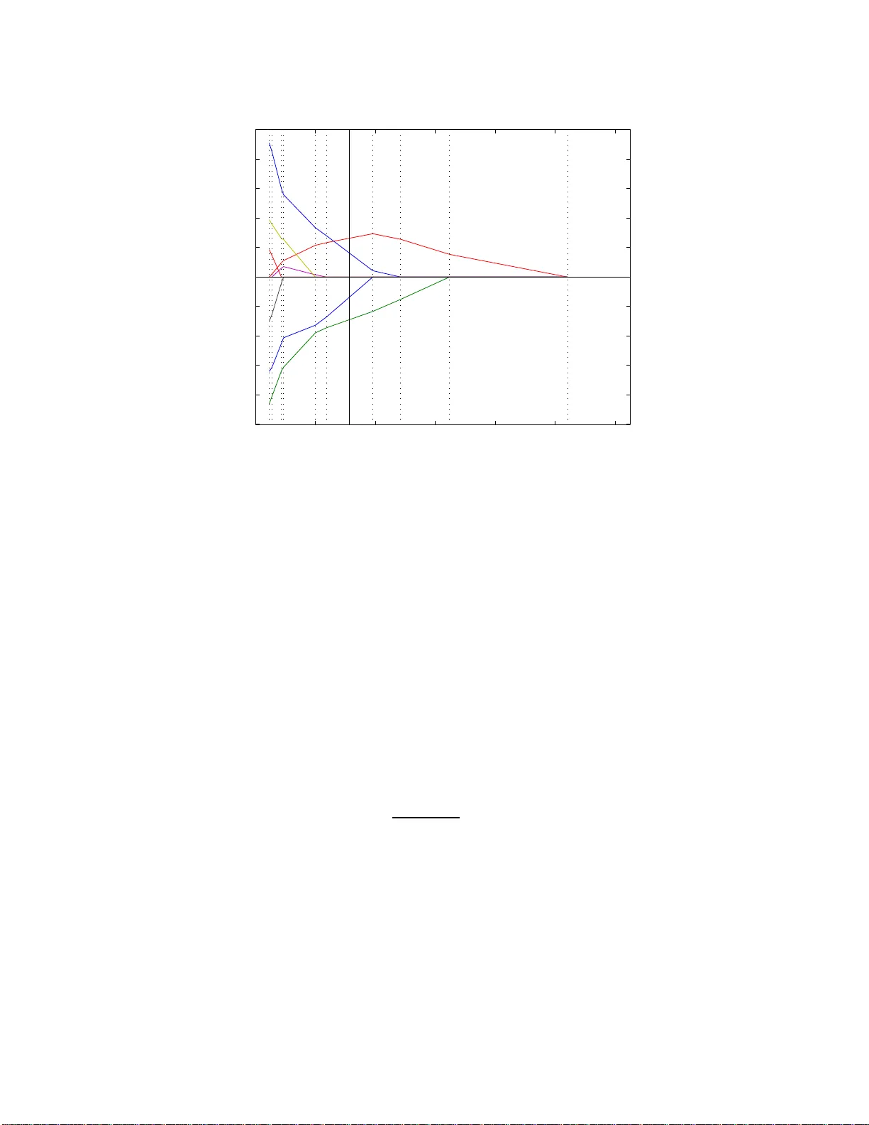
1 A suf ficient condition on monotonic incre ase of the number of nonzero entry in the optimizer of ℓ -1 norm penalized least-square prob lem Junbo Duan, Charles Soussen, Da vi d Brie, J ´ er ˆ ome Idier and Y u-Ping W ang Abstract The ℓ -1 norm b ased optim ization is widely used in sign al pro cessing, especially in recent c ompressed sensing theory . This paper studies the s olution path of the ℓ -1 norm penalized least-square problem, whose constrained form is known as Least Absolute Shrinkage and Selection Operator (LASSO). A solution path is the set of all th e o ptimizers with respect to the ev olu tion of th e hype rparameter (Lagrange multiplier). The study of the solution path is of great significance in viewing and understandin g the profile of the tradeoff between the approx imation and regularization term s. If the so lution path of a giv en p roblem is known, it can help us to find the optimal hyperpar ameter u nder a giv e n criter ion su ch as the A kaike Inform ation Criterion. In th is paper we pr esent a sufficient c ondition on ℓ -1 no rm pe nalized least-squ are problem . Under this sufficient condition , the numbe r of nonzero entries in the optim izer or solution vector increases mo notonica lly whe n the hyperp arameter d ecreases. W e also generalize th e r esult to the often used to tal variation case, where the ℓ -1 norm is taken over the first order deri vativ e of the solution vector . W e prove that the p roposed cond ition has intr insic conn ections with the conditio n g i ven by Do noho et al. [1] and th e positive cone condition by Efron el al [2 ]. Howe ver, the prop osed c ondition does n ot need to assume the sp arsity level o f the signal as r equired by Donoh o et al. ’ s co ndition, an d is easier to verify than Efro n et al. ’ s positive con e con dition wh en b eing used for practical applicatio ns. Keywords J. Duan and Y .-P . W ang are wi th the Department of Bi omedical Engineering and Bi ostatistics, Tu lane Univ ersi ty , New Orleans, USA (e-mail: jduan@tulane.edu; wyp@tulane.edu). C. S oussen and D. Brie are wit h Centre de Recherche en Automatique de Nancy , Nancy Univ ersity , Nancy , France (e-mail: charles.soussen@cran .uhp-nanc y .fr; david.brie@cran .uhp-nanc y .fr). J. Idier is wit h Institut de Recherche en Communication et Cybernetique de Nantes, Nantes, F rance (e-mail: jerome.idier@irccyn.ec-na ntes.fr). Nov ember 16, 2021 DRAFT 2 LASSO, Homotopy , LARS, ℓ -1 nor m, diagonally dominant, comp ressed sensing, k -step solution proper ty , positive cone, and total variation. I . I N T R O D U C T I O N The ℓ -1 norm optimization problem r eceived wildly focus in op timization and signa l proces sing community in the last decade , espe cially in the context of compresse d sensing, becau se of its stable performance in sparse signal restoration [3], [4]. The ℓ -1 norm of a vector u ∈ R n is defined as: k u k 1 = n X i =1 | u i | where u i is the i -th entry of u and | u i | denotes the abso lute value. For a given obs ervation y ∈ R m , a c ommon problem in c ompressed sen sing theory is to estimate the sparse approximation y ≈ Au in a giv en dictionary A ∈ R m × n . The dictionary A c onsists of the eleme ntary sign als we are interested in. Under Ba yesian framew ork, when we assume G aussian distrib u tion on residual r = y − Au and Laplacian distrib ution on u , the above problem can be formulated as [5]: u ∗ ( λ ) = arg min u  E ( u , λ ) = 1 2 k y − Au k 2 + λ k u k 1  (1) The constrained form reads arg min u 1 2 k y − Au k 2 subject to k u k 1 6 τ (LASSO) which is well k nown in the literature as Le ast Abs olute Shrinkage and Selection Operator (LASSO). Becaus e of the eq ui valence o f the two forms as disc ussed in [6], all the results conce rning the pe nalized form ( i.e., (1)) in this p aper can be a pplied straightforward to LASSO . The solution path of o ptimization problem (1) is defined as the set of all the optimizers w .r .t. the ev olution of the hype rparameter: { u ∗ ( λ ) | λ ∈ (0 , ∞ ) } . Fig. 1 sh ows a typical s olution path. Ea ch colored curve corresp onds to a n entry in u . It is significant to fin d the so lution path from bo th the oretical and a pplication point of vie w . If the solution pa th is known, we can have the profile of the tradeoff be tween approximation term k y − Au k 2 and regularization term k u k 1 , which can help us to fi nd the bes t hyperparame ter under g i ven criterion, such as L-curve [7] or Aka ike Information Criterion. For example, each λ corresponds one da ta point ( k u ∗ ( λ ) k 1 , k y − Au ∗ ( λ ) k 2 ) at the 2D plane . All the data points form the Pareto frontier [6]; and we can choos e the data point having the largest curvature as the best tradeoff [7]. Nov ember 16, 2021 DRAFT 3 λ 0 =+ ∞ λ 1 λ k−1 λ k λ K =0 λ u Fig. 1. A typical solution path of problem (1 ). E ach colored curv e corresponds to the ev olution of an entry in u w .r.t. λ . T o find the solution, the Homotopy and LARS algorithm usually start with λ = + ∞ and decrease the v alue step by step. Because it is piece wise linear at the interv al [ λ k , λ k − 1 ] , the solution v alue at λ can be e valuated from solutions at λ k and λ k − 1 by linear interpolation. As a result of the discovery of the piecewise-linear -property of the solution path [8], algorithms lik e Homotopy [9], [10] an d Le ast Angle Regression LARS [2] were developed. The advantage o f piecewise- linear- property is: If we have fin ite solutions { u ∗ ( λ k ) | k = 0 , 1 , . . . , K } , where 0 = λ K < · · · < λ 1 < λ 0 = + ∞ and u ∗ ( λ k )( k = 1 , . . . , K − 1) is the so lution at the boun dary of two pieces, we ca n reconstruct the wh ole solution path for any λ . For any gi ven hy perparameter λ k 6 λ < λ k − 1 , u ∗ ( λ ) c an be ev a luated by linear interpolation: u ∗ ( λ ) = u ∗ ( λ k ) + λ − λ k λ k − 1 − λ k ( u ∗ ( λ k − 1 ) − u ∗ ( λ k )) It is obvious that u ∗ (+ ∞ ) = 0 . As a result, Homotopy and LARS us ually start with λ = + ∞ and decreas e λ step by step, as illustrated in Fig.1. In the iterations, critical value of λ , i.e., λ k and the correspond ing u ∗ ( λ k ) a re calc ulated s tepwisely . It is neces sary to p oint o ut that, during the running of Homotopy algo rithm, an active s et I ( u ) = { i | u i 6 = 0 } is maintaine d at each iteration, which upd ates the nonzero e ntries in u . If u i change s from z ero to non zero, we appen d I with i ; on the contrary , if u i change s from nonz ero to zero, we remove i from I . Nov ember 16, 2021 DRAFT 4 In previous work [1], Do noho et al. sh owed a cond ition on A and y such that the numb er of element in set I , i.e., the cardinality Card [ I ] , inc reases mono tonically when λ decrease s . This is known as k- step solution property , which is more strictly define d in Sec. III-A. So if ( A , y ) satisfies the cond ition yielding k-step so lution property , one only n eeds to append ing the ac tiv e set I with a n ew entry . Therefore, in eac h iteration of Homotopy algorithm, one only nee ds to check the ch ange from zero to nonzero. Computa tion c an thus be reduced. In other words, the Homotopy and LARS 1 yield the same solution path. However , Dono ho et al. ’ s c ondition nee ds the knowledge of original signa l u , i.e., ass uming the spa rsity level, which is usually unknown in prac tical application. Therefore, in this paper we prese nt a sufficient condition in which we do not ass ume the spa rsity level of the signa l. This p aper is organized as follows: In S ec. II, we prese nt the s ufficient condition on mono tonic increase of Card [ I ] when λ de creases . In S ec. III, we d iscuss the con nection betwe en our p roposed co ndition and other existing c onditions. The total v ariation based approxima tion is o ften used in sign al denoising [11], where the the ℓ -1 norm is taken over the fi rst o rder d eri vati ve of the solution vector . Th erefore, in Sec . IV, we extend the su f fi cient c ondition to the total vari ation c ase. W e conclude the paper in Sec. V. I I . S U FFI C I E N T C O N D I T I O N Definition 1. H ∈ R n × n is called (row) diagonally d ominant (DD) if h ii > P j 6 = i | h ij | , ( i = 1 . . . n ) ; called (row) ir reducibly diagonally dominant (IDD) if a t least one row me ets > ins tead of > ; an d H is called (row) strictly diagonally d ominant (SDD) if a ll rows meet > instead of > [12]. Definition 2 (Notations) . 0 k × n ∈ R m × n is null matrix; I n ∈ R n × n is identity; J k × n = [ I k , 0 k × ( n − k ) ] ∈ R k × n ; P is the sq uare pe rmutation matrix of size d epending on the c ontext; and P T is the transpose of P . Lemma 1 (DD preservation property) . If full r a nk sy mmetric matrix H is DD, then ( J k × n P H − 1 P T J T k × n ) − 1 is also DD for any P and for all k = 1 , . . . , n . Pr oof: The Proofs can be found in [13] and [14]. Howev er , we prese nt a more co mprehens ible way of proof in Append ix. Remark 1. Lemma 1 indicates, for an DD m atrix H , if we in ve rt it, extract the pr incipal minor of an y size k × k , then the in ve rse of this princ ipal minor is a lso DD . 1 Here we refer to the original version of LARS. The modified version of LARS which enable the removing of index from activ e set I , is equiv alent to Homotopy . Nov ember 16, 2021 DRAFT 5 Based on Lemma 1, we give o ur main result Theorem 1. F or full rank matrix A ∈ R m × n ( m > n ) , in optimization pr oblem (1), if ( A T A ) − 1 is DD, Card [ I ( u ∗ ( λ ))] increas es monotonica lly when λ decr eases . Pr oof: The dif ferential of E ( u , λ ) is: ∂ E ( u , λ ) = A T ( Au ( λ ) − y ) + λ s ( λ ) here s is the subdifferential of k u k 1 [15], which is defined as: s = ∂ k u k 1 =          s i = 1 , if u i > 0 ; s i = − 1 , if u i < 0 ; s i ∈ [ − 1 , 1] , otherwise. (2) A nec essary condition to the optimization problem (1) is to have 0 ∈ ∂ E ( u , λ ) ; therefore, we have the follo wing system: A T Au ∗ ( λ ) + λ s ∗ ( λ ) = A T y (3) Becaus e u ∗ ( λ ) is piecewise linear [2], for eac h piece [ λ k , λ k − 1 ) , s ∗ ( λ ) is cons tant. Thus we c an fin d a permutation P locally such that the non zero entries and zero entries in u ∗ are re arranged to be u ∗ on ( 6 = 0 ) and u ∗ of f (= 0 ) respe cti vely . In the follo wing, we omit the dependen cy of λ for the sake of brevity . u ∗ = P T   u ∗ on u ∗ of f   (4) s ∗ = P T   s ∗ on s ∗ of f   (5) A T y = P T   y on y of f   (6) By subs tituting (4), (5) and (6) into (3), and left multiplying P , since P T = P − 1 , we hav e P A T AP T   u ∗ on 0   + λ   s ∗ on s ∗ of f   =   y on y of f   (7) which can be rewr itten as:   Ψ Υ Υ T Φ     u ∗ on 0   + λ   s ∗ on s ∗ of f   =   y on y of f   Nov ember 16, 2021 DRAFT 6 or Ψ u ∗ on + λ s ∗ on = y on (8) Υ T u ∗ on + λ s ∗ of f = y of f where Ψ = J k × n P A T AP T J T k × n and k is the length of u ∗ on . Under the condition that ( A T A ) − 1 is DD, from Lemma 1, R = Ψ − 1 is DD. From (8) d u ∗ on dλ = − Rs ∗ on (9) For the i -th e ntry of u ∗ on , i.e., u ∗ on,i ( i = 1 , . . . , k ) du ∗ on,i dλ = − k X j =1 r ij s ∗ on,j = − r ii s ∗ on,i − X j 6 = i r ij s ∗ on,j becaus e s ∗ on,j ∈ [ − 1 , 1] , (1) If u ∗ on,i > 0 , from (2) s ∗ on,i = 1 du ∗ on,i dλ = − r ii − X j 6 = i r ij s ∗ on,j DD 6 − X j 6 = i ( | r ij | + r ij s ∗ on,j ) 6 0 (2) If u ∗ on,i < 0 , from (2) s ∗ on,i = − 1 du ∗ on,i dλ = r ii − X j 6 = i r ij s ∗ on,j DD > X j 6 = i ( | r ij | − r ij s ∗ on,j ) > 0 From above two c ases, we can s ee that | u ∗ on,i ( λ ) | decreas es monoton ically wh en λ increa ses in piece [ λ k , λ k − 1 ) , while | u ∗ of f , i ( λ ) | is equa l to ze ro. Becaus e u ∗ i ( λ ) is co ntinuous for λ > 0 [9], it is straightforward to extend the result to all λ : Whe n λ increases , the absolute value of no nzero entries in u ∗ ( λ ) de crease until to 0, while zero en tries remain 0. Therefore, Card [ I ( u ∗ ( λ ))] decrease s monotonically when λ increase s. In other words, C ard [ I ( u ∗ ( λ ))] increases monotonica lly when λ decrea ses. There exist many matrices satisfying the sufficient c ondition. Obvious examples are the o rthogonal dictionaries like Fourier basis or Ha damard bas is. By Monte Carlo simulation, we a lso stud y the prob- ability of random matrices satisfying the s uf ficient cond ition. For each given configuration ( m, n ) a nd distrib u tion P , 1000 trials A ∈ R m × n are generate d, who se e ntries obey i.i.d. P . P is cho sen as: normal distribution, un iform distribution within interv a l [0 , 1] a nd Bernoulli distrib u tion with parameter p = 0 . 1 , 0 . 5 (the probability for 1 is p , for 0 is 1 − p ). The frequency of ( A T A ) − 1 being DD is shown in Nov ember 16, 2021 DRAFT 7 n m 5 10 15 20 25 30 950 850 750 650 550 450 350 250 150 50 0 10 20 30 40 50 60 70 80 90 100 n m 5 10 15 20 25 30 950 850 750 650 550 450 350 250 150 50 0 10 20 30 40 50 60 70 80 90 100 normal uniform n m 5 10 15 20 25 30 950 850 750 650 550 450 350 250 150 50 0 10 20 30 40 50 60 70 80 90 100 n m 5 10 15 20 25 30 950 850 750 650 550 450 350 250 150 50 0 10 20 30 40 50 60 70 80 90 100 Bernoulli with p = 0 . 1 Bernoulli with p = 0 . 5 Fig. 2. The fr equenc y (in percentage) of ( A T A ) − 1 being DD. Distribution P is chosen as: normal distribution, uniform distribution within interval [0 , 1] and Bernoulli distribution wit h parameter p = 0 . 1 , 0 . 5 . Fig. 2. From the simulation results, we foun d that rand om matrices sa tisfy the su f fi cient condition when m ≫ n . In compress ed sensing (CS) [16], [17 ], ran dom matrix is freque ntly utilized to project a high dimens ion sparse signal into a low dimension sp ace. If the correlation be tween the columns in the random matrix A is low enou gh, an d the original signa l is a lso sparse enou gh, the o riginal s ignal can be recovered from its observation via ℓ -1 op timization or o ther methods. In the n ext section, we show the intrinsic con nection between our result and those deri ved b y Donoho e t al. [1] and and Efron et al. [2] in CS theory . Nov ember 16, 2021 DRAFT 8 I I I . C O N N E C T I O N W I T H O T H E R C O N D I T I O N S A. Connection with Donoho e t al.’ s condition k -step s olution pr o perty: For a gi ven p roblem instan ce ( A , ˜ y ) , where A = [ a 1 , · · · , a n ] ∈ R m × n , ˜ y = A ˜ u , and ˜ u has only k non zero entries. W e say that an algorithm has k -step solution property at this giv e n problem ins tance if it terminates after at mos t k -ste ps with the correct solution ˜ u . In [1], Donoh o gave a condition such that Homotopy a lgorithm h as k -step solution property . Donoho et al.’ s cond ition: For the problem instanc e ( A , ˜ y ) , if the sparsity level k obeys k 6 1 + µ − 1 2 (10) where µ is the mutual coheren ce of A : µ = max i 6 = j | < a i , a j > | then the Homotopy algorithm runs k steps and s tops, deliv e ring the so lution ˜ u . Here < · , · > den otes the inner product. In fact µ is the maximum of absolute value o f off- diagonal en tries of the Gram matrix G = A T A . Throughou t this section, a i is n ormalized for co n venience , i.e., k a i k = 1 . So the diagona l e ntry of G is 1 and µ < 1 . As Homotopy algorithm was proved to be able to find the solution pa th of problem (1) [10], Donoho et al. ’ s con dition can also be viewed as a sufficient condition which yields monotonic increa se of Card [ I ( u ∗ ( λ ))] . Howev er , Donoho et al. ’ s cond ition need to know k , i.e., the sp arsity level of u , whic h is usually unknown in practical applica tions, while in The orem 1, the knowledge of u is not n eeded . Donoho et a l. ’ s co ndition reflects the follo wing fact: lower co rrelated matrix A (sma ller µ ) yields more nonzero entries in u (larger k ) tha t could b e recovered. A na tural dedu ction is for the limit c ase where k = n − 1 , which means u is not sp arse a t all; the up per bou nd of µ is 1 2( n − 1) − 1 = 1 2 n − 3 ( i 6 = j ) , which is coinciden t with Corollary 1 shown below . Theorem 2. Fu ll rank symmetr ic matrix G ∈ R n × n ( n > 2) , if g ii > 0 an d | g ij | g ii 6 1 2 n − 3 , G − 1 is DD. Pr oof: If | g ij | g ii 6 1 2 n − 3 ( j 6 = i ) , P j 6 = i | g ij | g ii 6 n − 1 2 n − 3 < 1 for n > 2 ⇒ G is SDD ⇒ G is positi ve definite and nons ingular [18] ⇒ its in verse H = G − 1 is also positiv e defi nte ⇒ h ii > 0 . From H G = I we hav e: δ ij = X v h iv g vj = X v 6 = j h iv g vj + h ij g j j Nov ember 16, 2021 DRAFT 9 here δ ij is kronecker s ymbol. X j 6 = i | h ij | = X j 6 = i     δ ij − P v 6 = j h iv g vj g j j     = X j 6 = i       − X v 6 = j g vj g j j h iv       6 1 2 n − 3 X j 6 = i X v 6 = j | h iv | = 1 2 n − 3 X j 6 = i X v | h iv | − | h ij | ! = 1 2 n − 3   X j 6 = i X v | h iv | − X j 6 = i | h ij |   = 1 2 n − 3   ( n − 1) X v | h iv | − X j 6 = i | h ij |   = 1 2 n − 3   ( n − 1) X v 6 = i | h iv | + ( n − 1) h ii − X j 6 = i | h ij |   = 1 2 n − 3   ( n − 2) X j 6 = i | h ij | + ( n − 1) h ii   by moving P j 6 = i | h ij | in the right h and side to the left h and side , we have P j 6 = i | h ij | < | h ii | = h ii , so G − 1 = H is DD. Corollary 1. F or s ymmetric matrix G ∈ R n × n with g ii = 1 , | g ij | 6 1 2 n − 3 ( i 6 = j ) , G − 1 is DD. Remark 2. As µ is e qual to the m aximum of absolute v alue of off -diagonal en tries of the Gram matrix G = A T A . µ ≤ 1 2 n − 3 yields ( A T A ) − 1 being DD. The r e for e, Donoho et a l.’ s condition a nd Theorem 1 ar e co nnected via C or ollary 1. B. Connection with Efr on et al.’ s positive cone condition P ositive con e co ndition: For e ach principal minor of B T A T AB , the su m o f e ach row of the in verse matrix of this principal minor is positiv e. Here B is the diagonal matrix whose diagon al entry is ± 1 . In [19 ], Me inshause n p ointed o ut tha t Efron et al. ’ s positiv e c one con dition [2] yields monotonic increase of the abs olute v a lue of the LASSO es timator . In other w ords, the monotonic increa se of the Nov ember 16, 2021 DRAFT 10 number of non zero entry . In fact, from L emma 1 we c an deduce that the p ositi ve cone co ndition is equiv alen t to the condition that ( A T A ) − 1 is SDD. Theorem 3. P ositive co ne co ndition is equivalent to the S DD c ondition on ( A T A ) − 1 . Pr oof: • Positi ve c one c ondition ⇒ SDD condition on ( A T A ) − 1 Each principal minor of B T A T AB can be written as J k × n P B T A T AB P T J T k × n , positi ve cone condition dema nds that for a ny P , B and for a ll k = 1 , . . . , n , the sum of eac h row of its in verse matrix s hould be pos iti ve. For the con figuration where P is the ide ntity matrix an d k = n , the sum o f the i -th row of ( B T A T AB ) − 1 , or B T H B c an be written as P n j =1 b ii b j j h ij = h ii + P j 6 = i b ii b j j h ij ; the positiv e cone c ondition reads h ii + P j 6 = i b ii b j j h ij > 0 . Be cause b ii and b j j could be either +1 or − 1 , proper choic e of b ii and b j j yields h ii > P j 6 = i | h ij | , i.e., H = ( A T A ) − 1 is SDD. • SDD condition on ( A T A ) − 1 ⇒ positiv e co ne co ndition H = ( A T A ) − 1 being SDD yields h ii > P j 6 = i | h ij | > P j 6 = i b ii b j j h ij for any confi guration of B . So the positiv e cone c ondition is true for k = n . From Lemma 1, i.e., the DD (or SDD) p reservation property , the in verse matrix of each p rincipal minor of A T A is also SDD. So the pos iti ve con e condition is true for k < n . Remark 3. Be cause SDD con dition is str onger than DD cond ition, from Theo r e m 1 an d Theorem 3, we find that the po sitive cone con dition ca n b e relaxed in order to hav e the monotonic increase of numb er of nonzero entry . In other words, the positive in pos itive co ne condition can be r elaxed to non negative . In practical applications the positi ve cone c ondition is difficult to test be cause o f the hu ge nu mber o f configurations of both the p rincipal minor and B . On the contrary , the cond ition in T heorem 1 is more practicable. I V . S U FFI C I E N T C O N D I T I O N F O R T OT A L V A R I AT I O N D E N O I S I N G In s ignal proces sing community , the following total variation case is often us ed suc h as in denoising [11]. x ∗ ( λ ) = arg min x  1 2 k y − x k 2 + λ k D x k 1  (11) Nov ember 16, 2021 DRAFT 11 where D could be chosen as the first order deriv ative ma trix of size ( n − 1) × n :         1 − 1 0 · · · 0 0 1 − 1 . . . . . . . . . . . . . . . . . . 0 0 · · · 0 1 − 1         (12) In the follo wing, we prese nt a sufficient con dition, whe re D is no t nece ssarily the first deriv ative matrix. Lemma 2. F or full rank D ∈ R m × n ( m 6 n ) , pr ob lem (11) is equiv alent to the following one u ∗ ( λ ) = arg min u  1 2 k z − Au k 2 + λ k u k 1  (13) where u = D x z = D T ( D D T ) − 1 D y A = D T ( D D T ) − 1 (14) Pr oof: The optimi zation problem (11) i s equiv alent to t h e foll owing constrained op timization problem ( x ∗ ( λ ) , u ∗ ( λ )) = arg min x , u  1 2 k y − x k 2 + λ k u k 1  subject to D x = u (15) The Lagrange function assoc iated with (15) reads L ( x , u , µ ) = 1 2 k y − x k 2 + λ k u k 1 + µ T ( u − D x ) where µ is Lagrange multiplier . The optimality condition reache s ∂ L ∂ x = x − y − D T µ = 0 ∂ L ∂ µ = u − D x = 0 From above two eq uations, w e h av e µ = ( D D T ) − 1 ( u − D y ) x = y + D T ( D D T ) − 1 ( u − D y ) (16) by substituting (16) into (15), (15) rereads u ∗ ( λ ) = arg min u  1 2 k D T ( D D T ) − 1 ( D y − u ) k 2 + λ k u k 1  which is the same as (13) where u , z , a nd A are define d as in (14). So (11) is equ i valent to (13). Nov ember 16, 2021 DRAFT 12 Theorem 4. F or full rank matrix D ∈ R m × n ( m 6 n ) a nd optimization pr oble m (11), if D D T is DD, Card [ I ( x ∗ ( λ ))] increas es monotonica lly when λ decr eases . Pr oof: From Lemma 2, ( A T A ) − 1 = D D T is DD. By applying Theo rem 1 , we g et this the orem straightforwards. It is easy to verify that the first deriv ative matrix (12) s atisfies the co ndition in Theo rem 4. Thu s, the results hold for the optimization problem (11) with total variation cas e. V . C O N C L U S I O N In this paper , we presented a suf fic ient condition und er which the number of nonzero entries in the optimizer of ℓ -1 n orm pen alized lea st-square problem increas es monotonically . Suf fic ient condition for the total vari ation case is a lso prese nted. W e showed tha t the sufficient condition, i.e., the in verse of the Gram matrix of the matrix A is diagona lly do minant, is strongly conne cted with Dono ho et al. ’ s condition and is equiv alent to or more general than Efron et al. ’ s positi ve cone condition. Co mpared with Donoho et al. ’ s condition which yields k -step solution property , our proposed co ndition does not need the knowledge of the original signa l ( i.e., the sparsity le vel), which is us ually u nknown in practical application. Compa red with Efron et al. ’ s positive c one cond ition which need s to tes t a lar g e numb er of configurations in an exhaustive manner , our propo sed c ondition is simpler to verify . A P P E N D I X In order to prove Lemma 1, we introduce the following two Lemmas. Lemma 3. If full rank symmetric matrix H ∈ R n × n is DD, then R = ( J ( n − 1) × n H − 1 J T ( n − 1) × n ) − 1 is also DD. Pr oof: Define: H =   H 11 H 12 H T 12 H 22   G = H − 1 =   G 11 G 12 G T 12 G 22   where H 11 , G 11 are of s ize ( n − 1) × ( n − 1) . The s ub-matrices can be expres sed to H a nd G acco rding Nov ember 16, 2021 DRAFT 13 to H 11 = J ( n − 1) × n H J T ( n − 1) × n H 12 = [ h 1 n , h 2 n · · · h n − 1 ,n ] T H 22 = [ h nn ] (17) G 11 = J ( n − 1) × n GJ T ( n − 1) × n G 12 = [ g 1 n , g 2 n · · · g n − 1 ,n ] T G 22 = [ g nn ] From block matrix in version lemma [18], we know R = G − 1 11 = H 11 − H 12 H − 1 22 H T 12 From above and (17), the entry of R reads r ij = h ij − h in h j n h nn , ( i = 1 . . . n − 1 , j = 1 . . . n − 1) then we have X j 6 = i,n | r ij | = X j 6 = i,n     h ij − h in h j n h nn     6 X j 6 = i,n | h ij | + | h in | h nn X j 6 = i,n | h j n | DD 6 X j 6 = i,n | h ij | + | h in | h nn ( h nn − | h in | ) = X j 6 = i,n | h ij | + | h in | − h 2 in h nn = X j 6 = i | h ij | − h 2 in h nn DD 6 h ii − h 2 in h nn = r ii So R is DD. Lemma 4. If full rank symme tric matrix H ∈ R n × n is DD, then R k = ( J k × n H − 1 J T k × n ) − 1 is a lso DD for all k = 1 , . . . , n − 1 . Nov ember 16, 2021 DRAFT 14 Pr oof: H is full rank symmetric, so R i , ( i = 1 . . . n − 1) is also full rank s ymmetric. By using Lemma 3 recursively: H is DD ⇒ R n − 1 is DD ⇒ R n − 2 is DD ⇒ · · · · · · ⇒ R 1 is DD. Proof of L emma 1 : H is full ra nk symetric DD, so P H P T is a lso full rank s ymetric DD. From Lemma 4, Lemme 1 is straightforward. R E F E R E N C E S [1] D. L. Donoho and Y . Tsaig, “Fast solution of l 1 -norm minimization problems when the solution may be sparse”, IEEE Trans. Inf. Theory , vol. 54, no. 11, pp. 4789–4812, Nov . 2008. [2] B. Efron, T . Hastie, I. Johnstone, and R. T i bshirani, “Least angle regres sion”, Annals Statist. , vol. 32, no. 2, pp. 407–49 9, 2004. [3] J. A. T ropp, “Greed is good: Algorithmic results for sparse approximation”, IEEE T rans. Inf. Theory , vol. 50, no. 10, pp. 2231–2 242, 2004. [4] D. L. Donoho, M. E lad, and V . N. T emlyak ov , “Stable recov ery of sparse ov ercomplete representations in the presence of noise”, IEEE Trans. Inf. Theory , vol. 52, no. 1, pp. 6–18, 2006. [5] M. Nikolov a, “Model distortions in Bayesian MAP reconstruction”, AIMS In verse Problems and Imaging , vol. 1, no. 2, pp. 399–42 2, 2007. [6] E. V an den Berg and M. P . Friedlander , “Probing the pareto frontier for basis pursuit solutions”, T ech. Rep., Univ ersity of British Columbia, Jan. 2008. [7] P . Hansen, “ Analysis of discrete ill-posed problems by means of the L-curve”, SIAM Rev . , vol. 34, pp. 561–580, 1992. [8] R. T ibshirani, “Regression shrinkage and selection via the Lasso”, J. R. Statist. Soc. B , vol. 58, no. 1, pp. 267–288, 1996. [9] M. R. Osborne, B. Presnell, and B. A. T urlach, “ A new approach t o variable selection in least squares problems”, IMA Journal of Numerical Analysis , vol. 20, no. 3, pp. 389–40 3, 2000. [10] D. M. Malioutov , M. Cetin, and A. S. Willsky , “Homotop y continuation for sparse signal representation”, in Proc . I EEE ICASSP , Philadephia, PA , Mar . 2005, vol. V , pp. 733–736. [11] A. Chambolle and P .-L. Lions, “Image r ecov ery via total v ariation minimization and related problems”, Numer . Math. , vol. 76, pp. 167–188, 1997. [12] G. H. Golub and C. F . V an Loan, Matrix computations , The Johns Hopkins University Press, Baltimore, Third edition, 1996. [13] T .-G. Lei, C.-W . W oo, J.-Z. Liu, and F . Z hang, “On t he S chur complement of diagonally dominant matrices”, in SIAM confer ence on applied linear algebra , W il liamsbur g, V A , USA, July 2003. [14] D. Carlson and T . Markham, “Schur complements of diagonally dominant matrices”, Czechoslova k Mathematical J ournal , vol. 29, no. 20, pp. 246–251 , 1979. [15] R. T . R ockafellar , Con vex A nalysis , P rinceton Univ . Press, 1970. [16] D. L. Donoho, “Compressed sensing”, IEEE Trans. Inf. Theory , vol. 52, no. 4, pp. 1289–1306 , 2006. [17] E. J. Cand ` es and M. B. W akin, “ An introduction to compressiv e sampling”, IEEE Signal Processin g Maga zine In Signal Pr ocessing Magazine , pp. 21–30, 2008. [18] D. Bernstein, Matrix Mathematics , Princeton Unive rsity P ress, 2005. [19] N. Meinshausen, “Relaxed Lasso”, Computational Statistics and Data Analysis , vol. 52, no. 1, pp. 374–39 3, Sept. 2007. Nov ember 16, 2021 DRAFT