Robust recovery of multiple subspaces by geometric l_p minimization

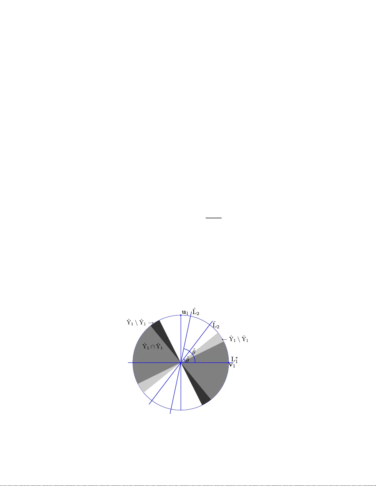
The Annals of Statistics 2011, V ol. 39, No. 5, 2686–27 15 DOI: 10.1214 /11-AOS914 c  Institute of Mathematical Statistics , 2 011 R OBUST RECOVER Y OF MUL TIPLE S UBSP ACES BY GEOMETRIC L P MINIMIZA TION 1 By Gilad Lerman and Teng Zhang University of Minnesota W e assume i.i.d. data sampled from a mixture distribution with K compon ents along fixed d -dimensional linear sub spaces and an addi- tional outlier comp onent. F or p > 0, w e study t h e sim ultaneous reco v- ery of the K fixed subspaces by minimizing the l p -av eraged distances of the sampled data p oints f rom any K subspaces. Under some con- ditions, w e show t hat if 0 < p ≤ 1, then all underlyin g subspaces can b e precisely reco vered by l p minimization with ov erwhelming prob- abilit y . On the other han d , if K > 1 and p > 1, then the underlying subspaces cannot b e reco vered or even nearly recov ered by l p mini- mization. The results of th is pap er partially explain th e successes and failures of the basic approach of l p energy minimization f or modeling data by multiple subspaces. 1. In tro duction. In the last decade, many algorithms ha ve b een dev el- op ed to model data b y m u ltiple subspaces. Suc h h ybr id linea r mo deling (HLM) was motiv ated b y concrete pr oblems in compu ter vision as wel l as b y nonlinear d imensionalit y reduction. HLM is the simp lest geomet ric f rame- w ork for nonlinear dimensionalit y reduction. Nev ertheless, v ery little theory has b een d ev elop ed to ju s tify the p erform an ce of existing metho d s . Here we giv e a rigorous analysis of the r eco ve ry of multiple sub spaces via an energy minimization. One can mo del a data set X with K subspaces obtained b y m inimizing the follo wing energy o ver the sub spaces L 1 , . . . , L K : e l p ( X , L 1 , . . . , L K ) = X x ∈X dist p x , K [ i =1 L i ! , (1) Received Ap ril 2011. 1 Supp orted in part b y NSF Gran ts DMS-09-15064 and DMS-09-56072 . AMS 2000 subje ct classific ations. 62H30, 62G35, 68Q32. Key wor ds and phr ases. Detection, clustering, multiple subspaces, h yb rid linear mod- eling, optimization on the Grassmannian, robustness, geometric probability , high- dimensional data. This is an ele ctronic r eprint of the o riginal ar ticle published by the Institute of Mathematical Statistics in The A nnals of Statistics , 2011, V ol. 3 9 , No. 5, 2 686– 2715 . This reprint differs from the orig inal in pagination and t yp og r aphic detail. 1 2 G. LERMAN AND T. ZHANG where dist( · , · ) denotes the E u clidean distance and p > 0 is a fi xed param- eter. F or simp licit y , we assume th at L 1 , . . . , L K are linear subsp aces of th e same dimension d , and w e refer to them as d -subsp aces (generalizations are discussed in Sections 5.6 and 5.7 ). W e also assume that the data set X con- tains i.i.d. samp les from a mixtur e distribu tion µ with K comp on ents along fixed d -subsp aces and an additional outlier comp onent . The reco very prob- lem asks whether with ov erwh elming probabilit y th e minimization of ( 1 ) reco v ers the u nderlying subsp aces of µ . W e sho w here that when p ≤ 1 the answ er to this problem is p ositive , whereas when p > 1 it is negativ e. Reco very problems are common in statistics, for example, reco v ering a sin- gle su bspace in least squ ares typ e pr oblems or reco v ering m ultiple centers as in K -means. Ho we ve r, our recent setting requires no v el dev elopmen ts. One issue is the strong geometric n ature of our problem, resulting fr om an optimization on a pro d u ct s p ace of Grassmannians. T he other is the diffi- cult y of appr o ximating the p roblem b y con v ex o ptimization (as we clarify in Section 5.1 ). Th us, ev en th ough it is an elemen tary problem in statistical learning, it requ ires the dev elopmen t of tec hn iques wh ic h are currently n ot widely common in statisti cs. 1.1. Backgr ound and r elate d work. Man y algorithms hav e b een devel- op ed for HLM (see, e.g., [ 1 , 5 , 8 – 11 , 13 , 14 , 20 – 26 ]), and they find dive rse applications in several areas, such as motion segmen tation in computer vi- sion, h ybrid linear represen tation of image s, classification of face imag es and temp oral segmen tation of video sequences (see, e.g., [ 14 , 23 , 26 ]). HLM is the simplest n onlinear data modeling and fits within the broader framew orks of modeling dat a b y mixtu r e of manifolds [ 3 ] an d b y Whitney’s stratified space [ 4 ]. The K -subspaces algorithm [ 5 , 10 , 22 ] is the most basic heuristic for HLM, and it suggests an it erativ e pro cedur e attempting to minimize the energy ( 1 ) with p = 2. It generalizes the K -means algorithm, whic h mo dels data b y K cen ters, that is, 0-dimensional affine sub spaces. Numerical exp eriments by Zhang et al. [ 25 ] h a v e shown that the K -subspaces algorithm is in general not rob u st to outliers, wher eas a different metho d aiming to minimize ( 1 ) with p = 1 seems to b e robu st to outliers. There h as b een little in v estigation into p erformance guaran tees of the v arious HLM algorithms. Nevertheless, the accuracy of segmen tation under some sampling assumptions wa s analyzed for t wo sp ectral-t yp e HLM algo- rithms in [ 7 ] and [ 3 ], where [ 3 ] also qu an tified the tolerance to outliers ([ 3 ] considers only the asymptotic case, th ough app lies to mo deling b y multiple manifolds). F or the K -means algorithm (wh ich only a pp lies to 0 -dimensional affine subsp aces), Polla rd has established strong consistency [ 16 ] and a cen- tral limit theorem [ 17 ]. ROBUST RECOVER Y O F MUL TIPLE SUBSP AC ES 3 In [ 12 ], w e analyzed the l p -reco very of the “most significan t” subsp ace among m ultiple sub spaces and outliers with sph erically sym m etric un der- lying distr ibutions. W e assu me here a similar (though wea ke r) u nderlying mo del and rely on some of the estimates already devel op ed there. 1.2. Basic c onventions and notation. W e denote by G( D , d ) the Gr ass- mannian, that is, the manifold of d -subspaces of R D . W e measure distances b et wee n F and G in G( D, d ) b y th e metric dist G (F , G) = v u u t d X i =1 θ 2 i , (2) where { θ i } d i =1 are the principal angles b et w een F and G. W e use this distance since th ere is a simple form ula for the geod esic lines on the Grassmannian equipp ed w ith this distance (see, e.g., [ 12 ], equation 12), whic h is app lied in this pap er. W e d istin gu ish elemen ts in the K -fold pr o duct space G( D , d ) K b y the l ∞ norm, th at is, dist G K ((L 1 , . . . , L K ) , ( ˆ L 1 , . . . , ˆ L K )) = max i =1 ,...,K (dist G (L i , ˆ L i )) . (3) F ollo wing [ 15 ], Section 3.9, w e denote by γ D ,d the “un if orm ” distribution on G( D, d ). W e denote by a ∨ b an d a ∧ b the maxim um and m in im um of a and b , resp ectiv ely . W e designate the supp ort of a d istribution µ by sup p( µ ). By sa ying “with o ve rwh elming probability” or, in short, “w.o.p.,” we mean that the und er lyin g pr obabilit y is at least 1 − C e − N/C , where C is a constan t indep en d en t of N . 1.3. Setting of this p ap er. W e assume an i.i.d. data set X ⊆ R D of size N sampled fr om a mixture distribution repr esen ting a hybrid linear m o del around d istinct d -subspaces, { L ∗ i } K i =1 . W e in fact consider t wo different t yp es of mod els, but b oth of them h a v e the same basic structure. W e assu me K d istributions, µ i , eac h sup p orted on a corresp ond ing an d distinct d -sub s pace, L ∗ i , a noise lev el ε ≥ 0, and an outlier distribution, denoted by µ 0 . F urth ermore, for eac h 1 ≤ i ≤ K we h av e a d istin ct noise distribution ν i,ε with b ounded sup p ort in th e orthogonal complement L ∗ i . W e assume that the p th moments of {k ν i,ε k} K i =1 are smaller than ε p for all 0 < p ≤ 1 ( p < 1 is only n eeded when we consid er l p minimization w ith p < 1). Moreo ver, if ε = 0, then { ν i, 0 } K i =1 are the Dirac δ distrib utions su p p orted on the origin within the corresp onding su b spaces orthogonal to { L ∗ i } K i =1 . W e assume that the underlyin g distributions, { µ i } K i =0 , ha v e b ounded sup- p orts ( or p ossibly su b -Gaussian as explained in S ection 5.3 ). In order to sim- plify our estimates, w e further assu m e that s u pp( µ i ) ⊆ B( 0 , 1) for 0 ≤ i ≤ K . 4 G. LERMAN AND T. ZHANG F rom these pieces we construct the mixture distribution µ ε , µ ε = α 0 µ 0 + K X i =1 α i µ i × ν i,ε , (4) where α 0 ≥ 0, α i > 0 ∀ 1 ≤ i ≤ K and P K i =0 α i = 1. If ε = 0, then for con v e- nience w e r ep lace the notation µ ε b y µ , that is, µ = α 0 µ 0 + K X i =1 α i µ i . (5) Within this basic fr amework, w e analyze t w o differen t mo d els. F or ε ≥ 0 and µ ε as in ( 4 ), we sa y that µ ε is a we akly spheric al ly symmetric H LM dis- tribution with noise leve l ε if the { µ i } K i =1 are generated by rotat ions (in R D ) of a sin gle distribu tion ˆ µ , su c h that ˆ µ ( { 0 } ) < 1 , su pp( ˆ µ ) ⊆ B( 0 , 1) ∩ ˆ L for some d -sub s pace ˆ L ⊂ R D and ˆ µ is spherically s y m metric w ithin ˆ L (i.e., in- v arian t to rotatio ns within ˆ L). Our second mo d el has w eak er assu mptions on the distributions of inliers and a s lightly stronger assumption on the d istribution of outliers. F or ε ≥ 0 and µ ε as in ( 4 ), we say that µ ε is a we ak HLM distribution with noise level ε if µ i ( { 0 } ) < 1 ∀ 1 ≤ i ≤ K , s u pp( µ ε ) ⊆ B( 0 , 1) and fo r some r > 0 the uniform distribution on B( 0 , r ) is absolutely con tin uous w.r.t. the restriction of µ 0 to B( 0 , r ). Our theory u ses t he constan t τ 0 ≡ τ 0 ( d, p, { µ i } K i =1 ). W e dela y its definition to the pro ofs [see ( 11 )], but use it in the formulation of T heorems 1.1 and 1.2 . 1.4. Statistic al pr oblems of this p ap er. W e add ress here tw o statistical problems. The s impler one is implicit in this in tro duction, though cle ar from the pro ofs. It asks w hether the underlyin g sub spaces { L ∗ i } K i =1 can b e reco v- ered when ε = 0 b y minimizing E µ (dist p ( x , S K i =1 L i )) o ver { L i } K i =1 ⊂ G( D , d ) . The main prob lem can b e form ulated using the empirical distr ib ution µ N of i.i.d. sample of s ize N from µ . It asks whether { L ∗ i } K i =1 can b e reco ve red (w.o.p.) b y minimizing E µ N (dist p ( x , S K i =1 L i )), w hic h is equiv alent to min - imizing ( 1 ). In the noisy case, we extend these problems to near reco v ery . When K > 1 and d ≥ 1 , th ese problems are nontrivial and requir e compli- cated geo metric estimates. 1.5. Main the ory. W e fi rst formulate the exact reco v ery of { L ∗ i } K i =1 as the unique global minimizer of the l p energy ( 1 ) when 0 < p ≤ 1. Theorem 1.1. Assume that µ is a we akly spheric al ly symmetric HLM distribution on R D without noise ( ε = 0 ) and with underlying subsp ac es ROBUST RECOVER Y O F MUL TIPLE SUBSP AC ES 5 { L ∗ i } K i =1 ⊆ R D and mixtur e c o e fficients { α i } K i =0 . L et X b e an i.i.d. data set sample d fr om µ . If 0 < p ≤ 1 and α 0 < τ 0 · min i =1 ,...,K α i ·  1 ∧ min 1 ≤ i,j ≤ K dist G (L ∗ i , L ∗ j ) p / 2 p  , (6) then w.o.p. the set { L ∗ 1 , . . . , L ∗ K } is the unique glob al minimizer of the ener- gy ( 1 ) among al l d - subsp ac es in R D . Theorem 1.1 extends to the noisy case b y allo wing n ear-reco very as follo ws (a counterexample for asymptotic exact reco ve ry is sho wn in Section 3.2 ). Theorem 1 .2. Assume that ε > 0 and µ ε is a we akly spheric al ly symmet- ric H LM distribution of noise level ε on R D with K d -subsp ac es { L ∗ i } K i =1 ⊆ R D and mixtur e c o efficients { α i } K i =0 . L et X b e an i.i.d. data sample d fr om µ ε . If 0 < p ≤ 1 and ε < 3 − 1 /p  τ 0 · min i =1 ,...,K α i ·  1 ∧ min 1 ≤ i,j ≤ K dist G (L ∗ i , L ∗ j ) p / 2 p  − α 0  1 /p , (7) then any minimizer of ( 1 ) in G( D , d ) K has a distanc e smal ler than f ≡ f ( ε, K, d, p, { α i } K i =1 ) = 3 1 /p ·  τ 0 min 1 ≤ j ≤ K α j − α 0  − 1 /p · ε (8) fr om one of the p ermutations of (L ∗ 1 , . . . , L ∗ K ) with overwhelming pr ob ability. A t last, w e form ulate the imp ossibility t o reco v er { L ∗ i } K i =1 b y l p minimiza- tion w h en p > 1 (the constan ts δ 0 and κ 0 in our form ulation are estimated in S ection 4.5.5 ). Theorem 1.3. Assume an i.i.d. sample of K d -subsp ac es { L ∗ i } K i =1 ⊂ G( D , d ) fr om the “unif orm” distribution on G( D , d ) , γ D ,d . F or ε ≥ 0 and the sample { L ∗ i } K i =1 , let µ ε b e a we ak HLM distribution with noise leve l ε and let X b e an i.i.d. data set of size N sample d fr om µ ε . If p > 1 and K > 1 , then for almost every { L ∗ i } K i =1 (w.r.t. γ K D ,d ) ther e exist p ositive c onstants δ 0 and κ 0 , indep endent of N , such that for any ε < δ 0 the minimizer of ( 1 ), ˆ L 1 , . . . , ˆ L K , satisfies w.o.p.: dist G K (( ˆ L 1 , . . . , ˆ L K ) , (L ∗ 1 , . . . , L ∗ K )) > κ 0 . (9) The ab o ve theorems h a v e d irect implications f or HLM with sph erically symmetric samp ling along the subsp aces. T heorems 1.1 and 1.2 clarify to some exten t the robustn ess of tw o r ecen t algorithms for HLM, which use the l 1 energy ( 1 ): Median K -Fl ats (MKF) [ 25 ] and Lo cal Best-fit Flats (LBF) [ 27 ]. Theorem 1.3 explains why common HLM s trategies that use the l 2 energy ( 1 ) (e.g. , K - sub spaces) are generally not robust to outliers. 6 G. LERMAN AND T. ZHANG 1.6. Structur e of the p ap er. Theorems 1.1 , 1.2 and 1.3 are prov ed in Sections 2 , 3 and 4 , resp ectiv ely . Section 5 discusses p ossible extensions as w ell as limitations of our theory and suggests some op en d irections. 2. Pro of of Theorem 1.1 . 2.1. Pr eliminaries. W e view th e energy e l p ( X , L 1 , . . . , L K ) as a f u nction defined on G( D , d ) K while b eing conditioned on th e fixed d ata set X . Therefo- re, the m in imizer of e l p ( X , L 1 , . . . , L K ) is an elemen t (L ′ 1 , . . . , L ′ K ) in G( D , d ) K . Since an y p ermutat ion of its K co ord inates in G( D , d ) r esults in another minimizer, we sometimes say that the set { L ′ 1 , . . . , L ′ K } is a minimizer [in- stead of (L ′ 1 , . . . , L ′ K )]. W e denote e l p ( x , L 1 , . . . , L K ) := e l p ( { x } , L 1 , . . . , L K ) and view it as a fu nc- tion on R D × G( D , d ) K . W e denote the s et o f all permutations of (1 , 2 , . . . , K ) by P K . W e designate an op en ball in G( D, d ) by B G (L , r ) as opp osed to the Euclidean op en ball in R D , B( x , r ). W e partition X into th e s u bsets {X i } K i =0 with { N i } K i =0 p oints sampled according to the distributions { µ i } K i =0 . W e define ψ µ 1 ( t ) = µ 1 ( x ∈ R D : − t < | x T v | < t ) , (10) where v is an arbitrarily fi xed un it vecto r in L ∗ 1 [due to the spherical symme- try o f µ 1 within L ∗ 1 , ( 10 ) is indep endent of v ]. W e note that since { µ i } K i =1 are generated by a single distrib ution, ψ µ 1 ( t ) = ψ µ i ( t ) ∀ 2 ≤ i ≤ K . The inv ert- ibilit y of ψ µ 1 is esta blish ed in [ 12 ], App endix A.2 , and an estimate o f ψ µ 1 for a u niform d istribution on a d -dimensional ball app ears in [ 12 ], App en d ix A.1. Theorem 1.1 uses the constan t τ 0 , wh ich w e can n o w d efine as follo w s: τ 0 := (1 − µ 1 ( { 0 } )) · 2 p − 1 · ψ − 1 µ 1 ((1 + (2 K − 1) µ 1 ( { 0 } )) / (2 K )) p ( π √ d ) p . (11) In the sp ecial case where µ 1 is the uniform distribu tion on B(0 ¯ , 1) ∩ L 1 , then the estimate of ψ µ in [ 12 ], Section A.1, implies the follo wing lo w er b ound for τ 0 : τ 0 > 1 2 p +1 · K p · d 3 p/ 2 . Consequent ly , Th eorem 1.1 holds in th is case if τ 0 in ( 6 ) is replaced b y 1 / (2 p +1 · K p · d 3 p/ 2 ). F urther m ore, it follo ws f r om basic scaling arguments that if µ 1 is the uniform distrib ution on B(0 ¯ , r 1 ) ∩ L 1 and supp( µ 0 ) ⊆ B(0 ¯ , r 2 ), where r 1 and r 2 are any p ositive num b ers, th en τ 0 > r p 1 2 p +1 · K p · d 3 p/ 2 · r p 2 . ROBUST RECOVER Y O F MUL TIPLE SUBSP AC ES 7 2.2. Auxiliary lemmata . Th e follo wing lemmata are used through ou t this pro of (Lemma 2.1 is pro ve d in the Ap p end ix and Lemma 2.2 in [ 12 ], Ap- p end ix A.2). Lemma 2.1. Supp ose that L 1 , ˆ L 1 , . . . , ˆ L K ∈ G( D , d ) , p > 0 and µ 1 is a sp he- ric al ly symmetric distribution in B( 0 , 1) ∩ L 1 . If min 1 ≤ j ≤ K dist G (L 1 , ˆ L j ) > ε , then E µ 1 ( e l p ( x , ˆ L 1 , . . . , ˆ L K )) > τ 0 ε p . Lemma 2.2. F or any x ∈ R D and L 1 , L 2 ∈ G( D , d ) , | dist( x , L 1 ) − dist( x , L 2 ) | ≤ k x k dist G (L 1 , L 2 ) . 2.3. Pr o of in exp e ctation. W e v er if y T heorem 1.1 “in expectation,” whe- reas late r sections extend the pro of to hold w.o.p. W e use the follo wing no- tation w.r.t. the fixed d -su b spaces L ∗ 1 , L ∗ 2 , . . . , L ∗ K , ˆ L 1 , ˆ L 2 , . . . , ˆ L K ∈ G( D , d ) : I ( i ) = arg min 1 ≤ j ≤ K dist G (L ∗ i , ˆ L j ) ∀ 1 ≤ i ≤ K (12) and d 0 = min i 1 ,i 2 ,...,i K ∈P K dist G K ((L ∗ i 1 , . . . , L ∗ i K ) , ( ˆ L 1 , . . . , ˆ L K )) . (13) The “exp ected v ersion” of Theorem 1.1 is formulate d and pr o v ed as fol- lo ws. Pr opo s ition 2.1. Supp ose that ˆ L 1 , . . . , ˆ L K ar e arbitr ary sub sp ac es in G( D , d ) , 0 < p ≤ 1 , and I is define d w.r.t. { ˆ L i } K i =1 and the u nderlying sub- sp ac es { L ∗ i } K i =1 . If ( I (1) , . . . , I ( K )) is a p ermutation of (1 , . . . , K ) , then E µ e l p ( x , ˆ L 1 , . . . , ˆ L K ) − E µ e l p ( x , L ∗ 1 , . . . , L ∗ K ) (14) ≥  τ 0 min 1 ≤ j ≤ K α j − α 0  d p 0 . On the other hand, if ( I (1) , . . . , I ( K )) is not a p ermutation of (1 , . . . , K ) , then E µ e l p ( x , ˆ L 1 , . . . , ˆ L K ) − E µ e l p ( x , L ∗ 1 , . . . , L ∗ K ) (15) ≥ τ 0  min 1 ≤ j ≤ K α j  min 1 ≤ i,j ≤ K dist p G (L ∗ i , L ∗ j ) / 2  − α 0 . Pr oof . W e define M = arg max 1 ≤ i ≤ K dist G (L ∗ i , ˆ L I ( i ) ) . 8 G. LERMAN AND T. ZHANG Assume firs t that ( I (1) , . . . , I ( K )) is a p ermutation of (1 , . . . , K ). Using the definition of I , w e ha ve min 1 ≤ j ≤ K dist G (L ∗ M , ˆ L j ) = dist G (L ∗ M , ˆ L I ( M ) ) = dist G K ((L ∗ 1 , . . . , L ∗ K ) , ( ˆ L I (1) , . . . , ˆ L I ( K ) )) (16) = d 0 . Com bining ( 16 ) with Lemma 2.1 , we obtain that E µ M e l p ( x , ˆ L 1 , . . . , ˆ L K ) − E µ M e l p ( x , L ∗ 1 , . . . , L ∗ K ) (17) = E µ M e l p ( x , ˆ L 1 , . . . , ˆ L K ) > τ 0 d p 0 . F or an y x ∈ X 0 , le t m ( x ) = arg min 1 ≤ i ≤ K dist( x , L ∗ i ), ˆ m ( x ) = arg min 1 ≤ i ≤ K dist( x , ˆ L i ) and note that e l p ( x , ˆ L 1 , . . . , ˆ L K ) − e l p ( x , L ∗ 1 , . . . , L ∗ K ) = dist( x , ˆ L ˆ m ( x ) ) p − dist( x , L ∗ m ( x ) ) p ≥ dist( x , ˆ L ˆ m ( x ) ) p − dist( x , L ∗ I − 1 ( ˆ m ( x )) ) p (18) ≥ −k x k p dist G ( ˆ L ˆ m ( x ) , L ∗ I − 1 ( ˆ m ( x )) ) p ≥ −k x k p d p 0 ≥ − d p 0 , where th e seco nd inequalit y in ( 18 ) uses Lemma 2.2 . Therefore, E µ 0 e l p ( x , ˆ L 1 , . . . , ˆ L K ) − E µ 0 e l p ( x , L ∗ 1 , . . . , L ∗ K ) > − d p 0 . (19) A t last, we observe that E µ e l p ( x , ˆ L 1 , . . . , ˆ L K ) − E µ e l p ( x , L ∗ 1 , . . . , L ∗ K ) ≥ α M ( E µ M e l p ( x , ˆ L 1 , . . . , ˆ L K ) − E µ M e l p ( x , L ∗ 1 , . . . , L ∗ K )) (20) + α 0 ( E µ 0 e l p ( x , ˆ L 1 , . . . , ˆ L K ) − E µ 0 e l p ( x , L ∗ 1 , . . . , L ∗ K )) . The p rop osition in this case thus follo ws from ( 17 ), ( 19 ) and ( 20 ). Next, we assume that I (1) , . . . , I ( K ) is not a p ermuta tion of 1 , 2 , . . . , K . In this case, there exist 1 ≤ n 1 , n 2 ≤ K suc h that I ( n 1 ) = I ( n 2 ) and, conse- quen tly , 2 min 1 ≤ j ≤ K dist G (L ∗ M , ˆ L j ) = 2 dist G (L ∗ M , ˆ L I ( M ) ) ≥ dist G (L ∗ n 1 , ˆ L I ( n 1 ) ) + dist G (L ∗ n 2 , ˆ L I ( n 2 ) ) (21) ≥ dist G (L ∗ n 1 , L ∗ n 2 ) ≥ min 1 ≤ i,j ≤ K dist G (L ∗ i , L ∗ j ) . ROBUST RECOVER Y O F MUL TIPLE SUBSP AC ES 9 Com bining ( 21 ) and Lemma 2.1 [applied with ε = min 1 ≤ i,j ≤ K dist G (L ∗ i , L ∗ j ) / 2], we obtain that E µ M e l p ( x , ˆ L 1 , . . . , ˆ L K ) − E µ M e l p ( x , L ∗ 1 , . . . , L ∗ K ) (22) > τ 0  min 1 ≤ i,j ≤ K dist G (L ∗ i , L ∗ j ) / 2  p . Finally , since the su p p ort of µ 0 is cont ained in B( 0 , 1), we note that E µ 0 e l p ( x , ˆ L 1 , . . . , ˆ L K ) − E µ 0 e l p ( x , L ∗ 1 , . . . , L ∗ K ) ≥ − 1 . (23) The p rop osition is thus concluded from ( 20 ), ( 22 ) and ( 23 ).  2.4. Pr o of in a lo c al b al l by c alculus on the Gr assmannian. W e cannot directly extend ( 14 ) to an estimate w.o .p., since its lo w er bou n d is a multipli- cation of d p 0 , whic h approac hes zero as the set { L i } K i =1 approac hes { L ∗ i } K i =1 . W e will need to exclude a ball in G( D , d ) K around { L ∗ i } K i =1 b efore suc h an extension. W e thus p ro v e here that { L ∗ i } K i =1 is a unique global minimizer w.o.p. in a lo cal ball. In Section 2.5 we extend Prop osition 2.1 to an estimate w.o.p. outside this ball and conclude th e th eorem. W e show that there exists a sufficien tly small num b er γ 1 suc h that { L ∗ i } K i =1 is the un ique global minimizer w.o.p. of e l p in B G ((L ∗ i 1 , . . . , L ∗ i K ) , γ 1 ). S ince e l p is p erm utation inv arian t, it is also the uniqu e global minimizer in [ i 1 ,i 2 ,...,i K ∈P K B G ((L ∗ i 1 , . . . , L ∗ i K ) , γ 1 ) . In ord er to simplify notation in this part of the pro of, w e will ad op t WLOG the con v ent ion th at th e RHS of ( 3 ) o ccur s at i = 1, that is, dist G (L ∗ 1 , ˆ L 1 ) = max i =1 ,...,K (dist G (L ∗ i , ˆ L i )) . (24) F ollo wing this con ve ntio n and the fact that e l p ( P K i =2 X i , L ∗ 1 , . . . , L ∗ K ) = 0, it is enough to pr o v e that (L ∗ 1 , . . . , L ∗ K ) is the u nique global minimizer w.o.p. of e l p ( X 0 ∪ X 1 , L 1 , . . . , L K ) in B G ((L ∗ 1 , . . . , L ∗ K ) , γ 1 ), f or su fficien tly small γ 1 . Let t 0 := dist G (L ∗ 1 , ˆ L 1 ). F or eac h 1 ≤ i ≤ K , we parametrize according to arc length the geo desic lines from L ∗ i to ˆ L i b y functions L i ( t ), 1 ≤ i ≤ K , on the in terv al [0 , t 0 ] suc h that L i (0) = L ∗ i and L i ( t 0 ) = ˆ L i . (25) W e will pro v e that for sufficien tly small γ 1 > 0, d d t p ( e l p ( X 0 ∪ X 1 , L 1 ( t ) , . . . , L K ( t ))) > 0 for all 0 ≤ t ≤ γ 1 w.o.p. (26) This will clearly imply our desired result. Our p ro of of ( 26 ) is based on the follo wing estimate: d d t p ( e l p ( x , L 1 ( t ) , . . . , L K ( t )))     t =0 ≥ −k x k . (27) 10 G. LERMAN AND T. ZHANG In order to establish ( 27 ), w e denote j = arg min 1 ≤ i ≤ K dist( x , L ∗ i ) and app ly Lemma 2.2 to obtain that d d t p ( e l p ( x , L 1 ( t ) , . . . , L K ( t )))     t =0 = lim t → 0 dist( x , L j ( t )) p − dist( x , L j (0)) p t p (28) ≥ −k x k lim t → 0 dist G (L j ( t ) , L j (0)) p t p . W e also n ote that for all 0 ≤ t ≤ t 0 , dist G (L j ( t ) , L j (0)) p t p ≤ dist G (L 1 ( t ) , L 1 (0)) p t p = 1 . (29) Indeed, if t = t 0 , the inequalit y in ( 29 ) follo ws from ( 24 ) and the equ alit y follo w s f rom ( 25 ). Moreo v er, b oth of them extend to 0 ≤ t < t 0 b y the un- derlying p rop erty of arc length parametrization. Equation ( 27 ) thus f ollo w s from ( 28 ) and ( 29 ). Com bining ( 27 ) with Ho effding’s inequalit y , we obtain that d d t p ( e l p ( X 0 , L 1 ( t ) , . . . , L K ( t )))     t =0 ≥ − X x ∈X 0 k x k ≥ − α 0 N w.o.p. (30 ) W e similarly derive an equation analogous to ( 30 ) w hen r eplacing X 0 with X 1 b y applying some argum en ts of the pr o of of Lemma 2.1 and Ho- effding’s inequalit y as follo ws: d d t p ( e l p ( X 1 , L 1 ( t ) , . . . , L K ( t )))     t =0 = d d t ( e l 1 ( X 1 , L 1 ( t )))     t =0 (31) ≥ τ 0 α 1 N w.o.p. A t last, com binin g ( 30 ), ( 31 ) and ( 6 ), we obtain th at there exists γ ′ 1 ≡ γ ′ 1 ( D , d, K, p, α 0 , α 1 ) suc h that w.o.p. d d t p ( e l p ( X 0 ∪ X 1 , L 1 ( t ) , . . . , L K ( t )))     t =0 ≥ ( τ 0 α 1 − α 0 ) N > γ ′ 1 N . Using the arguments of the pr o of of [ 12 ], equation (35), we conclude that there exists a c onstant γ 1 ≡ γ 1 ( D , d, K, p, α 0 , α 1 , min 2 ≤ i ≤ K dist(L ∗ 1 , L ∗ i ) , µ 0 , µ 1 ) > 0 suc h that ( 26 ) holds. 2.5. Conclusion of The or em 1.1 . In order to conclude the theorem, it is enough to pro v e that { L ∗ 1 , . . . , L ∗ K } is the unique global minimizer w.o.p. of e l p ( X 0 ∪ X 1 , L 1 , . . . , L K ) in the set GP( D , d, γ 1 ) := G( D , d ) K / [ i 1 ,i 2 ,...,i K ∈P K B G ((L ∗ i 1 , . . . , L ∗ i K ) , γ 1 ) . (32) ROBUST RECOVER Y O F MUL TIPLE SUBSP AC ES 11 Com bining Pr op osition 2.1 , the fact that d 0 > γ 1 [whic h follo ws from the definition of d 0 in ( 13 )], Ho effding’s inequalit y and ( 6 ), w e obtain that there exists γ 2 ≡ γ 2 ( D , d, K, p, α 0 , min 1 ≤ i ≤ K α i , min 1 ≤ i 6 = j ≤ K dist(L ∗ i , L ∗ j ) , µ 0 , µ 1 ) > 0 suc h that for an y fixed ( ˆ L 1 , . . . , ˆ L K ) ∈ GP( D , d, γ 1 ), e l p ( X , ˆ L 1 , . . . , ˆ L K ) − e l p ( X , L ∗ 1 , . . . , L ∗ K ) > γ 2 N w.o.p. (33) F ollo wing the pro of of [ 12 ], Th eorem 1.1 [i.e., c o ve ring GP( D , d, γ 1 ) by balls], w e easily extend ( 33 ) w.o.p. f or all K subspaces in the set GP( D , d, γ 1 ) (instead of fixed ones) and th us conclude the theorem. 3. Pro of of Theorem 1.2 and a coun terexample to asymptotic r eco very . 3.1. Pr o of of The or em 1.2 . F ollo wing the argumen t of [ 12 ], Sectio n 3.5. 1, w e redu ce the v erifi cation of Theorem 1.2 to pro ving that there exists a con- stan t γ 3 > 0 suc h that if for all p ermuta tions i 1 , . . . , i K ∈ P K , ˆ L 1 , . . . , ˆ L K ∈ G( D , d ) satisfy that dist G K ((L ∗ i 1 , . . . , L ∗ i K ), ( ˆ L 1 , . . . , ˆ L K )) > f , then E µ ( e l p ( x , ˆ L 1 , . . . , ˆ L K )) > E µ ( e l p ( x , L ∗ 1 , . . . , L ∗ K )) + γ 3 + 2 ε p . (34) In view of Prop osition 2.1 , in order to conclude ( 34 ), it is s u fficien t to v erify that  τ 0 min 1 ≤ j ≤ K α j − α 0  f p > γ 3 + 2 ε p (35) and τ 0 min 1 ≤ j ≤ K α j min 1 ≤ i,j ≤ K dist p G (L ∗ i , L ∗ j ) / 2 p − α 0 > γ 3 + 2 ε p . (36) Setting γ 3 = ε p / 2, ( 35 ) follo ws from ( 8 ) and ( 36 ) follo ws from ( 7 ). 3.1.1. R emark on the size of ε . If ε > π √ d 3 − 1 /p  τ 0 min 1 ≤ j ≤ K α j − α 0  1 /p / 2 , (37) then f > π √ d/ 2, so that there is no restriction on the minimizer of ( 1 ) in G( D , d ) K . It thus mak es sense to fu r ther restrict ε to b e at least lo w er than the righ t-hand sid e of ( 37 ). 3.2. A c ounter example to exact asymptotic r e c overy with noise. One ma y ask if it is p ossib le in the noisy setting ( ε > 0 ) to reco ver the underlying sub- spaces as the num b er of sampled p oin ts, N , app roac hes infin it y . T he answ er to this question is p ositive wh en K = 1 (see, e.g., [ 2 ], Section 11.6, [ 18 ]) or d = 0 (see [ 17 ]). Ho wev er, it is often n egativ e when d > 1 and K > 1, as w e demonstrate in Figure 1 (a) and explain b elo w. In this example, D = 2, K = 2, d = 1 , α 0 = 0 and the t wo underlyin g distributions µ 1 and µ 2 (corre- sp ond ing to the t wo un derlying lines L ∗ 1 and L ∗ 2 ) are un iformly distribu ted 12 G. LERMAN AND T. ZHANG (a) (b) Fig. 1. A c ounter example showing that exact r e c overy with noise is i mp ossible even asymptotic al ly. (a) Gr ay r e gions of unif orm distributions ar ound the two underlying lines. (b) The gr ay r e gion is the interse ction of Y 1 with the uniform distribution r e gion ar ound L ∗ 1 . The b est l p line in Y 1 is ˜ L 1 . in the t w o gra y regio ns demonstr ated in this figur e (the r egion aroun d L ∗ 1 is a r ectangle and the region around L ∗ 2 is a union of t w o disjoint rectangles). In order to verify that th is is indeed a coun terexample, we use a V oronoi- t yp e r egion, which allo ws us to reduce app ro ximation by m ultiple sub spaces to a ppr o ximation b y a single subspace on it. Suc h regio ns { Y i } K i =1 , wh ic h are frequent ly used in Section 4 , are obtained by a V oronoi diagram (restricted to the unit ball) of giv en d -subs p aces { L i } K i =1 ⊆ G( D , d ) as follo ws: Y i (L 1 , . . . , L K ) (38) = { x ∈ B( 0 , 1) : dist ( x , L i ) < d ist( x , L j ) ∀ j : 1 ≤ j 6 = i ≤ K } . These regions are useful to us due to the follo wing elemen tary p rop osition, whose trivial pro of is describ ed in the App endix . Pr opo s ition 3.1. If L ′ 1 , . . . , L ′ K ∈ G( D , d ) , ν is a pr ob ability me asur e on R D and (L ′ 1 , . . . , L ′ K ) = arg min (L 1 ,..., L K ) ∈ G( D,d ) K E ν ( e l p ( x , L 1 , . . . , L K )) , then L ′ 1 = arg min L 1 ∈ G( D,d ) E ν ( e l p ( x , L 1 ) I ( x ∈ Y 1 (L ′ 1 , L ′ 2 , . . . , L ′ K ))) . (39) W e claim that for any fixed p > 0, the distance b etw een { L ∗ 1 , L ∗ 2 } and th e global minimizer of ( 1 ) in the setting of this example is b ounded from b elo w w.o.p. by a p ositiv e constan t indep endent of the sample size, N , for suffi- cien tly large N . Equiv alen tly , w e claim that the distance b etw een { L ∗ 1 , L ∗ 2 } and the g lobal minimizer of E µ ε (dist p ( x , S K i =1 L i )) is p ositiv e, w h ere µ ε is the underlying mixture distribution for this example. In view of P r op osition 3.1 , ROBUST RECOVER Y O F MUL TIPLE SUBSP AC ES 13 w e only need to s h o w a p ositiv e distance b et w een L ∗ 1 and the min imizer of E µ ε ( e l p ( x , L) I ( x ∈ Y 1 )), where Y 1 = Y 1 (L ∗ 1 , L ∗ 2 ). W e r efer to this minimizer as the b est l p line for Y 1 and denote it by ˜ L 1 (while arbitrarily fixing p ). W e note that for an y p > 0, th e integral of l p distances of p oin ts in the p art of Y 1 ab o ve L ∗ 1 from the line L ∗ 1 is sm aller than the similar in tegral in the b ottom part. T herefore, ˜ L 1 is different than L ∗ 1 and the r esp ectiv e orien tation of the t w o lines is demonstrated in Figur e 1 (b). The claim is thus concluded. 4. Pro of of Theorem 1.3 . 4.1. Pr eliminaries. 4.1.1. Notation. W e designate the pro jection from R D on to its sub s pace L b y P L and th e corresp onding orthogo nal pr o jec tion b y P ⊥ L . W e defi ne D L , x ,p = P L ( x ) P ⊥ L ( x ) T dist( x , L) ( p − 2) . (40) W e frequ en tly use the V oronoi-t yp e regions { Y i } K i =1 defined in ( 38 ) with resp ect to the su b spaces { L ∗ i } K i =1 and p ossibly tw o additional arbitrary sub- spaces denoted by ˆ L 2 ∈ G( D , d ) and ˜ L 2 ∈ G( D , d ) . W e will use the follo wing short n otation for 1 ≤ i ≤ K : ˆ Y i = Y i (L ∗ 1 , ˆ L 2 , L ∗ 3 , . . . , L ∗ K ) , ˜ Y i = Y i (L ∗ 1 , ˜ L 2 , L ∗ 3 , . . . , L ∗ K ) (41) and Y i = Y i (L ∗ 1 , L ∗ 2 , L ∗ 3 , . . . , L ∗ K ) . (42) W e denote by ¯ Y i the closure of Y i , that is, ¯ Y i = { x ∈ B( 0 , 1) : d ist( x , L ∗ i ) ≤ d ist( x , L ∗ j ) ∀ j : 1 ≤ j 6 = i ≤ K } . (43) Similarly , the closure of ˆ Y i is den oted by ¯ ˆ Y i . Let L k denote the k th-dimensional L eb esgue m easure. W e den ote d ∗ = d ∧ ( D − d ) and let θ d ∗ (L ∗ i , L ∗ j ) b e the d ∗ th largest prin cipal angle b et we en the d -sub spaces L ∗ i and L ∗ j . Our analysis u ses the distribu tion µ ≡ α 0 µ 0 + P K i =1 α i µ i , ev en though the u n derlying distribution of our mo del is µ ε . F or L , L ∗ ∈ G( D , d ), w e define the “orthogonal su btraction” ⊖ as follo ws: L ∗ ⊖ L = L ∗ ∩ (L ∩ L ∗ ) ⊥ . 4.1.2. Auxiliary lemmata. Using th e notation ab ov e, w e formulate tw o lemmata, whic h will b e used throughout this proof. The pro of of Lemma 4.1 is iden tical to that of [ 12 ], Prop osition 2.2 (while replacing sums by exp ec- tations), w hereas Lemma 4.2 is prov ed in the App endix . Lemma 4.1. F or any L ∗ ∈ G( D , d ) and distribution µ , a ne c essary c on- dition for L ∗ to b e a lo c al minimum of E µ ( l p ( x , L)) is E µ ( D L ∗ , x ,p ) = 0 . (44) 14 G. LERMAN AND T. ZHANG The next lemma quantifies the sen sitivit y of the region Y j , where 1 ≤ j ≤ K , to p erturbations in th e sub space L i , wh ere 1 ≤ i 6 = j ≤ K . WLOG w e formulate it with j = 1 and i = 2 [note that we use the short notation of ( 41 )]. Lemma 4.2. If ˆ L 2 , L ∗ 1 , L ∗ 2 , . . . , L ∗ K ar e sub sp ac es in G( D , d ) such that ˆ L 2 6 = L ∗ 2 , min j 6 =2 ( θ d ∗ ( ˆ L 2 , L ∗ j )) > 0 , min 1 ≤ i 6 = j ≤ K ( θ d ∗ (L ∗ i , L ∗ j )) > 0 (4 5) and θ d ∗ ( ˆ L 2 , L ∗ 1 ) ∨ θ d ∗ (L ∗ 2 , L ∗ 1 ) ≤ min 3 ≤ i ≤ K θ d ∗ (L ∗ i , L ∗ 1 ) , (46) then L D (( ˆ Y 1 \ Y 1 ) ∪ (Y 1 \ ˆ Y 1 )) > 0 . (47) 4.2. A sp e cial c ase. The pr o of of Theorem 1.3 is rather inv olv ed. In order to deve lop a simple intuition, w e pr o vide an element ary pro of of the very sp ecial case where d = 1 , p = 2 a nd K = 2. F or simplicit y we also assu me that D = 2, th ou gh our argument easily ext ends to D > 2. Fig ure 2 sh ows the t wo underlying lines L ∗ 1 and L ∗ 2 and th eir corresp onding regions Y 1 and Y 2 . W e note that the b est l 2 lines [in G( D, 1)] for µ 0 restricted to Y 1 and Y 2 are the cen tral axes of those regions. Since α 0 > 0, the b est l 2 lines [in G( D, 1)] for µ restricted to Y 1 and Y 2 (denoted by ˜ L 1 and ˜ L 2 , resp.) must reside b et we en the b est l 2 lines for µ 0 restricted to Y 1 and Y 2 and L ∗ 1 and L ∗ 2 , resp ectiv ely . In particular, they are different from L ∗ 1 and L ∗ 2 as d emonstrated in the Fig. 2. Il lustr ative pr o of of The or em 1.3 in the sp e cial c ase wher e p = 2 , d = 1 , D = 2 and K = 2 . ROBUST RECOVER Y O F MUL TIPLE SUBSP AC ES 15 figure. Therefore, E µ ( e l 2 ( x , L ∗ 1 , L ∗ 2 )) > E µ ( e l 2 ( x , ˜ L 1 , ˜ L 2 )). Th is implies that w.o.p. e l 2 ( X , L ∗ 1 , L ∗ 2 ) > e l 2 ( X , ˜ L 1 , ˜ L 2 ). 4.3. R e duction of the statement of The or em 1.3 to simpler f ormulations. 4.3.1. R e duction I : U sing the V or onoi-typ e r e g ions { Y i } K i =1 . W e will sh o w here that the follo wing equation implies Theorem 1.3 : γ K D ,d ( { L ∗ i } K i =1 ⊂ G( D , d ) : E µ 0 ( I ( x ∈ Y j ) D L ∗ j , x ,p ) = 0 ∀ 1 ≤ j ≤ K ) = 0 . (48) First, we apply th e argumen t of [ 12 ], Section 3.6.1 (whic h requir es the assumption sp ecified in Section 1.3 that the fi rst momen ts of {k ν i,ε k} K i =1 are smaller than ε ) to obtain that Th eorem 1.3 follo ws by th e equatio n γ K D ,d  { L ∗ i } K i =1 ⊂ G( D , d ) : (L ∗ 1 , . . . , L ∗ K ) (49) = arg min (L 1 ,..., L K ) E µ ( e l p ( x , L 1 , . . . , L K ))  = 0 . Next, applying Prop osition 3.1 , w e conclude that ( 49 ) is a direct conse- quence of the equation: γ K D ,d  { L ∗ i } K i =1 ⊂ G( D , d ) : L ∗ j = arg min L ∈ G( D,d ) E µ ( e l p ( x , L) I ( x ∈ Y j )) (50) ∀ 1 ≤ j ≤ K  = 0 . F urtherm ore, applying Lemm a 4.1 with µ = µ | Y j , we obtain th at ( 50 ) follo ws b y the equation γ K D ,d ( { L ∗ i } K i =1 ⊂ G( D , d ) : E µ ( I ( x ∈ Y j ) D L ∗ j , x ,p ) = 0 ∀ 1 ≤ j ≤ K ) = 0 . (51) A t last w e conclude th e desired r eduction by noting that ( 51 ) and ( 48 ) are equiv alen t [ind eed, the only relev ant comp onents of the d istribution µ in ( 51 ) are µ 0 and µ j and th e corresp onding exp ectatio n according to µ j is zero]. 4.3.2. R e duction I I : F r om K subsp ac es to a single subsp ac e. W e r ed u- ce ( 48 ) so that it s und erlying condition in volv es a single subsp ace as follo ws: γ D ,d  L ∗ 2 ∈ G( D , d ) : min 1 ≤ i 6 = j ≤ K θ d ∗ (L ∗ i , L ∗ j ) > 0 , (52) arg min 2 ≤ i ≤ K θ d ∗ (L ∗ 1 , L ∗ i ) = 2 , E µ 0 ( I ( x ∈ Y 1 ) D L ∗ 1 , x ,p ) = 0  = 0 . W e remark that some of the underlying technical conditions of ( 52 ) app ear in ( 45 ) and ( 46 ) and will b e better understo o d later when app lyin g Lemma 4.2 . W e v erify this r eduction as follo w s. WLOG ( 52 ) can b e form ulated by re- placing L ∗ 2 with L ∗ k , for some 3 ≤ k ≤ K , wh ile letting arg min 2 ≤ i ≤ K θ d ∗ (L ∗ 1 , 16 G. LERMAN AND T. ZHANG L ∗ i ) = k . C ombining this observ ation with elemen tary pr op erties of distribu - tions, we hav e that γ K D ,d ( { L ∗ i } K i =1 ⊂ G( D , d ) : E µ 0 ( I ( x ∈ Y j ) D L ∗ j , x ,p ) = 0 ∀ 1 ≤ j ≤ K ) ≤ K X k =2 Z G( D,d ) K − 1 γ D ,d  L ∗ k : min 1 ≤ i 6 = j ≤ K θ d ∗ (L ∗ i , L ∗ j ) > 0 , arg min 2 ≤ i ≤ K θ d ∗ (L ∗ 1 , L ∗ i ) = k , E µ 0 ( I ( x ∈ Y 1 ) D L ∗ 1 , x ,p ) = 0 |{ L ∗ i } 1 ≤ i 6 = k ≤ K  d( γ K − 1 D ,d ( { L ∗ i } 1 ≤ i 6 = k ≤ K )) + γ K D ,d  { L ∗ i } K i =1 ⊂ G( D , d ) : min 1 ≤ i,j ≤ K θ d ∗ (L ∗ i , L ∗ j ) = 0  = 0 . 4.4. Concluding the c ases d = 1 and d = D − 1 . W e assume fir st that d = 1 . W e conclud e the t heorem in this case b y pro ving ( 52 ) and then ext end the analysis to the case d = D − 1. 4.4.1. R e duction of ( 52 ) using additional c ondition on the Gr assmannian. W e fix v 1 to b e one of the tw o un it v ectors sp an n ing L ∗ 1 and denote by u 1 the unit v ector sp anning (L ∗ 1 + L ∗ 2 ) ∩ L ∗⊥ 1 ha ving orient ation such that for an y p oin t x ∈ L ∗ 2 : ( x T u 1 )( x T v 1 ) ≥ 0. W e will prov e th at ( 52 ) follo ws f rom the follo wing equ ation, whic h introd uces a restriction on the Grassmann ian: γ D ,d  L ∗ 2 ∈ G( D , d ) : min 1 ≤ i 6 = j ≤ K θ d ∗ (L ∗ i , L ∗ j ) > 0 , arg min 2 ≤ i ≤ K θ d ∗ (L ∗ 1 , L ∗ i ) = 2 , (53) E µ 0 ( I ( x ∈ Y 1 ) D L ∗ 1 , x ,p ) = 0 | (L ∗ 1 + L ∗ 2 ) ∩ L ∗⊥ 1 = Sp( u 1 )  = 0 . W e defin e the follo wing sub s et of the sphere S D − 1 : Ω 0 = { x ∈ S D − 1 : x ⊥ v } , and a distribution ω on Ω 0 suc h that for any A ⊆ Ω 0 : ω (A) = γ D ,d (L ∗ 2 ∈ G( D , d ) : (L ∗ 1 + L ∗ 2 ) ∩ L ∗⊥ 1 ∈ Sp(A)). Using this notation, ( 53 ) implies ( 52 ) as follo w s: γ D ,d  L ∗ 2 ∈ G( D , d ) : min 1 ≤ i 6 = j ≤ K θ d ∗ (L ∗ i , L ∗ j ) > 0 , arg m in 2 ≤ i ≤ K θ d ∗ (L ∗ 1 , L ∗ i ) = 2 , E µ 0 ( I ( x ∈ Y 1 ) D L ∗ 1 , x ,p ) = 0  = Z Ω 0 γ D ,d  L ∗ 2 : min 1 ≤ i 6 = j ≤ K θ d ∗ (L ∗ i , L ∗ j ) > 0 , arg min 2 ≤ i ≤ K θ d ∗ (L ∗ 1 , L ∗ i ) = 2 , E µ 0 ( I ( x ∈ Y 1 ) D L ∗ 1 , x ,p ) = 0 | (L ∗ 1 + L ∗ 2 ) ∩ L ∗⊥ 1 = Sp( u 1 )  d( ω ( u 1 )) = 0 . ROBUST RECOVER Y O F MUL TIPLE SUBSP AC ES 17 4.4.2. Pr o of of ( 53 ). W e will sho w that at most one element satisfies the underlying condition of ( 53 ) (i.e., it is a member of th e set for which γ D ,d is ev aluated). Assume, on the cont rary , that there are t wo subs p aces ˆ L 2 and ˜ L 2 satisfying th is condition with corresp on d ing angles ˆ θ = θ d ∗ (L ∗ 1 , ˆ L 2 ) and ˜ θ = θ d ∗ (L ∗ 1 , ˜ L 2 ) in [0 , π / 2], where WLOG ˆ θ > ˜ θ . Usin g the notation of ( 41 ), we ha v e that E µ 0 ( I ( x ∈ ˜ Y 1 \ ˆ Y 1 ) D L ∗ 1 , x ,p ) − E µ 0 ( I ( x ∈ ˆ Y 1 \ ˜ Y 1 ) D L ∗ 1 , x ,p ) = 2 · ( E µ 0 ( I ( x ∈ ˜ Y 1 ) D L ∗ 1 , x ,p ) − E µ 0 ( I ( x ∈ ˆ Y 1 ) D L ∗ 1 , x ,p )) (54) = 0 − 0 = 0 . Consequent ly , E µ 0 ( I ( x ∈ ˜ Y 1 \ ˆ Y 1 ) v T 1 D L ∗ 1 , x ,p u 1 ) − E µ 0 ( I ( x ∈ ˆ Y 1 \ ˜ Y 1 ) v T 1 D L ∗ 1 , x ,p u 1 ) = 0 . (55) Defining θ u 1 , v 1 ( x ) = arctan u 1 · x v 1 · x and Y 1 , ˆ 2 = n x ∈ B( 0 , 1) : dist( x , L ∗ 1 ) < min 3 ≤ i ≤ K dist( x , L ∗ i ) o , w e express the regions ˆ Y 1 and ˜ Y 1 as follo ws: ˆ Y 1 = Y 1 , ˆ 2 ∩ { x ∈ B( 0 , 1) : ˆ θ / 2 − π / 2 < θ u 1 , v 1 ( x ) < ˆ θ / 2 } , (56) ˜ Y 1 = Y 1 , ˆ 2 ∩ { x ∈ B( 0 , 1) : ˜ θ / 2 − π / 2 < θ u 1 , v 1 ( x ) < ˜ θ / 2 } . (57) Figure 3 clarifies ( 56 ) and ( 57 ) in the sp ecial case wh er e d = 1 and K = 2 . Fig. 3. The r e gions ˆ Y 1 and ˜ Y 1 and the r elation to ˆ θ and ˜ θ when d = 1 and K = 2 . 18 G. LERMAN AND T. ZHANG Com bining ( 56 ) and ( 57 ) with the definition of D L , x ,p in ( 40 ), w e obtain that ˆ Y 1 \ ˜ Y 1 ⊂ { x ∈ B( 0 , 1) : v T 1 xx T u 1 ≡ dist( x , L ∗ 1 ) (2 − p ) v T 1 D L ∗ 1 , x ,p u 1 > 0 } (58) and ˜ Y 1 \ ˆ Y 1 ⊂ { x ∈ B( 0 , 1) : v T 1 xx T u 1 ≡ dist( x , L ∗ 1 ) (2 − p ) v T 1 D L ∗ 1 , x ,p u 1 < 0 } . (59) It follo ws from Lemma 4.2 that L D (( ˜ Y 1 \ ˆ Y 1 ) ∪ ( ˆ Y 1 \ ˜ Y 1 )) > 0 and, con- sequen tly , for an y r > 0, L D (B( 0 , r ) ∩ (( ˜ Y 1 \ ˆ Y 1 ) ∪ ( ˆ Y 1 \ ˜ Y 1 ))) > 0 (indeed, if x ∈ Y 1 , then c · x ∈ Y 1 for an y 0 < c < 1 / k x k ; th us, the distrib ution in the latter inequalit y is jus t a scaling by r D of the distrib u tion in the for- mer one). Since there exists r > 0 suc h that the restriction of L D to B( 0 , r ) is absolutely con tin uous with r esp ect to µ 0 , we also ha v e that µ 0 (B( 0 , r ) ∩ (( ˜ Y 1 \ ˆ Y 1 ) ∪ ( ˆ Y 1 \ ˜ Y 1 ))) > 0. Ho wev er, this contradicts ( 55 ), ( 58 ) and ( 59 ), that is, it prov es ( 53 ) and therefore th e theorem in the cur ren t sp ecial case. 4.4.3. The c ase d = D − 1 . W e note that the p ro of of the ab o ve case ( d = 1) can b e adapted to the case wh ere d = D − 1. T h is is done b y letting v 1 b e one of t he t w o unit vect ors spanning L ∗ 1 ∩ (L ∗ 1 ∩ L ∗ 2 ) ⊥ [note t hat dim(L ∗ 1 ) = D − 1 and dim(L ∗ 1 ∩ L ∗ 2 ) = d − 2 so that dim(L ∗ 1 ∩ (L ∗ 1 ∩ L ∗ 2 ) ⊥ ) = 1 ] and u 1 b e the u nit ve ctor of (L ∗ 1 + L ∗ 2 ) ∩ L ⊥ 1 with a similar orient ation as in the case where d = 1. 4.5. Conclusion: The c ase wher e d 6 = 1 and d 6 = D − 1 . 4.5.1. R e duction of ( 52 ) using additional c ondition on the Gr assmannian. The follo wing red uction is analogous to the one of S ection 4.4.1 . Denoting b y B ( R D , R D ) the space of lin ear op erators from R D to itself, w e define Ω 1 = { ( P 1 , P 2 ) ∈ B ( R D , R D ) 2 : ∃ L ∈ G( D , d ) n ot orthogonal to L ∗ 1 , s.t. dim(L ∗ 1 ⊖ L) > 1 , P T L ∗ 1 P L P L ∗ 1 = P 1 , P ⊥ T L ∗ 1 P L P ⊥ L ∗ 1 = P 2 } and th e distribution ω 1 on Ω 1 as follo ws: for an y set A ⊆ Ω 1 , ω 1 (A) = γ D ,d (L ∈ G( D , d ) : ( P T L ∗ 1 P L P L ∗ 1 , P ⊥ T L ∗ 1 P L P ⊥ L ∗ 1 ) ∈ A) . Using this notation, w e reduce ( 52 ) as follo w s: γ D ,d  L ∗ 2 ∈ G( D , d ) : L ∗ 1 6⊥ L ∗ 2 , d im(L ∗ 1 ∩ L ∗⊥ 2 ) > 1 , min 1 ≤ i 6 = j ≤ K θ d ∗ (L ∗ i , L ∗ j ) > 0 , arg min 2 ≤ i ≤ K θ d ∗ (L ∗ 1 , L ∗ i ) = 2 , (60) E µ 0 ( I ( x ∈ Y 1 ) D L ∗ 1 , x ,p ) = 0 | ( P T L ∗ 1 P L ∗ 2 P L ∗ 1 , P ⊥ T L ∗ 1 P L ∗ 2 P ⊥ L ∗ 1 ) = ( P 1 , P 2 ) ∈ Ω 1  = 0 . ROBUST RECOVER Y O F MUL TIPLE SUBSP AC ES 19 Indeed, γ D ,d  L ∗ 2 ∈ G( D , d ) : min 1 ≤ i 6 = j ≤ K θ d ∗ (L ∗ i , L ∗ j ) > 0 , arg m in 2 ≤ i ≤ K θ d ∗ (L ∗ 1 , L ∗ i ) = 2 , E µ 0 ( I ( x ∈ Y 1 ) D L ∗ 1 , x ,p ) = 0  ≤ Z Ω 1 γ D ,d (L ∗ 2 : L ∗ 1 is not orthogonal to L ∗ 2 , dim(L ∗ 1 ⊖ L ∗ 2 ) > 1 , min 1 ≤ i 6 = j ≤ K θ d ∗ (L ∗ i , L ∗ j ) > 0 , arg min 2 ≤ i ≤ K θ d ∗ (L ∗ 1 , L ∗ i ) = 2 , E µ 0 ( I ( x ∈ Y 1 ) D L ∗ 1 , x ,p ) = 0 | ( P T L ∗ 1 P L ∗ 2 P L ∗ 1 , P ⊥ T L ∗ 1 P L ∗ 2 P ⊥ L ∗ 1 ) = ( P 1 , P 2 ) ∈ Ω 1 ) d ( ω 1 ( P 1 , P 2 )) + γ D ,d (L ∗ 2 ∈ G( D , d ) : dim(L ∗ 1 ⊖ L ∗ 2 ) ≤ 1, or L ∗ 2 ⊥ L ∗ 1 ) = 0 + 0 = 0 . 4.5.2. Bulk of the pr o of. W e p r o v e ( 60 ) b y using the follo wing tw o lem- mata, whic h are pro ved b elo w (Sections 4.5.3 and 4.5.4 ). Lemma 4.3. If dim(L ∗ 1 ⊖ L ∗ 2 ) ≥ 2 and L ∗ 1 is not ortho gonal to L ∗ 2 , then the set Z = { L ∈ G( D , d ) : P L ∗ 1 ( P L ∗ 2 − P L ) P L ∗ 1 = 0 , P ⊥ L ∗ 1 ( P L ∗ 2 − P L ) P ⊥ L ∗ 1 = 0 } is infinite. Lemma 4.4. If ˜ L 2 , ˆ L 2 ∈ G( D, d ) satisfy ˜ L 2 6 = ˆ L 2 , θ d ∗ ( ˆ L 2 , L ∗ 1 ) ∨ θ d ∗ (L ∗ 2 , L ∗ 1 ) ≤ min 3 ≤ i ≤ K θ d ∗ (L ∗ i , L ∗ 1 ) , P L ∗ 1 ( P ˆ L 2 − P ˜ L 2 ) P L ∗ 1 = 0 and P ⊥ L ∗ 1 ( P ˆ L 2 − P ˜ L 2 ) P ⊥ L ∗ 1 = 0 , then either ˆ L 2 or ˜ L 2 wil l not satisfy the c ondition in ( 60 ). T o conclude ( 60 ), we rewrite it as follo w s: γ D ,d ( A | B ) = 0, where A and B are clear from the cont ext. W e note that Lemma 4.3 implies that there are in- finitely m an y subspaces L ∗ 2 in B . On the other hand, Lemma 4.4 imp lies that there is only one su bspace L ∗ 2 in A . These observ ations clearly p ro v e ( 60 ). W e remark that th e idea of this p ro of is somewhat similar to that of the previous case where d = 1 or d = D − 1. In this case, Lemma 4.3 is analogous to th e fact that there is a degree of fr eedom in c ho osing L ∗ 2 in ( 53 ) [since we can c ho ose any θ d ∗ (L ∗ 1 , L ∗ 2 ) < min 3 ≤ i ≤ K θ d ∗ (L ∗ 1 , L ∗ i )]. Moreo v er, Lemma 4.4 is analogous to the fact that there w ere not tw o subs paces ˆ L 2 and ˜ L 2 satisfying the underlying condition of ( 53 ). 4.5.3. Pr o of of L emma 4.3 . W e denote ˜ L 1 = L ∗ 1 ⊖ ( L ∗ 1 ∩ L ∗ 2 ) and ˜ L 2 = L ∗ 2 ⊖ (L ∗ 1 ∩ L ∗ 2 ). The id ea of th e p ro of is to constru ct a one-to-one fun ction g : S D − 1 ∩ ˜ L 2 → Z. Then, usin g this fun ction and the fact that d im( ˜ L 2 ) = dim(L ∗ 1 ) − dim(L ∗ 2 ∩ L ∗ 1 ) ≥ 2, we conclud e th at Z , whic h con tains g ( S D − 1 ∩ ˜ L 2 ), is infin ite. 20 G. LERMAN AND T. ZHANG F or an y u 0 ∈ S D − 1 ∩ ˜ L 2 , w e arbitrarily fix v 0 = v 0 ( u 0 ) as one of the t wo unit vecto rs sp anning ˜ L 1 ∩ ( ˜ L 2 ⊖ Sp( u 0 )) ⊥ . Th e v ector v 0 exists s ince dim( ˜ L 1 ∩ ( ˜ L 2 ⊖ Sp( u 0 )) ⊥ ) ≥ dim( ˜ L 1 ) + dim(( ˜ L 2 ⊖ Sp( u 0 )) ⊥ ) − D = d + ( D − d + 1) − D = 1 . W e define the function g as f ollo ws : g ( u 0 ) = Sp( u 0 − 2( v T 0 u 0 ) v 0 , L ∗ 2 ⊖ Sp( u 0 )) . W e first claim that the image of g is con tained in Z. I ndeed, we note that P g ( u 0 ) − P L ∗ 2 = ( u 0 − 2( v T 0 u 0 ) v 0 ) T ( u 0 − 2( v T 0 u 0 ) v 0 ) − u T 0 u 0 (61) = − 2( v T 0 u 0 )( v T 0 ( u 0 − ( v T 0 u 0 ) v 0 ) + ( u 0 − ( v T 0 u 0 ) v 0 ) T v 0 ) . Com bining ( 61 ) with the follo wing t w o facts: v 0 ∈ L ∗ 1 and u 0 − ( v T 0 u 0 ) v 0 ∈ L ∗⊥ 1 , w e obtain that g ( u 0 ) ∈ Z . A t last, w e pr ov e that g is one-to -one and th us conclude the pr o of. If, on the cont rary , there exist u 1 , u 2 ∈ S D − 1 ∩ ˜ L 2 suc h that u 1 6 = u 2 and g ( u 1 ) = g ( u 2 ), then g ( u 1 ) = Sp( g ( u 1 ) , g ( u 2 )) ⊇ (L ∗ 2 ⊖ Sp( u 1 )) + (L ∗ 2 ⊖ Sp ( u 2 )) ⊇ L ∗ 2 . Since dim( g ( u 1 )) = dim(L ∗ 2 ), we conclud e that g ( u 1 ) = L ∗ 2 . On the other hand, w e claim that for any u 0 ∈ S D − 1 ∩ ˜ L 2 : g ( u 0 ) 6 = L ∗ 2 and th us obtain a contradicti on. I ndeed, since u 0 ∈ ˜ L 2 , v 0 ∈ ˜ L 1 and L ∗ 1 is not orthogonal to L ∗ 2 , we hav e that v T 0 u 0 6 = 0 and, consequen tly , u 0 − ( v T 0 u 0 ) v 0 6 = u 0 . Ap - plying the latter observ ation in ( 61 ), we obtain that P g ( u 0 ) 6 = P L ∗ 2 and, con- sequen tly , g ( u 0 ) 6 = L ∗ 2 . 4.5.4. Pr o of of L emma 4.4 . W e assume, on the con trary , that b oth ˆ L 2 and ˜ L 2 satisfy the underlying condition o f ( 52 ) and conclude a cont radiction. W e arbitrarily fix h ere x ∈ ˆ Y 1 \ ˜ Y 1 [using the n otation of ( 41 )]. W e note that dist( x , L ∗ 1 ) < d ist( x , ˆ L 2 ) and dist( x , L ∗ 1 ) < arg min 3 ≤ i ≤ K dist( x , L ∗ i ). Sin - ce x / ∈ ˜ Y 1 , w e h a v e that d ist( x , L ∗ 1 ) > d ist( x , ˜ L 2 ) and, thus, dist( x , ˜ L 2 ) < d ist( x , L ∗ 1 ) < dist( x , ˆ L 2 ) . (62) Consequent ly , x T ( P ˆ L 2 − P ˜ L 2 ) x = d ist( x , ˜ L 2 ) 2 − dist( x , ˆ L 2 ) 2 < 0 . (63) W e partition P ˆ L 2 − P ˜ L 2 in to four p arts: P L ∗ 1 ( P ˆ L 2 − P ˜ L 2 ) P L ∗ 1 , P ⊥ L ∗ 1 ( P ˆ L 2 − P ˜ L 2 ) P ⊥ L ∗ 1 , P L ∗ 1 ( P ˆ L 2 − P ˜ L 2 ) P ⊥ L ∗ 1 and P ⊥ L ∗ 1 ( P ˆ L 2 − P ˜ L 2 ) P L ∗ 1 . The fir st tw o are zero, and the last t wo are adj oint to eac h other; w e thus only consid er P L ∗ 1 ( P ˆ L 2 − P ˜ L 2 ) P ⊥ L ∗ 1 . Let its S VD b e P L ∗ 1 ( P ˆ L 2 − P ˜ L 2 ) P ⊥ L ∗ 1 = UΣV = d X i =1 σ i u i v T i . (64) ROBUST RECOVER Y O F MUL TIPLE SUBSP AC ES 21 W e can express the SVD of P ˆ L 2 − P ˜ L 2 using ( 64 ) and the partition ab ov e as follo w s: P ˆ L 2 − P ˜ L 2 = d X i =1 σ i ( u i v T i + v i u T i ) . (65) Com bining ( 63 ) and ( 65 ), w e obtain that n X i =1 σ i u T i xx T v i = x T n X i =1 σ i ( u i v T i + v i u T i ) ! x / 2 < 0 . (66) W e d efi ne a fun ction f : R D × D → R suc h that for an y A ∈ R D × D : f ( A ) = P n i =1 σ i u T i Av i . Using ( 66 ) and the fact that { u i } d i =1 ∈ L ∗ 1 and { v i } d i =1 ∈ L ∗⊥ 1 , w e deduce that f ( D L ∗ 1 , x ,p ) = dist( x , L ∗ 1 ) ( p − 2) f ( P L ∗ 1 ( x ) P ⊥ L ∗ 1 ( x ) T ) = dist( x , L ∗ 1 ) ( p − 2) n X i =1 σ i u T i P L ∗ 1 ( x ) P ⊥ L ∗ 1 ( x ) T v i (67) = dist( x , L ∗ 1 ) ( p − 2) n X i =1 σ i u T i xx T v i < 0 . Similarly , for an y p oin t x ∈ ˜ Y 1 \ ˆ Y 1 , f ( D L ∗ 1 , x ,p ) > 0 . (68) Com bining ( 54 ), ( 67 ), ( 68 ), Lemma 4.2 and the linearit y of f , we conclude the follo wing cont radiction establishing the curren t lemma: 0 = f ( E µ 0 ( I ( x ∈ ˜ Y 1 \ ˆ Y 1 ) D L ∗ 1 , x ,p ) − E µ 0 ( I ( x ∈ ˆ Y 1 \ ˜ Y 1 ) D L ∗ 1 , x ,p )) = f ( E µ 0 ( I ( x ∈ ˜ Y 1 \ ˆ Y 1 ) D L ∗ 1 , x ,p )) − f ( E µ 0 ( I ( x ∈ ˆ Y 1 \ ˜ Y 1 ) D L ∗ 1 , x ,p )) (69) > 0 . 4.5.5. R emark on the sizes of δ 0 and κ 0 . The constants δ 0 and κ 0 dep end on other parameters of the und erlying weak HLM mo del, in p articular, th e underlying subspaces { L ∗ i } K i =1 . F or example, one can b ound b oth κ 0 and δ 0 from b elo w b y the follo wing n umb er: max 1 ≤ i ≤ K  E µ ( e l p ( x , L ∗ i ) I ( x ∈ Y i )) − min L ∈ G( D,d ) E µ ( e l p ( x , L) I ( x ∈ Y i ))  /(4 p ) . If p ≥ 2, then a simpler lo wer b ound on b oth κ 0 and δ 0 is k max 1 ≤ i ≤ K E µ ( D L ∗ 1 , x ,p I ( x ∈ Y i )) k 2 2 pdD 2 p +5 . 22 G. LERMAN AND T. ZHANG 5. Discussion. W e studied the effectiv eness of l p minimization for reco v- ering (or nearly reco v ering) all und er lyin g K su bspaces for i.i.d. samples from t w o d ifferent t yp es of HLM distr ib utions. In particular, w e d emonstrated a p hase trans ition phenomenon around p = 1. W e discuss here implications, extensions and limitations of this theory as w ell as some op en directions. 5.1. Obstacles for c onvex r e c overy of multiple subsp ac es. T here are some recen t metho d s for robust single subspace reco v ery by con vex optimization (see, e.g., [ 6 ]). Such metho ds minimize a real-v alued conv ex fu nction h on a con ve x set H (e.g., s et of m atrices), wh ich can b e mapp ed on G( D , d ). Ho w ev er, such a minimization cannot b e done for m ultiple su bspaces. In- deed, in that case one must min imize a multiv ariate function h : H K → R for conv ex H . Clearly , the fu nction h must b e inv arian t to p ermutations of co ordinates. Let g b e a mappin g of H onto G( D , d ) . It follo ws from the assumption that the m inimization of h leads to th e under lyin g sub spaces { L ∗ i } K i =1 and the p erm utation-in v ariance of h that the set of minimizers of h coincides w ith all p erm utations of ˆ x 1 , ˆ x 2 , . . . , ˆ x K , wh er e ˆ x i ∈ g − 1 (L ∗ i ) for all 1 ≤ i ≤ K . Since h is con v ex, ( P K i =1 ˆ x i /K, . . . , P K i =1 ˆ x i /K ) is also a mini- mizer of h . Consequ en tly , P K i =1 ˆ x i /K ∈ g − 1 (L ∗ j ) for all 1 ≤ j ≤ K , and, th us, g ( P K i =1 ˆ x i /K ) = L ∗ 1 = · · · = L ∗ K , whic h is a contradict ion. F urtherm ore, a minimization on G( D , d ) K cannot ev en b e geo desically con v ex. In deed, the maximum of a geo desically conv ex f unction on a com- pact, geo desically con v ex set is attained on the b oundary . How ever, G( D , d ) K is compact, geo desically conv ex and has n o b oundary , so any function de- fined on G( D , d ) K is not geod esically con v ex. 5.2. Implic ations for a single subsp ac e r e c overy. In [ 12 ], w e discussed the reco v ery of a single sub space. Theorems 1.1 and 1.2 apply to this case wh en K = 1. Unlike [ 12 ] whic h assumed that µ 0 w as sph er ically symmetric (while ha ving p ossibly additional “outliers” along other subsp aces, distributed ac- cording to { µ i } K i =2 ), here w e ha ve a v ery wea k requirement from µ 0 (whic h represent s all outliers). Ho we ve r, here there is a strong restriction on the fraction of outliers, α 0 , whereas in [ 12 ] there w as no requirement, except for α 0 < 1. 5.3. Extending o ur the ory to mor e gener al distributions. I n Theorems 1.1 and 1.2 , the strict sph er ical symmetry of { µ i } K i =1 (within { L i } K i =1 , resp.) can b e replaced b y approximat e spherical symmetry of { µ i } K i =1 . That is, for eac h 1 ≤ i ≤ K and L i and µ i as b efore, we form a n ew d istribution µ ′ i , with the same sup p ort as µ i suc h that the deriv ative of µ ′ i w.r.t. µ i is b ounded a w a y from 0 and ∞ . W e then replace µ i with µ ′ i . Th is n ew setting will requir e ROBUST RECOVER Y O F MUL TIPLE SUBSP AC ES 23 replacing { α i } K i =1 in ( 6 )–( 8 ) by { δ i α i } K i =1 , where δ i ≡ δ i ( µ ′ i , µ i ) for 1 ≤ i ≤ K ( δ i is the lo w est v alue of the deriv ativ e of µ ′ i w.r.t. µ i ). F urtherm ore, the b oun d edness of the supp ort of the distribu tions { µ i } K i =0 can b e wea ke ned by assuming that these distribu tions are sub -Gaussian. Indeed, this will m ainly requ ir e c hanging Ho effding’s in equalit y with [ 19 ], Prop osition 2.1.9. 5.4. Distributions r esulting i n c ounter examples for our the ory. There are sev eral t ypical ca ses with settings different than ab o v e, w here the underlying subspaces cannot b e reco ve red by minimizing the energy ( 1 ) for all p > 0 . The first t ypical example is when there is an outlier with sufficien tly large magnitude so that the minim izer of ( 1 ) conta ins a subsp ace passing through this outlier, w h ic h is d ifferen t than any of th e under lyin g sub spaces. Ou r setting a v oids su c h a counterexample by requiring ( 6 ). W e briefly p r o vide the idea as follo ws: an arb itrarily large outlier in ou r setting of sup p orts within B( 0 , 1) means, for example, that the outlier has magnitude one and the inliers are s upp orted within B( 0 , ε ), where ε is arbitrarily small. T here- fore, ψ ( ε ) = 1, so that ψ − 1 µ 1 ((1 + (2 K − 1) µ 1 ( { 0 } )) / 2 K ) < ψ − 1 µ 1 (1) = ε and, consequen tly , τ 0 / ε p . In v iew of ( 6 ), we con trol the f raction of outliers as a fu nction of ε p . In particular, for a fixed sa mple size and su fficien tly small ε , no outliers are allo we d b y this condition. The second example is w hen the distribution of outliers lies on another subspace, L ∗ 0 ∈ G( D , d ) and α 0 > min 1 ≤ i ≤ K α i , so that L ∗ 0 is con tained in the minimizer of ( 1 ). Our setting a v oids this count erexample b y assuming an upp er b ound on the p ercent age of outliers in terms of the minimal p ercenta ge of inliers [see ( 6 )]. F or the last examp le w e assume for simp licit y that D = 2, d = 1, K = 2 and und erlying uniform distributions (of outliers and along the tw o u nder- lying lines) restricted to the unit d isk. W e fu r ther assume that the t w o lines ha v e angles ε and − ε w.r.t. the x -axis. By c h o osing ε suffi cien tly small the x -axis and y -axis provide a smaller v alue for the energy ( 1 ) th an th e u n der- lying lines. W e note th at in this case ( 6 ) d o es not hold [due to the small size of dist G (L ∗ i , L ∗ j )]. 5.5. Anoth er phase tr ansition at p = 1 : Many lo c al minima for 0 < p < 1 . Our previous w ork [ 12 ], pro of of Prop osition 2.1, implies that if 0 < p < 1 a nd there exist distinct sub spaces { L i } K i =1 ⊆ G( D , d ) su c h th at Sp( X ∩ L i ) = L i for all 1 ≤ i ≤ K , then { L i } K i =1 is a lo cal minimizer of the en er gy ( 1 ). W e note that man y subspaces satisfy this condition (in particular, w.o.p. d -subspaces spanned by randomly samp led d vec tors). Th erefore, l p minimization for m ultiple subspaces w ith 0 < p < 1 will often lead to plen t y of lo cal minima. This wealt h of lo cal minima clearly d o es not o ccur w h en p = 1 (or p ≥ 1). It will b e in teresting, th ough difficult, to carefully analyze the n umber and depth of lo cal minima for p ≥ 1. 24 G. LERMAN AND T. ZHANG 5.6. The c ase of affine sub sp ac es. Our analysis was restricted to lin ear subspaces, though w e b eliev e that it can b e extended to affine subs paces. Indeed, w e can consider the affine Grassmannian [ 15 ], whic h distinguish es b et wee n s ubspaces according to b oth their offsets with resp ect to the origin (i.e., distances to closest linear subspaces of the same dimension) and th eir orien tations (based on principal an gles of th e shifted linear subs paces). By assuming only affin e sub spaces intersecti ng a fixed ball, w e can ha v e a com- pact space. W e can also generalize ( 70 ) (with a differen t function ψ µ 1 ) and the estimates on δ 0 and κ 0 in Section 4.5.5 to the case of affine subspaces. W e remark, though, that it is not ob vious whether the metric on the affine Grassmannian is relev an t for our applications, since it mixes t wo different quan tities of differen t units (i.e., offset v alues and orien tations) so that one can arbitrarily w eigh their con tributions. Also, the common strategy of u s- ing h omogenous co ordin ates whic h transform d -dimensional affin e su bspaces in R D to ( d + 1)-dimens ional linear su bspaces in R D +1 is n ot usefu l to us since it distorts the stru cture of b oth noise and outliers. The minimization of the energy ( 1 ) o v er affine subspaces seems to r esu lt in m ore lo cal minima than in the linear case, wh ich can p artially exp lain wh y numerical heu r istics for m in imizing ( 1 ) do not p erform as well with affine subsp aces as they d o with linear ones. W e are inte rested in fu rther explanation of this phenomenon. 5.7. The c ase of mixe d dimensions. It will b e interesting to try to ex- tend our analysis to l inear sub spaces of mixed dimen sions d 1 , . . . , d K , kno wn in adv ance. W e b eliev e that it is p ossible to extend Theorem 1.1 and its pro of to this case. F or this purp ose, w e suggest us in g the same distance for subspaces of the same dimension and definin g the d istance dist G (L 1 , L 2 ) b et wee n lin ear s ubspaces L 1 and L 2 of d ifferen t dimensions (with some abuse of n otation) as follo ws: if dim(L 1 ) < dim(L 2 ), th en dist G (L 1 , L 2 ) = min L ∈ L 2 , dim(L)=dim(L 1 ) dist G (L 1 , L) . 5.8. F urther p erformanc e guar ante es for l p -b ase d HLM algorithms. W e are intereste d in extending our theory to analyze h eu ristics (lik e the K - sub - spaces) w hic h try to minimize the l p energy of ( 1 ) in practice. 5.9. Asymptotic r ates of c onver genc e and sample c omplexity. In Sec- tion 3.2 w e demonstr ated simple instances wh en noise is p resen t and one cannot asymp totically reco ver the underlying s u bspaces by l p minimization for all p > 0 . One ma y still in quire ab out the existence of asymptotic limit differen t than the underlying su bspaces and quantify the rat e of c onv ergence (dep endin g on the mixture mo del parameters) to that limit. T hat is, assume that { ˆ L 1 , ˆ L 2 } is the m inimizer of E µ ( l p ( x , L 1 , L 2 )) and { ˆ L N 1 , ˆ L N 2 } is the m in- imizer of E µ N ( l p ( x , L 1 , L 2 )), where µ N is an empir ical distribu tion of i.i.d. sample of N p oin ts fr om µ . W e fir st ask whether dist( { ˆ L 1 , ˆ L 2 } , { ˆ L N 1 , ˆ L N 2 } ) → 0 ROBUST RECOVER Y O F MUL TIPLE SUBSP AC ES 25 as N → ∞ . If true, then we ask ab out the asymptotic rates of conv er- gence. This will then allo w a defi n ition of a sample complexit y f or m ultiple subspaces as the num b er of samples requ ired to ac hiev e a p rediction error within ε of the exact r eco very of the K d -subsp aces. APPENDIX: S UPPLEMENT AR Y DET AILS A.1. Pro of of Lemma 2.1 . W e will u se the follo wing inequalit y for an y 1 ≤ j ≤ K , whic h is pr o v ed in [ 12 ], Section A.1.1: µ 1 ( x ∈ B( 0 , 1) ∩ L ∗ 1 : d ist( x , ˆ L j ) < β dist G (L ∗ 1 , ˆ L j )) (70) ≤ ψ µ 1  π √ d 2 β  ∀ β > 0 . W e denote β 1 = 2 π √ d ψ − 1 µ 1 ( 1+(2 K − 1) µ 1 ( { 0 } ) 2 K ) (the existence of ψ − 1 µ 1 ( 1+(2 K − 1) µ 1 ( { 0 } ) 2 K ) follo w s the same pr o of as in [ 12 ], Section A.1.1) and combine ( 70 ) with the fact that dist G (L ∗ 1 , ˆ L j ) ≥ ε for an y 1 ≤ j ≤ K to obtain that µ 1 ( x ∈ B( 0 , 1) ∩ L ∗ 1 \ { 0 } : dist( x , ˆ L 1 ) < β 1 ε ) = µ 1 ( x ∈ B( 0 , 1) ∩ L ∗ 1 \ { 0 } : dist( x , ˆ L 1 ) < β 1 dist G (L ∗ 1 , ˆ L 1 )) ≤ 1 + (2 K − 1) µ 1 ( { 0 } ) 2 K − µ ( { 0 } ) = 1 − µ 1 ( { 0 } ) 2 K . Consequent ly , µ 1 x ∈ B( 0 , 1) ∩ L ∗ 1 : d ist x , K [ j =1 ˆ L 1 ! ≥ β 1 ε ! ≥ 1 − µ ( { 0 } ) − K X i =1 µ 1 ( x ∈ B( 0 , 1) ∩ L ∗ 1 \ { 0 } : dist( x , ˆ L i ) < β 1 ε ) ≥ (1 − µ 1 ( { 0 } )) / 2 , and, thus, by Chebyshev’s inequalit y the lemma is concluded as follo w s : E µ 1 ( e l p ( x , ˆ L 1 )) ≥ β p 1 ε p / 2 = (1 − µ 1 ( { 0 } ))2 p − 1 ψ − 1 µ 1 ((1 + (2 K − 1) µ 1 ( { 0 } )) / (2 K )) p ε p ( π √ d ) p = τ 0 ε p . A.2. Pro of of Prop osition 3.1 . The p ro of is an immediate consequence of the follo wing inequality , whic h u ses an arbitrary L 1 ∈ G( D , d ) and the 26 G. LERMAN AND T. ZHANG notation Y ′ i = Y i (L ′ 1 , . . . , L ′ K ), 1 ≤ i ≤ K : 0 ≤ E ν ( e l p ( x , L 1 , L ′ 2 , . . . , L ′ K )) − E ν ( e l p ( x , L ′ 1 , . . . , L ′ K )) ≤ E ν ( I ( x ∈ Y ′ 1 ) e l p ( x , L 1 )) + X 2 ≤ i ≤ K E ν ( I ( x ∈ Y ′ i ) e l p ( x , L ′ i )) − X 1 ≤ i ≤ K E ν ( I ( x ∈ Y ′ i ) e l p ( x , L ′ i )) = E ν ( I ( x ∈ Y ′ 1 ) e l p ( x , L 1 )) − E ν ( I ( x ∈ Y ′ 1 ) e l p ( x , L ′ 1 )) . A.3. Pro of of L emma 4.2 : Geometric sensitivit y . W e w ill first show that there exists x 0 ∈ B( 0 , 1) such that dist( x 0 , L ∗ 1 ) = d ist( x 0 , L ∗ 2 ) < min 3 ≤ i ≤ K dist( x 0 , L ∗ i ) . (71) W e v erify ( 71 ) in t w o cases: d ∗ = d and d ∗ = D − d . W e will then prov e that ( 71 ) implies ( 47 ). Throughout th e proof w e denote the pr incipal vecto rs of L ∗ 2 and L ∗ 1 b y { ˆ v i } d ∗ i =1 and { v i } d ∗ i =1 , resp ectiv ely . A.3.1. Part I : Pr o of of ( 71 ) when d ∗ = d . W e d efine x 0 = ( ˆ v d ∗ + v d ∗ ) / k ˆ v d ∗ + v d ∗ k and arb itrarily fix i 0 > 3 and v 0 ∈ L ∗ i 0 . W e will sho w that ang( x 0 , v 0 ) > θ d ∗ (L ∗ 2 , L ∗ 1 ) / 2 (72) and consequ en tly conclude ( 71 ) as follo ws: dist( x 0 , L ∗ i 0 ) ≥ sin(ang ( x 0 , v 0 )) > sin( θ d ∗ (L ∗ 2 , L ∗ 1 ) / 2) = d ist( x 0 , L ∗ 1 ) = dist( x 0 , L ∗ 2 ) . W e can easily verify a weak er v ersion of ( 72 ) where the inequalit y is n ot necessarily strict. Indeed, using elemen tary geometric estimates and t he fact that the in tersections of the d -subspaces { L ∗ i } K i =1 are empt y [whic h follo ws from ( 45 )], w e obtain that ang( x 0 , v 0 ) ≥ ang ( v d ∗ , v 0 ) − ang ( v d ∗ , x 0 ) ≥ θ d ∗ (L ∗ i 0 , L ∗ 1 ) − θ d ∗ (L ∗ 2 , L ∗ 1 ) / 2 (73) ≥ θ d ∗ (L ∗ 2 , L ∗ 1 ) − θ d ∗ (L ∗ 2 , L ∗ 1 ) / 2 = θ d ∗ (L ∗ 2 , L ∗ 1 ) / 2 . A t last, we show that ( 73 ) cann ot b e an equ alit y . In deed, if the first inequalit y in ( 73 ) is an equ alit y , then v 0 , v d ∗ and x 0 are on a geo desic line within the sphere S D − 1 . Com bining this with the assum ption that all other inequalities in ( 73 ) are equalities, we obtain that ang( x 0 , v 0 ) = θ d ∗ (L ∗ 2 , L ∗ 1 ) / 2 = ang ( x 0 , v d ∗ ) = ang ( x 0 , ˆ v d ∗ ). This implies that either v 0 = ˆ v d ∗ or v 0 = v d ∗ , wh ich cont radicts ( 45 ). A.3.2. Part I I : Pr o of of ( 71 ) when d ∗ = D − d . It follo w s from b asic dimension equalities of sub s paces an d ( 45 ) that for all 2 ≤ i ≤ K : dim(L ∗ 1 ∪ ROBUST RECOVER Y O F MUL TIPLE SUBSP AC ES 27 L ∗ i ) = D a nd dim(L ∗ 1 ∩ L ∗ i ) = 2 d − D . W e d enote by K 0 the in teger in { 0 , . . . , K } suc h that for any 3 ≤ i ≤ K 0 : L ∗ 1 ∩ L ∗ i = L ∗ 1 ∩ L ∗ 2 and for any i > K 0 : L ∗ 1 ∩ L ∗ i 6 = L ∗ 1 ∩ L ∗ 2 (the existence of K 0 ma y require r eordering of th e in dices of the subs paces { L ∗ i } K i =3 ). In order to define x 0 in the current case, w e let x 1 = ( ˆ v d ∗ + v d ∗ ) / k ˆ v d ∗ + v d ∗ k , x 2 b e an arbitrarily fixed unit vecto r in L ∗ 1 ∩ (L ∗ 2 \ S K 0 0 su c h that ( ˆ Y 1 \ Y 1 ) ∪ (Y 1 \ ˆ Y 1 ) ⊇ Y 1 \ ˆ Y 1 ⊃ B( y 0 , η ), whic h pro v es ( 47 ). A.3.4. Part IV : Deriving ( 47 ) fr om ( 71 ) in the c omplementary c ase. At last, we assume that ¯ ˆ Y 1 ∩ ¯ ˆ Y 2 ∩ B( x 0 , ε ) = ¯ Y 1 ∩ ¯ Y 2 ∩ B( x 0 , ε ) . W e sho w h er e that it leads to the con tradiction: ˆ L 2 = L ∗ 2 . 28 G. LERMAN AND T. ZHANG W e note th at the sets of solutions in B( x 0 , ε ) of the equations x T ( P L ∗ 1 − P L ∗ 2 ) x = 0 and x T ( P L ∗ 1 − P ˆ L 2 ) x = 0 are ¯ ˆ Y 1 ∩ ¯ ˆ Y 2 ∩ B( x 0 , ε ) and ¯ Y 1 ∩ ¯ Y 2 ∩ B( x 0 , ε ) , resp ectiv ely . In view of ( 77 ), these solution sets coincide. T h ey are ( D − 1)-manifolds and, thus, their ( D − 1)-dimensional tangen t spaces at x 0 , that is, x T 0 ( P L ∗ 1 − P L ∗ 2 ) = 0 and x T 0 ( P L ∗ 1 − P ˆ L 2 ) = 0 , also coincide. C onse- quen tly , w e ha ve that x T 0 ( P L ∗ 1 − P L ∗ 2 ) = t 0 x T 0 ( P L ∗ 1 − P ˆ L 2 ) for some t 0 6 = 0 . S im - ilarly , for any x 1 ∈ ¯ ˆ Y 1 ∩ ¯ ˆ Y 2 ∩ B( x 0 , ε ) , w e ha ve x T 1 ( P L ∗ 1 − P L ∗ 2 ) = t 1 x T 1 ( P L ∗ 1 − P ˆ L 2 ) for some t 1 6 = 0. W e n ote th at t 1 = t 0 b y the follo win g argument: t 1 x T 1 ( P L ∗ 1 − P ˆ L 2 ) x 0 = x T 1 ( P L ∗ 1 − P L ∗ 2 ) x 0 = t 0 x T 1 ( P L ∗ 1 − P ˆ L 2 ) x 0 . Therefore, there exists t 6 = 0 such that f or an y x 1 ∈ ¯ ˆ Y 1 ∩ ¯ ˆ Y 2 ∩ B( x 0 , ε ) , x T 1 ( P L ∗ 1 − P L ∗ 2 ) = t x T 1 ( P L ∗ 1 − P ˆ L 2 ) . (78) Since the tangen t space of ¯ ˆ Y 1 ∩ ¯ ˆ Y 2 ∩ B( x 0 , ε ) [or, equiv alen tly , x T ( P L ∗ 1 − P ˆ L 2 ) x = 0] at x 0 has dimension D − 1, the subsp ace L ∗ 0 = Sp( ¯ ˆ Y 1 ∩ ¯ ˆ Y 2 ∩ B( x 0 , ε )) [i.e. , the closure of all finite linear com binations of vecto rs in ¯ ˆ Y 1 ∩ ¯ ˆ Y 2 ∩ B( x 0 , ε ) ] has dimension at least D − 1. In view of ( 78 ), L ∗ 0 satisfies P L ∗ 0 ( P L ∗ 1 − P L ∗ 2 ) = tP L ∗ 0 ( P L ∗ 1 − P ˆ L 2 ) . (79) Due to the symmetry of ( P L ∗ 1 − P ˆ L 2 ) and ( P L ∗ 1 − P L ∗ 2 ), we ha v e the follo w in g equiv alen t formulati on of ( 79 ): ( P L ∗ 1 − P L ∗ 2 ) P L ∗ 0 = ( P L ∗ 1 − P ˆ L 2 ) P L ∗ 0 . (80) F urtherm ore, usin g the fact that ( P L ∗ 1 − P ˆ L 2 ) and ( P L ∗ 1 − P L ∗ 2 ) ha ve trace 0, w e obtain that tr( P L ∗⊥ 1 ( P L ∗ 1 − P L ∗ 2 ) P L ∗⊥ 0 ) = − tr( P L ∗ 0 ( P L ∗ 1 − P L ∗ 2 ) P L ∗ 0 ) = − t · tr( P L ∗ 0 ( P L ∗ 1 − P ˆ L 2 ) P L ∗ 0 ) (81) = t · tr( P L ∗⊥ 0 ( P L ∗ 1 − P ˆ L 2 ) P L ∗⊥ 0 ) . Since P L ∗⊥ 0 is at most one-dimen s ional, ( 81 ) can b e rewritten as P L ∗⊥ 0 ( P L ∗ 1 − P L ∗ 2 ) P L ∗⊥ 0 = t · ( P L ∗⊥ 0 ( P L ∗ 1 − P ˆ L 2 ) P L ∗⊥ 0 ) . (82) Com bining ( 79 ), ( 80 ) and ( 82 ), we obtain that ( P L ∗ 1 − P ˆ L 2 ) = t ( P L ∗ 1 − P L ∗ 2 ), equiv alen tly , P ˆ L 2 = (1 − t ) P L ∗ 1 + tP L ∗ 2 . (83) W e conclud e the desired contradict ion in tw o differen t cases. Assume first that t < 1 and let v 0 b e an arbitrary unit vec tor in L ∗ 2 . W e note that ROBUST RECOVER Y O F MUL TIPLE SUBSP AC ES 29 v T 0 P ˆ L 2 v 0 = 1 as well as (1 − t ) v T 0 P L ∗ 1 v 0 = 1 − t v T 0 P L ∗ 2 v 0 ≥ 1 − t . Consequen tly , v T 0 P L ∗ 1 v 0 = 1, that is, v 0 ∈ L ∗ 1 and, th us, we obtain the follo w ing con tradic- tion with ( 45 ): L ∗ 1 = ˆ L 2 [in view of ( 83 ), this is equ iv alen t with ˆ L 2 = L ∗ 2 ]. Next, assume that t ≥ 1 and, as b efore, v 0 is an arbitrary unit v ector in L ∗⊥ 2 . In th is case, v T 0 P ˆ L 2 v 0 = (1 − t ) v T 0 P L ∗ 1 v 0 + t v T 0 P L ∗ 2 v 0 ≤ 0 + 0 = 0 . Therefore, v 0 ∈ ˆ L ⊥ 2 and we obtain the follo wing con tradiction with ( 45 ): L ∗ 2 = ˆ L 2 . Equation ( 47 ) is th us p ro v ed. Ac kno wledgment s. Ou r collab oration with Arthur Szlam on efficien t and fast algorithms for hybrid linear m o deling (esp ecially via geometric l 1 mini- mization) in spired th is in v estigation. W e thank John W righ t for in teresting discussions and J. Tyler Whitehouse for commenting on an earlier ve rsion of this man uscript. Thanks to the Institute for Mathemati cs and its App li- cations (IMA), in particular, Doug Arn old and F adil S an tosa, for holding a workshop on multi-ma nifold mo d eling that G. Lerman co-organized and T. Zhang participated in. G. Lerman thanks David Donoho for in viting him for a visit to Stanford Un iv ersit y in F all 2 003 and for s tim ulating discussions at that time on th e int ellectual resp onsibilities of m athematicians analyzing massiv e and high-dimensional d ata as well as general advice. T h ose discus - sions effecte d G. Lerman’s researc h program and his men torship (T. Z hang is a Ph.D. candidate advised by G. Lerman). REFERENCES [1] A ldro ubi, A. , C a brelli, C. and Mol ter, U. (2008 ). Optimal non- linear mo dels for sparsit y and sampling. J. F ourier Anal. Appl. 14 793 –812. MR2461607 [2] A nderson, T. W. (1984). An Intr o duction to Multivariate Statistic al Analysis , 2nd ed. Wiley , New Y ork . MR0771294 [3] A rias-Castro, E . , Chen, G . and Lerman, G. (2011 ). Spectral clustering based on local linear appro ximations. Ele ctr on. J. Statist. 5 153 7–1587. [4] B endich, P. , W ang, B. and Mukherjee , S. (2010). T ow ards stratification l earning through homology inference. Av ailable at http://arxiv.org/ab s/1008.3572 . [5] B radley, P. S. and Manga sari an, O. L. (2000). k - plane clustering. J. Glob al Optim. 16 23– 32. MR 1770524 [6] C and ` es, E. J. , Li, X. , Ma, Y. and Wright, J. (2009). Robust principal component analysis? Unpublished manuscript. Avai lable at arXiv:0912.35 99 . [7] C hen, G . and Lerman, G. (2009). F oundations of a multi-w ay sp ectral cluster- ing framework for hybrid linear mo deling. F ound. Comput. Math. 9 517–558. MR2534403 [8] C hen, G. and Lerman, G. (2009). Sp ectral curv ature clustering (SCC). Int. J. Comput. Vi sion 81 317– 330. [9] C osteira, J. and Kana de, T. (1998). A multib od y factorization metho d for inde- p endently mo v ing ob jects. Int. J. Comput. Vis. 29 159–17 9. [10] Ho, J. , Y ang, M. , Lim, J. , Lee , K. and Kri egman, D. (2003). Clustering ap- p earances of ob jects under v arying illumination conditions. In Pr o c e e dings of International C onfer enc e on Computer Vision and Pattern R e c o gnition 1 11–18. IEEE Computer Society , Madiso n, W I . 30 G. LERMAN AND T. ZHANG [11] Kana t ani, K. (2001). Motion segmentation by subspace separation and mo del se- lection. In Pr o c. of 8 th ICCV 3 586–59 1. IEEE, V ancouver, C anada. [12] Lerman, G. and Zhang, T. (2010). l p -Recov ery of t h e most significant subspace among m ultiple subspaces with outliers. Unp u blished manuscript. Av ailable at http://arx iv.org/abs/101 2.4116 . [13] Ma, Y. , Derksen, H. , Hong, W. and Wrigh t, J. (2007). Segmentation of mul- tiv ariate mixed d ata via lossy coding and compression. I EEE T r ansactions on Pattern Analysis and Machine Intel ligenc e 29 1546–1 562. [14] Ma, Y . , Y ang, A. Y. , De rksen, H. and Fossum, R. (2008). Estimation of subspace arrangemen ts with a pplications in modeling and segmenting mixed data. S IAM R ev. 50 413–458. MR2429444 [15] Ma ttila, P. (1995). Ge ometry of Sets and Me asur es in Euclide an Sp ac es: F r actals and Re ctifiability . Cambridge Studies in A dvanc e d Mathematics 44 . Cam bridge Univ. Press, Cam bridge. MR1333890 [16] Pollard, D. (1981). Strong consistency of k -means clustering. A nn. Statist. 9 135– 140. MR060053 9 [17] Pollard, D. ( 1982). A central limit theorem for k -means clustering. An n. Pr ob ab. 10 919–926 . MR0672292 [18] Sha we-T a ylor, J. , William s, C. K. I . , Cristianini, N. and Kandola, J. (2005). On the eigensp ectrum of the Gram matrix and the generalization error of kernel- PCA. IEEE T r ans. Inform. The ory 51 2510– 2522. MR2246374 [19] T ao , T. (2011). T opics in random matrix theory . Av ailable at http://terrytao.files. w ordpress.com/2011/0 2/matrix-b o ok.p df . [20] Tippi ng, M. and Bishop, C. (1999). Mixtu res of probabilistic principal comp onent analysers. Neur al Comput. 11 443–482. [21] Torr, P. H. S. (1998). Geometric motion segmenta tion and mo d el selection. R. So c. L ond. Phil os. T r ans. Ser. A Math. Phys. Eng. Sci. 356 1321–134 0. MR1627069 [22] Tseng, P. (2000). N earest q -flat to m p oints. J. Optim. The ory Appl. 105 249–252. MR1757267 [23] Vidal, R. , Ma, Y. and Sastr y, S. (2005). Generalized prin cip al comp onent analysis (GPCA). IEEE T r ans. Pattern Anal. Mach. I ntel l. 27 1945–19 59. [24] Y an, J. and Pollefeys, M. (2006). A general framew ork for motion segmenta- tion: Indep endent, articulated, rigid, non-rigid, degenerate and nondegenerate. In ECCV 4 94–1 06. [25] Zhang, T. , Szlam, A. and Lerma n, G. (2009). Median K -flats for hybrid linear mod eling with many outliers. In Computer Vi si on Workshops ( I C CV W ork- shops ), IEEE 12 th International Confer enc e on Computer Vi sion 234–241. IEEE, T okyo, Japan. [26] Zhang, T. , Szlam, A. , W ang, Y. and Lerma n , G. (20 10). Hybrid li near modeling via local b est-fit flats. Av ailable at http://arx iv.org/abs/101 0.3460 . [27] Zhang, T. , S zlam, A. , W ang, Y . and Lerman, G . (2010). Ran domized hybrid linear modeling b y lo cal b est- fit flats. In IEEE C onf er enc e on Computer Vision and Pattern R e c o gnition ( CVPR ) 1927–1934 . IEEE, S an F rancisco, CA. Dep a rt ment of Ma thema tics University of Minnesot a 127 Vincent Hall 206 Churc h Street SE Minneapolis, Minnesot a 55455 USA E-mail: lerman@umn.edu zhang620@u mn.edu