Adaptive Evolutionary Clustering

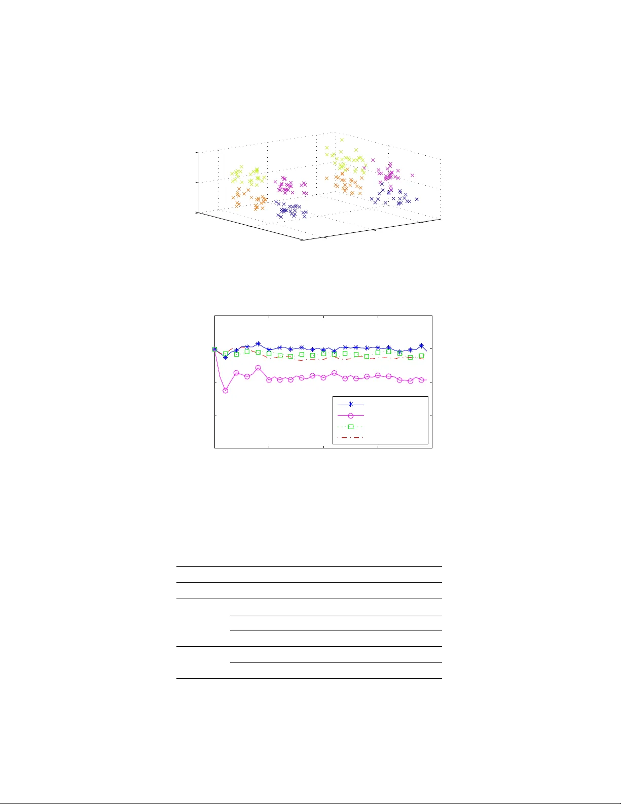
Adapti v e Evolutionary Clustering Ke vin S. Xu 1 , Mark Kliger 2 , and Alfred O. Hero III 1 1 EECS Department, Univ ersity of Michigan, Ann Arbor , MI, USA xukevin@umich.edu , hero@umich.edu 2 Omek Interactiv e, Israel, mark.kliger@gmail.com October 25, 2018 Abstract In many practical applications of clustering, the objects to be clustered ev olve ov er time, and a clustering result is desired at each time step. In such applications, e volutionary clustering typically outperforms traditional static clustering by producing clustering results that reﬂect long-term trends while being rob ust to short-term v ariations. Sev eral e volutionary clustering algo- rithms have recently been proposed, often by adding a temporal smoothness penalty to the cost function of a static clustering method. In this paper , we introduce a different approach to e volutionary clustering by accurately track- ing the time-varying proximities between objects followed by static cluster- ing. W e present an ev olutionary clustering framework that adaptiv ely esti- mates the optimal smoothing parameter using shrinkage estimation, a statis- tical approach that improv es a naïve estimate using additional information. The proposed framew ork can be used to e xtend a variety of static cluster- ing algorithms, including hierarchical, k-means, and spectral clustering, into ev olutionary clustering algorithms. Experiments on synthetic and real data sets indicate that the proposed framew ork outperforms static clustering and existing e volutionary clustering algorithms in man y scenarios. 1 Intr oduction In many practical applications of clustering, the objects to be clustered are ob- served at many points in time, and the goal is to obtain a clustering result at each time step. This situation arises in applications such as identifying communities in dynamic social networks (Falko wski et al., 2006; T antipathananandh et al., 2007), tracking groups of moving objects (Li et al., 2004; Carmi et al., 2009), ﬁnding time- v arying clusters of stocks or currencies in ﬁnancial mark ets (Fenn et al., 2009), and 1 many other applications in data mining, machine learning, and signal processing. T ypically the objects evolv e o ver time both as a result of long-term drifts due to changes in their statistical properties and short-term v ariations due to noise. A naïve approach to these types of problems is to perform static clustering at each time step using only the most recent data. This approach is extremely sensiti ve to noise and produces clustering results that are unstable and inconsistent with clustering results from adjacent time steps. Subsequently , e v olutionary clustering methods ha ve been de veloped, with the goal of producing clustering results that reﬂect long-term drifts in the objects while being robust to short-term v ariations 1 . Se veral ev olutionary clustering algorithms have recently been proposed by adding a temporal smoothness penalty to the cost function of a static clustering method. This penalty prev ents the clustering result at any given time from deviat- ing too much from the clustering results at neighboring time steps. This approach has produced e volutionary e xtensions of commonly used static clustering methods such as agglomerative hierarchical clustering (Chakrabarti et al., 2006), k-means (Chakrabarti et al., 2006), Gaussian mixture models (Zhang et al., 2009), and spec- tral clustering (T ang et al., 2008; Chi et al., 2009) among others. Ho w to choose the weight of the penalty in an optimal manner in practice, howe ver , remains an open problem. In this paper , we propose a dif ferent approach to e volutionary clustering by treating it as a problem of tracking followed by static clustering (Section 3). W e model the observed matrix of proximities between objects at each time step, which can be either similarities or dissimilarities, as a linear combination of a true pr ox- imity matrix and a zero-mean noise matrix. The true proximities, which vary over time, can be viewed as unobserved states of a dynamic system. Our approach in volv es estimating these states using both current and past proximities, then per- forming static clustering on the state estimates. The states are estimated using a restricted class of estimators kno wn as shrink- age estimators , which improve a raw estimate by combining it with other infor- mation. W e de velop a method for estimating the optimal weight to place on past proximities so as to minimize the mean squared error (MSE) between the true prox- imities and our estimates. W e call this weight the for getting factor . One advantage of our approach is that it provides an explicit formula for the optimal forgetting factor , unlik e existing e v olutionary clustering methods. The for getting factor is es- timated adaptively , which allo ws it to vary over time to adjust to the conditions of the dynamic system. The proposed framew ork, which we call Adapti ve For getting Factor for Evo- 1 The term “ev olutionary clustering” has also been used to refer to clustering algorithms moti vated by biological ev olution, which are unrelated to the methods discussed in this paper . 2 lutionary Clustering and T racking (AFFECT), can extend any static clustering al- gorithm that uses pairwise similarities or dissimilarities into an ev olutionary clus- tering algorithm. It is ﬂexible enough to handle changes in the number of clusters ov er time and to accommodate objects entering and leaving the data set between time steps. W e demonstrate how AFFECT can be used to extend three popular static clustering algorithms, namely hierarchical clustering, k-means, and spectral clustering, into ev olutionary clustering algorithms (Section 4). These algorithms are tested on sev eral synthetic and real data sets (Section 5). W e ﬁnd that they not only outperform static clustering, but also other recently proposed ev olutionary clustering algorithms due to the adapti vely selected forgetting f actor . The main contribution of this paper is the dev elopment of the AFFECT adap- ti ve ev olutionary clustering framew ork, which has se veral advantages ov er e xisting e volutionary clustering approaches: 1. It in volv es smoothing proximities between objects over time follo wed by static clustering, which enables it to extend any static clustering algorithm that takes a proximity matrix as input to an ev olutionary clustering algorithm. 2. It provides an explicit formula and estimation procedure for the optimal weight (forgetting f actor) to apply to past proximities. 3. It outperforms static clustering and existing ev olutionary clustering algo- rithms in several experiments with a minimal increase in computation time compared to static clustering (if a single iteration is used to estimate the for- getting factor). This paper is an extension of our previous work (Xu et al., 2010), which was limited to ev olutionary spectral clustering. In this paper , we extend the previously proposed framework to other static clustering algorithms. W e also provide addi- tional insight into the model assumptions in Xu et al. (2010) and demonstrate the ef fectiv eness of AFFECT in sev eral additional experiments. 2 Backgr ound 2.1 Static clustering algorithms W e begin by re viewing three commonly used static clustering algorithms. W e demonstrate the ev olutionary extension of these algorithms in Section 4, although the AFFECT framew ork can be used to extend many other static clustering algo- rithms. The term “clustering” is used in this paper to refer to both data clustering and graph clustering. The notation i ∈ c is used to denote object i being assigned to 3 1: Assign each object to its o wn cluster 2: r epeat 3: Compute dissimilarities between each pair of clusters 4: Merge clusters with the lo west dissimilarity 5: until all objects are mer ged into one cluster 6: r eturn dendrogram Figure 1: A general agglomerativ e hierarchical clustering algorithm. cluster c . | c | denotes the number of objects in cluster c , and C denotes a clustering result (the set of all clusters). In the case of data clustering, we assume that the n objects in the data set are stored in an n × p matrix X , where object i is represented by a p -dimensional feature vector x i corresponding to the i th row of X . From these feature vectors, one can create a proximity matrix W , where w ij denotes the proximity between objects i and j , which could be their Euclidean distance or any other similarity or dissimilarity measure. For graph clustering, we assume that the n v ertices in the graph are represented by an n × n adjacency matrix W where w ij denotes the weight of the edge between vertices i and j . If there is no edge between i and j , then w ij = 0 . For the usual case of undirected graphs with non-negati ve edge weights, an adjacency matrix is a similarity matrix, so we shall refer to it also as a proximity matrix. 2.1.1 Agglomerative hierar chical clustering Agglomerati ve hierarchical clustering algorithms are greedy algorithms that create a hierarchical clustering result, often represented by a dendrogram (Hastie et al., 2001). The dendrogram can be cut at a certain lev el to obtain a ﬂat clustering re- sult. There are many variants of agglomerativ e hierarchical clustering. A general algorithm is described in Fig. 1. V arying the deﬁnition of dissimilarity between a pair of clusters often changes the clustering results. Three common choices are to use the minimum dissimilarity between objects in the two clusters (single link- age), the maximum dissimilarity (complete linkage), or the average dissimilarity (av erage linkage) (Hastie et al., 2001). 4 1: i ← 0 2: C (0) ← vector of random inte gers in { 1 , . . . , k } 3: Compute similarity matrix W = X X T 4: r epeat 5: i ← i + 1 6: Calculate squared distance between all objects and centroids using (2) 7: Compute C ( i ) by assigning each object to its closest centroid 8: until C ( i ) = C ( i − 1) 9: r eturn C ( i ) Figure 2: Pseudocode for k-means clustering using similarity matrix W . 2.1.2 k-means k-means clustering (MacQueen, 1967; Hastie et al., 2001) attempts to ﬁnd clusters that minimize the sum of squares cost function D ( X, C ) = k X c =1 X i ∈ c k x i − m c k 2 , (1) where k · k denotes the ` 2 -norm, and m c is the centroid of cluster c , gi ven by m c = P i ∈ c x i | c | . Each object is assigned to the cluster with the closest centroid. The cost of a clustering result C is simply the sum of squared Euclidean distances between each object and its closest centroid. The squared distance in (1) can be rewritten as k x i − m c k 2 = w ii − 2 P j ∈ c w ij | c | + P j,l ∈ c w j l | c | 2 , (2) where w ij = x i x T j , the dot product of the feature vectors. Using the form of (2) to compute the k-means cost in (1) allows the k-means algorithm to be implemented with only the similarity matrix W = [ w ij ] n i,j =1 consisting of all pairs of dot prod- ucts, as described in Fig. 2. 2.1.3 Spectral clustering Spectral clustering (Shi and Malik, 2000; Ng et al., 2001; von Luxburg, 2007) is a popular modern clustering technique inspired by spectral graph theory . It can be used for both data and graph clustering. When used for data clustering, the ﬁrst step 5 1: Z ← k smallest eigen vectors of L 2: f or i = 1 to n do 3: z i ← z i / k z i k {Normalize each ro w of Z to hav e unit norm} 4: end f or 5: C ← kmeans( Z ) 6: r eturn C Figure 3: Pseudocode for normalized cut spectral clustering. in spectral clustering is to create a similarity graph with vertices corresponding to the objects and edge weights corresponding to the similarities between objects. W e represent the graph by an adjacency matrix W with edge weights w ij gi ven by a positi ve deﬁnite similarity function s ( x i , x j ) . The most commonly used similarity function is the Gaussian similarity function s ( x i , x j ) = exp {−k x i − x j k 2 / (2 ρ 2 ) } (Ng et al., 2001), where ρ is a scaling parameter . Let D denote a diagonal matrix with elements corresponding to row sums of W . Deﬁne the unnormalized graph Laplacian matrix by L = D − W and the normalized Laplacian matrix (Chung, 1997) by L = I − D − 1 / 2 W D − 1 / 2 . Three common variants of spectral clustering are av erage association (AA), ratio cut (RC), and normalized cut (NC) (Shi and Malik, 2000). Each variant is associated with an NP-hard graph optimization problem. Spectral clustering solv es relaxed versions of these problems. The relaxed problems can be written as (von Luxbur g, 2007; Chi et al., 2009) AA( Z ) = max Z ∈ R n × k tr( Z T W Z ) subject to Z T Z = I (3) R C( Z ) = min Z ∈ R n × k tr( Z T LZ ) subject to Z T Z = I (4) NC( Z ) = min Z ∈ R n × k tr( Z T L Z ) subject to Z T Z = I . (5) These are v ariants of a trace optimization problem; the solutions are giv en by a generalized Rayleigh-Ritz theorem (Lütkepohl, 1997). The optimal solution to (3) consists of the matrix containing the eigenv ectors corresponding to the k lar gest eigen v alues of W as columns. Similarly , the optimal solutions to (4) and (5) con- sist of the matrices containing the eigen vectors corresponding to the k smallest eigen v alues of L and L , respectiv ely . The optimal relaxed solution Z is then dis- cretized to obtain a clustering result, typically by running the standard k-means algorithm on the ro ws of Z or a normalized version of Z . An algorithm (Ng et al., 2001) for normalized cut spectral clustering is shown in Fig. 3. T o perform ratio cut spectral clustering, compute eigen vectors of L instead of L and ignore the row normalization in steps 2 – 4. Similarly , to perform 6 av erage association spectral clustering, compute instead the k largest eigen vectors of W and ignore the row normalization in steps 2 – 4. 2.2 Related work W e now summarize some contributions in the related areas of incremental and constrained clustering, as well as existing w ork on ev olutionary clustering. 2.2.1 Incremental clustering The term “incremental clustering” has typically been used to describe two types of clustering problems 2 : 1. Sequentially clustering objects that are each observed only once. 2. Clustering objects that are each observed o ver multiple time steps. T ype 1 is also known as data stream clustering, and the focus is on clustering the data in a single pass and with limited memory (Charikar et al., 2004; Gupta and Grossman, 2004). It is not directly related to our work because in data stream clustering each object is observed only once. T ype 2 is of greater rele v ance to our work and tar gets the same problem setting as ev olutionary clustering. Se veral incremental algorithms of this type have been proposed (Li et al., 2004; Sun et al., 2007; Ning et al., 2010). These incremental clustering algorithms could also be applied to the type of problems we consider; ho wev er , the focus of incremental clustering is on low computational cost at the expense of clustering quality . The incremental clustering result is often worse than the result of performing static clustering at each time step, which is already a sub- optimal approach as mentioned in the introduction. On the other hand, ev olutionary clustering is concerned with improving clustering quality by intelligently combin- ing data from multiple time steps and is capable of outperforming static clustering. 2.2.2 Constrained clustering The objecti ve of constrained clustering is to ﬁnd a clustering result that optimizes some goodness-of-ﬁt objective (such as the k-means sum of squares cost function (1)) subject to a set of constraints. The constraints can either be hard or soft. Hard constraints can be used, for example, to specify that two objects must or must not be in the same cluster (W agstaff et al., 2001; W ang and Davidson, 2010). On the 2 It is also sometimes used to refer to the simple approach of performing static clustering at each time step. 7 other hand, soft constraints can be used to specify real-v alued preferences, which may be obtained from labels or other prior information (Ji and Xu, 2006; W ang and Davidson, 2010). These soft constraints are similar to e volutionary clustering in that they bias clustering results based on additional information; in the case of e volutionary clustering, the additional information could correspond to historical data or clustering results. T adepalli et al. (2009) considered the problem of clustering time-ev olving ob- jects such that objects in the same cluster at a particular time step are unlikely to be in the same cluster at the following time step. Such an approach allows one to divide the time series into segments that differ signiﬁcantly from one another . Notice that this is the opposite of the ev olutionary clustering objectiv e, which fa- vors smooth ev olutions in cluster memberships ov er time. Hossain et al. (2010) proposed a framework that uniﬁes these two objectiv es, which are referred to as disparate and dependent clustering, respectively . Both can be viewed as clustering with soft constraints to minimize or maximize similarity between multiple sets of clusters, e.g. clusters at dif ferent time steps. 2.2.3 Evolutionary clustering The topic of ev olutionary clustering has attracted signiﬁcant attention in recent years. Chakrabarti et al. (2006) introduced the problem and proposed a general frame work for e volutionary clustering by adding a temporal smoothness penalty to a static clustering method. Evolutionary extensions for agglomerativ e hierarchical clustering and k-means were presented as examples of the frame work. Chi et al. (2009) expanded on this idea by proposing two frameworks for ev o- lutionary spectral clustering, which they called Preserving Cluster Quality (PCQ) and Preserving Cluster Membership (PCM). Both frameworks proposed to opti- mize the modiﬁed cost function C total = α C temporal + (1 − α ) C snapshot , (6) where C snapshot denotes the static spectral clustering cost, which is typically taken to be the av erage association, ratio cut, or normalized cut as discussed in Section 2.1.3. The tw o frameworks differ in how the temporal smoothness penalty C temporal is deﬁned. In PCQ, C temporal is deﬁned to be the cost of applying the clustering result at time t to the similarity matrix at time t − 1 . In other words, it penalizes clustering results that disagree with past similarities. In PCM, C temporal is deﬁned to be a measure of distance between the clustering results at time t and t − 1 . In other words, it penalizes clustering results that disagree with past clustering results. Both choices of temporal cost are quadratic in the cluster memberships, similar to the static spectral clustering cost as in (3)–(5), so optimizing (6) in either case is 8 simply a trace optimization problem. For example, the PCQ av erage association e volutionary spectral clustering problem is gi ven by max Z ∈ R n × k α tr  Z T W t − 1 Z  + (1 − α ) tr  Z T W t Z  subject to Z T Z = I , where W t and W t − 1 denote the adjacency matrices at times t and t − 1 , respec- ti vely . The PCQ cluster memberships can be found by computing eigenv ectors of αW t − 1 + (1 − α ) W t and then discretizing as discussed in Section 2.1.3. Our work takes a different approach than that of Chi et al. (2009) b ut the resulting frame work shares some similarities with the PCQ framew ork. In particular, AFFECT paired with average association spectral clustering is an extension of PCQ to longer his- tory , which we discuss in Section 4.3. Follo wing these works, other ev olutionary clustering algorithms that attempt to optimize the modiﬁed cost function deﬁned in (6) ha ve been proposed (T ang et al., 2008; Lin et al., 2009; Zhang et al., 2009; Mucha et al., 2010). The deﬁnitions of snapshot and temporal cost and the clustering algorithms vary by approach. None of the aforementioned works addresses the problem of ho w to choose the parameter α in (6), which determines ho w much weight to place on historic data or clustering results. It has typically been suggested (Chi et al., 2009; Lin et al., 2009) to choose it in an ad-hoc manner according to the user’ s subjectiv e preference on the temporal smoothness of the clustering results. It could also be beneﬁcial to allow α to v ary with time. Zhang et al. (2009) proposed to choose α adaptively by using a test statistic for checking dependency between two data sets (Gretton et al., 2007). Howe ver , this test statistic also does not satisfy any optimality properties for ev olutionary clustering and still depends on a global parameter reﬂecting the user’ s preference on temporal smoothness, which is undesirable. The existing method that is most similar to AFFECT is that of Rosswog and Ghose (2008), which we refer to as RG. The authors proposed e volutionary exten- sions of k-means and agglomerativ e hierarchical clustering by ﬁltering the feature vectors using a Finite Impulse Response (FIR) ﬁlter , which combines the last l + 1 measurements of the feature vectors by the weighted sum y t i = b 0 x t i + b 1 x t − 1 i + · · · + b l x t − l i , where l is the order of the ﬁlter , y t i is the ﬁlter output at time t , and b 0 , . . . , b l are the ﬁlter coef ﬁcients. The proximities are then calculated between the ﬁlter outputs rather than the feature vectors. The main resemblance between RG and AFFECT is that RG is also based on tracking followed by static clustering. In particular , RG adapti vely selects the ﬁlter coefﬁcients based on the dissimilarities between cluster centroids at the past l time steps. Howe ver , RG cannot accommo- date varying numbers of clusters over time nor can it deal with objects entering and leaving at v arious time steps. It also struggles to adapt to changes in clusters, as we 9 demonstrate in Section 5.2. AFFECT , on the other hand, is able to adapt quickly to changes in clusters and is applicable to a much larger class of problems. Finally , there has also been recent interest in model-based e volutionary cluster- ing. In addition to the aforementioned method in volving mixtures of exponential families (Zhang et al., 2009), methods hav e also been proposed using semi-Marko v models (W ang et al., 2007), Dirichlet process mixtures (DPMs) (Ahmed and Xing, 2008; Xu et al., 2008b), hierarchical DPMs (Xu et al., 2008b,a; Zhang et al., 2010), and smooth plaid models (Mankad et al., 2011). For these methods, the temporal e volution is controlled by hyperparameters that can be estimated in some cases. 3 Pr oposed evolutionary framew ork The proposed framework treats ev olutionary clustering as a tracking problem fol- lo wed by ordinary static clustering. In the case of data clustering, we assume that the feature vectors have already been con verted into a proximity matrix, as discussed in Section 2.1. W e treat the proximity matrices, denoted by W t , as re- alizations from a non-stationary random process indexed by discrete time steps, denoted by the superscript t . W e assume, like many other e volutionary cluster- ing algorithms, that the identities of the objects can be tracked ov er time so that the ro ws and columns of W t correspond to the same objects as those of W t − 1 provided that no objects are added or removed (we describe how the proposed framew ork handles adding and removing objects in Section 4.4.1). Furthermore we posit the linear observ ation model W t = Ψ t + N t , t = 0 , 1 , 2 , . . . (7) where Ψ t is an unknown deterministic matrix of unobserved states, and N t is a zero-mean noise matrix. Ψ t changes ov er time to reﬂect long-term drifts in the proximities. W e refer to Ψ t as the true pr oximity matrix , and our goal is to ac- curately estimate it at each time step. On the other hand, N t reﬂects short-term v ariations due to noise. Thus we assume that N t , N t − 1 , . . . , N 0 are mutually in- dependent. A common approach for tracking unobserved states in a dynamic system is to use a Kalman ﬁlter (Harv ey, 1989; Haykin, 2001) or some variant. Since the states correspond to the true proximities, there are O ( n 2 ) states and O ( n 2 ) observ ations, which mak es the Kalman ﬁlter impractical for tw o reasons. First, it in volves speci- fying a parametric model for the state e v olution o ver time, and secondly , it requires the in version of an O ( n 2 ) × O ( n 2 ) cov ariance matrix, which is large enough in most e volutionary clustering applications to make matrix inv ersion computation- ally infeasible. W e present a simpler approach that inv olves a recursiv e update of 10 the state estimates using only a single parameter α t , which we deﬁne in (8). 3.1 Smoothed proximity matrix If the true proximity matrix Ψ t is known, we would expect to see improved cluster- ing results by performing static clustering on Ψ t rather than on the current proxim- ity matrix W t because Ψ t is free from noise. Our objectiv e is to accurately estimate Ψ t at each time step. W e can then perform static clustering on our estimate, which should also lead to improv ed clustering results. The naïve approach of performing static clustering on W t at each time step can be interpreted as using W t itself as an estimate for Ψ t . The main disadv antage of this approach is that it suffers from high v ariance due to the observation noise N t . As a consequence, the obtained clustering results can be highly unstable and inconsistent with clustering results from adjacent time steps. A better estimate can be obtained using the smoothed pr oximity matrix ˆ Ψ t de- ﬁned by ˆ Ψ t = α t ˆ Ψ t − 1 + (1 − α t ) W t (8) for t ≥ 1 and by ˆ Ψ 0 = W 0 . Notice that ˆ Ψ t is a function of current and past data only , so it can be computed in the on-line setting where a clustering result for time t is desired before data at time t + 1 can be obtained. ˆ Ψ t incorporates proximities not only from time t − 1 , but potentially from all previous time steps and allows us to suppress the observation noise. The parameter α t controls the rate at which past proximities are forgotten; hence we refer to it as the for getting factor . The forgetting factor in our framew ork can change over time, allowing the amount of temporal smoothing to v ary . 3.2 Shrinkage estimation of true proximity matrix The smoothed proximity matrix ˆ Ψ t is a natural candidate for estimating Ψ t . It is a con vex combination of two estimators: W t and ˆ Ψ t − 1 . Since N t is zero-mean, W t is an unbiased estimator but has high v ariance because it uses only a single observ ation. ˆ Ψ t − 1 is a weighted combination of past observations so it should hav e lo wer v ariance than W t , b ut it is likely to be biased since the past proximities may not be representativ e of the current ones as a result of long-term drift in the statistical properties of the objects. Thus the problem of estimating the optimal forgetting f actor α t may be considered as a bias-v ariance trade-off problem. A similar bias-variance trade-off has been in vestigated in the problem of shrink- age estimation of cov ariance matrices (Ledoit and W olf, 2003; Schäfer and Strim- mer, 2005; Chen et al., 2010), where a shrinkage estimate of the cov ariance matrix is taken to be ˆ Σ = λT + (1 − λ ) S , a con ve x combination of a suitably chosen target 11 matrix T and the standard estimate, the sample cov ariance matrix S . Notice that the shrinkage estimate has the same form as the smoothed proximity matrix giv en by (8) where the smoothed proximity matrix at the previous time step ˆ Ψ t − 1 cor- responds to the shrinkage target T , the current proximity matrix W t corresponds to the sample cov ariance matrix S , and α t corresponds to the shrinkage intensity λ . W e deriv e the optimal choice of α t in a manner similar to Ledoit and W olf ’ s deri vation of the optimal λ for shrinkage estimation of covariance matrices (Ledoit and W olf, 2003). As in Ledoit and W olf (2003), Schäfer and Strimmer (2005), and Chen et al. (2010), we choose to minimize the squared Frobenius norm of the difference be- tween the true proximity matrix and the smoothed proximity matrix. That is, we take the loss function to be L  α t  =    ˆ Ψ t − Ψ t    2 F = n X i =1 n X j =1  ˆ ψ t ij − ψ t ij  2 . W e deﬁne the risk to be the conditional expectation of the loss function given all of the pre vious observations R  α t  = E     ˆ Ψ t − Ψ t    2 F     W ( t − 1)  where W ( t − 1) denotes the set  W t − 1 , W t − 2 , . . . , W 0  . Note that the risk function is differentiable and can be easily optimized if Ψ t is known. Howe ver , Ψ t is the quantity that we are trying to estimate so it is not known. W e ﬁrst deri ve the optimal for getting factor assuming it is kno wn. W e shall henceforth refer to this as the oracle for getting factor . Under the linear observ ation model of (7), E h W t   W ( t − 1) i = E  W t  = Ψ t (9) v ar  W t   W ( t − 1)  = v ar  W t  = v ar  N t  (10) because N t , N t − 1 , . . . , N 0 are mutually independent and have zero mean. From the deﬁnition of ˆ Ψ t in (8), the risk can then be expressed as R  α t  = n X i =1 n X j =1 E   α t ˆ ψ t − 1 ij +  1 − α t  w t ij − ψ t ij  2     W ( t − 1)  = n X i =1 n X j =1  v ar  α t ˆ ψ t − 1 ij +  1 − α t  w t ij − ψ t ij    W ( t − 1)  + E h α t ˆ ψ t − 1 ij +  1 − α t  w t ij − ψ t ij    W ( t − 1) i 2  . (11) 12 (11) can be simpliﬁed using (9) and (10) and by noting that the conditional variance of ˆ ψ t − 1 ij is zero and that ψ t ij is deterministic. Thus R  α t  = n X i =1 n X j =1   1 − α t  2 v ar  n t ij  +  α t  2  ˆ ψ t − 1 ij − ψ t ij  2  . (12) From (12), the ﬁrst deri vati ve is easily seen to be R 0  α t  = 2 n X i =1 n X j =1   α t − 1  v ar  n t ij  + α t  ˆ ψ t − 1 ij − ψ t ij  2  . T o determine the oracle for getting factor  α t  ∗ , simply set R 0  α t  = 0 . Rearrang- ing to isolate α t , we obtain  α t  ∗ = n X i =1 n X j =1 v ar  n t ij  n X i =1 n X j =1   ˆ ψ t − 1 ij − ψ t ij  2 + v ar  n t ij   . (13) W e ﬁnd that  α t  ∗ does indeed minimize the risk because R 00  α t  ≥ 0 for all α t . The oracle forgetting factor  α t  ∗ leads to the best estimate in terms of mini- mizing risk but is not implementable because it requires oracle kno wledge of the true proximity matrix Ψ t , which is what we are trying to estimate, as well as the noise v ariance v ar  N t  . It was suggested in Schäfer and Strimmer (2005) to re- place the unknowns with their sample equiv alents. In this setting, we would replace ψ t ij with the sample mean of w t ij and v ar( n t ij ) = v ar( w t ij ) with the sample vari- ance of w t ij . Howe ver , Ψ t and potentially v ar  N t  are time-varying so we cannot simply use the temporal sample mean and v ariance. Instead, we propose to use the spatial sample mean and v ariance. Since objects belong to clusters, it is reasonable to assume that the structure of Ψ t and v ar  N t  should reﬂect the cluster member - ships. Hence we make an assumption about the structure of Ψ t and v ar  N t  in order to proceed. 3.3 Block model f or true proximity matrix W e propose a block model for the true proximity matrix Ψ t and v ar  N t  and use the assumptions of this model to compute the desired sample means and v ariances. The assumptions of the block model are as follo ws: 1. ψ t ii = ψ t j j for any tw o objects i, j that belong to the same cluster . 13 Figure 4: Block structure of true proximity matrix Ψ t . ψ t ( c ) denotes ψ t ii for all objects i in cluster c , and ψ t ( cd ) denotes ψ t ij for all distinct objects i, j such that i is in cluster c and j is in cluster d . 2. ψ t ij = ψ t lm for any two distinct objects i, j and any two distinct objects l , m such that i, l belong to the same cluster , and j, m belong to the same cluster . The structure of the true proximity matrix Ψ t under these assumptions is sho wn in Fig. 4. In short, we are assuming that the true proximity is equal inside the clusters and different between clusters. W e make the assumptions on v ar  N t  that we do on Ψ t , namely that it also possesses the assumed block structure. One scenario where the block assumptions are completely satisﬁed is the case where the data at each time t are realizations from a dynamic Gaussian mixture model (GMM) (Carmi et al., 2009), which is described as follows. Assume that the k components of the dynamic GMM are parameterized by the k time-varying mean vectors  µ t c  k c =1 and cov ariance matrices  Σ t c  k c =1 . Let { φ c } k c =1 denote the mixture weights. Objects are sampled in the following manner: 1. (Only at t = 0 ) Draw n samples { z i } n i =1 from the categorical distribution speciﬁed by { φ c } k c =1 to determine the component membership of each ob- ject. 2. (For all t ) For each object i , draw a sample x t i from the Gaussian distribution parameterized by  µ t z i , Σ t z i  . Notice that while the parameters of the individual components change ov er time, the component memberships do not, i.e. objects stay in the same components over time. The dynamic GMM simulates clusters moving in time. In Appendix A, we 14 sho w that at each time t , the mean and variance of the dot product similarity ma- trix W t , which correspond to Ψ t and v ar  N t  respecti vely under the observation model of (7), do indeed satisfy the assumed block structure. This scenario forms the basis of the experiment in Section 5.1. Although the proposed block model is rather simplistic, we believe that it is a reasonable choice when there is no prior information about the shapes of clusters. A similar block assumption has also been used in the dynamic stochastic block model (Y ang et al., 2011), developed for modeling dynamic social networks. A nice feature of the proposed block model is that it is permutation in variant with respect to the clusters; that is, it does not require objects to be ordered in any particular manner . The extension of the proposed framew ork to other models is beyond the scope of this paper and is an area for future w ork. 3.4 Adaptive estimation of f orgetting factor Under the block model assumption, the means and variances of proximities are identical in each block. As a result, we can sample over all proximities in a block to obtain sample means and variances. Unfortunately , we do not know the true block structure because the cluster memberships are unkno wn. T o work around this problem, we estimate the cluster memberships along with  α t  ∗ in an iterati ve fashion. First we initialize the cluster memberships. T wo log- ical choices are to use the cluster memberships from the previous time step or the memberships obtained from performing static clustering on the current proximities. W e can then sample over each block to estimate the entries of Ψ t and v ar  N t  as detailed below , and substitute them into (13) to obtain an estimate  ˆ α t  ∗ of  α t  ∗ . No w substitute  ˆ α t  ∗ into (8) and perform static clustering on ˆ Ψ t to obtain an up- dated clustering result. This clustering result is then used to reﬁne the estimate of  α t  ∗ , and this iterati ve process is repeated to impro ve the quality of the clustering result. W e ﬁnd, empirically , that the estimated forgetting factor rarely changes after the third iteration and that e ven a single iteration often provides a good estimate. T o estimate the entries of Ψ t = E  W t  , we proceed as follows. F or two distinct objects i and j both in cluster c , we estimate ψ t ij using the sample mean b E  w t ij  = 1 | c | ( | c | − 1) X l ∈ c X m ∈ c m 6 = l w t lm . Similarly , we estimate ψ t ii by b E  w t ii  = 1 | c | X l ∈ c w t ll . 15 1: C t ← C t − 1 2: f or i = 1 , 2 , . . . do {iteration number} 3: Compute b E  W t  and c v ar  W t  using C t 4: Calculate  ˆ α t  ∗ by substituting estimates b E  W t  and c v ar  W t  into (13) 5: ˆ Ψ t ←  ˆ α t  ∗ ˆ Ψ t − 1 +  1 −  ˆ α t  ∗  W t 6: C t ← cluster( ˆ Ψ t ) 7: end f or 8: r eturn C t Figure 5: Pseudocode for generic AFFECT ev olutionary clustering algorithm. Cluster( · ) denotes any static clustering algorithm that takes a similarity or dis- similarity matrix as input and returns a ﬂat clustering result. For distinct objects i in cluster c and j in cluster d with c 6 = d , we estimate ψ t ij by b E  w t ij  = 1 | c || d | X l ∈ c X m ∈ d w t lm . v ar  N t  = v ar  W t  can be estimated in a similar manner by taking unbiased sample v ariances over the blocks. 4 Evolutionary algorithms From the deriv ation in Section 3.4, we have the generic algorithm for AFFECT at each time step shown in Fig. 5. W e provide some details and interpretation of this generic algorithm when used with three popular static clustering algorithms: agglomerati ve hierarchical clustering, k-means, and spectral clustering. 4.1 Agglomerative hierar chical clustering The proposed ev olutionary extension of agglomerati ve hierarchical clustering has an interesting interpretation in terms of the modiﬁed cost function deﬁned in (6). Recall that agglomerativ e hierarchical clustering is a greedy algorithm that mer ges the two clusters with the lowest dissimilarity at each iteration. The dissimilarity between two clusters can be interpreted as the cost of merging them. Thus, per- forming agglomerati ve hierarchical clustering on ˆ Ψ t results in merging the two clusters with the lowest modiﬁed cost at each iteration. The snapshot cost of a merge corresponds to the cost of making the merge at time t using the dissimi- larities giv en by W t . The temporal cost of a merge is a weighted combination of 16 the costs of making the merge at each time step s ∈ { 0 , 1 , . . . , t − 1 } using the dissimilarities giv en by W s . This can be seen by expanding the recursi ve update in (8) to obtain ˆ Ψ t =  1 − α t  W t + α t  1 − α t − 1  W t − 1 + α t α t − 1  1 − α t − 2  W t − 2 + · · · + α t α t − 1 · · · α 2  1 − α 1  W 1 + α t α t − 1 · · · α 2 α 1 W 0 . (14) 4.2 k-means k-means is an iterati ve clustering algorithm and requires an initial set of cluster memberships to begin the iteration. In static k-means, typically a random initial- ization is employed. A good initialization can signiﬁcantly speed up the algorithm by reducing the number of iterations required for con ver gence. For ev olutionary k- means, an obvious choice is to initialize using the clustering result at the previous time step. W e use this initialization in our experiments in Section 5. The proposed ev olutionary k-means algorithm can also be interpreted as opti- mizing the modiﬁed cost function of (6). The snapshot cost is D  X t , C t  where D ( · , · ) is the sum of squares cost deﬁned in (1). The temporal cost is a weighted combination of D  X t , C s  , s ∈ { 0 , 1 , . . . , t − 1 } , i.e. the cost of the clustering result applied to the data at time s . Hence the modiﬁed cost measures ho w well the current clustering result ﬁts both current and past data. 4.3 Spectral clustering The proposed ev olutionary av erage association spectral clustering algorithm in- volv es computing and discretizing eigen vectors of ˆ Ψ t rather than W t . It can also be interpreted in terms of the modiﬁed cost function of (6). Recall that the cost in static av erage association spectral clustering is tr  Z T W Z  . Performing average association spectral clustering on ˆ Ψ t optimizes tr Z T " t X s =0 β s W s # Z ! = t X s =0 β s tr  Z T W s Z  , (15) where β s corresponds to the coefﬁcient in front of W s in (14). Thus, the snapshot cost is simply tr  Z T W t Z  while the temporal cost corresponds to the remaining t terms in (15). W e note that in the case where α t − 1 = 0 , this modiﬁed cost is identical to that of PCQ, which incorporates historical data from time t − 1 only . Hence our proposed generic frame work reduces to PCQ in this special case. Chi et al. (2009) noted that PCQ can easily be extended to accommodate longer history and suggested to do so by using a constant exponentially weighted forget- ting factor . Our proposed framew ork uses an adapti ve forgetting factor , which 17 Objects to be removed New objects Figure 6: Adding and removing objects over time. Shaded ro ws and columns are to be removed before computing ˆ Ψ t . The rows and columns for the ne w objects are then appended to ˆ Ψ t . should improve clustering performance, especially if the rate at which the statisti- cal properties of the data are e volving is time-v arying. Evolutionary ratio cut and normalized cut spectral clustering can be performed by forming the appropriate graph Laplacian, L t or L t , respectively , using ˆ Ψ t in- stead of W t . They do not admit any obvious interpretation in terms of a modiﬁed cost function since they operate on L t and L t rather than W t . 4.4 Practical issues 4.4.1 Adding and remo ving objects over time Up to this point, we ha ve assumed that the same objects are being observed at multiple time steps. In many application scenarios, ho wev er , new objects are often introduced over time while some existing objects may no longer be observed. In such a scenario, the indices of the proximity matrices W t and ˆ Ψ t − 1 correspond to dif ferent objects, so one cannot simply combine them as described in (8). These types of scenarios can be dealt with in the following manner . Objects that were observed at time t − 1 but not at time t can simply be remo ved from ˆ Ψ t − 1 in (8). New objects introduced at time t have no corresponding rows and columns in ˆ Ψ t − 1 . These new objects can be naturally handled by adding rows and columns to ˆ Ψ t after performing the smoothing operation in (8). In this way , the new nodes hav e no inﬂuence on the update of the forgetting factor α t yet contribute to the clustering result through ˆ Ψ t . This process is illustrated graphically in Fig. 6. 18 4.4.2 Selecting the number of clusters The task of optimally choosing the number of clusters at each time step is a dif ﬁcult model selection problem that is be yond the scope of this paper . Howe ver , since the proposed framework inv olves simply forming a smoothed proximity matrix fol- lo wed by static clustering, heuristics used for selecting the number of clusters in static clustering can also be used with the proposed ev olutionary clustering frame- work. One such heuristic applicable to many clustering algorithms is to choose the number of clusters to maximize the average silhouette width (Rousseeuw, 1987). For hierarchical clustering, selection of the number of clusters is often accom- plished using a stopping rule; a revie w of man y such rules can be found in Millig an and Cooper (1985). The eigengap heuristic (von Luxb urg, 2007) and the modular- ity criterion (Newman, 2006) are commonly used heuristics for spectral clustering. Any of these heuristics can be employed at each time step to choose the number of clusters, which can change ov er time. 4.4.3 Matching clusters between time steps While the AFFECT framew ork provides a clustering result at each time that is consistent with past results, one still faces the challenge of matching clusters at time t with those at times t − 1 and earlier . This requires permuting the clusters in the clustering result at time t . If a one-to-one cluster matching is desired, then the cluster matching problem can be formulated as a maximum weight matching between the clusters at time t and those at time t − 1 with weights corresponding to the number of common objects between clusters. The maximum weight matching can be found in polynomial time using the Hungarian algorithm (Kuhn, 1955). The more general cases of many-to-one (multiple clusters being merged into a single cluster) and one-to-many (a cluster splitting into multiple clusters) matching are beyond the scope of this paper . W e refer interested readers to Greene et al. (2010) and Bródka et al. (2012), both of which speciﬁcally address the cluster matching problem. 5 Experiments W e in vestigate the performance of the proposed AFFECT framew ork in ﬁv e ex- periments in volving both synthetic and real data sets. Tracking performance is measured in terms of the MSE E h k ˆ Ψ t − Ψ t k 2 F i , which is the criterion we seek to optimize. Clustering performance is measured by the Rand index (Rand, 1971), which is a quantity between 0 and 1 that indicates the amount of agreement between a clustering result and a set of labels, which are taken to be the ground truth. A 19 0 10 20 30 40 10 3 10 4 10 5 Time step MSE Covariance changed Estimated α t Oracle α t Static α t = 0.25 α t = 0.5 α t = 0.75 Figure 7: Comparison of MSE in well-separated Gaussians experiment. The adap- ti vely estimated forgetting factor outperforms the constant forgetting factors and achie ves MSE very close to the oracle for getting factor . higher Rand index indicates higher agreement, with a Rand index of 1 correspond- ing to perfect agreement. W e run at least one experiment for each of hierarchical clustering, k-means, and spectral clustering and compare the performance of AF- FECT against three recently proposed ev olutionary clustering methods discussed in Section 2.2.3: RG, PCQ, and PCM. W e run three iterations of AFFECT unless otherwise speciﬁed. 5.1 W ell-separated Gaussians This experiment is designed to test the tracking ability of AFFECT . W e draw 40 samples equally from a mixture of two 2 -D Gaussian distributions with mean vectors (4 , 0) and ( − 4 , 0) and with both cov ariance matrices equal to 0 . 1 I . At each time step, the means of the two distributions are moved according to a one- dimensional random walk in the ﬁrst dimension with step size 0 . 1 , and a ne w sam- ple is drawn with the component memberships ﬁxed, as described in Section 3.3. At time 19 , we change the cov ariance matrices to 0 . 3 I to test ho w well the frame- work can respond to a sudden change. W e run this e xperiment 100 times over 40 time steps using ev olutionary k- means clustering. The two clusters are well-separated so e ven static clustering is able to correctly identify them. Ho we ver the tracking performance is improved signiﬁcantly by incorporating historical data, which can be seen in Fig. 7 where the MSE between the estimated and true similarity matrices is plotted for sev eral choices of forgetting factor , including the estimated α t . W e also compare to the oracle α t , which can be calculated using the true moments and cluster memberships 20 0 10 20 30 40 0 0.2 0.4 0.6 0.8 1 Time step α t Covariance changed Estimated α t Oracle α t (a) 40 samples 0 10 20 30 40 0 0.2 0.4 0.6 0.8 1 Time step α t Covariance changed Estimated α t Oracle α t (b) 200 samples Figure 8: Comparison of oracle and estimated forgetting factors in well-separated Gaussians experiment. The gap between the estimated and oracle forgetting factors decreases as the sample size increases. of the data as sho wn in Appendix A but is not implementable in a real application. Notice that the estimated α t performs very well, and its MSE is very close to that of the oracle α t . The estimated α t also outperforms all of the constant forgetting factors. The estimated α t is plotted as a function of time in Fig. 8(a). Since the clusters are well-separated, only a single iteration is performed to estimate α t . Notice that both the oracle and estimated forgetting factors quickly increase from 0 then lev el of f to a nearly constant value until time 19 when the cov ariance matrix is changed. After the transient due to the change in covariance, both the oracle and estimated forgetting factors again level off. This behavior is to be expected because the two clusters are moving according to random walks. Notice that the estimated α t does not con verge to the same value the oracle α t appears to. This bias is due to the ﬁnite sample size. The estimated and oracle for getting factors are plotted in Fig. 8(b) for the same experiment but with 200 samples rather than 40 . The gap between the steady-state values of the estimated and oracle forgetting factors is much smaller no w , and it continues to decrease as the sample size increases. 5.2 T wo colliding Gaussians The objecti ve of this experiment is to test the effecti veness of the AFFECT frame- work when a cluster moves close enough to another cluster so that they ov erlap. W e also test the ability of the frame work to adapt to a change in cluster membership. The setup of this experiment is illustrated in Fig. 9. W e draw 40 samples from a mixture of two 2 -D Gaussian distributions, both with covariance matrix equal to 21 −6 −4 −2 0 2 4 6 −6 −4 −2 0 2 4 6 Figure 9: Setup of two colliding Gaussians experiment: one cluster is slowly mov ed tow ard the other , then a change in cluster membership is simulated. identity . The mixture proportion (the proportion of samples dra wn from the second cluster) is initially chosen to be 1 / 2 . The ﬁrst cluster has mean (3 , 3) and remains stationary throughout the experiment. The second cluster’ s mean is initially at ( − 3 , − 3) and is mov ed toward the ﬁrst cluster from time steps 0 to 9 by (0 . 4 , 0 . 4) at each time. At times 10 and 11 , we switch the mixture proportion to 3 / 8 and 1 / 4 , respecti vely , to simulate objects changing cluster . From time 12 onwards, both the cluster means and mixture proportion are unchanged. At each time, we draw a new sample. W e run this experiment 100 times using ev olutionary k-means clustering. The MSE in this experiment for varying α t is shown in Fig. 10. As before, the ora- cle α t is calculated using the true moments and cluster memberships and is not implementable in practice. It can be seen that the choice of α t af fects the MSE signiﬁcantly . The estimated α t performs the best, excluding the oracle α t , which is not implementable. Notice also that α t = 0 . 5 performs well before the change in cluster memberships at time 10 , i.e. when cluster 2 is moving, while α t = 0 . 75 performs better after the change when both clusters are stationary . The clustering accuracy for this experiment is plotted in Fig. 11. Since this experiment in volv es k-means clustering, we compare to the RG method. W e simu- late two ﬁlter lengths for RG: a short-memory 3 rd-order ﬁlter and a long-memory 10 th-order ﬁlter . In Fig. 11 it can be seen that the estimated α t also performs best in Rand index, approaching the performance of the oracle α t . The static method performs poorly as soon as the clusters begin to ov erlap at around time step 7 . All of the e volutionary methods handle the ov erlap well, b ut the RG method is slo w to respond to the change in clusters, especially the long-memory ﬁlter . In T able 1, we 22 0 5 10 15 20 25 10 3 10 4 10 5 10 6 Time step MSE Change 1 Change 2 Estimated α t Oracle α t Static α t = 0.25 α t = 0.5 α t = 0.75 Figure 10: Comparison of MSE in two colliding Gaussians experiment. The esti- mated α t performs best both before and after the change points. 0 5 10 15 20 25 0.5 0.6 0.7 0.8 0.9 1 Time step Rand index Change 1 Change 2 Estimated α t Oracle α t Static RG (3rd order) RG (10th order) Figure 11: Comparison of Rand index in two colliding Gaussians experiment. The estimated α t detects the changes in clusters quickly unlike the RG method. 23 T able 1: Means and standard errors of k-means Rand indices in two colliding Gaus- sians e xperiment. Bolded number indicates best performer within one standard error . Method Parameters Rand index Static - 0 . 899 ± 0 . 002 AFFECT Estimated α t ( 3 iterations) 0 . 984 ± 0 . 001 Estimated α t ( 1 iteration) 0 . 978 ± 0 . 001 α t = 0 . 5 0 . 975 ± 0 . 001 RG l = 3 0 . 955 ± 0 . 001 l = 10 0 . 861 ± 0 . 001 0 5 10 15 20 25 0 0.2 0.4 0.6 0.8 1 Time step α t Change 1 Change 2 1st iteration 2nd iteration 3rd iteration 4th iteration 5th iteration Oracle α t Figure 12: Comparison of oracle and estimated forgetting factors in two colliding Gaussians experiment. There is no noticeable change after the third iteration. present the means and standard errors (o ver the simulation runs) of the mean Rand indices of each method over all time steps. For AFFECT , we also show the Rand index when only one iteration is used to estimate α t and when arbitrarily setting α t = 0 . 5 , both of which also outperform the RG method in this experiment. The poorer performance of the RG method is to be e xpected because it places more weight on time steps where the cluster centroids are well-separated, which again results in too much weight on historical data after the cluster memberships are changed. The estimated α t is plotted by iteration in Fig. 12 along with the oracle α t . Notice that the estimate gets better over the ﬁrst three iterations, while the fourth and ﬁfth show no visible improv ement. The plot of the estimated α t suggests why it is able to outperform the constant α t ’ s. It is almost constant at the beginning of 24 the experiment when the second cluster is moving, then it decreases over the two times when cluster memberships are changed, and ﬁnally it increases when the two clusters are both stationary . The values of the oracle α t before and after the change corroborate the pre vious observation that α t = 0 . 5 performs well before the change, b ut α t = 0 . 75 performs better afterwards. Notice that the estimated α t appears to conv erge to a lower value than the oracle α t . This is once again due to the ﬁnite-sample ef fect discussed in Section 5.1. 5.3 Flocks of boids This experiment in volves simulation of a natural phenomenon, namely the ﬂocking behavior of birds. T o simulate this phenomenon we use the bird-oid objects (boids) model proposed by Reynolds (1987). The boids model allo ws us to simulate natural mov ements of objects and clusters. The beha vior of the boids are governed by three main rules: 1. Boids try to ﬂy to wards the av erage position (centroid) of local ﬂock mates. 2. Boids try to keep a small distance a way from other boids. 3. Boids try to ﬂy to wards the av erage heading of local ﬂock mates. Our implementation of the boids model is based on the pseudocode of Parker (2007). At each time step, we mov e each boid 1 / 100 of the way tow ards the av er- age position of local ﬂock mates, double the distance between boids that are within 10 units of each other, and move each boid 1 / 8 of the way towards the average heading. W e run two experiments using the boids model; one with a ﬁxed number of ﬂocks ov er time and one where the number of ﬂocks varies o ver time. 5.3.1 Fixed number of ﬂocks Four ﬂocks of 25 boids are initially distrib uted uniformly in separate 60 × 60 × 60 cubes. T o simulate boids moving continuously in time while being observed at regular time interv als, we allow each boid to perform ﬁve movements per time step according to the aforementioned rules. Similar to Reynolds (1987), we use goal setting to push the ﬂocks along parallel paths. Note that unlike in the previous experiments, the ﬂocking beha vior makes it possible to simulate natural changes in cluster , simply by changing the ﬂock membership of a boid. W e change the ﬂock memberships of a randomly selected boid at each time step. The initial and ﬁnal positions of the ﬂocks for one realization are sho wn in Fig. 13. 25 0 500 1000 −100 0 100 −100 0 100 Figure 13: Setup of boids experiment: four ﬂocks ﬂy along parallel paths (start and end positions sho wn). At each time step, a randomly selected boid joins one of the other ﬂocks. 0 10 20 30 40 0.8 0.85 0.9 0.95 1 Time step Rand index Estimated α t Static RG (3rd order) RG (10th order) Figure 14: Comparison of complete linkage Rand index in boids experiment. The estimated α t performs much better than static clustering and slightly better than the RG method. T able 2: Means and standard errors of complete linkage Rand indices in boids experiment. Method Parameters Rand index Static - 0 . 908 ± 0 . 001 AFFECT Estimated α t ( 3 iterations) 0 . 950 ± 0 . 001 Estimated α t ( 1 iteration) 0 . 945 ± 0 . 001 α t = 0 . 5 0 . 945 ± 0 . 001 RG l = 3 0 . 942 ± 0 . 001 l = 10 0 . 939 ± 0 . 000 26 W e run this experiment 100 times using complete linkage hierarchical cluster- ing. Unlike in the pre vious e xperiments, we do not kno w the true proximity matrix so MSE cannot be calculated. Clustering accuracy , ho wev er , can still be computed using the true ﬂock memberships. The clustering performance of the v arious ap- proaches is displayed in Fig. 14. Notice that AFFECT once again performs better than RG, both with short and long memory , although the difference is much smaller than in the two colliding Gaussians experiment. The means and standard errors of the Rand indices for the various methods are listed in T able 2. Again, it can be seen that AFFECT is the best performer . The estimated α t in this experiment is roughly constant at around 0 . 6 . This is not a surprise because all mov ements in this experi- ment, including changes in clusters, are smooth as a result of the ﬂocking motions of the boids. This also explains the good performance of simply choosing α t = 0 . 5 in this particular experiment. 5.3.2 V ariable number of ﬂocks The difference between this second boids experiment and the ﬁrst is that the num- ber of ﬂocks changes over time in this experiment. Up to time 16 , this experiment is identical to the previous one. At time 17 , we simulate a scattering of the ﬂocks by no longer moving them tow ard the a verage position of local ﬂock mates as well as increasing the distance at which boids repel each other to 20 units. The boids are then rearranged at time 19 into two ﬂocks rather than four . W e run this experiment 100 times. The RG framework cannot handle changes in the number of clusters ov er time, thus we switch to normalized cut spectral clustering and compare AFFECT to PCQ and PCM. The number of clusters at each time step is estimated using the modularity criterion (Newman, 2006). PCQ and PCM are not equipped with methods for selecting α . As a result, for each run of the experiment, we ﬁrst performed a training run where the true ﬂock memberships are used to compute the Rand index. The α which maximizes the Rand index is then used for the test run. The clustering performance is sho wn in Fig. 15. The Rand indices for all meth- ods drop after the ﬂocks are scattered, which is to be expected. Shortly after the boids are rearranged into two ﬂocks, the Rand indices improve once again as the ﬂocks separate from each other . AFFECT once again outperforms the other meth- ods, which can also be seen from the summary statistics presented in T able 3. The performance of PCQ and PCM with both the trained α and arbitrarily chosen α = 0 . 5 are listed. Both outperform static clustering but perform noticeably worse than AFFECT with estimated α t . From Fig. 15, it can be seen that the estimated α t best responds to the rearrangement of the ﬂocks. The estimated forgetting factor by iteration is sho wn in Fig. 16. Notice that the estimated α t drops when the ﬂocks are 27 0 10 20 30 40 0 0.2 0.4 0.6 0.8 1 Time step Rand index Flocks scattered Flocks rearranged Estimated α t Static PCQ PCM Figure 15: Comparison of spectral clustering Rand index in boids e xperiment. The estimated α t outperforms static clustering, PCQ, and PCM. T able 3: Means and standard errors of spectral clustering Rand indices in boids experiment. Method Parameters Rand index Static - 0 . 767 ± 0 . 001 AFFECT Estimated α t ( 3 iterations) 0 . 921 ± 0 . 001 Estimated α t ( 1 iteration) 0 . 921 ± 0 . 001 α t = 0 . 5 0 . 873 ± 0 . 002 PCQ T rained α 0 . 779 ± 0 . 001 α = 0 . 5 0 . 779 ± 0 . 001 PCM T rained α 0 . 840 ± 0 . 002 α = 0 . 5 0 . 811 ± 0 . 001 28 0 10 20 30 40 0 0.2 0.4 0.6 0.8 1 Time step Estimated α t Flocks scattered Flocks rearranged 1st iteration 2nd iteration 3rd iteration Figure 16: Comparison of estimated spectral clustering forgetting factor by itera- tion in boids e xperiment. The estimated forgetting factor drops at the change point, i.e. when the ﬂocks are scattered. There is no noticeable change in the forgetting factor after the second iteration. 0 10 20 30 40 2 3 4 5 6 Time step Detected number of clusters Flocks scattered Flocks rearranged Estimated α t Static PCQ PCM Figure 17: Comparison of number of clusters detected by spectral clustering in boids experiment. Using the estimated α t results in the best estimates of the num- ber of ﬂocks ( 4 before the change point and 2 after). 29 scattered. Notice also that the estimates of α t hardly change after the ﬁrst iteration, hence why performing one iteration of AFFECT achie ves the same mean Rand in- dex as performing three iterations. Unlike in the previous experiments, α t = 0 . 5 does not perform well in this experiment. Another interesting observation is that the most accurate estimate of the num- ber of clusters at each time is obtained when using AFFECT , as shown in Fig. 17. Prior to the ﬂocks being scattered, using AFFECT , PCQ, or PCM all result in good estimates for the number of clusters, while using the static method results in over - estimates. Ho wev er , after the rearrangement of the ﬂocks, the number of clusters is only accurately estimated when using AFFECT , which partially contributes to the poorer Rand indices of PCQ and PCM after the rearrangement. 5.4 MIT Reality Mining The objectiv e of this experiment is to test the proposed frame work on a real data set with objects entering and leaving at different time steps. The experiment is con- ducted on the MIT Reality Mining data set (Eagle et al., 2009). The data was col- lected by recording cell phone activity of 94 students and staf f at MIT over a year . Each phone recorded the Media Access Control (MA C) addresses of nearby Blue- tooth devices at ﬁve-minute intervals. Using this device proximity data, we con- struct a similarity matrix where the similarity between two students corresponds to the number of intervals where the y were in physical proximity . W e divide the data into time steps of one week, resulting in 46 time steps between August 2004 and June 2005. In this data set we hav e partial ground truth. Namely we hav e the afﬁliations of each participant. Eagle et al. (2009) found that two dominant clusters could be identiﬁed from the Bluetooth proximity data, corresponding to new students at the Sloan business school and cow orkers who work in the same building. The af ﬁliations are likely to be representati ve of the cluster structure, at least during the school year . W e perform normalized cut spectral clustering into two clusters for this exper- iment and compare AFFECT with PCQ and PCM. Since this experiment inv olves real data, we cannot simulate training sets to select α for PCQ and PCM. Instead, we use 2 -fold cross-validation, which we believ e is the closest substitute. A com- parison of clustering performance is giv en in T able 4. Both the mean Rand indices ov er the entire 46 weeks and only during the school year are listed. AFFECT is the best performer in both cases. Surprisingly , PCQ barely performs better than static spectral clustering with the cross-validated α and ev en worse than static spectral clustering with α = 0 . 5 . PCM f ares better than PCQ with the cross-validated α but also performs worse than static spectral clustering with α = 0 . 5 . W e belie ve this is 30 T able 4: Mean spectral clustering Rand indices for MIT Reality Mining experi- ment. Bolded number denotes best performer in each category . Method Parameters Rand index Entire trace School year Static - 0 . 853 0 . 905 AFFECT Estimated α t ( 3 iterations) 0 . 893 0 . 953 Estimated α t ( 1 iteration) 0 . 891 0 . 953 α t = 0 . 5 0 . 882 0 . 949 PCQ Cross-v alidated α 0 . 856 0 . 905 α = 0 . 5 0 . 788 0 . 854 PCM Cross-v alidated α 0 . 866 0 . 941 α = 0 . 5 0 . 554 0 . 535 0 5 10 15 20 25 30 35 40 45 0 0.2 0.4 0.6 0.8 1 Estimated α t Time step Fall term begins Thanksgiving Fall term ends Winter term begins Spring break Winter term ends Figure 18: Estimated α t ov er entire MIT Reality Mining data trace. Six important dates are indicated. The sudden drops in the estimated α t indicate change points in the network. 31 20 40 60 80 20 40 60 80 20 40 60 80 20 40 60 80 Figure 19: Cluster structure before (left) and after (right) beginning of winter break in MIT Reality Mining data trace. Darker entries correspond to greater time spent in physical proximity . The empty cluster to the upper left consists of inactiv e par- ticipants during the time step. due to the w ay PCQ and PCM suboptimally handle objects entering and leaving at dif ferent time steps by estimating previous similarities and memberships, respec- ti vely . On the contrary , the method used by AFFECT , described in Section 4.4.1, performs well e ven with objects entering and leaving o ver time. The estimated α t is shown in Fig. 18. Six important dates are labeled. The start and end dates of the terms were taken from the MIT academic calendar (MIT – WWW) to be the ﬁrst and last day of classes, respectiv ely . Notice that the estimated α t appears to drop around sev eral of these dates. These drops suggest that phys- ical proximities changed around these dates, which is reasonable, especially for the students because their physical proximities depend on their class schedules. For example, the similarity matrices at time steps 18 and 19 , before and after the beginning of winter break, are shown in Fig. 19. The detected clusters using the es- timated α t are superimposed onto both matrices, with rows and columns permuted according to the clusters. Notice that the similarities, corresponding to time spent in physical proximity of other participants, are much lower at time 19 , particularly in the smaller cluster . The change in the structure of the similarity matrix, along with the knowledge that the fall term ended and the winter break beg an around this time, suggests that the lo w estimated forgetting factor at time 19 is appropriate. 32 5.5 NASD A Q stock prices In this experiment, we test the proposed framew ork on a larger time-ev olving data set, namely stock prices. W e examined the daily prices of stocks listed on the NASD A Q stock exchange in 2008 (Infochimps-WWW). Using a time step of 3 weeks ( 15 days in which the stock market is operational), we construct a 15 - dimensional vector for each stock where the i th coordinate consists of the differ- ence between the opening prices at the ( i + 1) th and i th days. Each vector is then normalized by subtracting its sample mean then dividing by its sample standard de- viation. Thus each feature vector x t i corresponds to the normalized deriv ativ es of the opening price sequences ov er the t th 15 -day period. This type of feature vector was found by Gavrilo v et al. (2000) to provide the most accurate static clustering results with respect to the sectors of the stocks, which are taken to be the ground truth cluster labels (N ASDA Q-WWW). The number of stocks in each sector in the data set for this experiment are listed in T able 5, resulting in a total of 2 , 095 stocks. W e perform ev olutionary k-means clustering into 12 clusters, corresponding to the number of sectors. The mean Rand indices for AFFECT , static clustering, and RG are shown in T able 6 along with standard errors ov er ﬁ ve random k-means initializations. Since the RG method cannot deal with objects entering and leav- ing over time, we only cluster the 2 , 049 stocks listed for the entire year for the Rand index comparison. AFFECT is once again the best performer , although the improv ement is smaller compared to the previous e xperiments. The main advantage of the AFFECT framework when applied to this data set is re vealed by the estimated α t , sho wn in Fig. 20. One can see a sudden drop in the estimated α t at t = 13 akin to the drop seen in the MIT Reality Mining experiment in Section 5.4. The sudden drop suggests that there was a signiﬁcant change in the true proximity matrix Ψ t around this time step, which happens to align with the stock mark et crash that occurred in late September 2008 (Y ahoo-WWW), once again suggesting the veracity of the downw ard shift in the value of the estimated α t . W e also e valuate the scalability of the AFFECT framework by v arying the num- ber of objects to cluster . W e selected the top 100 , 250 , 500 , 1 , 000 , and 1 , 500 stocks in terms of their market cap and compared the computation time of the AF- FECT ev olutionary k-means algorithm to the static k-means algorithm. The mean computation times over ten runs on a Linux machine with a 3 . 00 GHz Intel Xeon processor are sho wn in Fig. 21. Notice that the computation time for AFFECT when running a single iteration is almost equiv alent to that of static k-means. The AFFECT procedure consists of iterating between static clustering and estimating α t . The latter in volv es simply computing sample moments ov er the clusters, which adds minimal complexity . Thus by performing a single AFFECT iteration, one 33 T able 5: Number of stocks in each NASD A Q sector in 2008. The sectors are taken to be the ground truth cluster labels for computing Rand indices. Sector Basic Industries Capital Goods Consumer Durables Stocks 61 167 188 Sector Consumer Non-Durables Consumer Services Energy Stocks 93 261 69 Sector Finance Health Care Miscellaneous Stocks 472 199 65 Sector Public Utilities T echnology T ransportation Stocks 69 402 49 T able 6: Means and standard errors (over ﬁv e random initializations) of k-means Rand indices for N ASD A Q stock prices experiment. Method Parameters Rand index Static - 0 . 801 ± 0 . 000 AFFECT Estimated α t ( 3 iterations) 0 . 808 ± 0 . 000 Estimated α t ( 1 iteration) 0 . 806 ± 0 . 000 α t = 0 . 5 0 . 806 ± 0 . 000 RG l = 3 0 . 804 ± 0 . 000 l = 10 0 . 806 ± 0 . 001 0 5 10 15 0 0.2 0.4 0.6 0.8 1 Stock market crash Time step Estimated α t Figure 20: Estimated α t ov er N ASD A Q stock opening prices in 2008. The sudden drop aligns with the stock market crash in late September . 34 0 500 1000 1500 2000 2500 10 −2 10 −1 10 0 10 1 10 2 10 3 Number of stocks Computation time (seconds) Estimated α t (3 iterations) Estimated α t (1 iteration) Static clustering 3 × Static clustering Figure 21: Computation times of AFFECT k-means and static k-means for v arying numbers of stocks. The estimation of α t in AFFECT adds hardly an y computation time. can achiev e better clustering performance, as shown in T able 6, with almost no incr ease in computation time . Notice also that the computation time of running a single AFFECT iteration when all 2 , 095 stocks are clustered is actually less than that of static k-means. This is due to the iterative nature of k-means; clustering on the smoothed proximities results in faster conv ergence of the k-means algorithm. As the number of objects increases, the decrease in the computation time due to faster k-means con ver gence is greater than the increase due to estimating α t . The same observations apply for 3 iterations of AFFECT when compared to 3 times the computation time for static clustering (labeled as “ 3 × static clustering”). 6 Conclusion In this paper we proposed a nov el adaptive framew ork for e volutionary clustering by performing tracking followed by static clustering. The objectiv e of the frame- work was to accurately track the true proximity matrix at each time step. This was accomplished using a recursive update with an adaptiv e forgetting factor that controlled the amount of weight to apply to historic data. W e proposed a method for estimating the optimal forgetting factor in order to minimize mean squared tracking error . The main advantages of our approach are its universality , allowing almost any static clustering algorithm to be extended to an ev olutionary one, and 35 that it provides an explicit method for selecting the forgetting factor , unlike exist- ing methods. The proposed framew ork was e v aluated on se veral synthetic and real data sets and displayed good performance in tracking and clustering. It was able to outperform both static clustering algorithms and existing e volutionary clustering algorithms. There are many interesting av enues for future work. In the experiments pre- sented in this paper, the estimated forgetting factor appeared to conv erge after three iterations. W e intend to in vestig ate the con vergence properties of this iterati ve pro- cess in the future. In addition, we w ould like to impro ve the ﬁnite-sample behavior of the estimator . Finally , we plan to in vestigate other loss functions and models for the true proximity matrix. W e chose to optimize MSE and work with a block model in this paper , but perhaps other functions or models may be more appropriate for certain applications. A ppendix A T rue similarity matrix for dynamic Gaussian mixtur e model W e deri ve the true similarity matrix Ψ and the matrix of variances of similarities v ar( W ) , where the similarity is tak en to be the dot product, for data sampled from the dynamic Gaussian mixture model described in Section 3.3. These matrices are required in order to calculate the oracle for getting factor for the experiments in Sections 5.1 and 5.2. W e drop the superscript t to simplify the notation. Consider two arbitrary objects x i ∼ N ( µ c , Σ c ) and x j ∼ N ( µ d , Σ d ) where the entries of µ c and Σ c are denoted by µ ck and σ ckl , respecti vely . For an y distinct i, j the mean is E  x i x T j  = p X k =1 E [ x ik x j k ] = p X k =1 µ ck µ dk , and the v ariance is v ar  x i x T j  = E h  x i x T j  2 i − E  x i x T j  2 = p X k =1 p X l =1 { E [ x ik x j k x il x j l ] − µ ck µ dk µ cl µ dl } = p X k =1 p X l =1 { ( σ ckl + µ ck µ cl ) ( σ dkl + µ dk µ dl ) − µ ck µ dk µ cl µ dl } = p X k =1 p X l =1 { σ ckl σ dkl + σ ckl µ dk µ dl + σ dkl µ ck µ cl } 36 by independence of x i and x j . This holds both for x i , x j in the same cluster, i.e. c = d , and for x i , x j in dif ferent clusters, i.e. c 6 = d . Along the diagonal, E  x i x T i  = p X k =1 E  x 2 ik  = p X k =1  σ ckk + µ 2 ck  . The calculation for the v ariance is more in volved. W e ﬁrst note that E  x 2 ik x 2 il  = µ 2 ck µ 2 cl + µ 2 ck σ cll + 4 µ ck µ cl σ ckl + µ 2 cl σ ckk + 2 σ 2 ckl + σ ckk σ cll , which can be deriv ed from the characteristic function of the multi variate Gaussian distribution (Anderson, 2003). Thus v ar  x i x T i  = p X k =1 p X l =1  E  x 2 ik x 2 il  −  σ ckk + µ 2 ck   σ cll + µ 2 cl  = p X k =1 p X l =1  4 µ ck µ cl σ ckl + 2 σ 2 ckl  . The calculated means and variances are then substituted into (13) to compute the oracle forgetting factor . Since the expressions for the means and variances depend only on the clusters and not any objects in particular, it is conﬁrmed that both Ψ and v ar( W ) do indeed possess the assumed block structure discussed in Section 3.3. Acknowledgements W e would like to thank the anonymous revie wers for their suggestions to improv e this article. This work was partially supported by the National Science Foundation grant CCF 0830490 and the US Army Research Ofﬁce grant number W911NF-09- 1-0310. Ke vin Xu was partially supported by an aw ard from the Natural Sciences and Engineering Research Council of Canada. Refer ences A. Ahmed and E. P . Xing. Dynamic non-parametric mixture models and the recur- rent chinese restaurant process: with applications to e volutionary clustering. In Pr oceedings of the SIAM International Confer ence on Data Mining , 2008. T . W . Anderson. An intr oduction to multivariate statistical analysis . W iley , 3rd edition, 2003. 37 P . Bródka, S. Sagano wski, and P . Kazienko. GED: the method for group e volution discov ery in social networks. Social Network Analysis and Mining , In press, 2012. A. Carmi, F . Septier , and S. J. Godsill. The Gaussian mixture MCMC particle algorithm for dynamic cluster tracking. In Pr oceedings of the 12th International Confer ence on Information Fusion , 2009. D. Chakrabarti, R. Kumar , and A. T omkins. Evolutionary clustering. In Pr oceed- ings of the 12th A CM SIGKDD International Confer ence on Knowledg e Disco v- ery and Data Mining , 2006. M. Charikar , C. Chekuri, T . Feder, and R. Motwani. Incremental clustering and dynamic information retriev al. SIAM Journal on Computing , 33(6):1417–1440, 2004. Y . Chen, A. W iesel, Y . C. Eldar , and A. O. Hero III. Shrinkage algorithms for MMSE covariance estimation. IEEE T ransactions on Signal Processing , 58(10): 5016–5029, 2010. Y . Chi, X. Song, D. Zhou, K. Hino, and B. L. Tseng. On ev olutionary spectral clustering. A CM T ransactions on Knowledge Discovery fr om Data , 3(4):17, 2009. F . R. K. Chung. Spectral Gr aph Theory . American Mathematical Society , 1997. N. Eagle, A. Pentland, and D. Lazer . Inferring friendship network structure by using mobile phone data. Pr oceedings of the National Academy of Sciences , 106(36):15274–15278, 2009. T . Falk owski, J. Bartelheimer , and M. Spiliopoulou. Mining and visualiz- ing the ev olution of subgroups in social networks. In Pr oceedings of the IEEE/WIC/A CM International Confer ence on W eb Intelligence , 2006. D. J. Fenn, M. A. Porter , M. McDonald, S. Williams, N. F . Johnson, and N. S. Jones. Dynamic communities in multichannel data: An application to the foreign exchange mark et during the 2007–2008 credit crisis. Chaos , 19:033119, 2009. M. Gavrilov , D. Anguelov , P . Indyk, and R. Motwani. Mining the stock market: Which measure is best? In Pr oceedings of the 6th ACM SIGKDD International Confer ence on Knowledge Discovery and Data Mining , pages 487–496, 2000. D. Greene, D. Doyle, and P . Cunningham. T racking the ev olution of communities in dynamic social networks. In Pr oceedings of the International Conference on Advances in Social Networks Analysis and Mining , pages 176–183, 2010. 38 A. Gretton, K. M. Borgwardt, M. Rasch, B. Schölkopf, and A. J. Smola. A kernel approach to comparing distributions. In Pr oceedings of the 22nd AAAI Confer- ence on Artiﬁcial Intelligence , 2007. C. Gupta and R. Grossman. GenIc: A single pass generalized incremental algo- rithm for clustering. In Pr oceedings of the SIAM International Conference on Data Mining , 2004. A. C. Harvey . F or ecasting, structural time series models and the Kalman ﬁlter . Cambridge Uni versity Press, 1989. T . Hastie, R. T ibshirani, and J. Friedman. The Elements of Statistical Learning: Data Mining, Infer ence, and Pr ediction . Springer , 2001. S. Haykin. Kalman ﬁltering and neural networks . W iley-Interscience, 2001. M. S. Hossain, S. T adepalli, L. T . W atson, I. Davidson, R. F . Helm, and N. Ra- makrishnan. Unifying dependent clustering and disparate clustering for non- homogeneous data. In Pr oceedings of the 16th A CM SIGKDD International Confer ence on Knowledge Discovery and Data Mining , pages 593–602, 2010. Infochimps-WWW . NASD A Q Exchange Daily 1970-2010 Open, Close, High, Lo w and V olume data set, 2012. URL http://www.infochimps.com/ datasets/nasdaq- exchange- daily- 1970- 2010- open- close- high- low- and- volume . X. Ji and W . Xu. Document clustering with prior knowledge. In Proceedings of the 29th Annual International ACM SIGIR Confer ence on Resear ch and Devel- opment in Information Retrieval , pages 405–412, New Y ork, New Y ork, USA, 2006. H. W . K uhn. The Hungarian method for the assignment problem. Naval Resear ch Logistics Quarterly , 2(1-2):83–97, 1955. O. Ledoit and M. W olf. Improved estimation of the cov ariance matrix of stock returns with an application to portfolio selection. Journal of Empirical F inance , 10(5):603–621, 2003. Y . Li, J. Han, and J. Y ang. Clustering moving objects. In Pr oceedings of the 10th A CM SIGKDD International Confer ence on Knowledge Discovery and Data Mining , 2004. Y . R. Lin, Y . Chi, S. Zhu, H. Sundaram, and B. L. Tseng. Analyzing commu- nities and their ev olutions in dynamic social networks. A CM T r ansactions on Knowledge Discovery fr om Data , 3(2):8, 2009. 39 H. Lütkepohl. Handbook of matrices . Wile y , 1997. J. MacQueen. Some methods for classiﬁcation and analysis of multiv ariate ob- serv ations. In Pr oceedings of the 5th Berkeley Symposium on Mathematical Statistics and Pr obability , 1967. S. Mankad, G. Michailidis, and A. Kirilenko. Smooth plaid models: A dynamic clustering algorithm with application to electronic ﬁnancial markets. T echnical report, 2011. URL http://ssrn.com/abstract=1787577 . G. W . Milligan and M. C. Cooper . An examination of procedures for determining the number of clusters in a data set. Psychometrika , 50(2):159–179, 1985. MIT –WWW . MIT Academic Calendar 2004-2005, 2005. URL http://web. mit.edu/registrar/www/calendar0405.html . P . J. Mucha, T . Richardson, K. Macon, M. A. Porter , and J. P . Onnela. Community structure in time-dependent, multiscale, and multiplex networks. Science , 328 (5980):876–878, 2010. N ASD A Q-WWW . N ASD A Q Companies, 2012. URL http://www.nasdaq. com/screening/companies- by- industry.aspx?exchange= NASDAQ . M. E. J. Newman. Modularity and community structure in networks. Pr oceedings of the National Academy of Sciences , 103(23):8577–8582, 2006. A. Y . Ng, M. I. Jordan, and Y . W eiss. On spectral clustering: Analysis and an algorithm. In Advances in Neural Information Pr ocessing Systems 14 , pages 849–856, 2001. H. Ning, W . Xu, Y . Chi, Y . Gong, and T . S. Huang. Incremental spectral clustering by efﬁciently updating the eigen-system. P attern Recognition , 43(1):113–127, 2010. C. Parker . Boids pseudocode, 2007. URL http://www.vergenet.net/ ~conrad/boids/pseudocode.html . W . M. Rand. Objectiv e criteria for the ev aluation of clustering methods. J ournal of the American Statistical Association , 66(336):846–850, 1971. C. W . Reynolds. Flocks, herds, and schools: A distributed behavioral model. In Pr oceedings of the 14th A CM SIGGRAPH International Conference on Com- puter Graphics and Inter active T ec hniques , 1987. 40 J. Rosswog and K. Ghose. Detecting and tracking spatio-temporal clusters with adapti ve history ﬁltering. In Pr oceedings of the 8th IEEE International Confer- ence on Data Mining W orkshops , 2008. P . J. Rousseeuw . Silhouettes: a graphical aid to the interpretation and v alidation of cluster analysis. Journal of Computational and Applied Mathematics , 20:53–65, 1987. J. Schäfer and K. Strimmer . A shrinkage approach to large-scale cov ariance matrix estimation and implications for functional genomics. Statistical Applications in Genetics and Molecular Biology , 4(1):32, 2005. J. Shi and J. Malik. Normalized cuts and image segmentation. IEEE T ransactions on P attern Analysis and Machine Intellig ence , 22(8):888–905, 2000. J. Sun, S. Papadimitriou, P . S. Y u, and C. Faloutsos. Graphscope: Parameter -free mining of large time-ev olving graphs. In Pr oceedings of the 13th A CM SIGKDD International Confer ence on Knowledge Discovery and Data Mining , 2007. S. T adepalli, N. Ramakrishnan, L. T . W atson, B. Mishra, and R. F . Helm. Gene e x- pression time courses by analyzing cluster dynamics. Journal of Bioinformatics and Computational Biology , 7(2):339–356, 2009. L. T ang, H. Liu, J. Zhang, and Z. Nazeri. Community ev olution in dynamic multi- mode networks. In Pr oceedings of the 14th A CM SIGKDD International Con- fer ence on Knowledge Discovery and Data Mining , 2008. C. T antipathananandh, T . Berger -W olf, and D. Kempe. A framew ork for commu- nity identiﬁcation in dynamic social networks. In Pr oceedings of the 13th ACM SIGKDD International Conference on Knowledge Discovery and Data Mining , 2007. U. von Luxb urg. A tutorial on spectral clustering. Statistics and Computing , 17(4): 395–416, 2007. K. W agstaf f, C. Cardie, S. Rogers, and S. Schroedl. Constrained K-means clus- tering with background knowledge. In Pr oceedings of the 18th International Confer ence on Machine Learning , pages 577–584, 2001. X. W ang and I. Davidson. Flexible constrained spectral clustering. In Pr oceedings of the 16th ACM SIGKDD International Confer ence on Knowledge Discovery and Data Mining , pages 563–572, 2010. 41 Y . W ang, S. X. Liu, J. Feng, and L. Zhou. Mining naturally smooth ev olution of clusters from dynamic data. In Pr oceedings of the SIAM International Confer- ence on Data Mining , 2007. K. S. Xu, M. Kliger , and A. O. Hero III. Evolutionary spectral clustering with adapti ve for getting factor . In Pr oceedings of the IEEE International Confer ence on Acoustics, Speech, and Signal Pr ocessing , 2010. T . Xu, Z. Zhang, P . S. Y u, and B. Long. Evolutionary clustering by hierarchical Dirichlet process with hidden Markov state. In Pr oceedings of the 8th IEEE International Confer ence on Data Mining , 2008a. T . Xu, Z. Zhang, P . S. Y u, and B. Long. Dirichlet process based ev olutionary clustering. In Pr oceedings of the 8th IEEE International Confer ence on Data Mining , 2008b. Y ahoo-WWW . ˆIXIC Historical Prices | NASD A Q Composite Stock - Y ahoo! Finance, 2012. URL http://finance.yahoo.com/q/hp?s=^IXIC+ Historical+Prices . T . Y ang, Y . Chi, S. Zhu, Y . Gong, and R. Jin. Detecting communities and their e vo- lutions in dynamic social networks—a Bayesian approach. Machine Learning , 82(2):157–189, 2011. J. Zhang, Y . Song, G. Chen, and C. Zhang. On-line ev olutionary exponential family mixture. In Pr oceedings of the 21st International J oint Conference on Artiﬁcial Intelligence , 2009. J. Zhang, Y . Song, C. Zhang, and S. Liu. Evolutionary hierarchical Dirichlet pro- cesses for multiple correlated time-varying corpora. In Pr oceedings of the 16th A CM SIGKDD International Confer ence on Knowledge Discovery and Data Mining , 2010. 42

Adaptive Evolutionary Clustering

Original Paper

Comments & Academic Discussion

Leave a Comment

Original Paper

Related Papers

Comments & Academic Discussion

Leave a Comment