Large Scale Correlation Screening

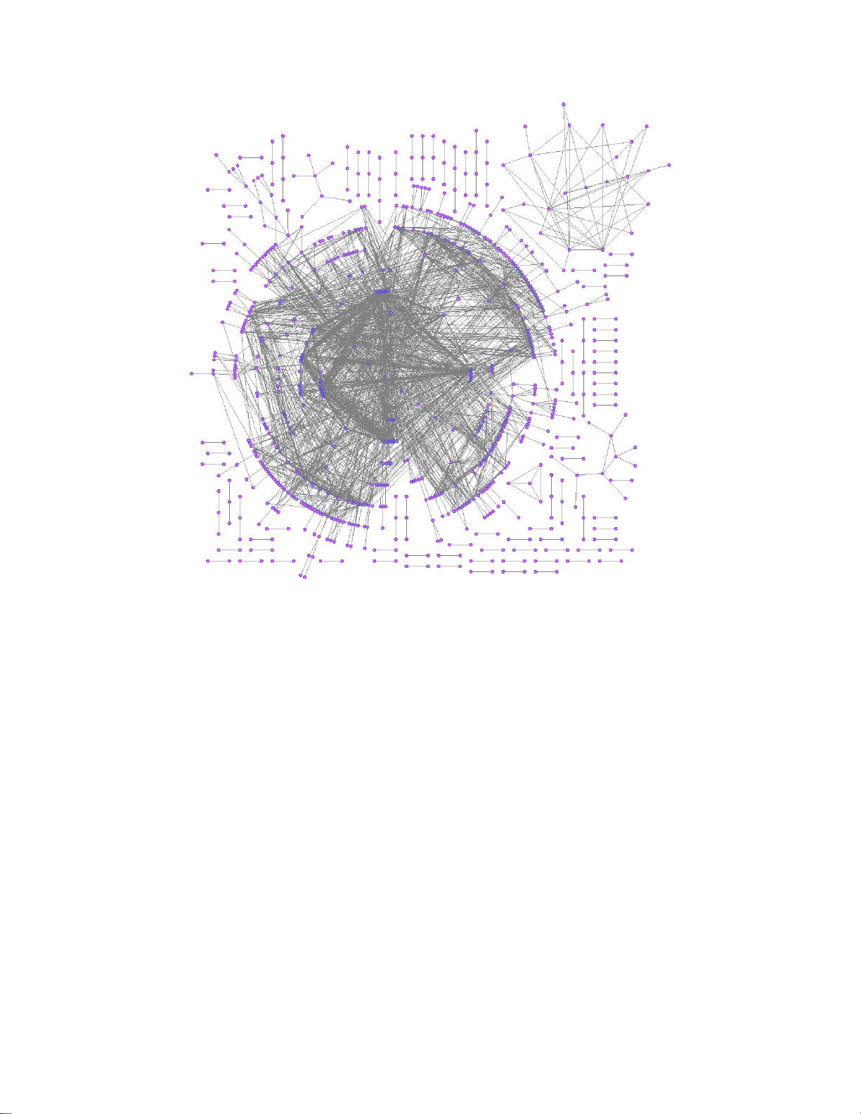
Large Scale Correlation Screening Alfred Hero Department of EECS, BME a nd St a tisti cs Universit y of Mic higan, Ann Ar b or, MI 48109 Bala Ra jarat nam Department of Statisti cs Stanfor d Universit y , Stanfor d, CA 9430 5 Octob er 22, 2018 Note that this arxiv v ersion is an updated v ersion of the tec hnical rep ort up- loaded on Arxiv on F ebruary 06, 2011. An earlier v ersion of this rep ort su bmitted for publication on Marc h 31, 2010 is also a v a ilable on request. Abstract This paper treats the problem of screening for v a riables with high correlations in high dimensional d ata in whic h there can b e many few er samples than v ariables. W e fo cus on thresh old-based correlation screening metho ds for three related applications: screening for v a riables with large correlatio ns within a single tr eatmen t (autocorre- lation screening); screening for v aria bles with large cross-correlations ov er t wo treat- men ts (cross-co rrelation screening); scree ning for v ariables that ha ve p ersistentl y large auto-correlat ions o ve r t w o treatmen ts (p ersistent-co rrelation screening). The no v elt y of correlation scr eenin g is that it ident iﬁes a sm aller num b er of variables wh ic h are h ighly correlated with others, as compared to iden tifying a num b er of correlation p ar ameters . Correlation s creening suﬀers from a p hase transition phenomenon: as the correlation threshold decreases the num b er of disco v eries increases abruptly . W e obtain asymptotic expressions for the mean num b er of d iscov eries and the phase transition th r esholds as a fun ction of the n umber of samples, the num b er of v ariables, and the join t s ample distribution. W e also show th at und er a w eak dep endency condition th e num b er of disco v eries is dominated by a P oisson r andom v ariable giving an asymptotic expr ession for th e false p ositiv e rate. The correlation screening approac h b ears tremen d ous divi- dends in terms of the type and strength of the asymp totic r esu lts that can b e obtained. It also o v ercomes some of th e m a jor h urd les faced by existing metho ds in the litera- ture as correlation scr eenin g is natur ally scalable to high dimension. Numerical results strongly v alidate the theory th at is presented in this pap er. W e illustrate the applica- tion of the correlation screenin g metho d ology on a large scale gene-expression dataset, rev ealing a few inﬂuential v ariables that exhibit a signiﬁcan t amoun t of correlation o ve r m ultiple tr eatmen ts. Keyw ords: High dimensional inference, V ariable selection, Phase tr ansition, Poisson limit, R´ en yi en trop y , Thr esholding, S parsit y , F alse disco very . 1 1 In tro d uction Consider the problem of screening for v ariables tha t ha v e signiﬁcant correlations in a large data set. Examples of suc h data sets are gene expression arra ys, m ultimedia databases, m ultiv ariate ﬁnancial time series , and traﬃc o v er the In ternet. Correlatio n screening can b e used t o discov er a small n um b er of v ariables that are highly corr elat ed or whose correlations ha v e distinct patterns, or motifs, that are no t lik ely to o ccur b y c hance. Indeed, ﬁltering out all but the highest sample correlations may b e the only practical w a y to examine dep en- dencies in massiv e da tasets where computational limitations prev ent the experimen ter from ev aluating all sample correlations. As an example, in m ulti- c hip gene expression data the n um b er o f pair wise correlations can b e in the billions. Thresholding the sample correlatio n matrix is a n attractiv e screening metho d due to its simplicit y . Ho w ev er, the threshold m ust b e c hosen with care due to the existence o f an abrupt phase tra nsition phenomenon controlling the n umber of disco v eries. When the correlation threshold falls b elo w a critical p oin t the n umber of disco v eries abruptly and rapidly increases, ev en when the v ariables a r e uncorrelated. This critical p oin t can b e close to one when the n um b er p of v a riables greatly exceeds the n umber n of samples. Therefore a p o orly selected correlation t hreshold ma y result in a n o v erwhelmingly lar g e nu m b er of discov eries. This pap er provides theory that predicts the lo cation of this critical p o in t as a function o f n , p , and the joint distribution of the v ariables. When the p o pula t io n cov aria nce matrix is o f large dimension and sparse the theory sp eciﬁes univ ersal thresholds that do not depend on the unkno wn m ultiv ariate sample densit y . W e distinguish b et wee n three t yp es of screening whic h arise in practical applications in- v olving a single t r eatmen t or a pair of treatmen ts. Each t yp e of screening seeks to disco v er v ariables with the prop erty that they are highly correlated with at least one other v ar iable. The ﬁrst application in v olv es screening for v ariables that are hig hly correlated with other v ariables in undergoing the same treatmen t. The second application is screening for v ariables in one treatmen t that are highly correlated with v aria bles undergoing a diﬀeren t treatmen t. 2 The third application is screening for v ariables with hig h within-treatmen t correlation that p ersists o v er a pair of treatmen ts. Precise deﬁnitions are giv en in Section 3. W e resp ec- tiv ely call these three applications auto-correlatio n scree ning, cross -correlation screening, and p ersisten t-correlation scree ning. In each of these problems the lo cation of the phase transition critical p o int is diﬀeren t. F or eac h of these three applications we index the correlation threshold ρ p b y the n um b er of v ariables p . W e giv e asymptotic conditions on t he sequenc e { ρ p } p that guarantee a ﬁnite and non- zero mean nu m b er of discov eries. These conditions, whic h dep end o n the num b er n of samples, can b e used to guide the selec tion of an appropriate correlation threshold in practical applications. Under these conditions we deriv e asymptotic express ions for the mean num b er of discov eries. Thes e expressions depend on a Bhattac haryy a measure [3] of a v erage pairwise dep endency of the p m ultiv ariate U-scores deﬁned on the ( n − 2 )-dimensional h yp ersphere. It is throug h this pairwise dep endency measure t ha t the p opulation co v ariance matrix inﬂuences the mean num b er of disco v eries. W e establish simple ac hiev able b ounds that giv e insigh t into factors that determine the mean num b er of disco v eries. These b o unds in v olv e R ´ eny i en tropy [18 ] and o t her information theoretic quan tities. F or example, we sho w that the mean disco v ery rate is prop ortional to the order 2 R ´ en yi en tropy of the av erage marginal densit y of asso ciated U-scores if and only if these scores are indep enden t iden tically distributed. Under this i.i.d. condition the mean n um b er of auto-correlatio n screening discov eries is minimized f o r the case of uniformly dis- tributed U- scores. This establishes a minimal pr o p ert y of the p -v ariate spherical distribution o v er the elliptical dia gonal disp ersion family . Using the expressions for the mean nu m b er of disco v eries we sp ecify the critical p oin t ρ c of the phase transition. As either p increases or n decreases ρ c approac hes one, making reliable screening imp ossible, and ρ c approac hes this limit with rate ro ughly equal to p − 1 /n . In partic- ular, f or auto-correlation screening, when n > 4 and p is large: ρ c = p 1 − c n ( p − 1) − 2 / ( n − 4) , where c n dep ends on the a foremen tioned Bhatta charyy a measure of a v erage pairwise depen- 3 dency of the U-scores and only dep ends w eakly on n . W e also establish that under a w eak dep endency assumption the n um b er of disco v eries is a symptotically dominated by a related P oisson random v ariable. In the case of auto- correlation and cross-correlation screening this P o isson v ariable is the n um b er of p ositiv e v ertex degrees in the associat ed sample correlation graph. In the case of p ersisten t- correlation screening the dominating P oisson v ariable is the correlation of the vertex degrees in the sample correlation gr aphs asso ciated with eac h treatmen t. The weak dependency condition on the av erage U-score pairwise distributions is satisﬁed for v ariables whose cov aria nce matrix is sparse or whose correlations ar e small. These dominance results specify an asymptotic expression for the false p ositiv e rate of disco v eries that can b e used to select the screening threshold to con trol the fa milywise dis- co v ery ra te. F amilywise disco v ery rate has b een widely used in v ar ia ble selection problems. The rate function in our derived P oisson limit sp eciﬁes the marg inal false disco v ery ra te asso- ciated with a part icular correlation threshold. While w e do not explore it in this pa p er, when suitably corrected fo r dep endency , the asso ciated p-v alues migh t also b e used to con trol the conditional false disco v ery ra te. F or a g iv en pair of v ariables and a giv en screening threshold, the bias-corrected normal appro ximation to the Fisher Z transformed sample correlations al- lo ws us to approx imate the minimum detectable cor r elat io n b etw een t he v a riables. W e giv e a n umerical example tha t provides exp erimen tal v alidation and illustrates the practical utilit y of our theoretical predictions f o r large but ﬁnite p and small n . W e then apply our metho d to corr elation screening of a large scale Aﬀymetrix gene micro-array dataset fo r analysis of a four treatmen t b everage in tak e exp erimen t [4]. The correlation screening problem treated here is not related to in v erse cov ariance and co v ariance selection problems studied b y man y authors (see [6, 13, 1 9, 9, 8, 17] to name just a few from an increasing literature). Unlik e these authors who are in terested in correlation or co v a riance matrix estimation with respect to a matrix error norm, here we are concerned with detection of a few v ar iables with large correlation co eﬃcien ts. Unlike previous w ork 4 in cov a riance selection w e prov ide precise phase transition thresholds that are applicable to large scale screening for correlation and persistence in single and mu ltiple treatmen ts. This pap er is related to tests o f signiﬁcance for co v ariance and correlation mat r ices [11, 7], but our fo cus is correlation screening instead of testing for diagonal co v ariance or for other structure. T ests of diagona l co v ariance structure are o f ten ba sed on the maxim um sample correlation co eﬃcien t, whic h has recen tly b een studied in the large p regime [12, 14, 15, 16, 21]. Unlik e the correlation screening results sho wn in this pap er, these studies often imp ose more stringen t (G a ussian) a ssumptions o n the joint distribution of the v ariables and do not consider the case of p ersisten t maximal correlation. On the other hand, our results could b e of practical v alue in b oth cov a riance selection and correlation tests of signiﬁcance, esp ecially when p is large. Correlation screening is an eﬀectiv e metho d for disco v ering a few highly correlated v ari- ables when there a re no resp onse v ariables in the dat a , i.e., it is an unsup ervised metho d. While our form ulation of correlation screening do es not sp eciﬁcally t a rget the sup ervised problem of v aria ble selection for regression, t he correlation screening framew ork can b e ap- plied to this setting. Speciﬁcally , the exp erimen ter would apply correlation screening to a sample of concatenated v ectors con ta ining b oth indep enden t v ar ia bles and resp onse v ari- ables. An y indep enden t v a riable discov eries that hav e high cross-correlation with a resp onse v ariable w ould b e excellen t candidates to include in the regression algorithm. The outline of the pap er is as follow s. In Section 2 the main assumptions are stated and the mathematical notatio n is giv en. In Section 3 the diﬀeren t kinds of correlation screening tests are deﬁned and the asymptotic theory is dev elop ed and discusse d. In section 4 the a symptotic theory is sp ecialized to the case of blo c k-sparse p o pulation co v ariance. In Section 5 n umerical results and experiments are presen t ed to illustrate the theory . Pro ofs of the principal results in the pap er are g iven in the App endix/Supplem en tal Section. W e also refer t he reader to a tec hnical r ep ort whic h contains more details o n the results in this pap er (see [10]). 5 2 Preliminaries In t his section w e set the notat io n and recall some classic al results on sample correlation. See Anderson [1], for example, f or more bac kground. Let X = [ X 1 , . . . , X p ] T b e a v ector of random v ariables with mean µ a nd p × p co v ariance matrix Σ . Deﬁne the correlation matrix Γ = D − 1 / 2 Σ ΣD − 1 / 2 Σ where D Σ = diag i ( Σ ii ) is the diagonal matrix of v a riances of comp onents of X . Assume that n samples of X are av ailable and arrange these samples in a n × p data m atrix X = [ X 1 , · · · , X p ] = [ X T (1) , · · · , X T ( n ) ] T , where X i = [ X 1 i , . . . , X ni ] T and X ( i ) = [ X i 1 , . . . , X ip ] denote the i -th column and row, resp ectiv ely , of X . Note that most of the results in this pap er hold when the rows of X are dep enden t. Deﬁne the sample mean of the i -th column X i = n − 1 P n j =1 X j i , the v ector of sample means X = [ X 1 , . . . , X p ], the p × p sample co v ariance mat r ix S = 1 n − 1 P n i =1 ( X ( i ) − X ) T ( X ( i ) − X ), a nd the p × p sample correlation matrix R = D − 1 / 2 S SD − 1 / 2 S , where D S = diag i ( S ii ) is the dia g onal matrix of comp onen t sample v ariances. Let the ij -th en try of the ensem ble co v ariance Γ b e denoted γ ij and the ij -th en try of the sample cov ar iance R b e r ij . The multiv a riate Z-scores Z i ∈ I R n are constructed b y standardizing the columns X i of X to ha v e sample mean equal to zero and sample v ar ia nce equal to one Z i = X i − X i 1 p S ii ( n − 1) , i = 1 , . . . , p, where 1 is a vec tor of o nes. Equiv alen tly , Z = [ Z 1 , . . . , Z p ] = ( n − 1) − 1 / 2 ( I − n − 1 11 T ) X D − 1 / 2 . The Z-scores lie on t he inters ection of the n − 1 dimensional h yp erplane { u ∈ I R n : 1 T u = 0 } and the n − 1 dimensional sphere { u ∈ I R n : k u k 2 = 1 } . The correlatio n matrix has the Z-score represen tation R = Z T Z . 6 An equiv alen t represen tation for the sample correlation matrix R uses what w e call the U-scores, U i ∈ I R n − 1 : R = U T U , (2.1) where U = [ U 1 , . . . , U p ] is ( n − 1) × p . The U- scores lie on the ( n − 2)- sphere S n − 2 in I R n − 1 and are constructed b y pro j ecting a w a y the comp onen ts of the X i ’s orthogonal to the n − 1 dimensional h yp erplane { u ∈ I R n : 1 T u = 0 } , i = 1 , . . . , p . Sp eciﬁcally , deﬁne the orthogo nal n × n mat r ix H = [ n − 1 / 2 1 , H 2: n ]. The matrix H 2: n can b e obtained b y Gramm-Sc hmidt orthog o nalization and satisﬁes the prop erties 1 T H 2: n = [0 , . . . , 0] , H 2: n T H 2: n = I n − 1 . The U-score matrix U = [ U 1 , . . . , U p ] is obtained from Z by the f o llo wing relation U = H 2: n T Z . (2.2) F urthermore, the sample corr elat io n b etw een X i and X j can b e computed using the inner pro duct or the Euclidean distance b et w een asso ciated U-scores r ij = U T i U j = 1 − k U i − U j k 2 2 2 . (2.3) As the U- score is an ( n − 1)-elemen t v ector it is a more compact represen tation of the sample correlation than the n - elemen t Z-score ve ctor. More imp o rtan tly , the U-score live s in a geometry , the ( n − 2)- sphere o f co-dimension 1 sho wn in Fig. 1, that is simpler than that of the standard Z-score. Elliptically contoured distributions The results in this pap er hold for a wide class of sample distributions that include ligh t 7 and hea vy t a iled distributions suc h as the multiv ariate normal and m ultiv ariate student-t, resp ectiv ely . A random v ector X is said t o follow an elliptical distribution with lo cation parameter µ and disp ersion matrix parameter Σ if its density has the form f X ( x ) = | Σ | − 1 / 2 g  ( x − µ ) T Σ − 1 ( x − µ )  , (2.4) where g ( u ) is a non-negativ e monoto nic function. When Σ is a diagonal matrix the elliptical distribution is called d i a gonal el li p tic al . It is w ell kno wn that when the ro ws of the data matrix X are i.i.d. and follow a diagonal elliptical distribution the U-scores are uniformly distributed on S n − 2 , see fo r example [Sec. 2.7][1]. In the case of non- diagonal Σ the distri- bution of t he U-scores ov er the sphere S n − 2 will generally b e far from unifor m (Fig. 1). The U-score represen tations ( 2 .1) and (2.3) of the sample correlation will b e a k ey ingredien t for deriving the asymptotic results in this pap er. In v ok ed in the sequel will b e t he f o llo wing sparsit y condition on the disp ersion mat rix. The matrix Σ = (( σ ij )) i,j is said to b e row-sparse of degree k if ev ery row has f ew er than k + 1 non- zero en tries. F orma lly , { i : |{ j : σ ij 6 = 0 }| > k } = ∅ , (2.5) where ∅ is the empty set. When the matrix is row -sparse of degree q and there exists a p erm utation that blo c k diag onalizes Σ then the matrix satisﬁes the q -sparse condition of Sec. 4. Relev an t deﬁnitions: The asymptotic expressions f o r the mean n um b er of disco v eries in the next section will b e a function of sev eral quantities in t r o duced b elow . Spherical Cap Probabilit y 8 Figure 1: The U-scores asso ciated with n = 4 realizations of 500 v ariables are n − 1-elemen t v ectors that lie on the unit n − 2 dimensional sphere S n − 2 . Show n are U-scores fo r a m ultiv ari- ate normal sample. A t left: for diagona l cov a r ia nce matrix the 500 U-scores ar e uniformly distributed ov er S n − 2 . At rig ht: for a non-diago nal co v ariance the U-scores are fa r from uniformly distributed o n S n − 2 . Pairs of U-scores that are close to each other, as measured b y Euclidean distance, ha v e high asso ciated sample correlations. Deﬁne P 0 = P 0 ( ρ, n ) = a n Z 1 ρ  1 − u 2  n − 4 2 du, (2.6) where a n is a n = 2Γ(( n − 1) / 2) √ π Γ(( n − 2 ) / 2) . (2.7) The quan tit y P 0 / 2 is equal t o the pro p ortional area of the spheric al c a p of ra dius r = p 2(1 − ρ ) on S n − 2 . It is the pro babilit y that a uniformly distributed p oint U on the sphere lies in pair of h yp erspherical cones symmetric ab o ut the o r igin. This pr o babilit y expression w as deriv ed in the con text of the spherical normal distribution by R ub en [20, Eq. 4.1]. 1 A p o w er series expansion of the in tegral in (2.6) yields the relation, accurate as ρ 2 approac hes 1 The integral in [2 0, Eq. 4.1] is obtained from the integral in (2.6) by making change of v ariable θ = arccos( u ). 9 1: P 0 ( ρ, n ) = ( n − 2 ) − 1 a n (1 − ρ 2 ) ( n − 2) / 2 (1 + O (1 − ρ 2 )) . (2.8) Relev an t en trop y and divergence quan tities F or a give n densit y f on S n − 2 deﬁne the following en trop y-related functional, whic h satisﬁes the indicated inequalit y H 2 ( f ) = | S n − 2 | Z S n − 2 f 2 ( u ) d u ≥ 1 . (2.9) Equalit y is attained in the inequality (2.9) if and only if ( iﬀ ) f is the uniform densit y: f ( u ) = | S n − 2 | − 1 . H 2 ( f ) is a monotonic transformation of the R ´ eny i entrop y of f of o rder 2: − log ( | S n − 2 | − 1 H 2 ( f )) . F or a joint densit y f U , V on S n − 2 × S n − 2 with marginals f U and f V deﬁne J ( f U , V ) = | S n − 2 | Z S n − 2 f U , V ( u , u ) d u . (2.10) It will b e shown that J ( f U , V ) inﬂuences the mean n um b er of disco v eries. Therefore, sev eral in tuitiv e interpre tations are give n b elo w that will b e of use in the sequel. First, J ( f U , V ) is a measure of dep endence b et wee n U , V . Sp eciﬁcally , it is equal to the Bhattac haryy a a ﬃnit y b et w een f V ( w ) f U ( w ) and the pro duct f U | V ( w | w ) f V | U ( w | w ): J ( f U , V ) = | S n − 2 | Z q f U | V ( w | w ) f V | U ( w | w ) p f U ( w ) f V ( w ) d w . (2.11) This is maximized when U , V are statistically indep enden t. Second, the following asymptotic represen tatio n follows f r om (A.16): J ( 1 2 f U , V + 1 2 f U , − V ) = lim ρ → 1 P  min {k U − V k 2 , k U + V k 2 } ≤ p 2(1 − ρ )  P 0 ( ρ, n ) . 10 The limit is equal to one when U and V are independen t a nd uniformly distributed on S n − 2 . Th us J ( f U , V ) − 1 is a measure of the deviation of the joint density f rom uniform f U , V ( u , v ) = | S n − 2 | 2 . This measure can either b e p ositiv e, e.g., when U and V are highly correlated or anti-correlated, or negativ e, e.g., when f U , V ( u , v ) has nearly zero mass in the vicinit y o f the diagonal u − v = 0 and an tidiagonal u + v = 0 regions. Finally , the f o llo wing simple inequalities giv e further insigh t in to J ( f U , V ): J ( f U , V ) ≤ | S n − 2 |  Z f U | V ( w | w ) f V | U ( w | w ) d w  1 / 2  Z f U ( w ) f V ( w ) d w  1 / 2 ≤ H 1 / 4 2 ( f U | V ) H 1 / 4 2 ( f V | U ) H 1 / 4 2 ( f U ) H 1 / 4 2 ( f V ) , (2.12) where equality in the ﬁrst inequalit y and the second inequality o ccur iﬀ f U , V ( u , u ) = f U ( u ) f V ( u ) and f U ( u ) = f V ( u ), resp ectiv ely . Hence J ( f U , V ) is maximized when U and V ar e indep endent. In t he o t her direction, when restricted to the case of indep enden t U and V , J ( f U , V ) = H 1 / 2 2 ( f U ) H 1 / 2 2 ( f V ) is minimized when U and V are uniform ov er S n − 2 . 3 Correlatio n screeni ng Consider a n exp erimen t to compare p v ariables under treatmen ts a and b , called X a and X b . The n um b er n of sample realizations may be diﬀeren t in the tw o exp erimen ts but the num b er and identit y of the p v a r ia bles ar e the same. Thes e exp erimen ts pro duce tw o data matrices: X a and X b , whic h are n a × p and n b × p matrices, resp ectiv ely . F rom these data matrices extract the U-score matrices U a and U b . Then, using the represen tation (2.1) , w e construct R a = [ U a ] T U a and R b = [ U b ] T U b , and call them sample auto-correlation matrices. When n a = n b w e can a lso construct the sample cross-correlation mat rix R ab = [ U a ] T U b . W e are primarily interes ted in the case n a , n b ≪ p so that the auto- cor r elation a nd cross-correlation matrices will b e rank deﬁcien t. L et the ij -th elemen t of eac h of these matr ices b e denoted as r a ij , r b ij , and r ab ij , resp ectiv ely . W e distinguish b et w een three t yp es o f correlation screening. W e use the terms auto- 11 correlation and cross-correlation in analogy to auto-correlation and cross-correlation func- tions in time series analysis. Auto-correlation screening : The ob jectiv e is to screen the p v ariables for those whose maximal magnitude correlation exceeds a give n threshold ρ a . Sp eciﬁcally , for i, j = 1 , . . . , p , the i -th v ariable passes the screen if: max j 6 = i | r a ij | > ρ a . (3.1) Cross-correlation screening : The ob jectiv e is to screen the p v a r iables for those whose maximal magnitude cross-correlation exceeds a give n threshold ρ ab . Sp eciﬁcally , for i, j = 1 , . . . , p , the i -th v aria ble passes the screen if: max j 6 = i | r ab ij | > ρ ab . (3.2) P ersisten t auto-correlation screening : The ob jectiv e is to screen the p v ariables for those whose maximal magnitude a ut o -correlation in b oth t r eat ments exceeds giv en thresholds ρ a and ρ b , resp ectiv ely . Sp eciﬁcally , for i = 1 , . . . , p , the i -th v ariable passes the screen if: max j 6 = i | r a ij | > ρ a and max j 6 = i | r b ij | > ρ b . (3.3) F or eac h of the a b o v e three tests a disco v ery is declared if an index i passes the screen and w e denote b y N a , N ab , and N a ∧ b , r esp ectiv ely , the tota l num b er of discov eries. F or large p , these t hree tests display similar phase t r a nsition phenomena. F o r example, w e illustrate in Fig. 2 how the num b er N a of false auto-correlation disco v eries exp eriences a sharp increase as the threshold ρ a is reduced b ey ond a certain critical v alue ρ c . This critical v alue depends on the num b er p of v ariables, the n um b er n = n a of samples, and the j o in t distribution of the p v a r ia bles. The b eha vior gets w orse a s n decreases relative to p , eve n tually o verwh elming the test with false disco v eries for all but a nar r ow range of thresholds ρ close to 1. 12 Figure 2 : Eﬀect of n umber o f samples n on the disco v eries for a m ultiv ariate normal sample where all but tw o of the p = 500 v ariables are m utually correlated as n decreases o v er the range 50 , 25 , 10. These t w o v ariables ha v e a correlation co eﬃcien t equal to ρ 1 = 0 . 8. Show n are histograms of the p ( p − 1) / 2 distinct sample correlation co eﬃcien ts in the correlation matrix R excluding the diago na l co eﬃcien ts. The arro ws p oin t to the lo cations of the p ositiv e and negativ e correlation thresholds of an auto-correlation screening test that w ould detect the v a r iables ha ving a t least 0 . 8 correlation with probability not exce eding 0 . 5. An increasing n um b er of other sample correlations exceed t his threshold as n decreases: these false disco v eries are o v erwhelming for small n . In the next three subsections w e dev elop theory to predict this phase transition b ehavior in terms of the mean num b er of disco v eries. 3.1 Disco v eries in auto-correlation screening Here w e giv e results for the mean num b er of disco v eries E [ N a ] when screening for t hr eshold- exceeding correlations b etw een columns of a single data matrix X a . F or con v enience here we suppress “ a ” sup erscripts a nd subscripts. W e recall the quantities γ p = max 1 ≤ k < p { a k n M k | 1 } , η p = 2 a 2 n ˙ M 1 | 1 (3.4) where a n = | S n − 2 | , M k | 1 is deﬁned in (A.2) and ˙ M 1 | 1 is deﬁned in (A.4). These quan tities are unifor mly b ounded o v er p when the joint densit y f U 1 ,..., U p of the U-scores is smoo th and strictly b ounded b et w een (0 , ∞ ) . F or example if the j o in t densit y of the Z -scores is a ﬁnite 13 mixture of v on Mises-Fisher densities on the sphere S n − 2 with strictly b ounded concen tration parameters, then γ p and η p are uniformly b ounded. Prop osition 1. L et the n × p data matrix X have ass o ciate d U-sc or e s U and ass ume that n > 2 . Assume that γ p and η p ar e uniforml y b ounde d. L et the se quenc e { ρ p } p of c orr elation thr esholds b e such that ρ p → 1 and p ( p − 1)  1 − ρ 2 p  ( n − 2) / 2 → e n for som e ﬁnite c onstant e n . Then the me an numb er of disc ove ri e s gene r ate d fr om the auto-c orr elation scr e en (3.1) satisﬁes:   E [ N ] − κ n J ( f U • , U ∗−• )   ≤ O ( p − 1 ) + O ( p 1 − ρ p ) , (3.5) wher e κ n = a n e n / ( n − 2) and f U • , U ∗−• ( u , v ) = 1 p p X i =1 1 p − 1 p X j 6 = i  1 2 f U i , U j ( u , v ) + 1 2 f U i , U j ( u , − v )  , (3.6) is the aver age of the p airwise U-sc or e density. Assume in addi tion that the jo i n t density of the U-sc or es satisﬁe s the we ak dep ende n cy c ondition: for some k = o ( p ) the aver age de p endency c o eﬃ c ient k ∆ p,k k 1 (A.13) c on ver ges to zer o . Then P ( N > 0) → 1 − exp( − Λ / 2) whe r e Λ is the limiting value of E [ N ] sp e ciﬁe d by (3.5). In the pro of of Prop. 1 we establish the stated limit on P ( N > 0) b y showing that N is dominated by the num b er N e of edges in the correlation gr a ph and that N e con v erges to a P oisson random v ariable N ∗ with rate Λ / 2 a s p → ∞ . The rate of conv ergence of P ( N > 0) to the stated limit is o f order max { ( k /p ) 2 , k ∆ p,k k 1 } . In terms of the limiting v alue (3.5 ) of E [ N ] the case where the columns of X ha v e spherically contoured distribution is of sp ecial interest. In this case the U- scores are i.i.d. uniformly distributed and J ( f U • , U ∗−• ) = 1. Prop. 1 asserts the w eak er necessary and suﬃcien t condition: J ( f U • , U ∗−• ) = 1 if and only if the a v eraged pairwise U- score densit y (3.6) is i.i.d. unifo r m o v er S n − 2 × S n − 2 . W e dev elop this further in the next paragraph. 14 n 550 500 450 150 100 50 10 8 6 ρ c 0.188 0.197 0.207 0.344 0.413 0.559 0.961 0.988 0.9997 T able 1 : V alues of the critical threshold ρ c where phase transition o ccurs in Fig. 3. These v alues w ere determined using asymptotic approximation (3.11). First observ e that the marg inal densities, obtained b y integrating f U • , U ∗−• ( u , v ) o v er v and u , are iden tical a nd equal to the a v erage U-score densit y f U ∗ ( u ) = 1 p p X i =1  1 2 f U i ( u ) + 1 2 f U i ( − u )  . (3.7) Therefore inequalit y (2.1 2) implies that J ( f U • , U ∗−• ) ≤ H 1 / 4 2 ( f U | V ) H 1 / 4 2 ( f V | U ) H 1 / 2 2 ( f U ∗ ) , (3.8) with equalit y iﬀ f U • , U ∗−• ( u , u ) = ( f U ∗ ( u )) 2 , whic h satisﬁed when the U-scores are indep en- den t. Second observ e that the extremal prop erty (2.9) of H 2 ( f ) implies t ha t, a mong all suc h i.i.d. U-score distributions, E [ N ] will b e smallest when the marginal f U ∗ is uniform, whic h is satisﬁed when the U-scores are unifo r m on S n − 2 . In the case that f U ∗ , U ∗−• ( u , u ) = | S n − 2 | − 2 , (3.5) implies the asymptotic approximation for ﬁnite p and ρ < 1: E [ N ] ≈ κ n ≈ p ( p − 1) P 0 ( ρ, n ) , (3.9) since p ( p − 1) P 0 ( ρ p , n ) → κ n as p → ∞ . This case ho lds, for example, when the row s of X are i.i.d. with diagonal elliptical distribution. In this case the U-scores are i.i.d. uniform and the mean nu m b er of disco v eries has the exact expression E [ N ] = p (1 − (1 − P 0 ( ρ, n )) p − 1 ) . (3.10) 15 Figure 3 : Normalized mean num b er of discov eries E [ N ] /p for the case that the ro ws of the data matrix are normal with diagona l co v ariance. Nine curv es a re plot ted as a function of the screening threshold ρ for p = 5 00 and nine v alues of n . The v alues n = 550 , 50 0 , 450 , 150 , 1 00 , 50 , 10 , 8 , 6 index the curves from left to righ t. In Fig. 3 w e plot the exact express ion (3.10 ) for the normalized mean n um b er of dis- co v eries as a function o f ρ and n for p = 500. Eac h curve , decreasing monotonically as ρ increases, is a plot of E [ N ] /p for g iv en n . Since the true cov ariance matrix is diago nal all disco v eries are false disco v eries. W e mak e sev eral observ ations: • The curv es in Fig. 3 cluster into thr ee groups. F rom left to righ t : n ∈ { 550 , 50 0 , 450 } , n ∈ { 150 , 100 , 50 } and n ∈ { 10 , 8 , 6 } . The eﬀect on the curv es of v arying n is more pronounced for small n tha n for lar g er n . • The curv es illustrate a phase tr a nsition phenomenon in the mean n um b er o f false p ositiv es a s a function of the threshold ρ . F or given n there is a critical p oint ρ c suc h that as ρ approac hes ρ c from ab o v e the mean n um b er of false p ositiv es is small and increases v ery slo wly . As ρ contin uous to decrease in the vicinit y of ρ c the mean n um b er of false p ositiv es increases rapidly to p . • The rapidit y of the phase transition v aries as a function o f n and is related t o the slop e of the curv e near its inﬂection p oint. The most rapid phase transitions o ccur when n is v ery large or very small. The phase transition threshold v alue ρ c can b e predicted b y the knee o f t he curv e in Fig. 16 3, deﬁned as the maxim um v alue ρ a t whic h the slop e of the curv e equals minus one. This c hoice of critical slop e is common in the ph ysics literature. One could c ho ose a diﬀeren t critical slop e v alue to deﬁne ρ c but this w ould only hav e a minor eﬀect (a change in the quan tit y c n in (3.10) by a constan t scale factor ). The slop e o f the large p approximation (3.5) to E [ N ] is dE [ N ] /dρ = − p ( p − 1)(1 − ρ 2 ) ( n − 4) / 2 a n J ( f U • , U ∗−• ) , where a n is giv en in (2.7). Deﬁne the critical v alue as ρ c = max { ρ : p − 1 dE [ N ] /dρ = − 1 } . F or n > 4 this is maximization can b e solv ed to g iv e the expression ρ c = q 1 − c n ( p − 1) − 2 / ( n − 4) , (3.11) where c n =  a n J ( f U • , U ∗−• )  − 2 / ( n − 4) . The accuracy of ρ c deﬁned in (3.11) can b e appreciated b y comparing the predicted ρ c in T able 1 to the t ransition p oints of the asso ciated curv es in Fig. 3. 3.2 Disco v eries in cross-correlation screening Next w e turn to screening for threshold-exceeding cross-correlations b etw een columns of tw o data matrices X a and X b . The theory in the previous section could b e directly used by applying Prop. 1 to the concatenated n × 2 p data matrix X =  X a X b  . Ho w ev er, the conv ergence rates and pha se tr ansition thresholds w ould b e signiﬁcan t ly w orse than b efore due to the inﬂation of the n um b er of v ariables from p to 2 p . F ur t hermore, if we thresholded the en tire 2 p × 2 p sample correlatio n matrix X T X we w ould exp ect that in most practical problems the aut o -correlation disco v eries in the diagonal blo c ks would dominate 17 the cross-correlation disco v eries in the oﬀ- diagonal blo c ks. The follo wing result is useful when one is only intere sted in the cross-correlation disco v eries. Deﬁne γ ab p and η ab p similarly t o (3 .4) except that M k | 1 and ˙ M 1 | 1 are replaced by M ab k | 1 and ˙ M ab 1 | 1 as deﬁned in (A.5) and (A.6 ). Prop osition 2. L et the n × p data m a tric es X a and X b have asso cia te d U-sc or es U a and U b and a s s ume that n > 2 . Assume that γ ab p and η ab p ar e uniformly b ounde d . L et the se quenc e { ρ p } p of cr oss-c orr e lation thr esholds b e such that ρ p → 1 an d p 2  1 − ρ 2 p  ( n − 2) / 2 → e n for some ﬁnite c o n stant e n . Then the me an numb er of disc overies gener ate d fr om the c r oss-c orr elation scr e e n (3. 2 ) satisﬁe s:   E [ N ab ] − κ n J ( f U a ∗ , U b • )   ≤ O ( p − 1 ) + O ( p 1 − ρ p ) , (3.12) wher e κ n = a n e n / ( n − 2) and f U a ∗ , U b • = 1 p p X i =1 1 p p X j =1  1 2 f U a i , U b j ( u , v ) + 1 2 f U a i , U b j ( u , − v )  . (3.13) Assume in addition that the joint de n sity of the U-sc or es satisﬁes the we ak cr oss-dep endency c ondition: for some k = o ( p ) the a ver age dep enden cy c o eﬃcient k ∆ ab p,k k 1 (A.13) c onver ges to zer o. Then P ( N ab > 0) → 1 − exp( − Λ) wher e Λ is the limiting value of E [ N ab ] sp e ciﬁe d by (3.12). The critical phase tra nsition threshold for the case of cross-correlation screening can b e deriv ed in a similar manner to the previously considered case of auto- correlation screening. The critical threshold is give n b y ρ c = q 1 − c ab n p − 2 / ( n − 4) , (3.14) where c ab n =  a n J ( f U a • , U b • )  − 2 / ( n − 4) and a n is giv en in (2 .7 ). 18 3.3 Disco v eries in p ersisten t-correlation screening Finally we treat screening for v ariables whose a uto-correlation exceeds a threshold in b o th of tw o treatments a and b . Recall that in this problem there are tw o correlation thresholds ρ a and ρ b that are resp ectiv ely applied to the p × p sample corr elat io n matrices deriv ed from the indep endent data matrices X a and X b . As discussed below, Prop. 1 could b e directly applied to this problem but it w ould result in a n unin teresting degenerate limit. A more in teresting result is the follow ing. Prop osition 3. L et the n a × p data matrix X a and the n b × p data matrix X b b e statistic al ly indep end e nt and assume that the a s s o ciate d U-sc or e s fr om e ach tr e atment satisfy the same c onditions assume d for in Pr op. 1. L et the se quenc es { ρ a p } p and { ρ b p } p b e such that ρ a p → 1 and ρ b p → 1 wh i l e p 1 / 2 ( p − 1)  1 − ( ρ a p ) 2  ( n a − 2) / 2 → e n a and p 1 / 2 ( p − 1)  1 − ( ρ b p ) 2  ( n b − 2) / 2 → e n b for som e ﬁnite c onstants e n a , e n b . Then the me an numb er of disc overies N a ∧ b gener ate d by the p ersistent-c orr elation scr e en ( 3.3) s a tisﬁes (3.15)      E [ N a ∧ b ] − κ a ∧ b n 1 p p X i =1 J ( f U a i , U a ∗− i ) J ( f U b i , U b ∗− i )      ≤ O  max { ( k /p ) 3 , ( k /p ) p − 1 / 2 , p − 1 , k ∆ a p,k k 1 , k ∆ b p,k k 1 }  , wher e κ a ∧ b n = e n a e n b a n a a n b ( n a − 2) − 1 ( n b − 2) − 1 and, for U ∈ { U a , U b } , f U i , U ∗− i is the le ave- one-out aver ag e of the U-sc or e p airwise densities: f U i , U ∗− i ( u , v ) = 1 p − 1 p X j 6 = i  1 2 f U i , U j ( u , v ) + 1 2 f U i , U j ( u , − v )  . (3.16) Assume in addition that the U-sc or e densities asso ciate d with X a and X b e ach s a tisfy the we ak de p endency c on dition state d in Pr op. 1. T hen P ( N a ∧ b > 0) → 1 − exp( − Λ) wher e Λ is the limiting value of E [ N ] sp e ciﬁe d in (3. 1 5). In Prop. 3 the a ssumed r ates of con v ergence o f ρ a p , ρ b p are slow er (not e the diﬀeren t factor p 1 / 2 ) than t he ra tes assumed in Prop. 1 and 2. A slo w er rate is required since p ersisten t 19 correlation disco v eries are rar er t ha n auto-correlation disco v eries. In particular, when the correlation thresholds satisfy the hypotheses of Prop. 3 the individual p er-treatmen t means E [ N a ] and E [ N b ] do not con ve rge. Ho w ev er, it can b e sho wn that p − 1 / 2 E [ N a ] and p − 1 / 2 E [ N b ] do con verge (see Corollary 1 in App endix/Supplemen tal Section). Conv ersely , if the indi- vidual p er-treat ment means conv erge to ﬁnite v alues then the mean num b er of p ersisten t disco v eries E [ N a ∧ b ] con v erges to zero, resulting in an uninteres ting limit. Assume that one or the other of the factors in the summand of (3.15) do not dep end on i : J ( f U a i , U a ∗− i ) = J ( f U a • , U a ∗−• ) , or J ( f U b i , U b ∗− i ) = J ( f U b • , U b ∗−• ) . (3.17) When (3.17) ho lds w e sa y that the pairwise dep endencies are inc oher ent across treatmen ts a and b . A suﬃcien t condition fo r incoherence is pairwise independent U- scores with iden tical marginal densities f a U i = f a U j and f b U i = f b U j . In the incoherent case the limit (3.15) tak es on a simpler intuitiv e fo rm 1 p p X i =1 J ( f U a i , U a ∗− i ) J ( f U b i , U b ∗− i ) = J ( f U a • , U a ∗−• ) J ( f U b • , U b ∗−• ) . Deﬁne κ n a = p 1 / 2 e n a a n a / ( n a − 2 ) and κ n b = p 1 / 2 e n b a n b / ( n b − 2 ) . Then, in view of the limit (3.5) of Prop. 1, under the condition (3.17 ) the limit in (3.15) giv es the large p approximation E [ N a ∧ b ] ≈ E [ N a ] E [ N b ] p . (3.18) The right side of (3 .18) is equal to the rig h t side of (3 .15) when the pairwise dep endencies are incoheren t across treatments a and b . Relation (3 .18) is a w ell kno wn asymptotic relation for the num b er of mat ches in t w o indep enden t Bernoulli sequences o f length p . In this case N a ∧ b is the num b er of successes common to the pair of sequences and N a , N b are the num b er of successes in each sequence; 20 a result easily established using for large p Stirling approximations and assuming small probabilities of success. It is in t eresting that in p ersistenc y screening it is suﬃcien t that only one of the tw o treatments pro duce iden tically distributed U-scores for (3.1 8 ) to hold. W e next turn t o the problem of selecting the thresholds ρ a and ρ a . These thresholds aﬀect the asymptotic mean num b er of disco ve ries (3 .1 5) only through the limits e n a and e n b deﬁned in Prop. 3 When relation (3.18) holds, it can b e sho wn that if we ﬁx the normalized a v erage rate of p er-treatmen t disco v eries ( E [ N a ] + E [ N b ]) p − 1 / 2 / 2, E [ N ab ] is maximized when the thresholds ρ a and ρ b are chose n to ma ke E [ N a ] = E [ N b ]. These o ptimal thresholds a re related b y 1 − ρ 2 a = (1 − ρ 2 b ) n a − 2 n b − 2 ( n b − 2)a n a J ( f U a • , U a ∗−• ) ( n a − 2)a n b J ( f U b • , U b ∗−• ) ! 2 / ( n a − 2) . A general closed form expression for the critical phase t r a nsition threshold for p ersisten t- correlation screening has no t b een found. Ho we v er, for the sp ecial case of pairwise i.i.d. U-scores and equal num b er n = n a = n b of samples, the following express ion for the critical threshold holds ρ c = q 1 − c a ∧ b n ( p − 1) − 2 / ( n − 4) , (3.19) where c a ∧ b n =  a n  H 2 ( f U a ∗ ) H 2 ( f U b ∗ )  1 / 2  − 2 / ( n − 4) and a n is giv en in (2.7). Prop 3 generalizes to more than tw o treatmen ts. Ass ume there a re m diﬀeren t indep en- den t treatmen ts t 1 , . . . , t m then t he correlation thresholds ρ t j p should b e selected suc h that they conv erge to one and p 1 /m ( p − 1)  1 − ( ρ t j p ) 2  ( n t j − 2) / 2 con v erges to a ﬁnite constan t, sa y e n j , j = 1 , . . . , m . In this case o ne obtains the same ty p e of limit of the false p ositiv e rate as in Prop. 3 under similar conditions of w eak dep endence of the v ariables within each treatmen t. The mean n um b er of disco v eries will con v erge to lim p →∞ E [ N t 1 ∧···∧ t m ] = κ n lim p →∞ p − 1 p X i =1 m Y j =1 J ( f U t j i , U t j ∗− i ) (3.20) 21 where κ n = Q m j =1  a n j e n j n j − 2  . If min { n j } > 2( m + 1) and ˙ M 1 | 1 (deﬁned in (A.4)) is b ounded, the ra te of con v ergence in (3.20) will b e dominated b y the treatmen t with the fewe st samples and it will b e of order O  p − 2 / ( n − 2)  where n = min j { n j } . Otherwise the rat e of conv ergence will b e O ( p − 1 /m ). When the factor s in the summand of the limit (3 .20) do not dep end o n i a relation analogo us to ( 3 .18) holds: E [ N t 1 ∧···∧ t m ] ≈ ( E [ N t 1 ] · · · E [ N t m ]) /p m − 1 . 4 Correlatio n screeni ng wi t h sparse dep e n dency In this section w e sp ecialize to the class of q - sparse p × p co v aria nces, deﬁned as ro w-sparse co v ariance matrices of degree q that can b e reduced to a single q × q blo c k of correlated v ariables using row -colum p erm uta t ions. Under t his q -sparse condition, t o o r der O  ( q /p ) 2  the limits stated in Prop ositions 1-3 do not dep end on the unkno wn join t sample distribution. Therefore, these prop ositions can b e used to determine unive rsal screen ing thresholds tha t appro ximately con trol an y desired lev el of false p o sitive rate. W e treat each of t he three correlation screening pro cedures separately . 4.1 Sparse auto-correlati on screening Let the ro ws of X be i.i.d. Under the assumption t ha t the columns of X hav e q -sparse co v ariance, the U-scores { U a i } p i =1 are i.i.d. uniform except fo r a num b er of q ≤ p mu tu- ally dep enden t U-scores { e U a i } q i =1 that are indep enden t of the rest. The mean n umber of disco v eries in Prop. 1 b ecomes, to order at most O  max  p − 1 , p − 2 / ( n − 2)  , E [ N a ] = κ a n  1 + q ( q − 1) p ( p − 1)  J ( f e U a • , e U a ∗−• ) − 1   , where f e U a • , e U a ∗−• is the a v erage o v er the joint distributions o f distinct and m utually dep enden t U-scores. Therefore, t o or der at most O  max  ( q /p ) 2 , p − 1 , p − 2 / ( n − 2)  the mean n um b er of disco v eries is equal to κ a n . 22 4.2 Sparse cross-correlation screening Let the rows of X b e i.i.d. Assume tha t the cross correlation mat r ix is blo ck -sparse in the sense that there exists a column p erm uta t io n that puts the cross-correlatio n matrix in to a form having most entries zero except for a small q a × q b non-zero oﬀ dia g onal blo c k. Then the mean n umber of disco veries in Prop. 2 b ecomes, to order at most O  max  p − 1 , p − 2 / ( n − 2)  , E [ N ab ] = κ ab n  1 + q a q b p 2  J ( f e U a • , e U b • ) − 1   . Therefore, with q = max { q a , q b } , to order O  max  ( q /p ) 2 , p − 1 , p − 2 / ( n − 2)  the mean num b er of disco v eries is equal to κ ab n . 4.3 Sparse p ersisten t-correlation screening Let the row s of X b e i.i.d. Assume that under treatmen t a all v ariables are m utually uncorre- lated except for a those v ar ia bles with indices in the set Q a . Lik ewise deﬁne the index set Q b of v aria bles having non-zero correlatio n under treatment b . The mean n umber of disco v eries in Prop. 3 b ecomes, to order O  max  p − 1 / 2 , p − 2 / ( n − 2)  , E [ N a ∧ b ] /κ a ∧ b n = 1 +  | Q b − Q a | p   | Q b | − 1 p − 1  ( ˜ J b − 1) +  | Q a − Q b | p   | Q a | − 1 p − 1  ( ˜ J a − 1) +  | Q a ∩ Q b | p   | Q a | − 1 p − 1  ( ˜ J a − 1) +  | Q a ∩ Q b | p   | Q b | − 1 p − 1  ( ˜ J b − 1) +  | Q a ∩ Q b | p   | Q a | − 1 p − 1   | Q b | − 1 p − 1  ( ˜ J a − 1)( ˜ J b − 1) , where ˜ J a = J ( f e U a • , e U a ∗−• ) a nd similarly for ˜ J b . In particular, to o rder O  max  p − 1 / 2 , p − 2 / ( n − 2)  , if there is a q -sparse cov ariance under eac h treatment a nd there are common p ersisten t cor- relations among the q v ariables the E [ N a ∧ b ] = κ a ∧ b n  1 + O  q ( q − 1) p ( p − 1)  , 23 while if only one of the treatments , sa y treatment a , pro duces q - sparse co v ariance E [ N a ∧ b ] = κ a ∧ b n ˜ J b  1 + O  q ( q − 1) p ( p − 1)  . In pa rticular, in the latter case to order O  max  ( q /p ) 2 , p − 1 / 2 , p − 2 / ( n − 2)  the simple pro duct represen tatio n (3.18 ) holds. 5 Numerical exp erimen ts T o illustrate t he practical utility of the theory dev elop ed in the previous sections we presen t t w o n umerical studies. First sim ulations were p erfor med that sho w our false p ositiv e rat e appro ximations give accurate ﬁnite p appro ximations to empirically determined error rates in a sparse example. Second, these a ppro ximations ar e used to p erform correlation screening on experimental gene expression microar ra y data. 5.1 Sim ulation results W e used the asymptotic theory to specify suitable correlation thresholds that ensure speciﬁed familywise error rates (FWER): false p ositiv es (T yp e I) and fa lse negativ es ( Type I I). W e sim ulated a problem of persisten t correlation screening o v er a pair of treatmen ts for the presence of a f ew and strongly correlated v ariables in a nearly diag o nal cov a riance ma t rix. The tw o treatmen ts w ere balanced n a = n b , the ro ws of X we re i.i.d. m ultiv ariate normal and the cov ariance matrix w as diagonal except for a 2 × 2 blo ck corresp onding to a pair o f correlated v ariables. F or give n p and n a , n b , the approx imation to P ( N a ∧ b > 0) giv en in Prop. 3 w as used to select thresholds ρ a p , ρ b p that g uaran tee a T yp e I FWER of level α . Once this threshold w as determined, the T yp e I I FWER was approximated using a bias corrected normal a ppro xi- mation to the Fisher-Z tra nsformation of the non-zero correlatio ns: Z ij = 1 2 log 1+ r ij 1 − r ij : for n the num b er o f samples Z ij is a pproximately norma lly distributed with mean and v ariance 24 n  α 0.010 0.025 0.050 0.075 0.100 10 0 . 98 \ 0 . 96 0 . 98 \ 0 . 96 0 . 98 \ 0 . 95 0 . 98 \ 0 . 95 0 . 98 \ 0 . 95 15 0 . 94 \ 0 . 89 0 . 94 \ 0 . 88 0 . 93 \ 0 . 87 0 . 93 \ 0 . 87 0 . 93 \ 0 . 87 20 0 . 89 \ 0 . 82 0 . 89 \ 0 . 81 0 . 88 \ 0 . 80 0 . 88 \ 0 . 80 0 . 88 \ 0 . 79 25 0 . 85 \ 0 . 76 0 . 84 \ 0 . 75 0 . 84 \ 0 . 74 0 . 83 \ 0 . 74 0 . 83 \ 0 . 73 30 0 . 81 \ 0 . 72 0 . 80 \ 0 . 70 0 . 79 \ 0 . 70 0 . 79 \ 0 . 69 0 . 79 \ 0 . 69 35 0 . 77 \ 0 . 67 0 . 76 \ 0 . 66 0 . 76 \ 0 . 65 0 . 75 \ 0 . 65 0 . 75 \ 0 . 64 T able 2: Minim um detectable correlation and lev el- α threshold (g iv en as en try ρ 1 \ ρ in table) for p ersisten t correlation screening as a function of num b er of samples n (rows) a nd familywise false p ositiv e leve l α (columns) for p = 500 and β = 0 . 8. The n um b er of samples in each treatmen t is iden tical ( n = n a = n b ). The fa lse p ositive rate a ppro ximation in Prop. 3 w as used to determine the required lev el- α threshold ρ . With t his v alue of ρ the minimum detectable correlation ρ 1 w as determined using a bias corrected normal approx imation to the Fisher-Z transformation of the sample correlation. [1] E [ Z ij ] = 1 2 log 1 + ρ ij 1 − ρ ij + ρ ij / (2( n − 1 ) ) , v ar( Z ij ) = ( n − 3) − 1 These approximations to T yp e I and Type I I error ra tes w ere combine d to pro duce T able 2. This table illustrates ho w one can use the theory to predict the required sample sizes and the required threshold to ac hiev e a desired false p ositiv e rate α . The minimal detectable correlation is deﬁned using the afor ementioned theoretical F WER appro ximations as the minim um v a lue o f the true correlatio n for whic h the presence of a p ersisten t correlation is detected with probabilit y at least β and false alarm probabilit y α . F or example, with the p = 500 v ariables assumed in generating the table, a t least n = 35 samples are required for reliable detection of a p ersisten t magnitude correlation less than or equal to ρ 1 = 0 . 77 a t t he prescribed ( α , β ) = (0 . 01 , 0 . 8 ) false p ositiv e and true p o sitive lev els. Next w e assess the ﬁdelit y of the familywise error predictions in T able 2 by comparing them to empirical error rates determined by sim ulation. T o o bt a in the empirical v alues a set of tables lik e T able 2 was generated for eac h targ eted v alue of β , ranging from 0 . 6 to 0 . 9, and the obtained predicted threshold v alue ρ w as used to screen the sample correlation matrix. W e sim ulated 4000 replicates to construct relative frequencies of empirical fa lse 25 Figure 4: Comparison b etw een predicted (diamonds) and actual (in tegers) o p erating p oin ts ( α, β ) for p ersisten t correlatio n screening thresholds determined by the theory used to gen- erate T able 2. Eac h in teger is lo cated near a n op erating p oin t and indexes the sample size n o v er the six v alues n = 10 , 1 5 , 20 , 25 , 30 , 3 5. These num b ers are color co ded according to the target v alue of β . p ositiv e rates ˆ α and empirical true p ositiv e ( ˆ β ) rates for the same parameters p, n as w ere used t o generate the analytical predictions in the tables. Figure 4 sho ws the predicted ( α, β ) op erating p oin ts (diamonds) and actual ( α , β ) op erat ing p oints (integers), determined b y sim ulation for diﬀeren t v alues of n . Figure 4 demonstrates that our asymptotic predictions are accurate for relative ly la r ge v alues of α , small v alues of n , and ﬁnite p . 5.2 Exp erimen tal results W e applied the correlation screening theory to a da taset down loaded from the public Gene Expression Omnibus (GEO) NCBI w eb site [5]. This data w a s collected a nd analyzed b y the authors of [4]. The dataset consists of 108 Aﬀymetrix HU133 Genec hips containing p = 22 , 2 83 gene prob es hybridiz ed fr om p eripheral blo o d samples tak en from 6 individuals at 5 time p oin ts (0,1,2, 4 and 12 hours) on four indep enden t days under m = 4 treatmen ts: in tak e of alcoho l, grap e juice, water, or red wine. According to the GEO Summary of 26 −2 −1 0 1 2 −2 −1 0 1 2 −1.5 −1 −0.5 0 0.5 1 1.5 Z scores for alcohol(1) −2 −1 0 1 2 −2 −1 0 1 2 −1.5 −1 −0.5 0 0.5 1 1.5 Z scores for grape.juice(2) −2 −1 0 1 2 −2 −1 0 1 2 −1.5 −1 −0.5 0 0.5 1 1.5 Z scores for water(3) −2 −1 0 1 2 −2 −1 0 1 2 −1.5 −1 −0.5 0 0.5 1 1.5 Z scores for wine(4) Figure 5: 3-dimensional pro jections of the U-scores for the exp erimen tal b eve rage data under eac h of the treatments 1,2,3,4. F or visualization the 2 2,238 v ariables (gene prob es) w ere do wnsampled by a f actor of 8 and a randomly selected set of f o ur samples in each treatmen t w ere used to pro duce these ﬁgures. the author’s analysis o f this data: “Results may contribute to elucidating the mec hanisms underlying the cardioprotectiv e eﬀects of red wine.” After remo ving samples tak en at pretreatment ba seline (time 0) there remained n = 87 samples distributed ov er the treatments as: n 1 = 20 (a lcohol), n 2 = 22 (g rap e juice), n 3 = 23 (w ater), and n 4 = 22 ( wine). Figure 5 giv es a visualization of the U-scores for eac h treatmen t. Observ e that the U-scores displa y non-uniformity on the sphere S 2 . W e applied correlation screening to the data as follo ws. As the n um b ers of samples diﬀer in each treatment we constrained the screening thresholds to equalize the f our p er-treat ment auto- screening error rates, as explained in Sec. 3. There are 2 4 − 1 p ossible auto- screening and p ersistency-screening analysis com binations that can b e p erformed ov er the 4 treatments { 1 , 2 , 3 , 4 } . Us ing our a ppro ximation to false p ositiv e rate w e ﬁxed T yp e I FWER at lev el 1 0 − 5 and determined the 4 a uto-screening thresholds and the 11 sets of p ersistency screening thresholds. Correlation screening w as 27 { 1 } , { 2 } , { 3 } , { 4 } 51 52 96 518 { 1 , 2 } , { 1 , 3 } , { 1 , 4 } , { 2 , 3 } , { 2 , 4 } , { 3 , 4 } 493 748 1069 677 864 1445 { 2 , 3 , 4 } , { 1 , 3 , 4 } , { 1 , 2 , 4 } , { 1 , 2 , 3 } 2242 2530 1893 1690 { 1 , 2 , 3 , 4 } 3313 T able 3: Num b er of genes disco v ered by auto- screening (top ro w) and persistency screening (lo w er three rows) for v a r ious com binations of treatmen ts in the exp erimen tal data. Auto- screening threshold determined using our approx imation to T yp e I error o f lev el 10 − 5 . p erformed on the sample correlation matrix o f all 22,238 gene prob es. These thresholds resulted in 15 diﬀeren t sets of disco v eries in r elat ive n um b ers sho wn in T able 3. T o explore the relations b et w een the diﬀerent sets of genes disco v ered in each screen w e plot a directed set-inclusion graph in Fig . 6. The sizes of the 15 no des corresp ond to the length of the list of disco v ered genes at FWER 10 − 5 under the p ersistency screening com bination that is indicated b y the no de la b el. The no des are arranged in 3 concen tric rings with an inner ring corresp onding to hig her degree o f p ersistency (p ersistency ov er more treatmen ts) than an outer r ing . Edges are sho wn only b et w een no des for whic h at least 9 0% of the genes in one no de is a subset of the other no de and thick est edges corresp ond to 100% set inclusion. There a re no edges b et w een diﬀeren t a uto-correlation screens ( no des lab eled 1,2,3,4). Note also the prep onderance of directed edges with arrows p ointing from outer rings to w ards inner r ing s as as con trasted with edges b et w een no des on the same ring or p oin ting to outer rings. As compared to the other three treatmen ts, treatmen t 2 (w ater) generates a lo w er prop ortion of auto-correlation screening genes t ha t are also p ersisten t genes. In Figure 7 w e show a 774 no de subnetw ork o f the correlation net w ork corresp onding to the 3313 disco v eries of genes whose correlation p ersists o v er all four treatmen ts. Tw o genes in this subnetw ork ar e connected b y an edge only if the sample correlation b et w een them p ersists ov er all four tr eat ments. Thus , as contrasted to the original 3 3 13 no de net w ork of genes ha ving any correlation that p ersists o v er t reatmen ts (p ersisten t no des), Fig. 7 shows the subnet work of genes whose mutual correlations p ersist ( p ersisten t edges). Observ e the presence of a giant comp onent of 516 genes shown in the ﬁgure as the cen tr a l connected 28 1 2 3 4 12 13 14 23 24 34 234 134 123 124 1234 Figure 6: Set-inclusion graph b etw een genes disco v ered b y correlatio n screening in v arious com binations of treatmen ts. Size of no de is prop or t io nal to the log o f n um b er of asso ciated correlation screening disco v eries give n in T able 3. A directed edge fro m no de i to no de j exists if at least 90% of the genes disco v ered in no de i are also discov ered in no de j and the thic k est edges indicate 100% set inclusion. The a symmetry of diagram indicates that treatmen ts ha v e diﬀerent eﬀects on gene expression. The paucit y of edges to and fro m grap e juice (“2”) a nd wine (“4”) indicates that most o f the genes disco vere d in auto-screening are not p ersisten t across treatmen ts. 29 Figure 7: 774 gene subnet w ork of the 3313 g ene p ersisten t- correlation net work across all four treatmen ts corresp onding to the last ro w of T a ble 3 . Tw o no des in this net work are link ed b y an edge if for all 4 treatmen ts their sample correlation is ab ov e the 10 − 5 FWER correlation-screening threshold. comp onen t. 6 Conclus ions W e hav e presen ted theory that yields a symptotic approximations for large scale correlation screening within a single treatmen t and across m ultiple t r eatmen t s. W e obtained expres- sions for the mean n umber of disco v eries that dep end on Bha t t ac haryy a div ergences [3]. Expressions f or phase transition thresholds w ere established. The theory applies to large scale screenin g of sample correlation when the true correlation is sparse o r appro ximately 30 sparse. Put another w ay , the theory applies to screening for star motifs in a sparse graph asso ciated with a thresholded sample correlation matrix. This theory can b e extende d t o screening more general correlation motifs, e.g. triangles, c hains, and higher order transitiv e correlations. It can also b e extended to screening sparse partial correlation matr ices. Supplemental Materi als Pro ofs of prop ositions, lemmas and corollary Pro o fs of Prop osition 1, 2 and 3; deﬁ- nitions for pro ofs, a fundamental lemma, and a corollary; References [1] T. W. Anderson, An Intr o duction to Multivariate S tatistic al Analysis , Wiley , New Y o rk, 2003. [2] R. Ar r a tia, L. Goldstein, and L. Gordon, “P oisson approx imation and the Chen-Stein metho d,” Statistic al Scien c e , v ol. 5, no. 4, pp. 4 0 3–424, 1990. [3] M. Basseville, “Distance measures f o r signal pro cessing and pat tern recognition,” Signal Pr o c essing , v ol. 18, pp. 3 49–369, 1989. [4] F. Ba ty , M. F acompr ´ e, J. Wiegand, J. Sc h w ager, and M. Brutsc he, “Analysis with resp ect to instrumen tal v ariables f o r the exploration of microarra y data structures,” BMC b i o informatics , v o l. 7, no. 1, pp. 422, 2006. [5] F. Bat y , M. F acompr ´ e, J. Wiegand, J. Sc hw ager, and M. Brutsc he. B l o o d r esp onse to vario us b ever ages : time c ourse . NCBI G EO, record n umber GDS276 7, 2006. http://www. ncbi.nlm.nih.go v/si tes/entrez . [6] P . Bick el and E. Levina, “Regularized estimation of large cov ariance matrices,” A nnals of Statistics , v ol. 36, no. 1, pp. 1 9 9–227, 2008. 31 [7] M. A. Cameron and G. K. Eagleson, “A new pro cedure for assessing large sets of correlations,” Austr a l . J. Statist. , v ol. 27 , no. 1, pp. 84–95, 1985. [8] D. Dey and C. Sriniv asan, “Estimation of a cov a riance matrix under stein loss,” Annals of Statistics , v ol. 13, no. 4, pp. 1 5 81–1591, 1985. [9] J. F riedman, R. Hastie, and R. Tibshirani, “Sparse inv erse co v aria nce estimation with the graphical lasso,” Biostatistics , v ol. 9, no. 3, pp. 432– 441, 2008. [10] A.O. Hero and B. Ra ja r atnam, “Correlation Screening”, T ec hnical R ep ort, Department of Electrical Engineering and D epartmen t of Sta t istics, Univ ersit y of Mic higan - Ann Ar- b or, Depart men t of Statistics, Stanford Univ ersit y , Stanf o rd, CA, Marc h 2010 (revised August 2010). [11] M. Hills, “On lo oking at large correlation matrices,” Biometrika , v ol. 56, pp. 24 9 –253, 1969. [12] T. Jiang, “The asymptotic distributions of the largest entries of sample correlation matrices,” A nn. Appl. Pr ob ab. v ol. 14, pp. 86 5-880, 2004. [13] Q. Ledoit and M. W olf , “A w ell conditioned estimator for large dimens ional cov ariance matrices,” J. Multiv. Anal. , vol. 88, pp. 365–411 , 20 0 4. [14] D . Li, W. Liu and A. Rosalsky , “Necessary and suﬃcien t conditio ns f or the asymptotic distribution of the largest en try of a sample correlation matrix,” Pr ob ab. The ory R elat. Fields , v o l. 148, pp. 5-3 5, 2009. [15] D . Li and A. Rosalsky , “Some strong limit theorems for the la rgest entries of sample correlation matrices.” Ann. Appl. Pr ob ab. , v ol. 16, pp. 42 3-447, 2006. [16] W. Liu, Z. Lin and Q. Shao, “ The asymptotic distribution and BerryEss een b ound of a new test for indep endence in high dimension with an application to sto c hastic optimization.” A nn. Appl . Pr ob ab. , v ol. 18, pp. 2337- 2366, 2 0 08. 32 [17] B. Ra j a ratnam, H. Massam, and C. Carv alho, “Flexible cov ariance estimation in graph- ical Gaussian mo dels,” Annals of Statistics , vol. 36, pp. 2818–2849 , 20 08. [18] A. R ´ en yi, “On measures of entrop y and inf o rmation,” Pr o c. 4th B erkeley Symp. Math. Stat. and Pr ob. , v ol. 1, pp 547-5 6 1, 1 961. [19] A. J. Ro thman, P . Bick el, E. Levina, and J. Zh u, “Sparse p erm utat ion in v ariant cov ari- ance estimation,” Ele ctr onic Journal of Statistics , v ol. 2 , pp. 494–515, 2008. [20] H. Rub en, “Probability con tent of regions under spherical normal distributions,” Annals of Math. Statist. , v ol. 31, no. 3, pp. 598–6 1 8, 1 9 60. [21] W. Zhou, “Asymptotic distribution of the la r g est oﬀ-diag onal en try of correlation ma- trices,” T r ansaction of Americ an Mathematic a l So ciety , v ol. 359, pp. 53 45-5363 , 2007. Supplemen tal Materia l s A Pro o fs of Pro p osi t ions A.1 Deﬁnitions and fundamen tal lemma Here w e giv e the principal deﬁnitions used in this App endix/Supplemen tal Section. Deﬁnitions: In the pap er w e deﬁned av eraged densities of one or tw o v a riables suc h as f U ∗ , f U a ∗ , U b • and f U a • , U b ∗−• . F or av erages o v er more than t w o indices, required in the pro ofs dev elop ed b elow , we introduce the fo llo wing notation for k -fold av eraging. F or ﬁxed in teger i deﬁne a vg i 1 6 = ···6 = i k f U i 1 ,..., U i k , U i ( u 1 , . . . , u k , v ) = ( p ( p − 1) · · · ( p − k + 1)) − 1 × X i 1 6 = ···6 = i k 6 = i i 1 ,...,i k f U i 1 ,..., U i k , U i ( u 1 , . . . , u k , v ) , (A.1) S-1 and similarly for a vg i 1 6 = ···6 = i k f U i 1 ,..., U i k | U i . When all of the v ar iables U i 1 are from the same treatmen t, the indices i 1 , . . . , i k run o v er the range 1 , . . . , p and exclude the index i . When there are t w o treatmen ts, as in a vg i 1 6 = ···6 = i k f U b i 1 ,..., U b i k | U a i , the indices i 1 , . . . , i k run o v er the same range but include i . Th us w e hav e, for example, avg i,j { f U a i , U b j } = f U a ∗ , U b • and avg i 6 = j { f U i , U j } = f U • , U ∗−• . When there is no risk of confusion, w e will write the a v eraging op erato r avg i 1 ,...,i k instead of a vg i 1 6 = ···6 = i k . Deﬁne the least upp er b ound M k | 1 on an y k -th order conditional U-score densit y f U i 1 ,..., U i k | U k +1 ( u 1 , . . . , u k | u k +1 ) M k | 1 = max i 1 6 = ···6 = i k +1    f U i 1 ,..., U i k | U k +1    ∞ , (A.2) where for an y function g ( u 1 , . . . , u k ) of u i ∈ S n − 2 , i = 1 , . . . , k , k g k ∞ denotes the sup norm k g k ∞ = sup u 1 ,..., u k ∈ S n − 2 ×···× S n − 2 | g ( u 1 , . . . , u k ) | . Similarly deﬁne M k | 2 as: M k | 2 = max i 1 6 = ... 6 = i k +2    f U i 1 ,..., U i k | U i k +1 , U i k +2    ∞ . (A.3) Deﬁne the maximal g r a dien t of the a v erage pairwise density ˙ M 1 | 1 = max i 6 = j sup v ∈ S n − 2   ∇ u f U i | U j ( u | v )   u = v   2 , (A.4) where ∇ u = [ ∂ /∂ u 1 , . . . , ∂ /∂ u n − 1 ] T is the gradient op erator. F or tw o tr eat ments a, b w e deﬁne the ab ov e quantities analo gously except that the single treatmen t U-score distribution is replaced by the t w o treatmen t distribution f U a , U b . F or S-2 example M k | 1 and ˙ M p b ecome M ab k | 1 = max i 1 6 = ···6 = i k +1    f U a i 1 ,..., U a i k | U b i k +1    ∞ , (A.5) and ˙ M ab 1 | 1 = max i 6 = j sup v ∈ S n − 2    ∇ u f U a i | U b j ( u | v )    u = v    2 . (A.6) W eak dep endency co eﬃcien ts F or a single t reatmen t, let δ i denote the degree of no de X i in the p opulation correlation graph o v er X = [ X 1 , . . . , X p ]. F o r given in teger k , 0 ≤ k < p , deﬁne N k ( i ) = argmax j 1 6 = ···6 = j min( k,δ i ) 6 = i min( k ,δ i ) X l =1 | ρ ij l | . (A.7) When k ≥ δ i these a r e indices of the nearest neighbors o f X i amongst { X j } j 6 = i . When k < δ i these are the k - nearest neigh b ors ( k -NN) of X i . F or a pair of U-scores U i , U j deﬁne the p − 2 − k “complemen tary k nearest neigh b ors” U A k ( i,j ) = { U l : l ∈ A k ( i, j ) } where A k ( i, j ) = ( N k ( i ) ∪ N k ( j )) c − { i, j } , (A.8) with A c denoting set complemen t of A . The complemen tary k -NN’s from U i , U j include all scores outside of their resp ectiv e k -nearest-neighbor regions. F or i 6 = j the dep endency co eﬃcien t b et wee n U i , U j and their complemen tary k -NN’s is deﬁned as ∆ p,k ( i, j ) =    ( f U i , U j | U A k ( i,j ) − f U i , U j ) /f U i , U j    ∞ . (A.9 ) F or t w o treatmen t s a, b let δ a i , δ b i b e the degrees of ve rtices X a i , X b i , resp ectiv ely , in the p opulation cross-correlation graph ha ving an edge b et w een X a i and X b j when ρ ab ij 6 = 0. Simi- S-3 larly to (A.7) deﬁne the indices of the k - nearest neigh b ors of X a i among { X b j } j : N b | a k ( i ) = argmax j 1 6 = ···6 = j min( k,δ a i ) min( k ,δ a i ) X l =1 | ρ ab ij l | (A.10) and similarly deﬁne N a | b k ( i ) b y replacing δ a i with δ b i and ρ ab ij l with ρ ba ij l . In analogy to (A.8) deﬁne A ab k ( i, j ) = n ( l , m ) : l ∈  N a | b k ( j )  c − { i } , m ∈  N b | a k ( i )  c − { j } o . (A.11) F or a pair of U-scores U a i , U b j the complemen tary k - NN’s in treat ments a a nd b are { U a l , U b m } ( l,m ) ∈ A ab k ( i,j ) . The cross-dependency co eﬃcien t b et w een U a i , U b j and the complemen tary k -NN’s is deﬁned as ∆ ab p,k ( i, j ) =     ( f U a i , U b j |{ U a l , U b m } ( l,m ) ∈ A ab k ( i,j ) − f U a i , U b j ) /f U a i , U b j     ∞ . (A.12) Finally , let the av erage U-score w eak dep endency and w eak cross-dep endency co eﬃcien ts b e giv en b y arithmetic a v erages k ∆ p,k k 1 = ( p ( p − 1) / 2) − 1 X i 4 the t erm inv olving r p dominates and the b ound is of order O ( p (1 − ρ p )) = O ( p − 2 / ( n − 2) ). This completes the ﬁrst part of the pro of. W e next sho w the stated limit P ( N > 0) → 1 − exp( − Λ). Let φ ij b e the indicator of the ev ent | r ij | ≥ ρ p as deﬁned in L emma 1 . Then N e = P i>j φ ij = 1 2 P i 6 = j φ ij is the n um b er of edges in the thresholded empirical correlation graph and N = P p i =1 max j : j 6 = i φ ij is the n um b er of v ertices of p ositiv e degree. Since N = 0 if and o nly if N e = 0: P ( N > 0) = P ( N e > 0). Th us t he stated limit will follow f rom: (1) con v ergence of the distribution of N e to a Pois son la w with rate Λ = E [ N e ]; (2) conv ergence of Λ t o one half of the right ha nd side of (3.5). Assertion (2) fo llows from (A.18) and the ob vious iden tit y E [ N e ] = a vg i>j E [ φ ij ] p ( p − 1) / 2. It remains to show (1). S-8 Deﬁne the sets of index pairs C = { ( i, j ) : 1 ≤ i < j ≤ p } and B i,j = { ( l , m ) : l ∈ N k ( i ) , m ∈ N k ( j ) } ∩ C . Observ e that | B ij | ≤ k ( k − 1) / 2. Let N ∗ b e a P oisson random v ariable with rate Λ = E [ N e ]. With t hese deﬁnitions the Chen-Stein theorem [2, Thm. 1] pro vides a b ound on the total v ariation distance b etw een the distribution of N e and that of N ∗ : max A | P ( N e ∈ A ) − P ( N ∗ ∈ A ) | ≤ b 1 + b 2 + b 3 (A.29) where b 1 = X ( i,j ) ∈ C X ( l,m ) ∈ B ij E [ φ ij ] E [ φ lm ] b 2 = X ( i,j ) ∈ C X ( l,m ) ∈ B ij −{ ( i,j ) } E [ φ ij φ lm ] , and, for p ij = E [ φ ij ], b 3 = X ( i,j ) ∈ C E [ E [ φ ij − p ij |{ φ lm : ( l , m ) 6∈ B ij ∪ { i, j ) }} ]] . Applying the b ound (A.19) to the summand of b 1 w e obtain b 1 ≤ p ( p − 1) 2 k ( k − 1) 2 max i 4, its rate of con v ergence to p ( p − 1) P 0 J ( f U ∗ , U ∗−• ) is dominated b y the slow er rat e O ( p − 2 / ( n − 2) ). In the case that the ro ws of X ar e i.i.d. elliptically distributed with ro w-sparse co v ariance matrix Σ of degree k , the rate of con v ergence of the probability P ( N > 0) to 1 − exp( − Λ) is at worst O (max { ( k /p ) 2 } ). A.4 Pro of of Prop. 2 The techn ical details for the pro of of Prop. 2 are similar to those of the pro of of Prop. 1. The main diﬀerence is that a disco v ery ( N ab > 0) o ccurs when a U-score U b j from treatmen t b is in the r neigh b orho o d A ( r, U a i ) of U- score U a i from treatmen t a . Therefore, as con trasted to the aut o -screening case, there are p p ossible b -treatmen t U- scores that can fall in to the neigh b orho o d of U a i instead o f the p − 1 the remaining a -treatmen t U-scores considered in auto-correlation screening. Due to this diﬀerence, the factor p − 1 is replaced by p in all b ounds and represen tations and the indexing is no longer restricted to distinct indices in { U a i } i and { U b j } i . The stated limiting express ion fo r P ( N ab > 0) is established b y applying the Chen-Stein theorem [2, Thm. 1] to the num b er of edges N e = P i 6 = j φ ab ij in the thresholded empirical cro ss- S-10 correlation graph, where φ ab ij is the indicator of the eve n t | r ab ij | ≥ ρ p . It is easily established that E [ N ab e ] = E [ N ab ]. Deﬁne the sets C = { ( i, j ) : i, j = 1 , . . . , p } and B ab i,j = { ( l, m ) : l ∈ N a | b k ( j ) , m ∈ N b | a k ( i ) } , where N b | a k ( i ) is deﬁned in (A.10). Observ e that | B ij | ≤ k 2 and that the scores { U a l , U b m } l,m suc h that ( l , m ) 6∈ B i,j ∪ { ( i, j ) } is the precisely the set { U a l , U b m } ( l,m ) ∈ A ab k ( i,j ) where A ab k ( i, j ) is given by (A.11). In ana logous manner to the pro of of Prop. 1 the three terms b 1 , b 2 and b 3 in (A.29 ) can be b ounded b y b 1 ≤ p 2 k 2 P 2 0 a 2 n ( M ab 1 | 1 ) 2 , b 2 ≤ p 2 k 2 P 2 0 a 2 n max( M ab 2 | 1 ) , M ab 2 | 2 ) and b 3 ≤ p 2 P 0 a n k ∆ ab p,k k 1 where k ∆ ab p,k k 1 is g iv en b y (A.12). Therefore b 1 + b 2 + b 3 ≤ O (max { ( k / p ) 2 , k ∆ ab p,k k 1 ) } ) and w e conclude that if k = o ( p ) and k ∆ ab p,k k 1 con v erges to zero then N ab e con v erges to a Poiss on random v ariable. F urthermore, from (A.18 ) it is easily veriﬁed that E [ N ab ] = E [ N ab e ]. Th us, as N a ∧ b = 0 if and only if N a ∧ b e = 0, P ( N ab > 0) = P ( N ab e > 0) = 1 − exp( − Λ ab ) with Λ = E [ N ab ]. A.5 Pro of of Prop. 3 T o simplify notation w e deﬁne P 0 ,a = P 0 ( ρ a p , n a ), P 0 ,b = P 0 ( ρ b p , n b ). Similarly to the pro of of Prop. 1, a direct consequence of the expression (2.8) is that for an y α ∈ [0 , 1]: p − 1 / 2 ( p − 1) P α 0 ,a P 1 − α 0 ,b is con v ergen t and therefore ( p − 1) P α 0 ,a P 1 − α 0 ,b con v erges to zero. As in Lemma 1 deﬁne φ a i = max j 6 = i φ a ij the indicator f unction of the ev en t t ha t in tr eat - men t a there is some v ariable j 6 = i whose sample correlation with the i -th v ar ia ble exceeds ρ a p . Similarly deﬁne φ b i . The total n um b er of p ersisten t disco v eries is N a ∧ b = P p i =1 φ a i φ b i and, since the treatments are indep enden t, E [ N a ∧ b ] = P p i =1 E [ φ a i ] E [ φ b i ]. Deﬁne the indep enden t random v ariables θ a i = ( p − 1) − 1 P p j 6 = i j =1 φ a ij and θ b i = ( p − 1) − 1 P p j 6 = i j =1 φ b ij . Consider the diﬀerence E [ φ a i ] E [ φ b i ] − ( p − 1) 2 E [ θ a i ] E [ θ b i ] = ( E [ φ a i ] − ( p − 1) E [ θ a i ])( E [ φ b i ] − ( p − 1) E [ θ b i ]) +( p − 1) E [ θ a i ]( E [ φ b i ] − ( p − 1) E [ θ b i ]) + ( p − 1) E [ θ b i ]( E [ φ a i ] − ( p − 1) E [ θ a i ]) . Sum o v er i and apply inequalities (A.17) and (A.15 ) of Lemma 1 to obta in, for p large enough S-11 to mak e ( p − 1) P 0 ,a ≤ 1 and ( p − 1) P 0 ,b ≤ 1,      E [ N a ∧ b ] − ( p − 1) 2 p X i =1 E [ θ a i ] E [ θ b i ]      ≤ γ a p γ b p  p 1 / 2 ( p − 1) P 1 / 2 0 ,a P 1 / 2 0 ,b  2 p − 1 +  η a p  p 1 / 2 ( p − 1) P 2 / 3 0 ,a P 1 / 3 0 ,b  3 + η b p  p 1 / 2 ( p − 1) P 2 / 3 0 ,b P 1 / 3 0 ,a  3  p − 1 / 2 (A.30) where γ a p , γ b p are deﬁned as γ p in Lemma 1 using M k | 1 = M a k | 1 and M k | 1 = M b k | 1 , resp ectiv ely , and η a p = a n M a 1 | 1 γ b p , η b p = a n M b 1 | 1 γ a p . As the r ig h t hand side of the ab ov e equation is O ( p − 1 / 2 ) this establishes that E [ N a ∧ b ] → lim p →∞ ( p − 1) 2 p X i =1 E [ θ a i ] E [ θ b i ] . By (A.16) of Lemma 1 this limit is equal to (3.16) . It remains t o establish the stated limit of the pro babilit y P ( N a ∧ b > 0). Similar to the pro of of Prop. 1, let φ a ij and φ b ij b e indicators of the ev en ts | r a ij | ≥ ρ p , | r b ij | ≥ ρ p , resp ectiv ely . Then φ a ∧ b i = max j : j 6 = i, l : l 6 = i φ a ij φ b il and N a ∧ b = P p i =1 φ a ∧ b i . Let N d a d b = P p i =1 P j : j 6 = i P l : l 6 = i φ a ij φ b il = P p i =1 d a i d b i where d a i and d b i denote the degrees of v ertex i in the resp ectiv e thresholded em- pirical correlation gra phs asso ciated with each treatmen t. W e will show tha t N d a d b is asymp- totically Poiss on distributed with rate Λ = E [ N a ∧ b ]. Since N a ∧ b = 0 if and only if N d a d b = 0 this will establish the stat ed limiting expression for P ( N a ∧ b > 0). First w e establish that E [ N d a d b ] con v erges to the same limit as do es E [ N a ∧ b ]. Since the treatmen ts are indep enden t E [ N d a d b ] = p X i =1 X j : j 6 = i E [ φ a ij ] X l : l 6 = i E [ φ b il ] . (A.31) In v oking (A.18) fro m Lemma 1, | E [ φ a ij ] − P a, 0 J  f U a i , U a j  | ≤ 2 a n P a, 0 r a p ˙ M a 1 | 1 , S-12 where r a p = q 2(1 − ρ a p ), and lik ewise f or E [ φ b ij ]. Therefore, from (A.31), E [ N d a d b ] = p ( p − 1) 2 P a, 0 P b, 0 p − 1 p X i =1 J  f U a i , U a •− i  J  f U b i , U b •− i  + O ( r p ) ! where O ( r p ) → 0 as ρ a p , ρ b p → 1. Therefore E [ N d a d b ] con v erges to the limit on the righ t side of (3.16). Deﬁne C = { ( l , m, n ) : 1 ≤ l , m, n ≤ p, m 6 = l , n 6 = l ) } . F or give n in teger k , deﬁne the index set B i,j,l = { ( l , m, n ) : l ∈ N a k ( i ) ∪ N b k ( i ) , m ∈ N a k ( j ) , n ∈ N b k ( l ) } ∩ C , where N a k ( i ) is the k -neigh b orho o d deﬁned in ( A.7 ) with { U i } replaced by { U a i } , and N b k ( i ) is similarly deﬁned. The cardinalit y of B i,j,l is b ounded by k 3 . Letting N ∗ b e P oisson with rate E [ N d a d b ], application of the Chen-Stein theorem [2, Thm. 1] yields max A | P ( N d a d b ∈ A ) − P ( N ∗ ∈ A ) | ≤ b 1 + b 2 + b 3 , (A.32) b 1 = X ( i 1 ,i 2 ,i 3 ) ∈ C X ( j 1 ,j 2 ,j 3 ) ∈ B i 1 ,i 2 ,i 3 E [ φ a ∧ b i 1 ,i 2 ,i 3 ] E [ φ a ∧ b j 1 ,j 2 ,j 3 ] , b 2 = X ( i 1 ,i 2 ,i 3 ) ∈ C X ( j 1 ,j 2 ,j 3 ) ∈ B i 1 ,i 2 ,i 3 −{ ( i 1 ,i 2 ,i 3 ) } E [ φ a ∧ b i 1 ,i 2 ,i 3 φ a ∧ b j 1 ,j 2 ,j 3 ] , (A.33) b 3 = X ( i 1 ,i 2 ,i 3 ) ∈ C E  E  φ a ∧ b i 1 ,i 2 ,i 3 − p a ∧ b i 1 ,i 2 ,i 3   { φ j 1 ,j 2 ,j 3 : ( j 1 , j 2 , j 3 ) 6∈ B i 1 ,i 2 ,i 3 ∪ { i 1 , i 2 , i 3 ) }}  , with p i 1 ,i 2 ,i 3 = E [ φ a ∧ b i 1 ,i 2 ,i 3 ]. Next (A.19) and (A.20 ) are applied to b ound b 1 and b 2 . F o r i 1 , i 2 , i 3 ∈ C E [ φ a ∧ b i 1 ,i 2 ,i 3 ] = E [ φ a i 1 ,i 2 ] E [ φ b i 1 ,i 3 ] ≤ a n a a n b P a, 0 P b, 0 M a 1 | 1 M b 1 | 1 . S-13 W e conclude that b 1 ≤ k 3 p 3 P 2 a, 0 P 2 b, 0 γ 0 , where γ 0 = ( M a 1 | 1 M b 1 | 1 a n a a n b ) 2 . Bounding b 2 requires more care. Sta rt from E [ φ a ∧ b i 1 ,i 2 ,i 3 φ a ∧ b j 1 ,j 2 ,j 3 ] = E [ φ a i 1 ,i 2 φ a j 1 ,j 2 ] E [ φ b i 1 ,i 3 φ b j 1 ,j 3 ] , The symmetry relation φ ij = φ j i can cause three types o f reductions in the ab ov e expres sion o v er the range of indices of summation i 1 , i 2 , i 3 , j 1 , j 2 , j 3 in (A.33). The ﬁrst reduction is E [ φ a i 1 ,i 2 φ a j 1 ,j 2 ] = E [ φ a i 1 ,i 2 ], whic h o ccurs when i 1 = j 2 , i 2 = j 1 , and the second is E [ φ b i 1 ,i 3 φ b j 1 ,j 3 ] = E [ φ b i 1 ,i 3 ], whic h o ccurs when i 1 = j 3 , i 3 = j 1 . The third reduction o ccurs when b oth of these t w o reductions o ccur simultaneous ly , whic h is p ossible if and only if i 2 = i 3 and j 2 = j 3 . These reductions aﬀect the order o f the summand in P a, 0 and P b, 0 . F or i 1 6 = i 2 , j 1 6 = j 2 , E [ φ a i 1 ,i 2 φ a j 1 ,j 2 ] ≤      a n a P a, 0 M a 1 | 1 , i 1 = j 2 , i 2 = j 1 a 2 n a P 2 a, 0 max { M a 2 | 1 , M a 2 | 2 } , o.w . and similarly for E [ φ b i 1 ,i 3 φ b j 1 ,j 3 ]. Hence b 2 ≤ p 3 k 3 P 2 a, 0 P 2 b, 0 γ 1 + p 3 k ( P a, 0 P 2 b, 0 γ 2 + P 2 a, 0 P b, 0 γ 3 ) + p 2 P a, 0 P b, 0 γ 4 = O  ( k /p ) 3  + O  p − 1 / 2 ( k /p )  + O  p − 1  where γ i ’s are constan ts dep ending on M a 1 | 1 , M a 2 | 1 , M a 2 | 2 and M b 1 | 1 , M b 2 | 1 , M b 2 | 2 . W e conclude that b 1 and b 2 con v erge to zero at rates no w orse than O (( k /p ) 3 ) a nd O  max { ( k /p ) 3 , ( k /p ) p − 1 / 2 , p − 1 }  , resp ectiv ely . Finally w e deal with the term b 3 in (A.32). D eﬁne A a ∧ b k ( i 1 , i 2 , i 3 ) = ( B i 1 ,i 2 ,i 3 ∪ { ( i 1 , i 2 , i 3 )) c . Using the deﬁnition φ a ∧ b ij l = φ a ij φ b il and the statistical independence of φ a ij and φ b il the summand S-14 of b 3 tak es the form: E [ E [ φ a ∧ b i 1 ,i 2 ,i 3 − p i 1 ,i 2 ,i 3 | φ A a ∧ b k ( i 1 ,i 2 ,i 3 ) ]] = E [ E [ φ a i 1 ,i 2 − p a i 1 ,i 2 | U a A a k ( i 1 ,i 2 ) ]] E [ E [ φ b i 1 ,i 3 − p b i 1 ,i 3 | U b A b k ( i 1 ,i 3 ) ]] + p b i 1 ,i 3 E [ E [ φ a i 1 ,i 2 − p a i 1 ,i 2 | U a A a k ( i 1 ,i 2 ) ]] + p a i 1 ,i 2 E [ E [ φ b i 1 ,i 3 − p b i 1 ,i 3 | U b A b k ( i 1 ,i 3 ) ]] , (A.34) where p a i 1 ,i 2 = E [ φ a i 1 ,i 2 ] a nd A a k ( i 1 , i 2 ) is as deﬁned in (A.8 ) fo r X = X a the v ariables in tr eat - men t a . Analogous deﬁnitions hold for p b i 1 ,i 3 and A b k ( i 1 , i 3 ). Bo unds on the t w o conditiona l exp ectatio ns the rig h t of (A.34) w ere obtained in the pro of of Prop. 1. Using these results in (A.34) and summing ov er ( i 1 , i 2 , i 3 ) ∈ C yields | b 3 | ≤ p 3 P a, 0 P b, 0 a n a a n b k ∆ a p,k k 2 k ∆ b p,k k 2 + p 3 ( P b, 0 a n b ) 2 M b 2 | 1 k ∆ a p,k k 1 + p 3 ( P a, 0 b n a ) 2 M a 2 | 1 k ∆ b p,k k 1 , or b 3 ≤ O  max {k ∆ a p,k k 1 , k ∆ b p,k k 1 }  . Since k = o ( p ) and the dep endency co eﬃcien ts ∆ a p,k , ∆ b p,k con v erge to zero, w e conclude that b 1 + b 2 + b 3 con v erge to zero and therefore N d a d b con v erges in distribution to a Poiss on random v aria ble. This completes the pro o f of Prop. 3. Corollary 1. Under the assumptions of Pr op. 3 the individual tr e atment me ans p − 1 / 2 E [ N a ] and p − 1 / 2 E [ N b ] c onver ge to their r esp e ctive limits sp e ciﬁe d in Pr op. 1. Pr o of : Under the stated conditions in Prop. 3 on the sequen ces ρ a p and ρ b p , p 1 / 2 ( p − 1) P 0 ( ρ a p , n a ) and p 1 / 2 ( p − 1) P 0 ( ρ b p , n b ) conv erge to constan ts. F urt hermore, from the inequalit y (A.28) established in proving Prop. 1 (with N = N a , N b )   E [ N ] / √ p − √ p ( p − 1) P 0 J ( f U ∗ , U ∗−• )   ≤  γ p ( √ p ( p − 1) P 0 ) 2 / √ p + η p ( √ p ( p − 1) P 0 ) q 2(1 − ρ p )  . (A.35) and th us E [ N a ] / √ p and E [ N b ] / √ p are con v ergen t. This establishes Corollary 1. S-15 W e commen t on the con v ergence r a tes in the three Prop ositions. The dominan t distribu- tional conv ergence rates are iden tical if the row -sparse co v ariance parameter k is ﬁxed but they diﬀer if k increases in p . Assume t hat the rows of X are i.i.d. and ellipically distributed with a cov ariance matrix Σ that is row-sparse of degree- k with k = o ( p ). Then for eac h of the auto- screening, cross-screening a nd p ersisten t-screening cases P ( N > 0 ) con v erges t o a P oisson pr o babilit y of the form 1 − exp( − Λ) a t sp eed no w orse than O ( p − 1 ) if k is constant. On the other hand the sp eed can b e at t he slo w er r a tes O (( k /p ) 2 ) for auto- and cross- cor- relation screening and O (( k /p ) 3 ) for p ersisten t cor r elat io n scree ning if k increases rapidly with p . On the o t her hand the mean n um b er of disco v eries may conv erge to the stated limits at slow er rates. F or example, the mean n um b er of auto -correlation disco v eries con v erges at rate not exceeding O (max { p − 1 , p − 2 / ( n − 2) } ) while the mean num b er of p ersisten t disco v eries con v erges at rate not exceeding O (max { p − 1 / 2 , p − 2 / ( n − 2) } ), where n is the minim um o f n a , n b . S-16

Large Scale Correlation Screening

Original Paper

Comments & Academic Discussion

Leave a Comment

Original Paper

Related Papers

Comments & Academic Discussion

Leave a Comment