Statistical methods for tissue array images - algorithmic scoring and co-training

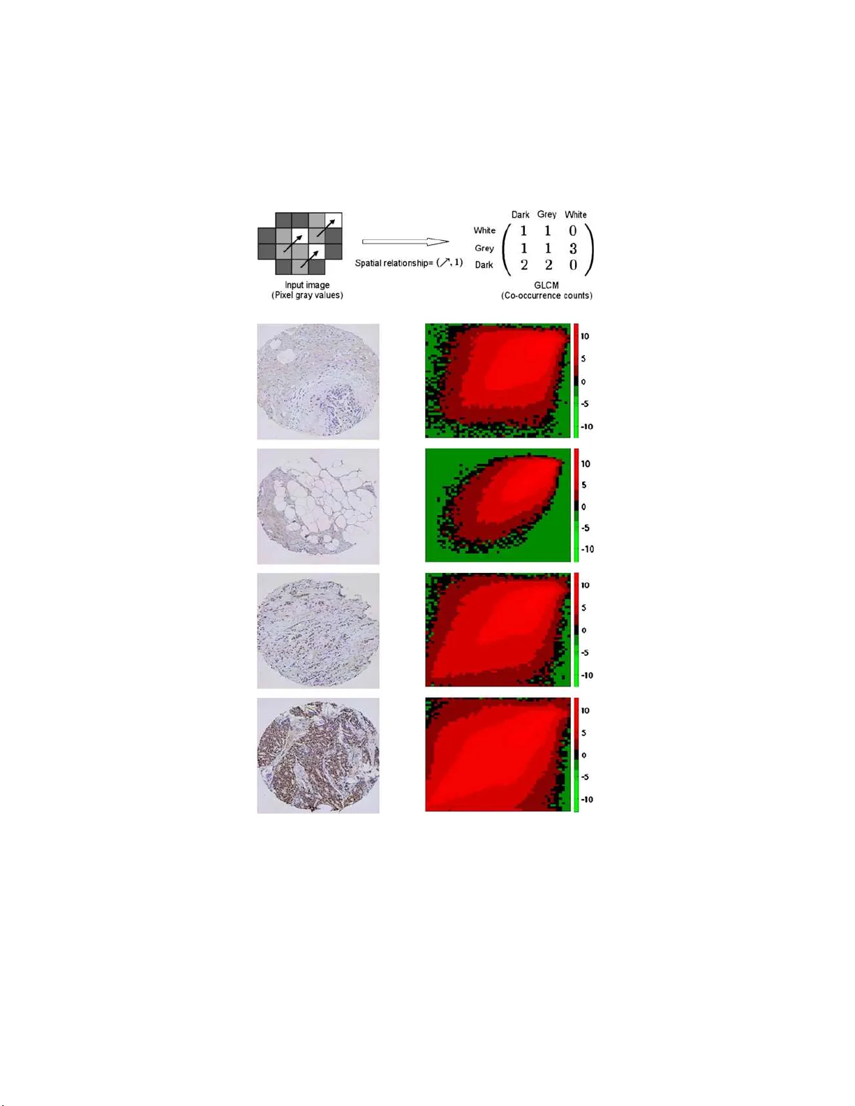
The Annals of Applie d Statistics 2012, V ol. 6, No. 3, 1280–130 5 DOI: 10.1214 /12-A OAS543 c  Institute of Mathematical Statistics , 2 012 ST A TISTICAL METHODS F OR TISSUE ARRA Y IMA GES—A LGORITHMIC SCORING AND CO-TRAINING By Donghui Y an, Pei W ang 1 , Michael Linden, Bea trice Knudsen and Timothy Randolph 1 F r e d Hutchinson Canc er R ese ar ch Center, F r e d Hutchinson Canc er R ese ar ch Center, University of Minnesota Me dic al Scho ol, Ce dars-Sinai Me dic al Center and F r e d H utchinson Canc er R ese ar ch Center Recent adv ances in tissue microarra y technolog y h ave allo wed im- munohistochemis try to b ecome a p ow erful medium- to-high through- put analysis to ol, particularly for th e va lidation of diagnostic and prognostic biomarke rs. How ever, as study size gro ws, the manual ev aluation of these assa ys b ecomes a prohibitiv e limitation; it v astly reduces throughpu t and greatly increases vari abilit y and exp en se. W e prop ose an algorithm—Tissue Array Co-Occurrence Matrix Analysis (T ACOMA)—for quantifying cellular p henotypes based on textu ral regularit y summarized by lo cal inter-pixel relationships. The algo- rithm can be easily trained for any staining pattern, is absent of sensitiv e tuning p arameters and has t h e ability to rep ort salien t pix- els in an image that con tribute to its score . P ath ologists’ input via informativ e training patches is an important asp ect of the algorithm that allow s the training for any sp ecific marker or cell type. With co-training, the error rate of T A COMA can be reduced substantially for a very small training sample (e.g., with size 30). W e give the- oretical insights into the success of co-training via thinnin g of the feature set in a high-d imensional setting when there is “sufficient” redundancy among th e features. T A COMA is flexible, transp arent and p ro vides a scoring pro cess that can b e ev aluated with clarit y an d confidence. In a stud y b ased on an estrogen receptor (ER) marker, w e sho w that T A COMA is comparable to, or outp erforms, p ath ologists’ p erformance in terms of accuracy and repeatability . Received January 2011; revised Jan uary 2012. 1 Supp orted in part by the follo wing Grants for th e National Institute of H ealth: R01CA126205 , R01GM082802 , U1CA086368, P01CA053996. Key wor ds and phr ases. Classification, ratio of separation, high-dimensional inference, co-training. This is an electronic reprint of the orig inal article published b y the Institute o f Ma thema tical Statistics in The Annals of Appli e d Statistics , 2012, V ol. 6, No. 3, 1 280–1 305 . This reprint differs from the orig inal in pagination and typog raphic detail. 1 2 D. Y AN ET AL. Fig. 1. Il lustr ation of the TMA te chnolo gy and example TMA i mages. T he top p anel is r eprinte d fr om Kononen et al. ( 1998 ) by c ourtes y of the Natur e Publishing Gr oup and it shows the steps i nvolve d in how a TM A image may b e pr o duc e d. The b ottom p anel di splays example TMA images with the numb ers in the left indic ating the sc or e of images in the same r ow. 1. In tro d uction. Tissue microarray (TMA) tec hnology w as fir st describ ed b y W an, F ortuna and F urmanski ( 1987 ) and substantia lly impr o ve d by Kononen et a l. ( 1998 ) as a high-throughpu t tec hn ology for the assessment of protein expression in tissue samp les. As s ho wn in th e to p panel of Figure 1 , the construction of a TMA b egins with cylindrical co res extracted from a donor blo c k of formalin-fixed and paraffin-emb ed ded tissues. T he cores are transferred to th e grid of the recipien t blo ck. This grid is generated b y punching cylindrical h oles at equal d istance into a precast r ectangular mold of solid paraffin wax. Once all the holes are filled w ith donor cores, the blo ck is h eated to fuse th e cores to the w ax of the blo c k. Normally , r ecipien t blo c ks con tain 360 to 480 tissue cores from d onor b lo cks, often in trip late samples from eac h blo c k and are th u s called tissue micro arrays (TMA). They are sectioned tr an s v ersely and eac h section is captured on a glass slide, suc h T ACOMA 3 that slides displa y a cross section of eac h core in a grid -lik e fashion. More than 100 slides can b e generated fr om eac h TMA b lo c k for analysis w ith a separate p r ob e. This pro cedure standard izes the h y b ridization pro cess of the prob e across h u ndreds of tissu e samples. The use of TMAs in cancer biology has increased dr amatical ly in r ecen t yea rs [Camp, Neumeister and Rimm ( 2008 ), Giltnane and Rimm ( 2004 ), Hassan et al . ( 2008 ), V o du c, Ken- ney and Nielsen ( 2008 )] for the rapid ev aluation of DNA, RNA an d protein expressions on large num b ers of clinical tissue samples; they remain the most efficien t method for v alidating proteomics data and tissue biomark ers. W e limit ou r discuss ion to high-density imm unohisto c hemistry (IHC) stain- ing, a metho d us ed for the measuremen t of protein exp ression, as the most common method for su b cellular lo calization. The ev aluation of pr otein expression requires the qu an tification, or scor- ing, of a T MA image. The scores can b e used for the v alidatio n of biomarkers, assessmen t of th er ap eutic targets, analysis of clinical outco me, etc. [Hassan et al. ( 2008 )]. The b ottom panel of Figure 1 giv es an examp le of s ev eral TMA images with scores assigned at a 4-p oint scale (see Section 4 for details). Although the construction of TMAs has b een automated for large-scale in terr ogation of markers in tissue samples, sev er al factors limit the use of the TMA as a h igh-throughput assay . These include the v ariabilit y , su b- jectivit y an d time-in tensive effort inherent in the visual scoring of staining patterns [Camp, Neumeister a nd Rimm ( 2008 ), V rolijk et al. ( 2003 )]. Indeed, a pathologist’s score r elies on su b jectiv e judgments ab out colors, textures, in tensities, d ensities and spatia l relationships. As n oted in Giltnane and Rimm ( 2004 ), how ev er, th e h u man ey e cannot pro v id e an ob jectiv e qu an tifi- cation that can be normalized to a reference. In ge neral, problems stemming from the sub j ectiv e and inconsisten t scoring by pathologists are well kn o wn and ha ve b een highligh ted by sev eral stud ies [Bentze n , Buffa and Wilson ( 2008 ), Berger et al. ( 2005 ), DiVito and C amp ( 2005 ), Kir k egaard et al. ( 2006 ), Thomson et al. ( 2001 ), W alk er ( 2006 )]. Thus, as s tu dy size gro ws, the v alue of T MAs in a r igorous statistical analysis ma y actually decrease without a consisten t and ob jectiv e scoring pro cess. These concerns ha v e motiv ated the recent dev elopmen t of a v ariet y of to ols for automated scoring, ranging from soph isticated image enhancement to ols, tissu e segmen tation to compu ter-assisted pathologist-based scoring. Man y are f o cused on a particular cellular pattern, with HER2 (exhib iting n u clear staining) b eing the most commonly targeted mark er; see, for exam- ple, Hall et al. ( 2008 ), Joshi et al. ( 2007 ), Masmoudi et al. ( 2009 ), Sk aland et al. ( 2008 ), T awfik et al. ( 2005 ). F or a survey of commercial systems, we refer to Mulrane et al. ( 2008 ) or Ro jo, Bueno and Slo dko wsk a ( 2009 ), and also the review by C regger, Berger and Rimm ( 2006 ) whic h ac kno wledges that, giv en the rapid c h anges in this field, this inform ation may become out- dated as devices are abandoned, improv ed or n ewly dev elop ed . A pr op ert y of most automated T MA scoring algorithms is that they rely on v arious 4 D. Y AN ET AL. forms of bac kground subtr action, feature segment ation and thresholds for pixel in tensit y . T uning of these algorithms can b e difficult and ma y resu lt in mod els sensitiv e to sev eral v ariables, including staining qualit y , bac k- ground an tib o dy bind ing, coun terstain intensit y , and the color and hue of c hr omogenic reaction pro ducts used to detect ant ib o dy b inding. Moreo v er, suc h algorithms t yp ically require tunin g f rom the v endors with parameters sp ecific to the markers’ staining pattern (e.g., n uclear v ersus cytoplasmic), or ev en require a dedicated p erson for suc h a system. T o address the fu r ther need f or scoring of TMAs in large b iomark er stud- ies, w e p rop ose a framew ork— called Tissue Arra y Co-Occurrence Matrix Analysis (T ACOMA)—that is trainable to any staining p attern or tissue t yp e. By seeking texture-based patterns in v arian t in the images, T ACOMA do es not rely on intensit y thresh olds, colo r filters, image segmen tation or shap e recognition. It r ecognizes s p ecific staining patterns b ased on exp ert input v ia a preliminary set of image patc hes. I n addition to p r o viding a score or categorizatio n, T ACOMA allo ws to see whic h pixels in an image con- tribute to its score. Th is clearly enhances in terpretabilit y and co nfidence in the results. It sh ould b e n oted that T A COMA is not d esigned for clinical diagnosis but rather a to ol for us e in large clinical studies that in volv e a range of p oten tial biomark ers. S ince man y th ou s ands of samples ma y b e required, the cost and time requ ired for pathologist-based scoring may b e prohibitive and so an efficien t automated alternativ e to human scoring can b e essenti al. T A COMA is a framew ork for such a purp ose. An imp ortan t concern in biomedical studies is that of the limited training sample size. 2 The size of the training set may nece ssarily b e small d ue to the cost, time or human efforts required to obtain them. W e adopt co-training [Y aro wsky ( 1995 ), Blum and Mitc h ell ( 1998 )] in the context of T A COMA to sub s tan tially red uce the training sample size. W e explore the thinn ing of the f eature set for co-training when a “natural” split is not readily a v ailable but the features are f airly redund an t, and this is sup p orted by our theory that a thinned slice carries ab out the s ame classification p o wer as the whole feature set und er some conditions. The organization of th e remainder of this pap er is as follo ws. W e describ e the T A C O MA algorithm in Section 2 , this is follo wed b y a d iscussion on co-training to reduce the training sample size with some theoretical insigh ts on the thinning sc h eme in Section 3 . Then in S ection 4 , w e presen t ou r exp erimenta l r esu lts. W e conclude with a d iscussion in Section 5 . 2. The T A C OMA algorithm. T h e p rimary chall enge T ACOMA addresses is the lac k of easily-quan tified criteria for scoring: features of int erest are not lo calized in p osition or size. Moreov er, within an y region of relev ance— 2 The additional issue of label noise was studied elsewhere [Y an et al. ( 2011 )]. T ACOMA 5 one con taining p rimarily cancer cells—there is no w ell-defined (quant ifiable) shap e that charact erizes a pattern of staining (see, e.g., the b ottom panel of Fig ure 1 for an illus tr ation). The k ey insigh t that un derlies T A C OMA is that, despite the h eterogeneit y of TMA images, they exhibit strong statisti- cal regularit y in the form of visually observ able textures or staining p attern [see, e.g., Figure 2 (b)]. An d, with the guidance of pathologists, T A CO MA can b e trained for this pattern regardless of the cancer cell type (breast, prostate, etc. ) or marker type (e.g. , nucleus, cytoplasmic, etc .). T A COMA captures the texture patterns exhibited by TMA images through a matrix of coun ting statistics, the Gra y Lev el Co-o ccurrence Matrix (GLCM). Through a small n umb er of represen tativ e image patc hes, T A COMA con- structs a feature mask so that the algorithm will fo cus on those b iologi cally relev an t features (i.e., a subset of GLCM entrie s). Besides s coring, T ACOMA also rep orts salien t image pixels (i.e., those cont ribute to the scoring of an image) whic h will b e usefu l for the purp ose of tr ainin g, comparison of m ul- tiple TMA images, estimation of staining in tensity , etc. F or the rest of this section, we will br iefly discuss these individual bu ilding blo c k s of T ACOMA follo w ed b y an algorithmic description of T A COMA. 2.1. The gr ay level c o-o c curr enc e matrix. The GLCM wa s originally pro- p osed by Ha ralic k ( 1979 ) and has prov en successful in a v ariet y of remote- sensing applications [Y an, Bic k el and Gong ( 2006 )]. The GLC M, of an image, is a matrix whose en tries co u n t the frequency of transitio ns b et wee n pixel in- tensities across neighboring pixels with a particular spatial relationship; see Figure 2 . Th e description here is essentia lly adopted fr om Y an, Bic ke l and Gong ( 2006 ). W e start by defining the sp atial relationship b etw een a pair of pixels in an image . Definition. A spatial relationship h as t wo elemen ts, the direction and the distance of in teraction. The s et of all p ossible spatial relationships is defined as ℜ = D ⊗ L = {ր , ց , տ , ւ , ↓ , ↑ , → , ←} ⊗ { 1 , . . . , d } , where D is th e set of p oten tial directions and L is the distance of interac tion b et ween the p air of pixels in volv ed in a spatial r elationship. T h e distance of in teraction is th e minimal n umb er of steps r equired to mo v e from one p ixel to the other along a given direction. The particular spatia l r elationships used in our application are ( ր , 3), ( ց , 1) and ( ր , 1). Details about the c h oice of these spatial relationships can b e seen in S ection 4 . Although th e defi n ition of spatial relationships can b e extended to inv olv e more pixels [Y an, Bic k el and Gong ( 2006 )], we ha v e fo cused on pairwise relationships whic h app ear to b e sufficien t. Next we define the GLCM. 6 D. Y AN ET AL. (a) (b) Fig. 2. Example images and their GLCMs. (a) Gener ating the GLCM fr om an image. This toy “image” (left) has 3 gr ay levels, { Dark , Gr ey , White } . Her e, under the sp atial r elationship ( ր , 1) , the tr ansition fr om Gr ey to W hite (indic ate d by ր ) o c curs thr e e tim es; ac c or dingly, the entry of the GLCM c orr esp onding to the Gr ey r ow and White c olumn has a value of 3 . (b) Example TMA images. I mages of a tissue sample (left p anel) and the He atmap (right p anel) of their GLCM (in lo g sc ale). The GLCM matric es ar e al l 51 × 51 ; e ach GLCM c el l in the he atmap indic ates the fr e quency of the c orr esp onding tr ansition. The c ol or sc ale is il lustr ate d by the c olor b ar on the right. T ACOMA 7 Definition. Let N g b e the num b er of gray lev els in an image. 3 F or a giv en image (or a patc h) and a fi xed s p atial relationship ∼ ∈ ℜ , the GLCM is defined as A N g × N g matrix suc h that its ( a, b )-en tr y coun ts the n umb er of pairs of p ixels, w ith gray v alues a and b , resp ectiv ely , ha ving a spatial rela- tionship ∼ , for a, b ∈ { 1 , 2 , . . . , N g } . This d efinition is illustr ated in Figure 2 (a) with more realistic examples in Figure 2 (b). Figure 2 (b) giv es a clear indication as to ho w the GLCM distinguishes b et wee n TMA images h a ving differen t staining patterns. Our use of the GLCM is nonstand ard in that w e do n ot use an y of the common scalar-v alued summaries of a GLCM [see Haralic k ( 1979 ) and Con- ners and Harlo w ( 1980 )], but instead employ the en tire matrix (with mask- ing) in a classification algorithm [see also Y an, Bic ke l and Gong ( 2006 )]. A GLCM ma y hav e a large n um b er of entries, t yp ically thousands, how ev er, the exceptional capabilit y of Random F orests [Breiman ( 200 1 )] in feature selection allo ws us to directly use all (or a mask ed sub s et of ) GLC M entries to d etermine a final score or classificat ion. 2.2. Image p atches for domain know le dge. In order to in corp orate p rior kno wledge ab out the staining pattern, we mask the GLCM matrix so that the scoring will fo cus on biologically p ertinen t features. T he masking is realized by firs t c ho osing a set of image patc hes representing regions that consist predominantly of cancer cells and are c hosen to r epresen t the staining patterns; see Figure 3 . The collection of GLCMs from these p atc hes are then used to define a template of “significan t entries” (cf. T ACOMA algorithm in Section 2.5 ) for all futu re GLCMs: wh en the GLC M of a n ew image is formed, only the en tries that corresp ond to this template are retained. This masking step enforces the idea that f eatures us ed in a classifier should not b e based on stromal, arterial or other nonp ertinent tissue whic h may exhibit nonsp ecific or backg round staining. Note that only one small s et of image patc hes is required; these imag e patc hes are us ed to p ro duce a common feature mask whic h is applied to all images in b oth training and scoring. In this fashion, feature selection is in itiated by exp ert biological kno w l- edge. This manner of feature selection inv olv es little human effort but leads to su bstan tial gain in b oth inte rpretabilit y and accuracy . Th e underlyin g phi- losoph y is that no mac hine learning algorithms sur pass d omain kno wledge. Since b y using image patc hes w e do not indicate whic h features to select but 3 Often b efore the computing of GLCM, the gray level of each p ix el in an image is scaled linearly from [1 , N o ] to [1 , N g ] for N o the predefined num b er, typically 256, of gra y lev els in the image. 8 D. Y AN ET AL. Fig. 3. R epr esent ative image p atches and the induc e d fe atur e m ask. F our p atholo gist– chosen p atches (left p anel) and the fe atur e mask as det ermine d by al l p atches (right p anel, se e algorithmic description of T ACOMA). Nonwhite entries i n this m atrix indic ate the c orr esp onding GLCM entries to b e use d in sc oring. Note that one and only one f e atur e mask i s r e quir e d thr oughout. instead sp ecify their effe ct, we ac hiev e the b enefits of a man u al-based feature selection bu t a void its difficulty . This is a no v el form of nonparametric, or implicit, feature selection whic h is app licable to settings b ey ond TMAs. 2.3. R andom for ests. T A COMA uses Random F orests (RF) [Breiman ( 2001 )] as the un derlying classifier. RF was pr op osed by Breiman an d is considered one of the best classifiers in a high-dimensional setting [Caruana, Karampatziakis and Y essenalina ( 2008 )]. In our exp erience, RF ac hiev es sig- nifican tly better p erformance th an SVM and Bo osting on the TMA images w e use (see T able 1 ). Additionally Holmes, Kap elner and Lee ( 2009 ) argue that RF is su p erior to others in d ealing with tissue images. The fund amen- tal building blo c k of RF is a tree-based classifier whic h can b e nonstable T able 1 Performanc e c omp arison of RF, SVM and Bo osting of a naive Bayes classifier. The r esult f or RF is adopte d fr om Se ction 4.1 . F or SVM , we vary the choic e of the kernel fr om { Gaussian, p olynomial, sigmoi d } wi th the b est tuning p ar ameters for N g ∈ { 7 , 9 , 13 , 26 , 37 , 51 , 64 , 85 } and the b est r esult is r ep orte d. F or b o osting, the b est r esult is r ep orte d by varying N g ∈ { 7 , 9 , 13 , 26 , 37 , 51 , 64 , 85 } and the numb er of b o osting iter ations fr om { 1 , 2 , 3 , 5 , 10 , 50 , 100 } Classifier Accuracy RF 78 . 57% SVM 65 . 24% Boosting 61 . 28% T ACOMA 9 Fig. 4. R andom F or ests classific ation. In th is il lustr ation the data p oints r eside in a unit squar e (left p anel). The two classes ar e indic ate d by r e d and blue dots. The true de cision b oundary i s the diagonal l i ne shown. RF (c enter p anel) gr ows many tr e es. Each tr e e c or- r esp onds to a r e cursive p artition of the data sp ac e. These p artitions ar e r epr esente d in the right p anel by a se quenc e of horizontal and vertic al lines; the data sp ac e shown her e is p artitione d by many instanc es. The RF classifier eventual ly l e ads to a de cision b oundary (solid black curve) for this two-class classific ation pr oblem. and sensitive to noise. RF tak es adv an tage of suc h instabilit y and creates a strong ensem ble b y b agging a large num b er of trees [Breiman ( 2001 )]. Eac h individual tree is gro wn on a b o otstrap sample from the training set. F or the splitting of tree no d es, RF randomly selects a num b er of candidate features or linear com bin ations of features an d splits th e tree no de with the one that ac hiev es th e most reduction in the no de impurity as defined b y the Gini index [or other measures su c h as the out of b ag (oob) estimat es of generalizat ion error] defined as follo ws: φ ( p ) = C X i =1 p i (1 − p i ) , (1) where p = ( p 1 , . . . , p C ) denotes the prop ortion of examples fr om different classes and C is the n u m b er of differen t classes. RF gro w s eac h tree to the maxim um and no p runing is requir ed. F or an illustr ation of RF, s ee Figure 4 . T o test a f u ture example X , let X fall from eac h tree for w hic h X re- ceiv es a v ote for the class of the terminal no de it reac hes. The fi nal class mem b ership of X is obtained by a ma jorit y v ote o v er the num b er of votes it receiv es for eac h class. Th e feat ures are r ank ed b y their resp ectiv e reduction of no de impur it y as m easured b y the Gini ind ex. Alternativ es includ e the p ermutati on-based measure, that is, p ermute v ariables one at a time and then r ank according to the resp ectiv e amount of d ecrease in accuracy (as estimated on o ob observ ations). 2.4. Salient pixels dete ction. A v aluable prop erty of T A C OMA is its abil- it y to rep ort salien t pixels in an image that d etermin e its score (see Figure 8 ). This prop ert y is based on a corresp ondence b et w een the p osition of pixels 10 D. Y AN ET AL. in an image and en tries in its GLCM, and made p ossible b y the remark- able v ariable-ranking capabilit y of RF. Here we use the imp ortance measure (Gini index-based) pr o vided by R F to rank the v ariables (i.e., entries of the GLCM) and then collect relev an t image pixels associated with th e imp ortant en tries. Since eac h en try of a GLCM is a coun ting statistic inv olving pairs of pixels, we can asso ciate the ( a, b )-entry of a GLCM with those pixels that mak e u p this GLCM en try . The set of imag e pixels that are asso ciated with the ( a, b )-en try of a GLCM is formally r epresen ted as G a,b = { x, y : x ∼ y , I ( x ) = a, I ( y ) = b } . In the ab o ve represen tation, x and y represent the p osition of image pixels and we treat an image I as a map from the p osition of an image pixel to its gra y v alue. Note that not all pairs of pixels w ith x ∼ y such th at I ( x ) = a, I ( y ) = b corresp ond to salient sp ots in a TMA image. Ho wev er, if the ( a, b ) -feature is “imp ortant” (e.g., as d etermined b y RF), then t yp ically most pixels in the set G a,b are relev an t. Whereas RF app ears to b e a blac k b o x—taking a large n u m b er of GLCM features and prod ucing a score—salien t pixels pro vide a quick p eek into its in tern als. Effectiv ely , RF works in roughly the same manner as a pathologist, that is, they b oth use salien t pixels to score the TMA images; th e seemingly m ysterious image features are mer ely a f orm of representa tion for use by a co m puter alg orithm. 2.5. An algorithmic description of T ACOMA. Denote the training sam- ple by ( I 1 , Y 1 ) , . . . , ( I n , Y n ) wh ere I i ’s are images and Y i ’s are s cores. Ad - ditionally , assume there is a set of L “representat iv e” image patc hes. The training of T ACOMA is describ ed as Algorithm 1 . In the ab o v e descrip tion, τ i is chosen as the median of en tries of matrix Z i for i = 1 , . . . , L . Then, for a new image, T A COMA will: (i) deriv e the GLCM matrix; (ii) s elect the en tr ies with indices in M ; (iii) app ly the trained clas- sifier on th e selected en tries and output the score. T he training and scoring with T ACOMA are illustrated in Figure 5 . 3. Co-training with RF. The sample size is an imp ortant issue in the scoring of TMA images, mainly b ecause of the high cost and human efforts in volv ed in obtaining a large sample of high qu alit y lab els. F or instance, it ma y tak e seve ral h ou r s for a well -trained pathologist to score 100 TMA im- ages. Unfortunately , it is often th e case that the classification p erformance drops sharp ly when the training samp le size is reduced. F or example, Fig- ure 6 shows the error rate of T A CO MA when the sample size v aries. O ur aim is to ac hiev e reasonable accuracy for small samp le size and co- training is adopted for this p u rp ose. T ACOMA 11 Algorithm 1 The training in T A COMA 1: for i = 1 to L d o 2: compute the GLCM f or the i th imag e patc h and denote by Z i ; 3: M i ← the ind ex set of Z i that surviv e thresholding at lev el τ i ; 4: end for 5: M ← S L j =1 M j ; 6: for k = 1 to n d o 7: compute the GLCM of image I k and k eep only en tries in index set M ; 8: denote the resulting matrix by X k ; 9: end for 10: F eed S n l =1 { ( X l , Y l ) } in to the RF classifier and obtain a classification rule. Co-training was prop osed in the landm ark pap ers by Y aro wsky ( 1995 ) and Blum an d Mitc hell ( 1998 ). It is an effectiv e wa y in training a m o del with an extremely small lab eled sample and has b een successfully applied in man y app lications [Blum and Mitc h ell ( 1998 ), Nigam and Ghani ( 2000 )]. The idea is to train tw o sep arate cla ssifiers (ca lled coupling classifiers) eac h on a different set of features using a small n umber of lab eled examples. Then the tw o classifiers iterativ ely tr ansfer those confi d en tly classified examp les, along with the assigned lab el, to the lab eled set. This pro cess is rep eated unt il all unlab eled examples h av e b een lab eled. F or an illustration of the idea of co -training, see Figure 7 . C o-training is r elev ant here due to the Fig. 5. T ACOMA i l lustr ate d. T he left and right p anels il l ustr ate, r esp e ctively, mo del tr aining and the use of the mo del on futur e data. 12 D. Y AN ET AL. Fig. 6. Err or r ate of T A COM A as the tr aining sample size varies. Ther e ar e 328 TMA images i n the test sample. natural r edundancy that exists among features that are based on GLCMs corresp onding to different spatial relatio nships. A learning m o de that is closely related to co-training is self-learning [Nigam and Ghani ( 2000 )], wh ere a single classifier is used in the “ lab el → tr ansfer → lab el ” lo op (cf. Figure 7 ). Ho w ever, emp ir ical studies ha ve sho wn that co-training is often sup erior [Nigam and Ghani ( 2000 )]; the intuitio n is that co-training allo ws the tw o coupling classifiers to pr ogressiv ely expand the “kno wledge b oundary” of eac h other w hic h is absen t in self-learning. Previous w orks in co-training use almost exclusiv ely Exp ectation Max- imization or Naive Ba yes based classifiers w here the p osterior p robabilit y serv es as the “confidence” required b y co-trai ning. Here w e use RF [Breiman ( 2001 )] w here the margin (to b e defin ed shortly) pro vided b y RF is used as a “natural” p r o xy for the “confid ence.” The margin is defin ed th rough the v otes r eceiv ed by an observ ation. F or an observ ation x in the test s et, let the n u m b er of vo tes it receiv es for the i th class b e denoted by N i ( x ) , i = 1 , . . . , C , Fig. 7. A n il lustr ation of c o-tr aining. T ACOMA 13 Algorithm 2 The co-t raining algorithm 1: while th e set U is not empty d o 2: for k = 1 , 2 do 3: T rain RF classifier f k on lab eled examples from L using feature set F k ; 4: Classify examples in the set U with f k ; 5: Under f k , ca lculate the margin for eac h obs erv ation in U ; 6: pic k m k observ ations, x ( k ) 1 , . . . , x ( k ) m k , with the largest margins; 7: end for 8: L ← L ∪ { x (1) 1 , . . . , x (1) m 1 , x (2) 1 , . . . , x (2) m 2 } ; 9: U ← U \ { x (1) 1 , . . . , x (1) m 1 , x (2) 1 , . . . , x (2) m 2 } ; 10: end while where C is the num b er of classes. The mar gin of x is defined as max i ∈{ 1 ,...,C } N i ( x ) − second j ∈{ 1 ,...,C } N j ( x ) , where se c ond in the ab o ve indicates the second-largest elemen t in a list. T o giv e an algorithmic d escription of co-training, let the tw o sub sets of features b e denoted by F 1 and F 2 , r esp ectiv ely . Let the set of lab eled and unlab eled examples b e denoted by L and U , resp ectiv ely . T h e co-training pro cess pro ceeds as Alg orith m 2 . The final error rate and class mem b ersh ip are d etermined by a fi xed coupling classifier, say , f 1 . W e set m 1 = m 2 = 2 in our experiments according to Blum and Mitc hell ( 1998 ). 3.1. F e atur e split for c o-tr aining. C o-training requires t wo subs ets of fea- tures (or a feature split). Ho wev er, co-training al gorithms rarely provi de a r ecip e for obtaining these f eature splits. There are sev eral p ossib ilities one can explore. The first is called a “natural” split, often resu lting from an un derstanding of the p roblem structure. A r ule of thum b as to what constitutes a natu- ral split is that eac h of the t wo feature subsets alone allo ws one to con- struct an acceptable classifier and that the tw o subsets somehow comple- men t eac h other (e.g., conditional indep endence giv en the lab els). F ortu- nately , TMA images represente d in GLCM’s naturally hav e su c h prop er- ties. F or a giv en problem, often there exist seve ral sp atial r elationships [e.g., ( ր , 3) and ( ց , 1) for T MA images studied in this work], with eac h inducing a GLCM sufficien t to constru ct a classifier w hile the “dep en dence” among the in duced GLCM’s is u sually low. Thus, it is ideal to apply co-training on TMA image s usin g such natural splits. When there is n o natural split readily a v ailable, one has to find tw o p rop er subsets of features. One w ay is via random splitting. C o-training via a ran- dom split of features w as initially considered by Nigam and Ghani ( 2000 ) but 14 D. Y AN ET AL. has since b een largely o verlook ed in the machine learning literature. Here w e extend the idea of r an d om splits to “thinning,” which is more fl exible and p oten tially may lead to a b etter co-training p er f ormance. Sp ecifically , rather than r an d omly sp litting the original feature set F = { 1 , . . . , p } in to t wo halves, w e sele ct tw o disjoin t subsets of F w ith size n ot necessarily equal bu t n on v anishing compared to p . Th is wa y of feature splitting leads to feature subsets smaller than F , hence the name “thinning.” One concrete implemen tation of this is to divide F into a num b er of, sa y , J , equal-sized partitions (eac h partition is also called a thinn ed slice of F ). In the f ollo wing discussion, unless otherw ise stated, thinnin g alw ays refers to this concrete implemen tation. It is clear that this includes random splits as a sp ecial case . Thinnin g allo ws one to constru ct a self-learning classifier (the features are tak en fr om one of th e J partitions), co-training (r an d omly pic k 2 out of J partitions) and so on. F or a giv en p roblem, one can exp lore v arious alterna- tiv es asso ciated with thin ning bu t here we shall fo cus on co-training. The extension of random split to thinning ma y lead to im p ro ved co- training p erformance, as thinning ma y mak e features fr om differen t p ar- titions less d ep endent and meanwhile well preserves the classificatio n p o we r in a h igh-dimensional setting wh en th ere is su ffi cien t redundancy among features (see S ection 3.2 ). Th e optimal num b er of partitions can b e selected b y heuristics suc h as the k ern el ind ep endence test [Bac h and Jordan ( 2003 ), Gretton et al. ( 2007 )], whic h w e lea v e for future w ork. 3.2. Some the or etic al insights on thinning. According to Blum and Mit- c hell ( 1998 ), one essent ial ingredien t of co-training is the “high” co nfidence of the tw o coupling classifiers in lab eling the u nlab eled examples. Th is is closely related to the strength of the tw o coupling classifiers w h ic h is in tur n determined b y the feature subsets inv olv ed. In this section, we stu d y how m u c h a thinned slice of the feature set F preserves its classification p o wer. Our r esult provi des in sigh t in to the n ature of thinning and is int eresting at its o wn right d ue to its close connection to s everal lines of in teresting w ork [Ho ( 1998 ), Dasgupta and Gup ta ( 2 002 )] in mac hine learning (see Sectio n 3.2.2 ). W e pr esen t our theoretical analysis in Section 3.2 .1 and list related w ork in Section 3.2.2 . In Sup plemen t A [Y an et al. ( 2012 )], we pr o vide additional sim u lation results related to our theoretica l analysis. 3.2.1. Thinning “pr eserves” the r atio of sep ar ation. Ou r th eoretical mo d el is the Gaussian mixture sp ecified as Π N ( µ 1 , Σ) + (1 − Π) N ( µ 2 , Σ) , (2) where Π ∈ { 0 , 1 } indicates the lab el of an observ atio n suc h that P (Π = 1) = π , and N ( µ , Σ) sta nds f or Gaussian distribution with mean µ ∈ R p and co- v ariance matrix Σ. F or simplicit y , we consider π = 1 2 and the 0–1 loss. W e will define the r atio of s ep aration as a measur e of th e fr action of “inf orm a- T ACOMA 15 tion” carried by the subset of features due to thinning with resp ect to that of the original feature set and show that this quan tit y is “preserved” up on thinning. F or simplicit y , we tak e J = 2 (i.e., rand om splits of F ) and similar discussion applies to J > 2 . Let the feature set F b e d ecomp osed as F = F 1 ∪ F 2 suc h that F 1 ∩ F 2 = ∅ and |F 1 | = p 2 , m. (3) W e will sh o w th at eac h of th e t wo subs ets of features, F 1 and F 2 , carries a substantia l fraction of the “information” cont ained in th e original data when p is large, assuming the data is generated from Gaussian mixture ( 2 ). A quantit y that is crucial in our inquiry is S F = u T F Σ − 1 F u F , (4) where u F = ( µ 1 − µ 2 ) F , ( U 1 , U 2 , . . . , U p ) F and her e F , as a su bscript, in- dicates that th e associated quantit y corresp onds to the f eature set F . W e call S F the sep aration of the Gaussian mixture induced by the fea ture set F . The separation is closely related to the Bay es error rate for classification through a wel l-kno wn result in multiv ariate statistics. Lemma 1 [And erson ( 1958 )]. F or Gaussian mixtur e ( 2 ) and 0–1 loss, the Bayes e rr or r ate is give n by Φ( − 1 2 ( u T F Σ − 1 F u F ) 1 / 2 ) wher e Φ( · ) is define d as Φ( x ) = R x −∞ 1 √ 2 π e − z 2 / 2 dz . Let the co v ariance matrix Σ b e w r itten as Σ =  A B T B D  , where we assume blo c k A corresp onds to features in F 1 after a p ermutati on of ro ws and columns. Ac cordingly , wr ite u as u F = ( u F 1 , u F 2 ) and define S F 1 (called the sep aration ind uced by F 1 ) similarly as ( 4 ). Now we can define the r atio of sep ar ation for the feature subset F 1 as γ = S F 1 S F . (5) T o see why definition ( 5 ) is usefu l, we giv e here a numerical example. Assume there is a Gauss ian mixtur e defined b y ( 2 ) su c h that Σ 100 × 100 is a tri- diagonal matrix with diago nals b eing all 1 and off-diag onals b eing 0 . 6, u F = (1 , . . . , 1) T . S upp ose one pic ks th e fir st 50 v ariables and form a new Gaussian mixture with co v ariance matrix A and mixtu re cen ter d istance u F 1 . W e wish to see ho w muc h is affected in terms of the Ba y es err or rate. W e h a ve S F = 45 . 87 , Φ( − 1 2 ( u T F Σ − 1 F u F ) 1 / 2 ) = 3 . 54 × 10 − 4 , S F 1 = 23 . 32 , Φ( − 1 2 ( u F 1 T A − 1 u F 1 ) 1 / 2 ) = 7 . 87 × 10 − 3 16 D. Y AN ET AL. and γ = 0 . 5084. Here the difference b etw een feature set F 1 and F is very small in terms of their classificatio n p o wer. In general, if the dimension is sufficien tly high and γ is nonv anish ing, then using a subset of features will not incur m uch loss in classificatio n p o wer. In Theorem 2 , w e will sho w that, under certain conditions, γ do es not v anish (i.e., γ > c for s ome p ositiv e constan t c ) so a feature subset is as go o d as the whole feature set in terms of cla ssification p o wer. Our main assumption (i.e., in Theorem 2 ) is actually a tec hnical one re- lated to the “lo cal” d ep endency among comp onents of u after some v ariable transformation. The exact context will b ecome clear later in the pro of of Theorem 2 . F or n ow, let Σ h a ve a Ch olesky d ecomp osition Σ = H H T for some lo w er triangular matrix H . A v ariable tr ansformation in the form of y = H − 1 u F will b e introdu ced. The idea is that w e desire Σ = H H T to p ossess a structur e su ch th at the comp onents of y = H − 1 u F are “lo cally” dep endent so that some form of la w of large n um b ers may b e ap p lied. T o a vo id tec h nical details in the m ain text , we shall discuss the assumption in the supplemen t [Y an et al. ( 2012 )]. Our m ain resu lt is th e follo w ing theorem. Theorem 2. Assume the data ar e gener ate d fr om Gaussian mixtur e ( 2 ). F urther assume the smal lest eigenvalue of Σ − 1 , denote d by λ min (Σ − 1 ) , is b ounde d away fr om 0 under p ermutations of r ows and c olumns of Σ . Then, under ass umptions of L emma 3 (c . f. Supplement A [Y an et al. ( 2012 )]), the sep ar ation induc e d by the fe atur e set F 1 satisfies S F 1 S F ≥  1 2  − in pr ob ability as p → ∞ wher e ( a ) − indic ates any c onstant smal ler than a . When the numb er of p artitions J > 2 , the right-hand side is r eplac e d by 1 /J . Pr oof. See supplemen t [Y an et al. ( 2012 )] for pro of.  3.2.2. R elate d work. There are m ainly tw o lines of work closely related to ours . One is the Johnson–Lin d enstrauss lemma and related [John son and Lindenstrauss ( 1984 ), Dasgupta and Gupta ( 2002 )]. T he Johnson–Lin d en- strauss (or J–L) lemma states th at, for Gaussian mixtures in high-dimensional space, up on a rand om pro jection to a lo w-dimensional sub space, the sepa- ration b etw een the mixtur e cen ters in the pr o jected space is “comparable” to that in th e original space with high p robabilit y . The d ifference is that the random p ro jection in J –L is carried out via a nontrivial linear trans- formation and the sep aration is d efined in terms of the Euclidean distance whereas, in our work, rand om pro jection is p erformed co ordinate-wise in the original space and w e define the separation with the Ma halanobis distance. T ACOMA 17 The other related work is the random sub space metho d [Ho ( 1998 )], an early v ariant of the RF classifier ensem ble algorithm, that is, comparable to b agging and Adab o ost in terms of empirical p erform an ce. T he r an d om subspace metho d gro w s a tree by randomly selecting half of the features and then co nstructs a tree-based classifier. Ho we ver, b ey ond sim ulations there has b een no formal justifi cation for the r an d om selectio n of half of the features. Our result pro vid es supp ort on this asp ect. In a high dimen- sional data setting where th e features are “redu ndant,” our resu lt sho w s that a randomly-selected half of the features can lead to a tree comparable, in terms of classification p ow er, to a classifier that uses all the features; m ean- while the random nature of the set of features used in eac h tree make s the correlation b etw een trees small, so go o d p erformance can b e exp ected. Our theoretica l result, when used in co-training, can b e view ed as a mani- festation of th e “blessings of the dimen s ionalit y” [Donoho ( 2000 )]. F or h igh- dimensional data analysis, the con v entio nal wisdom is to do dimension re- duction or pro jection pursuit. As a result, the “redun d ancy” among the features is t yp ically not used and, in man y cases, ev en b ecomes the n u isance one strives to get rid of. Th is is clearly a w aste. Wh en the “redu ndancy” among features is complemen tary , such redun dancy actually allo w s one to construct tw o coupling learners from w hic h co-training can b e carried ou t. It should b e emph asized that the splitting of th e fea ture set w orks b ecause of red undancy . W e b eliev e the exp loration of this t yp e of redun dancy will ha ve imp ortan t impact in high-dimensional data analysis. 4. Applications on TMA images. T o assess the p erformance of T ACOMA, w e ev aluate a collect ion of TMA images from the S tanford Tissue Microarray Database, or STMAD [see Marinelli et al. ( 2007 ) and h ttp://tma.sta nford. edu/ ]. TMAs corresp onding to th e p oten tial expression of the estrogen recep- tor (ER) protein in breast cancer tissue are used since ER is a histologically w ell-studied mark er that is expressed in the cell nucle us. An example of TMA images can b e seen in Figure 2 . Ther e are 641 TMA images in this set and eac h image has b een assigned a s core fr om { 0 , 1 , 2 , 3 } . The scor- ing criteria are as f ollo ws: “0 ” repr esen ting a d efi nite negativ e (no staining of cancer cells), “3” a definitiv e p ositiv e (a ma jority of cancer cells sho w dark n ucleus staining) and “2” for p ositive (a minorit y of cancer cells sh o w n u cleus staining or a ma jority sho w weak nucle us staining). Th e score “ 1” indicates am biguous w eak staining in a minority of cancer cells. Th e class distribution of the scores is (65 . 90% , 2 . 90% , 7 . 00% , 24 . 20%). Su c h an unbal- anced class distribution mak es th e scoring task eve n m ore c hallenging. In our experiments, w e assess the acc uracy b y the prop ortion of imag es in the test sample that receiv es the same sco re b y a scoring algorithm as that give n b y the reference set (e.g., ST MAD). W e split the images in to a training and a test set of sizes 313 and 328, resp ectiv ely . In the follo wing, we will first de- scrib e our choic e of v arious d esign options and parameters, and th en rep ort 18 D. Y AN ET AL. p erformance of T ACOMA o n a large training set (i.e., a s et of 313 TMA im- ages) and small training set (i.e., a set of 30 TMA imag es) with co-training in S ection 4.1 and Sectio n 4.2 , r esp ectiv ely . W e use three sp atial relationships, ( ր , 3), ( ց , 1) and ( ր , 1), in our ex- p eriments. In particular, ( ր , 3) is used in our exp eriment on T ACOMA for a large training set, wh ile ( ց , 1) is used along with ( ր , 3) in our co-training exp eriment and ( ր , 1) in an additional exp eriment (see T able 3 ). Often ( ր , 1) is the default choice in app licatio ns; w e u s e ( ր , 3) here to r eflect the gran u larity of the visual p attern seen in the images. I n deed, as the staining patterns in TMA images for E R m arkers o ccur only in the nucleus, ( ր , 3) leads to a sligh tly b etter scoring p erformance than ( ց , 1) according to our exp eriment on T ACOMA; moreo ver, no significant difference is observed for T ACOMA wh en simp ly concatenating features deriv ed from ( ր , 3) and ( ց , 1). ( ց , 1) is used in co-training in hoping that it is less correlated to features derived from ( ր , 3) than others, as these tw o are on the orthogonal directions. F or a go o d b alance of computational efficiency , discrimin ative p ow er, as w ell as ease of im p lemen tation, we take N g = 51 (our exp eriments are not particularly sensitive to the choi ce of N g in the range of 40 to 60) and apply uniform quan tization o v er the 256 gra y leve ls in our application. One ca n, of course, fu rther explore this, bu t w e wo uld n ot exp ect a sub stan tial gain in p erformance d ue to the limitation of a computer algorithm (or ev en h u man ey es) in distinguish ing su b tle differences in gra y lev els giv en a mo d erate sample size. W e use the R p ac k age “rand omF orest” 4 in this work. There are t wo im- p ortant paramete rs, the num b er of trees in the ens em ble and the n u m- b er of features to explore at eac h no d e split. These are searc hed thr ou gh { 50 , 100 , 200 , 500 } and { 0 . 5 √ p, √ p, 2 √ p } ( √ p is the default v alue suggested b y th e R pac k age for p the num b er of features fed to RF), resp ectiv ely , in this wo rk and th e b est test set error rates are rep orted. More information on RF can b e foun d in Breiman ( 2001 ). 4.1. Performanc e on lar ge tr aining set. The f ull set of 313 T MA images in the training set are used in this case. W e ru n T A CO MA on the training set (scores giv en by STMAD) and app ly the tr ained classifier to the test set im ages to obtain T ACOMA scores. Then, w e blind STMAD scores in the test set of 328 images ( 100 of which are duplicated so totally there are 428 images) and ha ve them r eev aluated by t wo exp erienced pathologists from t wo different in stitutions. The 100 duplicates allo w us to ev aluate the self-consistency of the pathologi sts. 4 Originally written in F ortran by Leo Breiman and Adele Cutler, and later p orted to R by A ndy Lia w and Matthew Wiener. T ACOMA 19 Although the scores from STMAD do not necessarily represent ground truth, they serv e as a fixed stand ard with resp ect to whic h the topics of accuracy and r epro ducibility can b e examined. On the test s et of 328 T MA images, T A CO MA achiev es a classification accuracy of 78 . 57% (accuracy defined as the prop ortion of images receiving the same score as ST MAD). W e argue this is close to the optimal. The Ba ye s r ate is estimated for this particular d ata example (repr esen ted as GLCMs) with a simula tion using a 1-nearest n eighb or (1 NN ) classifier. Th e Ba y es rate refers to the theo- retically b est classification rate giv en the data distribu tion. With the same training and test sets as RF classificatio n, the accuracy ac h iev ed b y 1 NN is around 60%. According to a celebrated theorem of Co ver and Hart ( 19 67 ), the err or r ate by 1 NN is at most twice that of the Ba ye s r ule. Th is result implies an esti mate of the Ba yes rate a t around 80% sub ject to sm all samp le v ariation (the estimated Bay es rates on the original image or its qu antized v ersion are all b oun ded ab ov e by this n umb er according to our simulation). Th us, T ACOMA is close to optimal. In the ab o ve exp eriments, w e u se four image patc hes. T o see if T A C OMA is sensitiv e to the c hoice of image p atc hes, we conduct exp eriments ov er a range of differen t p atc h sets and ac h iev e an a ve rage accuracy at 78 . 66 ± 0 . 52%. Such an accuracy ind icates that T ACOMA is robust to the c h oices of imag e patc hes. It is w orth r eemp h asizing that al l rep orts of test err ors for TMA images are n ot b ased on absolute tr uth, as all scores giv en to these images are sub jectiv ely pr o vided b y a v ariable h um an scoring pro cess. Salient sp ots dete ction. The abilit y of T A COMA to detect salient p ix- els is demonstrated in Figure 8 wher e image pixels are highlighte d in wh ite Fig. 8. The salient pixels (highlighte d in white). T he left p anel displays top fe atur es (indic es of GLCM entries) fr om the classifier wher e the x -axis and y -axis i ndi c ate the r ow and c olumn of the GLCM entr ies. The mi dd le and right p anels di splay images having sc or es 3 and 0, r esp e ctively; the pixels highlighte d i n white ar e those that c orr esp ond to the GLCM entries shown in the left p anel. Note the highlighte d pixels in th e right p anel ar e notably absent. F or visuali zation, only p art of the i mages ar e shown (se e Supplement B [Y an et al. ( 2012 )] f or lar ger images). 20 D. Y AN ET AL. Fig. 9. Classific ation p erformanc e of T ACOMA. On the STMAD test set T ACOMA achieves an ac cur acy of 78 . 57% . On the 142 images assigne d a unanimous sc or e by two p atholo gists and STMAD, T ACOMA agr e es on ab out 90% . if th ey are asso ciated with a s ignifi can t scoring feature. These highligh ted pixels are verified b y the pathologists to b e indicativ e. With r elativ ely few exceptions, these lo cations corresp ond to areas of stained nucle i in cancer cells. W e emphasize that these highligh ted p ixels indicate features most im- p ortant for classification as opp osed to id en tifying ev ery pr op ert y indicativ e of ER status. The highligh ted pixels facilitate in terpretation and the com- parison of images b y pathologists. The exp eriments with p atho lo gists. Th e sup erior classificatio n p erfor- mance of T ACOMA is also d emonstrated b y scores provi ded by the tw o pathologists. These t wo copies of scores, along with STMAD, pro vide three indep end en t pathologist-based scores. Am on g these, 142 images r eceiv e a u nanimous score. Consequently , these ma y b e v iewed as a r eference set of “true” scores against which the accuracy of T A C O MA migh t b e ev alu- ated (accuracy b eing defin ed as the prop ortion of images receiving th e same score as the reference set). Here, T A COMA ac h iev es an accuracy of 90 . 14%; see Figur e 9 . Scores provided by the tw o pathologists are also used to assess their self- consistency . Here self-consistency is defined as the p rop ortion of rep eated images receiving an identic al score b y the s ame pathologist. Consensus among differen t pathologists is an iss ue of concern [P enna et al. ( 1997 ), W alk er ( 2006 )]. In order to obtain information ab out the self-c onsistency of pathologist-based scores, 100 images are selected fr om th e set of 328 images. These 100 images are rotated and /or inv erted, and then mixed at random with the 328 images to a vo id recognitio n (so eac h pathologist actually scored a total of 428 TMA images). The self-consistency rates of the t wo patholo- gists are found to b e in the r ange 75– 84%. Of course, one desirable feature T ACOMA 21 of an y au tomated algorithm s u c h as T A CO MA is its complete (i.e., 100%) self-consistency . Performanc e c omp arison of RF to SVM and b o osting. The classification algorithm c hosen for T ACOMA is RF. Some p opu lar alternativ es include supp ort v ector machines (S VM) [Cortes and V apnik ( 1995 )], Boosting [F re- und and Sc h apire ( 1996 )] and Ba y esian netw ork [P earl ( 1985 )], etc. Using the same training and test set as that for RF, w e co nduct exp eriments with SVM as we ll as Bo osting of a naiv e Ba y es classifier. The input features for b oth SVM and Bo osting are the entries of the GLCM. W e use the Lib- svm [Chang and Lin ( 2001 )] soft ware for S VM. The naiv e Ba y es classifier is adopted from Y an, Bic ke l and Gong ( 200 6 ). T he idea is to find the cla ss that maximiz es the p osterior probabilit y for a new observ ation, den oted by ( I ( x ) = a x , x ∈ { 1 , 2 , . . . , N g } ⊗ { 1 , 2 , . . . , N g } ) for a fixed N g . Th at is, we seek to solve arg max k ∈{ 0 , 1 , 2 , 3 } Prob { k | I (1 , 1) = a 1 , 1 , . . . , I ( N g , N g ) = a N g ,N g } under the assu m ption th at ( I (1 , 1) , . . . , I ( N g , N g )) follo ws a m ultinomial dis- tribution. More details can b e found in Y an, Bic ke l and Gong ( 2006 ). The results are shown in T able 1 . W e can see that RF outp erforms S VM and Bo osting by a large margin. Th is is consisten t with observ ations made by Holmes, Kap elner and Lee ( 2009 ). 4.2. Exp eriments on smal l tr aining sets. W e conduct exp erimen ts on co - training with natural sp lits and thinning. F or natural splits, w e use GLC M’s corresp onding to t w o spatial relationships, ( ր , 3) and ( ց , 1), as features. F or thinning, we com b in e features corresp onding to ( ր , 3) and ( ց , 1) and then s plit this com bin ed feature set. The num b er of lab eled examples is fixed at 30 (compared to 313 in ex- p eriments with a large trainin g set). This choice is designed to make it easy to get a nonempty class 1 (wh ic h carries only ab out 2 . 90% of the cases). W e susp ect this num b er can b e furth er reduced withou t su ffering muc h in learning accuracy . The test set is the same as that in S ection 4.1 . The r e- sult is sho w n in T able 2 . One int eresting observ ation is that co-training by thinning achiev es an accuracy ve ry close to that by natural splits. Addi- tionally , T able 2 lists error rates giv en by RF on features corresp onding to ( ր , 3) ∪ ( ց , 1) an d its thinned sub sets. Here thinn ing of the feature set do es not cause m u c h loss in RF p erformance, consistent with our discu ssion in Section 3.2 . 4.3. Exp eriments of T ACOMA on additional data sets. Th is study fo- cuses on the ER mark er for w hic h the staining is nuclea r . Ho w eve r, the T A COMA algorithm can b e applied with equ al ease to mark ers that exhibit cell su r face, cytoplasm or other staining patterns. Add itional exp eriments 22 D. Y AN ET AL. T able 2 Performanc e of RF and c o-tr aining by thinning on TMA images. The unlab ele d set is taken as the test set in Se ction 4.1 and the lab ele d set is r andomly sample d fr om the c orr esp onding tr ai ning set. The subscript f or “thinning” indi c ates the numb er of p artitions. The r esults ar e aver age d over 100 runs and over the two c oupling classifiers f or c o-tr aining Scheme Error rate RF on ( ր , 3) ∪ ( ց , 1) 34.36% Thinning 2 on ( ր , 3) ∪ ( ց , 1) 34.21% Thinning 3 on ( ր , 3) ∪ ( ց , 1) 34.18% Co-training by natural split on ( ր , 3) and ( ց , 1) 27.49% Co-training by thinning 2 on ( ր , 3) ∪ ( ց , 1) 27.89% Co-training by thinning 3 on ( ր , 3) ∪ ( ց , 1) 27.62% are conducted on the S tanford TMA images corresp ondin g to three addi- tional protein markers: CD117, CD34 and NMB. These three sets of TMA images are selected for their large s ample size and relativ ely few missing scores (excluded from exp eriment). The results are sho wn in T able 3 . I n con trast, the automated scoring of cytoplasmic marke r s is often view ed as more d ifficult and refin ed commercial algorithms for these were r ep ortedly not a v ailable in a r ecen t ev aluatio n [Camp, Neumeister and Rimm ( 2008 )] of co mmercial scoring m etho ds. 5. Discussion. W e ha ve pr esen ted a new algorithm that automatica lly scores TMA images in an ob jectiv e, efficien t and repr o ducible manner. Our con tribu tions include the follo win g: (1) the use of co-occur r ence counting statistics to capture the spatial regularit y inherent in a heterogeneous and irregular set of T MA images; (2) the abilit y to rep ort salien t pixels in an im- age th at determine its score; (3) the incorp oration of p athologists’ input via informativ e training patc h es whic h mak es our algorithm adaptable to v arious T able 3 A c cur acy of T ACOMA on TMA im ages c orr esp onding t o pr otein markers CD117, CD34, NMB and ER. Exc ept f or ER (which has a fixe d tr aining and test set), we use ( ր , 1) and 80% of the i nstanc es for tr aining and the r est for test; this i s r ep e ate d for 100 runs and r esults aver age d Mark er Staining #Instances Accuracy ER Nucleus 641 78 . 57% CD117 Cell surface 1063 81.08% NMB Cytoplasmic 1036 84.17% CD34 Cytoplasmic and cell surface 908 76.44% T ACOMA 23 mark ers and cell t yp es; (4) a ve ry small training samp le is ac h iev ab le with co-training and w e h a v e pro vid ed some theoretica l ins igh ts into co -training via thinn ing of the f eature set. Ou r exp er im ents s ho w that T A CO MA can ac hiev e p erformance comparable to w ell-trained pathologists. It uses the similar set of pixels for scoring as that would be used by a pathologist and is not adv ersely sensitiv e to th e c hoice of image patc h es. The theory we ha ve dev elop ed on the thin ning sc heme in co-training giv es insights on why thin- ning may riv al the p erf ormance of a natur al split in co-training; a th inned slice m a y b e as goo d as the whole f eature set in terms of classification p o w er, hence, thinning can lead to t w o strong coup lin g classifiers that will b e used in co-training and this is what a natural s p lit ma y ac hiev e. The utilit y of T ACOMA lies in large p opulation-based studies that seek to ev aluate p oten tial m ark ers us in g IHC in large cohorts. Such a study m a y b e compr omised by a scoring pro cess, that is, protracted, prohibitive ly ex- p ensive or p o orly repro du cible. Ind eed, a manual scoring for such a study could require hundreds of hours of p athologi sts’ time without achieving a re- pro du cibly consisten t set of scores. Exp eriments with sev eral IHC marke rs demonstrate that our approac h has th e p oten tial to b e as accurate as man- ual scoring while pro viding a fast, ob jectiv e, inexp ensive and highly repr o- ducible alternative . Even more generally , T ACOMA ma y b e adopted to other t yp es of textur ed images su c h as those app earing in r emote sensing app li- cations. These p r op erties p r o vide ob vious adv anta ges for any sub sequen t statistica l analysis in determining the v alidit y or clinical utilit y of a p oten- tial mark er. Regarding r ep ro ducibilit y , w e note that the scores pr o vided b y t wo pathologists in our informal pilot study revea led an in tra-observe r agree- men t of arou n d 80% and an accuracy on ly in th e range of 70%, as defin ed b y the STMAD reference set (excluding all images deemed un s corable by the p athologi sts). Th is low inte r-observ er agreement may b e attribu ted to a v ariet y of factors, includ ing a lac k of a s ub jectiv e criteria used for s coring or the lac k of training against an established standard. This p erformance could su rely b e impro v ed up on, but it highligh ts the inh er ent sub j ectivit y and v ariabilit y of h uman-based s coring. In summary , T A COMA pro vid es a transparent scoring pr o cess that can b e ev aluated w ith clarit y an d confid en ce. It is also flexible with resp ect to mark er p atterns of cellular lo calizat ion: although the ER mark er is c harac- terized by staining of the cell nucleus, T A CO MA applies w ith comparable ease and su ccess to cytoplasmic or other marker staining patterns (see T a- ble 3 in Section 4.3 ). A soft wa r e implementati on of T A COMA is a v ailable up on request and the associated R p ac k age will b e made a v ailable to the R pr o ject. Ac kn owledgmen ts. Th e authors would lik e to thank the Asso ciate Editor and the anonymous review ers for their constructive comments and su gges- tions. 24 D. Y AN ET AL. SUPPLEMENT AR Y MA TERIAL Supp lemen t A: Assump tion A 1 , p ro of of Theorem 2 and simulati ons on thinning (DOI: 10.121 4/12-A OAS543SUPP A ; .p df ). W e p ro vide a detailed description of Assumption A 1 , a sk etc h of th e pro of of Theorem 2 and sim- ulations on the ratio of separation u p on thinn ing u nder different settings. Supp lemen t B: TMA images with salien t pixels marked (DOI: 10.1214 /12-A O AS543SUPP B ; .p df ). Th is su p plemen t con tains a close view of some TMA images where the salien t pixels are highlight ed. REFERENCES Anderson, T. W. (1958). An Intr o duction to M ultivariate Statistic al Analysis . Wiley , New Y ork . MR0091588 Bach, F. R . and Jordan, M. I. (2003). Kernel indep endent comp onent analysis. J. Mach. L e arn. R es. 3 1–48. MR1966051 Bentzen, S. M. , Buff a, F. M. and Wilson, G. D. (2008). Multiple biomarker tissue microarra ys: Bioinfor matics and practical approaches. Canc er Metastasis R ev. 27 481– 494. Berger, A. J. , Da v is, D. W. , T ellez, C. , Prieto, V. G. , Gershen w ald, J. E. , John- son, M. M. , Rimm, D. L. and Bar-Eli, M. (2005). Automated q uantitati ve analysis of activ ator protein-2alpha sub cellular expression in melanoma tissue microarra ys cor- relates with surviv al prediction. Canc er R es. 65 11185–1 1192. Blum, A. and Mitche ll, T . (1998). Combining lab eled and u nlabeled data with co- training. I n Pr o c e e dings of the El eventh Annual Confer enc e on Computa tional Le arning The ory (Madison, WI, 1998) 92–100. ACM, New Y ork. MR1811574 Breiman, L. (2001). Random Forests. Mach. L e arn. 45 5–32. Camp, R. L. , Neumeister, V. and Ri mm, D. L. (2008). A decade of tissue microarrays: Progress in the disco very and v alidation of cancer biomarke rs. J. Clin. Onc ol. 26 5630– 5637. Caruana, R. , Karamp a tziakis, N. and Yessenalin a , A. (2008). An empirical ev alua- tion of sup ervised learning in high dimensions. In Pr o c e e dings of the Tw enty-Fifth In- ternational Confer enc e on Machine L e arning (ICML), Helsinki, Finland 96–103. AC M, New Y ork . Chang, C. C. and Lin, C. J. (2001). LIBSVM: A library for support v ector machines. Av ailable at http://www .csie.ntu. edu.tw/ ~ cjlin/libs vm . Conners, R. and Harlo w, C. (1980 ). A theoretical comparison of texture algorithms. IEEE T r ansactions on Pattern Analyses and Machine Intel l i genc e 2 204–2 22. Cor tes, C. and V apnik, V. (1995 ). Supp ort vector netw orks. Machine L e arning 20 273– 297. Co ver, T . and Har t, P. (1967 ). Nearest neigh b or pattern classi fication. IEEE T r ansac- tions on Information The ory 13 21–27. Cregger, M. , Berger, A. and Rimm, D. (2006). Immunohistochemis try and quantita- tive analysis of protein exp ression. A r chives of Patholo gy & L ab or atory Me dicine 130 1026–10 30. Dasgupt a, S. and G upt a, A. (2002). An elementary pro of of the Johnson–Lindenstrauss lemma. R andom Structur es A lgorithms 22 60–65 . DiVito, K. and Camp, R. (2005). Tis sue microarra ys—automated analysis and future directions. Br e ast Canc er Online 8 . T ACOMA 25 Donoho, D. L. (2000). High-d imensional data analysis: The curses and blessings of dimen- sionalit y . Aide-Memoir e of a Le ctur e at AMS Confer enc e on Math Chal l enges of the 21st Century . Av ailable at http://w ww-stat.stanford.edu/˜donoho/Lectures/AMS20 00/ AMS2000.h tml . Freund, Y . and Schapire, R. E. (1996). Exp eriments with a new bo osting algorithm. In Pr o c e e dings of the Thirte enth International Confer enc e on Machine Le arning (ICML), Bari, I taly 148–15 6. Morgan Kaufman, San F rancisco, CA. Gil tnane, J. M. and Ri mm, D. L. (2004). T ec h n ology insight: Identification of biomarkers with tissue microarra y tec hnology. Nat. Clin. Pr act. Onc ol . 1 104–1 11. Gretton, A. , Fukumizu, K. , Te o, C. H. , S ong, L. , Sch ¨ olk opf, B. and Smola, A. J. (2007). A kernel statistical test of indep endence. In A dvanc es in Neur al I nf ormation Pr o c essing Systems (NIPS), V anc ouver, BC , Canada 585–592. MIT Pres s, Cam bridge, MA. Hall, B. H. , Ianosi-Irimie, M. , Ja vidia n , P. , Che n, W. , Ganesa n , S. and F oran, D. J. (2008). Co mputer-assisted assessmen t of the human epidermal grow t h factor receptor 2 imm unohisto c hemical assa y in imaged histologic sections using a mem- brane isolation algorithm and quantitative analysis of p ositive controls. BMC Me d. Imaging 8 11. Haralick, R. (1979). Statistical and structural app roac hes to texture. Pr o c e e dings of IEEE 67 786–803 . Hassan, S. , Ferrario, C. , Mamo, A. and Basik, M. (2008). Tissue microarra ys: Emerg- ing standard for biomark er v alidation. Curr. Opin. Bi ote chnol. 19 19–25. Ho, T. K. (1998). The random subsp ace method for constructing decision forests. IEEE T r ansactions on Pattern Analys is and Machine Intel ligenc e 20 832–844 . Holmes, S. , Kap elner, A. and Lee, P. ( 2009). An interactiv e JA V A statistical image segmen t ation system: GemIdent. Journal of Statistic al Softwar e 30 1–20. Johnson, W . B. and Lin denstrauss, J. (1984). Extensions of Lipschitz mappings into a Hilb ert space. I n Confer enc e in Mo dern Analysis and Pr ob ability (New Haven, Conn., 1982) . Contemp. M ath. 26 189–206. A mer. Math. Soc., Providence, RI. MR0737400 Joshi, A. S. , Sharangp ani, G . M. , Por ter, K. , K e yhani, S. , Morrison, C. , Basu, A. S. , Gholap, G. A. , G holap, A. S. and Barsky, S. H. (2007). S emi- automated imaging system to quantitate Her-2/neu membrane receptor immunoreac- tivity in human breast cancer. Cytometry Part A 71 273–285. Kirkegaard, T. , Edw ards, J. , Tovey, S . , McGl ynn, L. M. , Krishna, S. N . , Mukherjee, R. , T am , L. , Munro, A. F. , Dunne, B. and Bar tlett, J. M. S . (2006). Observer va riation in immunohistochemica l analysis of p rotein expression, time for a change? Hi stop atholo gy 48 787–794 . Ko n onen, J. , Bu bendorf, L. , Kallionimeni, A . , B ¨ arlund, M. , Schram l, P. , Leighton, S. , Torhorst, J. , Miha tsch, M . , Sauter, G. and Kallionimeni, O. (1998). Tissue microarra ys for h igh-throughput molecular profiling of tumor specimens. Natur e Me dicine 4 844–847. Marinelli, R. , Montgomer y, K. , Liu, C. , Shah, N. , Prapong, W . , Nitzberg, M. , Zachariah, Z. , Sherlock, G. , Na tkunam, Y. , West, R. et al. (2007). The Stanford tissue microarra y database. Nucleic A cids R es. 36 D871–D877. Masmoudi, H. , Hewitt, S. M. , Petri ck, N . , Myers, K. J. and Ga vrie li d es, M. A . (2009). Au tomated q uantitativ e assessmen t of H ER-2/neu immunohistochemica l ex- pression in breast cancer. IEEE T r ans. Me d. Imaging 28 916–92 5. Mulrane, L. , Rexhep aj, E. , Penney, S. , Callanan, J. J. and G alla gher, W . M. (2008). A utomated image analysis in histopathology: A va luable to ol in medical diag- nostics. Exp ert R ev. Mol. Diagn. 8 707– 725. 26 D. Y AN ET AL. Nigam, K. and Ghan i , R. (2000). Analyzing the effectiveness and applicability of co- training. In Pr o c e e dings of the Ninth International Confer enc e on Inf ormation and Know le dge M anagement, McL e an, V A 86–93. ACM, New Y ork. Pearl, J. (1985). Bay esian netw orks: A m o del of self-activ ated memory for evidential reasoning. In Pr o c e e dings of the Seven th Confer enc e of the Co gnitive Scienc e So ciety, Irvine, CA 329–33 4. Cognitive Science Soc., Austin, TX. Penna, A. , G rilli, R. , Filardo, G . , Mainin i, F. , Zola, P. , Mantov ani, L. and Libera ti, A. (1997). Do different physicians’ panels reac h similar conclusions? A case study on practice guidelines for limited surgery in b reast cancer. Eur op e an Journal of Public He alth 7 436–44 0. Ro jo, M. G. , Bueno, G . and S lodk owska, J. (2009). Review of imaging solutions for integ rated quantitative imm u nohistochemistry in the pathology daily practice. F oli a Histo chem. Cytobiol. 47 349–35 4. Skaland, I. , Øvest ad, I. , Janssen, E. A. M. , Klos, J. , Kj e llevo ld, K. H. , Hel- liesen, T. and Baak, J. (200 8). Digital image analysis improv es the quality of sub - jectiv e H ER-2 expression scoring in breast cancer. Applie d Immunohisto chemistry & Mole cular Morpholo gy 16 185–190 . T a wfik, O. W. , Kimler, B. F. , Da vis, M. , Donahue, J. K. , Persons, D. L. , F an, F. , Hagemeister, S. , Th omas, P. , Connor, C. , Jewell, W. et al. (2005). Compariso n of immunohistochemistry by automated cellular imaging system (ACIS) versus fluo- rescence in-situ hybridization in the ev aluation of H ER-2/neu expression in primary breast carcinoma. Histop atholo gy 48 258– 267. Thomson, T. A. , Ha yes, M. M. , Spinelli, J. J. , Hilland, E. , Sa wren k o, C. , Phillips, D. , Dupuis, B . and P arker, R. L. (2001). H ER -2/neu in breast cancer: Interobserv er v ariability and performance of immunohistochemistry with 4 anti b od ies compared with fluorescent in situ hybridization. Mo d. Pathol. 14 1079– 1086. Vo duc, D. , Ken ney, C. and Ni e lsen, T. O. (2008). Tissue microarrays in clinical on- cology . Semin. R adiat. Onc ol. 18 89–97. Vro lijk, H. , Sloos, W. , Mesker, W. , Fran ken, P. , F odde , R. , Morrea u, H . and T anke, H. (2003). Automated acquisitio n of stained tissue microarrays for high- throughput ev aluation of molecular targets. J. Mol. Di agn. 5 160– 167. W a lker, R. A. (2006). Quantification of imm u nohistochemistry—issues concerning meth- ods, utility and semiquantitativ e assessment I. Histop atholo gy 49 406–410. W a n, W. H. , For tuna, M. B. and Furmanski, P. (1987). A rapid and efficien t method for testing imm un ohistochemical reactivity of mono clonal an tib o dies ag ainst m ultiple tissue samples sim u ltaneously. J. Immunol. Metho ds 103 121–129. Y an, D. , Bickel, P. J. and Gong, P. (2006). A discrete log densit y expansion based approac h to Ikonos ima ge classification. In Americ an So ciety for Photo gr ammetry and R emote Sensing F al l Sp e ciality Confer enc e, San A ntonio, TX . Am. Soc. Photogramme- try and Remote Sensing, Bethesda, MD. Y an, D. , G ong, P. , Che n, A. and Zhong, L. (2011). Classification u nder data con- tamination with application to ima ge mis-registration in remote sensing. Av ailable at arXiv: 1101.35 94 . Y an, D. , W ang, P. , Lind en, M. , Knudsen, B. and Randolph, T. (2012). Supplement to “St atistical metho d s for tissue arra y images—algorithmic scoring and co-training.” DOI: 10.1214 /12-AO AS543SUPP A , D O I: 10.1214 /12-AO AS543SUPPB . Y aro wsky, D. (1995). U nsup ervised word sense d isam biguation riva ling sup erv ised meth - ods. In Pr o c e e dings of the 33r d Annual Me eting of the Asso ciation for Computational Linguistics, Cambridge, MA 189– 196. Morgan K aufmann, San F rancisco, CA. T ACOMA 27 D. Y an P. W a ng T. Randolph Biost a tistics and Bioma thema tics Program Fred Hutchinson Cancer Resear ch Center Sea ttle, W ashin gton 98109 USA E-mail: dy an@fhcrc.org p wa ng@fhcrc.org trandolp@fhcrc.org M. Linden Dep ar tment of Labora tor y Medicine and P a thology University of Minnesot a Medical School Minneapolis, Minnesot a 55455 USA E-mail: linde013@umn.edu B. Knudsen Dep ar tment of P a thology and Labora tor y Medicine Dep ar tment of Biomedical Sciences Cedars-Sinai M edical Center Los Angeles, California 900 4 8 USA E-mail: Beatrice.Kn udsen@cshs.org