Efficient Bayesian inference in stochastic chemical kinetic models using graphical processing units

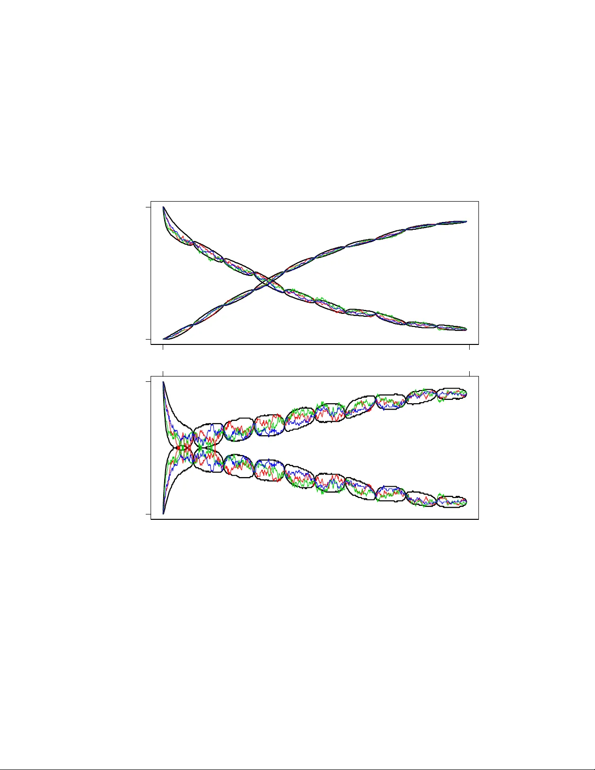
Efficien t Ba y esian inference in sto c hastic c hemical kinetic mo dels using graphical pro cessing units Jarad Niemi and Matthew Wheeler No vem ber 7, 2021 Abstract A goal of systems biology is to understand the dynamics of in tracellu- lar systems. Sto c hastic chemical kinetic mo dels are often utilized to accu- rately capture the sto c hastic nature of these systems due to low num b ers of molecules. Collecting system data allows for estimation of sto c hastic c hemical kinetic rate parameters. W e describe a w ell-known, but t ypically impractical data augmentation Marko v c hain Mon te Carlo algorithm for estimating these parameters. The impracticalit y is due to the use of rejec- tion sampling for latent tra jectories with fixed initial and final endp oints whic h can hav e diminutiv e acceptance probabilit y . W e show how graph- ical processing units can be efficien tly utilized for parameter estimation in systems that hitherto w ere inestimable. F or more complex systems, w e show the efficiency gain ov er traditional CPU computing is on the or- der of 200. Finally , we show a Ba yesian analysis of a system based on Mic haelis-Menton kinetics. 1 In tro duction The dev elopmen t of highly parallelized graphical pro cessing units (GPUs) has largely b een driven by the video game industry for faster and more accurate real-time 3D visualization. More recently the graphics card industry has intro- duced general purp ose GPUs for scien tific computing. Much of the fo cus of this w ork has b een on building parallelized linear algebra routines since these appli- cations are inherently amenable to parallelization [Galopp o et al., 2005, V olk ov and Demmel, 2008, Kr¨ uger and W estermann, 2005]. More recently the biolog- ical scien tific communit y has taken in terest for applications such as leuk o cyte trac king [Boy er et al., 2009], cluster identification in flo w cytometry [Suchard et al., 2010], and molecular dynamic simulation of in tracellular processes [Li and P etzold, 2010]. The statistics communit y has b een slo wer to v en ture into this massiv ely parallel area, but in the last couple of years a few pap ers hav e app eared us- ing GPUs to provide efficient analyses of problems that would otherwise by computationally prohibitiv e. T opics of these pap ers include statistical phylo- genetics [Suchard and Rambaut, 2009], slice sampling [Tibbits et al., 2010], 1 high-dimensional optimization [Zhou et al., 2010], simulation of Ising mo dels [Preis et al., 2009], appro ximate Bay esian computation (ABC) [Liep e et al., 2010], estimating multiv ariate mixtures [Suc hard et al., 2010], p opulation-based Mark ov chain Monte Carlo (MCMC) and sequen tial Monte Carlo metho ds [Lee et al., 2009]. As the num b er of parallel cores increase, the presence of GPU computing will undoubtably gro w. The use of parallel computing in the area of stochastic c hemical kinetics is primarily focused on sim ulation of systems assuming known reaction parameters [Li and P etzold, 2010]. Some ha v e used these sim ulations within an approximate Ba yesian computation (ABC) framew ork for estimation of reaction parameters [Liep e et al., 2010]. The Bay esian approach presented here is a sp ecial-case of the ABC methodology and can b e used as a gold-standard for comparing efficacy of the more general ABC metho dology . This approach implemen ts data augmen tation MCMC (D A-MCMC) where the latent tra jectories for chemical sp ecies are simulated at each iteration of the MCMC algorithm Marjoram et al. [2003]. Coupling this algorithm with GPU computing provides Monte Carlo estimates of parameter p osteriors for sizeable systems in reasonable time frames. This article pro ceeds as follows. In section 2, we describ e stochastic chemical kinetic models. In section 3, we introduce the D A-MCMC Bay esian approac h to parameter inference in these mo dels. Section 4 discusses mo difications required or beneficial for using this inferential technique on GPUs. Section 5 provides a sim ulation study to determine the com putational efficiency gain of using GPUs relativ e to CPUs as well as full Ba yesian analysis of a Mic haelis-Menton system. Finally , concluding remarks and future research plans are discussed in section 6. 2 Sto c hastic chemical kinetic mo dels Man y biological phenomenon can b e mo deled using sto chastic chemical kinetic mo dels Wilkinson [2006]. These mo dels are particularly useful when at least one sp ecies has a small num b er of molecules and therefore deterministic mo dels pro vide p o or appro ximations. In biology , this is common when considering in tra- cellular populations such as the n umber of DNA, RNA, and protein molecules. Belo w we introduce the notation required for understanding these sto c hastic c hemical kinetic models as w ell as metho ds used to simulate from them. Consider a spatially homogeneous bio c hemical system within a fixed v olume at constant temp erature. This system contains N species { S 1 , . . . , S N } with state vector X ( t ) = ( X 1 ( t ) , . . . , X N ( t )) 0 describing the n umber of molecules of eac h sp ecies at time t . This state v ector is updated through M reactions lab eled R 1 , . . . , R M . Reaction j ∈ { 1 , . . . , M } has a pr op ensity a j ( x ) = θ j h j ( x ) where θ j is the unknown sto chastic reaction rate parameter for reaction j and h j ( x ) is a known function of the system state x . Multiplying the prop ensit y b y an infinitesimal τ provides the probability of reaction j o ccurring in the in terv al [ t, t + τ ). If reaction j fires, the state vector is up dated to X ( t + τ ) = X ( t ) + v j where v j = ( v 1 j , . . . , v N j ) 0 describ es the num ber of molecules of eac h species 2 that are consumed or produced in reaction j . The probability distribution for the state at time t , p ( t, x ), is the solution of the chemic al master e quation (CME): ∂ ∂ t p ( t, x ) = M X j =1  a j ( x − v m ) p ( t, x − v m ) − a j ( x ) p ( t, x )  . (1) This solution is only analytically tractable in the simplest of models. In more complicated mo dels with discretely observed data, standard statistical metho ds for p erforming inference on the θ j s are una v ailable due to intractabilit y of this probabilit y distribution. This necessitates the use of analytical or numerical appro ximations such as approximate Bay esian computation [Marjoram et al., 2003]. 2.1 Sto c hastic sim ulation algorithm The DA-MCMC algorithm describ ed later requires forward simulation of the system from a known initial state which is accomplished using the sto c hastic sim ulation algorithm (SSA) [Gillespie, 1977]. The basis of this algorithm is the next r e action density function [Gillespie, 2001]: p ( τ , J = j | x t ) = a j ( x t ) a 0 ( x t ) · a 0 ( x t ) e − a 0 ( x t ) τ where a 0 ( x t ) = P M j =1 a j ( x t ). Since the join t distribution is the pr o duct of the marginal probability mass function for the reaction indicator j and the probabilit y density function for the next reaction time τ , the reaction indicator and reaction time are independent. SSA inv olv es sampling the reaction indicator J = j with probability a j ( x t ) /a 0 ( x t ) and the reaction time τ ∼ E xp ( a 0 ( x t )), where E xp ( λ ) is an exp onen tial random v ariable with mean 1 /λ . The state of the system is incremented according to the state change vector v j , time is incremen ted by τ , and the prop ensities are recalculated with the new system state. This pro cess con tinues un til the desired ending time is reached. Many sp eedups/appro ximations for SSA are av ailable and the reader is referred to Gillespie [2007] for a review. 3 Ba y esian inference Ba yesian inference is a methodology that describ es all uncertaint y through prob- abilit y . Let y denote an y data observed from the system and θ = ( θ 1 , . . . , θ M ) 0 the v ector of unknown parameters. The ob jective of a Bay esian analysis is the p osterior distribution that can b e found using Ba yes’ rule p ( θ | y ) = p ( y | θ ) p ( θ ) p ( y ) ∝ p ( y | θ ) p ( θ ) (2) 3 where p ( y | θ ) is the statistical mo del, often referred to as the lik eliho od, p ( θ ) is the prior distribution encoding information ab out the parameters av ailable prior to the curren t experiment, and p ( y ) is the normalizing constant to mak e p ( θ | y ) a v alid probability distribution. The second half of equation (2) indicates that it is rarely necessary to determine the normalizing constant p ( y ) when p erforming a Bay esian inference. 3.1 Complete observ ations In the unrealistic setting where the system is observed completely , i.e. y = X = X [0 ,T ] where X [ a,b ] indicates all v alues for X on the interv al [ a, b ], stochastic reaction rates can b e inferred easily . If w e assume independent gamma priors for eac h of the sto chastic reaction rates, i.e. θ j ind ∼ Ga ( α j , β j ), where the gamma distribution is proportional to θ α j − 1 j exp( − θ j β j ), then the p osterior distribution under complete observ ations are indep enden t gamma distributions θ j | y ind ∼ Ga ( α j + r j , β j + b j ) (3) where r j is the num be r of times reaction j fired and b j is the integral of h j ( · ) o ver interv al [0 , T ]. Mathematically , we write r j = K X k =1 I( j k = j ) b j = Z T 0 h j ( X t ) dt = K X k =1 h j ( X t k − 1 ) ( t k − t k − 1 ) (4) where j k ∈ { 1 , . . . , M } is the reaction index for the k th reaction, I( x ) is the indicator function that is 1 when x is true and 0 otherwise, t k is the time of the k th reaction, and a total of K reactions fired in the interv al [0 , T ]. The t wo v alues r j and b j are the sufficien t statistics for parameter θ j and are utilized in Section 4.3 to increase computational efficiency . 3.2 Discrete observ ations In the more realistic scenario of p erfect but discrete observ ations of the sys- tem, the problem b ecomes analytically intractable and, even worse, n umerical tec hniques are c hallenging [Wilkinson, 2006]. This challenge comes from the necessit y to simulate paths from X t i − 1 to X t i where t i − 1 and t i are consecutive observ ation times [Bo ys et al., 2008]. These simulated paths are necessary when using a Gibbs sampling approach presen ted in the following section that alter- nates b et ween 1) dra ws of parameters conditional on a tra jectory and 2) dra ws of tra jectories consistent with the data and conditional on parameters. W e define the discrete observ ations as y = { X t i : i = 0 , . . . , n } and up date Ba yes’ rule in equation (2) to include the unknown full latent tra jectories X . 4 The desired p osterior distribution is now the joint distribution for the underlying laten t states and the unknown parameters p ( θ , X | y ) ∝ I( y 0 = X t 0 ) p ( θ ) n Y i =1 I( y i = X t i ) p  X ( t i − 1 ,t i ] | θ , X t i − 1  = p ( θ ) n Y i =1 p  X ( t i − 1 ,t i ) | θ , X t i − 1 = y i − 1 , X t i = y i  where p  X ( t i − 1 ,t i ) | θ , X t i − 1 = y i − 1 , X t i = y i  denotes the distribution for the la- ten t state starting at y i − 1 and ending at y i o ver the time in terv al ( t i − 1 , t i ), i.e. the distribution for a con tinuous-time Mark o v chain with fixed endpoints. Since this distribution is not analytic – ev en up to a proportionality constan t – the distribution p ( θ , X | y ) is not analytic. 3.3 Mark o v chain Mon te Carlo A widely used technique to ov ercome these in tractabilities in Bay esian analysis is a to ol called Marko v chain Monte Carlo (MCMC). In particular, we utilize a sp ecial case of MCMC known as Gibbs sampling [Marjoram et al., 2003]. This iterativ e approach consists of tw o steps: 1. draw θ ( i ) ∼ p ( θ | X ( i − 1) , y ) and 2. draw X ( i ) ∼ p ( X | θ ( i ) , y ) where superscript ( i ) indicates that w e use the dra w from the i th iteration of the MCMC, p ( θ | X ( i − 1) , y ) is the distribution for the parameters based on complete tra jectories, and p ( X | θ ( i ) , y ) is the distribution for the complete tra jectory based on the current parameters. The join t draw  θ ( i ) , X ( i )  defines an ergo dic Marko v c hain with stationary distribution p ( θ , X | y ). In order to utilize this Gibbs sampling approac h, samples from the ful l c on- ditional distributions for θ and X are required, i.e. p ( θ | X , y ) and p ( X | θ , y ), resp ectiv ely . Recognize that p ( θ | X , y ) = p ( θ | X ) since y ⊂ X due to X rep- resen ting the en tire latent tra jectory at all time p oin ts as if w e had complete observ ations. Under complete observ ations, this full conditional distribution w as already provided in equation (3). Therefore, samples are obtained by cal- culating the sufficient statistics in equation (4) based on X rather than y and dra wing indep enden t gamma random v ariables for each reaction parameter. 3.3.1 Rejection sampling The full conditional distribution for X is, again, analytically intractable, but it is still p ossible to obtain samples from the distribution us ing r eje ction sampling [Rob ert and Casella, 2004, Ch. 2]. T o accomplish this, we use Bay es’ rule on the full conditional for X : p ( X | θ , y ) ∝ n Y i =1 p  X ( t i − 1 ,t i ) | θ , X t i − 1 = y i − 1 , X t i = y i  5 where p ( θ ) is subsumed in the prop ortionalit y constant. A rejection sampling approac h consistent with this full conditional distribution can b e p erformed indep enden tly for each interv al ( t i − 1 , t i ) for i = 1 , . . . , n as follows 1. forward simulate X on the in terv al ( t i − 1 , t i ) via SSA using parameters θ with initial v alue X t i − 1 = y i − 1 , and 2. accept the sim ulation if X t i is equal to y i otherwise return to step 1. As with any rejection sampling approach, the efficiency of this metho d is de- termined by the probability of forw ard simulation from X t i − 1 = y i − 1 using parameters θ resulting in X t i at time t i . F or these sto c hastic kinetic mo dels, this probabilit y can be very low and therefore w e aim to take adv antage of the massiv ely parallel nature of graphical pro cessing units to forw ard simulate many tra jectories in parallel until one tra jectory succeeds. 4 Adaptation to graphical pro cessing units P arallel pro cessing is clearly only adv an tageous if the co de is parallelizable. In the DA-MCMC algorithm, eac h step of the algorithm giv en in Section 3.3 can b e parallelized. The first step in volv es a join t draw for all stochastic reaction rate parameters conditional on a simulated tra jectory . These parameters can b e sampled indep endently as shown in equation (3). W e can conceptually send the sufficient statistics for eac h reaction off to its o wn thread to sample a new rate parameter for that reaction. The second step in volv es rejection sampling to find a tra jectory that satisfies in terv al-endp oin t conditions. Both of these steps are candidates for parallel processing. The theoretical maximum sp eed-up for parallel pro cessing versus serial pro- cessing is b ounded by Amdahl’s quan tity 1 / (1 − P + P /C ) where P is the p ercen tage of time sp en t in co de that can b e parallelized and C is the num b er of parallel cores av ailable [Amdahl, 1967, Suchard et al., 2010]. The first step in the DA-MCMC can only b e parallelized up to the minim um of M , the n umber of reactions, and C . With the chemical kinetic systems under consideration, M << C and therefore the gain from parallelizing this step is minimal. In con trast, the gain in parallelizing the rejection sampling step in DA-MCMC is en tirely dep enden t on the acceptance rate. As the acceptance rate drops, P → 1 and maximum p erformance gain from parallelization is achiev ed. In our appli- cation, the acceptance rate is often very lo w and therefore we focus on efficiency gained from parallelizing the rejection sampling step. Consider initially the goal of sampling a tra jectory from some initial state x 0 at time 0 given parameter θ to a final state x 1 in time 1. Using SSA, the probabilit y of sim ulating this tra jectory by starting at x 0 using parameter θ and attaining x 1 has probability p , whic h is generally unknown. The num- b er of simul ations required before a successful attempt is a geometric random v ariable with exp ectation 1 /p . Therefore as the probabilit y decreases, the ex- p ected n umber of runs increases and the system b ecomes amenable to parallel pro cessing. 6 A simple approach to parallelization is to hav e each computing thr e ad at- tempt one simulation and determine whether that simulation was successful, i.e. the final state is x 1 at time 1. If m ultiple threads are successful, then one of those simulations is sampled uniformly . The sufficient statistics for that sim ulation are calculated and the DA-MCMC can con tinue b y sampling rate parameters based on those statistics. In the follo wing subsections, we discuss the implementation details required to turn this simple idea into a an efficien t realit y . 4.1 Indep enden t pseudo-random n um b er streams Most curren t GPU-parallelized Monte Carlo algorithms know, prior to parallel k ernel inv ocation, how man y random num b ers will b e needed b y each thread and can therefore use a “skip-ahead” tec hnique [L’Ecuy er et al., 2002] for ob- taining indep endent streams of pseudo-random num b ers [Lee et al., 2009]. This tec hnique relies on one long pseudo-random num b er stream. The k ey idea is to hav e the next thread skip ov er the n random num b ers needed b y the thread b efore it. Unfortunately , in the SSA algorithm the num b er of random n umbers required for each thread is random and therefore this approach b ecomes infea- sible unless we are willing to settle for n sufficiently large to ensure a minuscule probabilit y of ov erlap in the sequences. Ev en then, we are inviting computa- tional inefficiency since the “skip-ahead’ requires O (log n ) op erations [L’Ecuyer et al., 2002]. Instead, w e use dynamic creation of pseudo-random num b ers Matsumoto and Nishim ura [2000] which has already b een used in the SSA context Li and P etzold [2010]. This metho d creates a set of pseudo-random n umber streams based on the Mersenne-Twister family of generators. A hypothesis concerning statistical indep endence of these streams is giv en in Matsumoto and Nishimura [2000]: ‘a set of PRNGs [pseudo-random n umber generators] based on linear recurrences is m utually “indep endent” if the characteristic p olynomials are rel- ativ ely prime to eac h other.’ These authors state that there are many PRNG researc hers who agree with this h yp othesis. T o balance memory constraints (discussed in Section 4.4) with execution sp eed, w e implemen t one “indep enden t” Mersenne-Twister (MT) p er warp , the set of threads that receive instructions simultaneously . Current generation GPUs hav e 32 threads p er w arp and, again balancing memory with execution, w e ha ve implemented MTs that utilize a set of 40 in tegers for calculation of pseudo-random num b ers. Figure 1 depicts threads within a warp accessing one MT. Within a warp, the first 20 threads execute simultaneously follo wed b y the remaining 12 in order to ensure prop er up dating of the MT. T o update the MT, thread i records the MT state integers at lo cations i , i +1 mo dulo (mo d) 40, i +20 mo d 40 (op erations sp ecific to this 40-in teger MT) Matsumoto and Nishimura [2000]. The thread p erforms bit-wise op erations on these in tegers and records the output as the up dated state at lo cation i Matsumoto and Nishimura [1998]. After all threads hav e completed, they compute the pseudo-random n umber required for the SSA algorithm. F or the following round of pseudo-random 7 n umbers, the threads are shifted with resp ect to the MT state such that thread i is now aligned with MT state i +32 mo d 40, a pro cess that contin ues ad infini- tum . After all threads within a w arp hav e completed the SSA algorithm, the MT state plus the last used state index are written to global memory for use in the following kernel inv o cation. Figure 1: A depiction of threads (black boxes, thread 1 is greyed) within a warp accessing Mersenne-Twister states (red boxes). A) The first 20 threads (threads 1 and 20 depicted) accessing states i , i + 1 mo d 40, and i + 20 mo d 40 where i is the tread id. B) These threads up date their corresp onding Mersenne-Twister state (filled red b o xes). C-D) Threads 21 to 32 now p erform steps A and B. E) F or the next round of pseudo-random n umbers, the threads shift so that thread 1 starts at the next Mersenne-Twister state to b e updated. 4.2 Bypass thread sim ulation Ideally once one thread is successful, curren t and future threads should b e ab orted. One asp ect of GPU computing that v aries from standard parallel pro cessing is that no assumption can b e made ab out the order in which threads o ccur. A statement such as ‘if all threads with global thread id less than i 8 ha ve failed, then p erform simulation’ cannot b e made since it is unknown which threads hav e already made an attempt. Nonetheless, the same effect can arise b y creating a global v ariable that indicates when a thread has b een successful, but care is required. A t any giv en time during the parallel execution of rejection sampling, threads can b e placed into three categories: alr e ady-c omplete d-and-faile d , in-pr o gr ess , and waiting-to-b e-exe cute d . Once an in-pr o gr ess thread is successful, it writes to global memory indicating that it was successful and stores its pseudo-random n umber state. F or alr e ady-c omplete d-and-faile d threads no efficiency gains are p ossible. F or waiting-to-b e-exe cute d threads a simple c heck at the onset of sim u- lation to the global success v ariable is sufficient to bypass the thread simulation if a thread has already b een successful. Finally , in-pr o gr ess threads could p eri- o dically c heck whether another thread has been successful, but this adds unnec- essary o verhead and, more imp ortan tly , could bias results. Instead, in-pr o gr ess threads are allow ed to complete ev en if another thread has been successful in the mean time. In the unlik ely even t that another thread is successful, it is added to the list of successful threads and at the completion of all threads one of the successful threads is sampled uniformly . 4.3 Sufficien t statistics A naive approach to recording the SSA tra jectory is to record the state and time when each reaction fires whic h requires N K + K integers/foats where K is the num ber of reactions that fired. A parsimonious wa y of representing a tra jectory is to record the initial state vector as w ell as the times and iden tity of eac h reaction and recreating the tra jectory when needed. The memory storage requiremen t for this approach is N + 2 K in tegers/floats. In addition, K is random and therefore memory management is required to deal with v arying arra y sizes. Recall that the full condition distribution for the rate parameters dep ends only on the sufficient statistics in equation (4). So rather than recording the en tire tra jectory , the sufficien t statistics can b e recorded whic h reduces the memory requiremen t down to 2 M integers/floats where, often, M ≈ N and K >> M . If inference on the tra jectories is required, then this can b e accom- plished after the DA-MCMC is complete by rerunning the rejection sampling for each (or a subset) of the MCMC iteration v alues for the rate parameters. A solution that reduces the memory requirements ev en further and do es not require rerunning the rejection sampling is to record the initial PRNG state that resulted in a successful sim ulation in lieu of b oth the full tra jectory and the sufficient statistics. The memory storage requirement is only 41 integers (40-in teger MT state plus the last used state index) whic h clearly scales with N , M , and K . F or calculation of sufficien t statistics or an y tra jectory inference, the tra jectory is re-simulated with parameters corresp onding to that iteration in the MCMC and using the initial PRNG state that was previously successful. 9 Figure 2: The CUDA memory model. 4.4 Efficien t memory usage A trade-off made for the massiv ely parallel nature of the GPU is the amount of memory av ailable for each thread. This is an ov erarching concern that has b een co vered elsewhere [Lee et al., 2009, Suchard et al., 2010], but w e no w discuss ho w this concern can b e addressed in the parallel rejection sampling framework. Figure 2 provides a diagram of the CUD A memory mo del. Imp ortan tly , an y access to memory below the threads (in green) is relativ ely slow and memory depicted ab ov e the threads is fast, but v ery limited. T able 1 pro vides hardware memory constrain ts on the T esla T10 GPU and the algorithm memory allocation describ ed here. Constant memory can be used for quan tities that do not change during the GPU kernel execution and has an 8k cache for efficien t access [Kirk and Hwu, 2009, Ch. 5]. Therefore it is a con venien t location for the stoic hiometry matrix and reaction rate parameters (whic h only change outside of the GPU k ernel) since these are common to all blo c ks and threads. Without considering efficient sparse matrix storage, the n umber of integers needed to store b oth the matrix and parameters is M ( N + 1) whic h, giv en the systems of in terest, easily fits within the constant memory cac he. After constant memory , efficien t memory access is achiev ed by utilizing reg- isters and shared memory . Registers are restricted to automatic scalar v ariables, i.e. not arrays, that are unique to each thread [Kirk and Hwu, 2009, Ch. 5]. If 10 T able 1: Relev ant hardware memory constraints in kilobits (in tegers) for the T esla T10 GPU and algorithm memory allo cation. Memory type Amoun t (integers) Algorithm allo cation Registers p er blo c k 32 × 512 Thread system time Thread lo op v ariables Shared p er SM 4 kb (8 × 512) Twister state during SSA sim ulation Thread system state † Thread reaction prop ensities † Lo cal p er thread 16 kb (4096) Thread system state † Thread reaction prop ensities † Global 4 Gb ( ≈ 10 9 ) Success counter Successful twister state Twister states when not in use Constan t 64 kb (16,384) Reaction rate parameters Stoic hiometry matrix † If shared memory is av ailable, thread system state and reaction propensities are mov ed from local to shared memory . w e are using the maximum n umber of threads p er blo c k of 512, then we are lim- ited to 32 registers. Clear candidates for register storage are system time in the SSA sim ulation and simple loop v ariables. T o determine the num ber of registers p er thread compile using the n vcc compiler option --ptxas-options=-v . The SSA algorithm currently uses all 32 registers p er thread and therefore allows us to use the maxim um of 512 threads p er blo ck. Shared memory is fast-access memory that can b e utilized by all threads within a blo c k. In this impleme n tation, we take adv antage of the fast-access by storing pseudo random num b er generator states. Also, dep ending on the system size, we can store eac h thread’s SSA current system state, an N -integer arra y , and p ossibly even the M -float arra y con taining the reaction prop ensities. The PRNGs take up 2560 bytes of shared memory p er blo c k leaving 13824 bytes left o ver to store the system state and/or the reaction prop ensities. Therefore, if N + M ≤ 6, then b oth the state and prop ensities can be stored, otherwise there is not enough memory av ailable to store b oth. This limitation can b e met b y either decreasing the num ber of threads p er blo c k to increas e the amoun t of a v ailable shared memory per thread or by using local or global memory . In our exp erience, the optimal metho d generally dep ends on the system b eing studied. Remaining v ariables are stored either in lo cal or global memory dep ending on whether they are thread-sp ecific or not. F or example, tw o important global v ariables include the indicator of whether a thread has b een successful and the arra y of successful MT states. 11 5 Sim ulation example W e compare the efficiency of a GPU implementation to con ven tional CPU im- plemen tation using the model Michaelis-Men ton mo del. This widely known mo del is describ ed by the following reaction graph: E + S θ 1 − * ) − θ 2 E S θ 3 − → E + P (5) where E is a protein enzyme, S is a substrate that is con verted into a product P , and E S is an in termediate sp ecies for this pro duction. The prop ensities for the three reactions are a 1 ( X ) = θ 1 E · S , a 2 ( X ) = θ 2 E S , and a 3 ( X ) = θ 3 E S where X = ( E , S, E S, P ). This system has tw o conserv ation of mass relationships: E 0 = E + E S and S 0 = S + E S + P . 5.1 GPU vs CPU F or comparing GPU vs CPU timing, we considered only the rejection sampling step in Section 3.3.1 of the D A-MCMC algorithm rather than the entire MCMC algorithm. This w as done since the probability of rejection is highly dep enden t on the current MCMC parameter draws and to obtain accurate timing a large quan tity of MCMC iterations is required to eliminated timing bias due to ex- ploration of the parameter p osterior. Unfortunately , obtaining a reasonable quan tity of MCMC iterations on the CPU is simply not feasible on a reasonable time scale. Therefore, we compare timing for the rejection sampling p ortion of the algorithm only , although we expect the efficiency gain for the GPU should b e comparable if the entire MCMC timing could b e analyzed. It is imp ortan t to note that if the rejection sampling step had no rejections, then w e w ould exp ect the CPU to p erform comparable to the GPU and possibly ev en b etter if GPU ov erhead is considerable. Therefore it is of interest to study the efficiency gain as a function of the difficulty of the rejection sampling step. Figure 3 compares the efficiency of one core of a 2.66GHz Intel Xeon CPU vs one T esla T10 GPU where increasing difficulty of rejection sampling is equiv alent to increased exp ected dra ws. F or high acceptance probability rejection sampling sc hemes, the efficiency gain is mo dest and may not b e worth the trouble of con- v erting co de to GPU use. In contrast for lo w acceptance probabilit y rejection sampling sc hemes, the efficiency gain is around 200, meaning the GPU version will p erform 200 times faster than the CPU version. The efficiency gain ap- p ears to hit an asymptote around 200, for our algorithm implementation while the computation time in volv ed app ears to be exp onentially increasing as the ac- ceptance probability decreases. Therefore incredibly low acceptance probability rejection sampling sc hemes could still not b e handled on a GPU, but may be suitable to simultaneous use of multiple GPUs. 12 10 20 50 100 200 Expected samples (log 10 ) CPU/GPU system time 3 4 5 6 0.01 0.1 0.5 GPU time per iteration (seconds) Figure 3: The multiplicativ e increase in rejection sampling efficiency (blac k) and the GPU time for one iteration (red) with 95% interv als (dashed) for one core of a 2.66GHz In tel Xeon CPU vs a T esla T10 GPU. The effect of expected n umber of samples required for eac h acceptance w as studied by holding constant θ 2 = 0 . 001 and θ 3 = 0 . 1 while increasing θ 1 from 0.001 to 0.00245 in the Michaelis-Men ton system of equation 5. 5.2 Ba y esian inference The ultimate goal of this Bay esian analysis is p erforming inference in sto c hastic c hemical kinetic mo dels on b oth the unknown reaction rate parameters and the laten t tra jectory betw een data p oin ts. The Michaelis-Men tion system was sim ulated with true parameters θ 1 = 0 . 001, θ 2 = 0 . 2, and θ 3 = 0 . 1 from time 0 up to time 100. The data used are pro vided in T able 2 where both the E S - complex and product P are initialyl zero. Through the monotonic decrease in S , it is clear this system conv erts the substrate in the pro duct. The enzyme quan tity initially decreases drastically as it b onds to av ailable substrate, but then as substrate is con verted to product more un b ound enzyme is av ailable. T able 2: Measuremen ts tak en from a simulated Michaelis-Men tion system with parameters θ 1 = 0 . 001, θ 2 = 0 . 2, and θ 3 = 0 . 1. Time 0 10 20 30 40 50 60 70 80 90 100 E 120 71 76 81 80 90 90 104 103 109 109 S 301 219 180 150 108 86 61 52 35 29 22 13 A non-informative indep enden t prior is assumed for all reaction rate param- eters, namely p ( θ ) ∝ ( θ 1 θ 2 θ 3 ) − 1 . This prior is found as the limit of the gamma priors when b oth the shap e and rate parameters approach zero, but the gamma p osterior of equation (3) is still prop er with α j = β j = 0 ∀ j if each reaction o ccurs at least once. The DA-MCMC algorithm w as run for 10,000 burn-in iterations and then another 40,000 iterations were used for inference. Con vergence was monitored informally via traceplots and formally using the Gelman-Rubin diagnostic [Gel- man and Rubin, 1992, Bro oks and Gelman, 1997]. While lack of conv ergence is detected, samples are discard as burn-in . Post burn-in, no lac k of con vergence w as detected. Figure 4 provides p osterior histograms for the reaction rate parameters based on the observ ations in T able 2. The biv ariate con tour plot of θ 1 and θ 2 indicate that the v alue θ 1 + θ 2 is estimable from the data, but the individual v alues for θ 1 and θ 2 are hard to estimate. This identifiabilit y issue is common in systems biological parameter inference where equilibrium reactions ab ound. One adv an tage of Ba yesian analyses is trivially obtained estimates and un- certain ties for any function of the mo del parameters. Figure 4 provides p osterior histograms for b oth K D = θ 2 /θ 1 and K M = [ θ 2 + θ 3 ] /θ 1 kno wn as the disso- ciation constant and Michaelis constant, resp ectively . Although many metho ds ha ve b een dev elop ed to estimate the Michaelis constant, dating at least to the Linew eav er-Burk plot from 1934 Linewea v er and Burk [1934], few metho ds pro- vide an uncertain ty on the estimate. Based on the plot in Figure 4, there is 95% probabilit y that the true is in the range 246 to 343. Figure 5 pro vides p oin t-wise credible interv als for the four Mic haelis-Menton system sp ecies. Due to mass conserv ation, w e see that E and E S are mirror opp osites of eac h other and S and P are very close to being mirror opp osites of each other. The scien tific questions of interest that are answ ered by these tra jectories include when was the S → P c onversion 90% c omplete? or what is the pr ob a bility that E S cr osse d the 90 mole cule thr eshold? Ba y esian analyses can trivially answ er these questions while it remains difficult for other statistical metho ds. 6 Discussion W e presented a Ba yesian analysis of sto c hastic chemical kinetic mo dels that utilize a data augmen ted MCMC algorithm where the augmentation infers la- ten t tra jectories sampled via rejection sampling. This dramatic increase in efficiency when utilizing a GPU will allo w for analysis of v astly larger systems in reasonable amoun ts of time. The timing comparison in this manuscript only compared rejection sampling and therefore the results are biased sligh tly in fa v or of the GPU. F urther work is required to explore the efficiency gain of the entire MCMC, but we susp ect the results to b e v ery similar to the results presented here and the b enefit of letting the CPU algorithm run for months is marginal. The observ ations in this man uscript were discrete but perfect. Clearly this 14 is an unrealistic scenario in practical applications since we rarely obtain p erfect observ ations of the underlying system. Realistic mo dels naturally incorporate error in one of t wo w a ys: 1) the true v alue is within a threshold of that observ ed or 2) all v alues are possible but v alues closer to that observed are more probable. In the first approach, everything discussed in this man uscript is still applicable since forw ard simulations that are consisten t with the observ ations will still b e needed. These simulations could easily b e harder to obtain and therefore more amenable to parallelization. In the second approac h, all tra jectories are p ossibilities and therefore rejection sampling is not applicable. W e are exploring the use of an indep enden t Metrop olis-Hastings prop osal and methodologies that exploit creation of m ultiple indep enden t prop osals simultaneously . Appro ximate Ba yesian computation approaches hav e already b een imple- men ted on a GPU in a pac k age called ABC-SysBIO [Liep e et al., 2010]. This w as implemented in Python utilizing the PyCUDA wrapp er[Kl¨ oc kner et al., 2009] to access the CUDA API. Since Liep e et al. [2010] devotes only tw o para- graphs relev an t to this manuscript, it is unclear ho w PyCUDA implements the algorithm, e.g. random num ber generation, memory efficiency , etc., and whether it is comp etitiv e with the implementation discussed in this manuscript. The few pap ers discussing Bay esian inference on GPUs published to date ha ve shown remark able efficiency gains. Since this field is computation heavy , this increased efficiency should lead to Bay esian techniques b eing muc h more widely adopted than they are to da y as the capacity to solv e highly complex problems in reasonable time frames increases. 7 Ac kno wledgemen ts The authors gratefully ackno wledge supp ort from NSF IGER T Grant DGE- 0221715 and the Institute for Collab orativ e Biotechnologies through contract no. W911NF-09-D-0001 from the U.S. Arm y Researc h Office. The conten t of the information herein does not necessarily reflect the p osition or p olicy of the Go vernmen t and no official endoresemen t should be inferred. References G.M. Amdahl. V alidit y of the single pro cessor approach to achieving large scale computing capabilities. In Pr o c e e dings of the April 18-20, 1967, spring joint c omputer c onfer enc e , pages 483–485. A CM, 1967. Mic hael Boy er, David T arjan, Scott T. Acton, and Kevin Sk adron. Accelerating leuk o cyte trac king using cuda: A case study in leveraging man ycore coproces- sors. Par al lel and Distribute d Pr o c essing Symp osium, International , 0:1–12, 2009. doi: http://doi.ieeecomputersociety .org/10.1109/IPDPS.2009.5160984. R. J. Bo ys, D. J. Wilkinson, and T. B. Kirkw o o d. Ba yesian inference for a discretely observed sto c hastic kinetic model. Statistics and Computing , 15 18(2):125–135, 2008. ISSN 0960-3174. doi: http://dx.doi.org/10.1007/ s11222- 007- 9043- x. Stephen P . Bro oks and Andrew Gelman. General metho ds for monitoring con- v ergence of iterative sim ulations. Journal of Computational and Gr aphic al Statistics , 7(4):434–455, 1997. N. Galoppo, N.K. Govindara ju, M. Henson, and D. Manocha. LU-GPU: Effi- cien t algorithms for solving dense linear systems on graphics hardware. In Pr o c e e dings of the 2005 ACM/IEEE c onfer enc e on Sup er c omputing , page 3. IEEE Computer So ciet y , 2005. Andrew Gelman and Donald B. Rubin. Inference from iterative sim ulation using m ultiple sequences. Statistic al Scienc e , 7(4):457–472, 1992. ISSN 08834237. URL http://www.jstor.org/stable/2246093 . Daniel T. Gillespie. Exact sto c hastic simulation of coupled chemical reactions. Journal of Physic al Chemistry , 81(25):2340–2361, 1977. Daniel T. Gillespie. Sto chastic simulation of c hemical kinetics. Annual R eviews in Physic al Chemistry , 58:35–55, 2007. D.T. Gillespie. Approximate accelerated sto c hastic simulation of chemically reacting systems. The Journal of Chemic al Physics , 115:1716, 2001. D. Kirk and W. Hwu. Programming massively parallel pro cessors. Sp e cial Edition , page 92, 2009. A. Kl¨ oc kner, N. Pinto, Y. Lee, B. Catanzaro, P . Iv ano v, and A. F asih. Py- CUD A: GPU run-time co de generation for high-p erformance computing. A rxiv pr eprint arXiv , 911, 2009. J. Kr ¨ uger and R. W estermann. Linear algebra op erators for GPU implementa- tion of n umerical algorithms. In ACM SIGGRAPH 2005 Courses , page 234. A CM, 2005. Pierre L’Ecuy er, Richard Simard, E. Jack Chen, and W. David Kelton. An ob ject-oriented random-num b er pack age with many long streams and sub- streams. Op er ations R ese ar ch , 50(6):pp. 1073–1075, 2002. ISSN 0030364X. URL http://www.jstor.org/stable/3088626 . A. Lee, C. Y au, M.B. Giles, A. Doucet, and C.C. Holmes. On the utility of graphics cards to p erform massiv ely parallel simulation of adv anced mon te carlo metho ds. Pr eprint , 2009. H. Li and L. P etzold. Efficien t parallelization of the sto c hastic simulation al- gorithm for chemically reacting systems on the graphics pro cessing unit. In- ternational Journal of High Performanc e Computing Applic ations , 24(2):107, 2010. 16 J. Liep e, C. Barnes, E. Cule, K. Erguler, P . Kirk, T. T oni, and M.P .H. Stumpf. ABC-SysBio–appro ximate Bay esian computation in Python with GPU sup- p ort. Bioinformatics , 26(14):1797, 2010. H. Linewea ver and D. Burk. The determination of enzyme disso ciation con- stan ts. Journal of the Americ an Chemic al So ciety , 56(3):658–666, 1934. P . Marjoram, J. Molitor, V. Plagnol, and S. T av ar´ e. Mark ov c hain Monte Carlo without likelihoo ds. Pr o c e e dings of the National A c ademy of Scienc es of the Unite d States of A meric a , 100(26):15324, 2003. M. Matsumoto and T. Nishim ura. Mersenne twister: a 623-dimensionally equidistributed uniform pseudo-random num b er generator. ACM T r ansac- tions on Mo deling and Computer Simulation (TOMAC S) , 8(1):3–30, 1998. ISSN 1049-3301. M. Matsumoto and T. Nishimura. Dynamic creation of pseudorandom num ber generators. In H. Niederreiter and J. Spanier, editors, Monte Carlo and Quasi- Monte Carlo Metho ds 1998 , pages 56–69. Springer-V erlag, Berlin, 2000. T. Preis, P . Virnau, W. Paul, and J.J. Sc hneider. GPU accelerated Mon te Carlo sim ulation of the 2D and 3D Ising mo del. Journal of Computational Physics , 228(12):4468–4477, 2009. Christian P . Robert and George Casella. Monte Carlo Statistic al Metho ds . Springer Inc, 2 edition, 2004. ISBN 978-0-387-21239-5. M.A. Suchard and A. Rambaut. Many-core algorithms for statistical ph yloge- netics. Bioinformatics , 25(11):1370, 2009. M.A. Suchard, Q. W ang, C. Chan, J. F relinger, A. Cron, and M. W est. Under- standing GPU programming for statistical computation: Studies in massively parallel massiv e mixtures. Journal of Computational and Gr aphic al Statistics , 19(2):419–438, 2010. Matthew Tibbits, Murali Haran, and John Liec h ty . Parallel m ultiv ariate slice sampling. Statistics and Computing , pages 1–16, 2010. ISSN 0960-3174. URL http://dx.doi.org/10.1007/s11222- 010- 9178- z . 10.1007/s11222- 010-9178-z. V. V olk ov and J.W. Demmel. Benc hmarking GPUs to tune dense linear algebra. In Pr o c e e dings of the 2008 ACM/IEEE c onfer enc e on Sup er c omputing , pages 1–11. IEEE Press, 2008. Darren J. Wilkinson. Sto chastic Mo del ling for Systems Biolo gy . Chapman & Hall/CR C, London, 2006. H. Zhou, K. Lange, and M.A. Suc hard. Graphics pro cessing units and high- dimensional optimization. Arxiv pr eprint arXiv:1003.3272 , 2010. 17 θ 1 p( θ 1 |y) 0.000 0.002 0.004 0.006 0 2000 4000 6000 8000 θ 2 p( θ 2 |y) 0.0 0.5 1.0 1.5 2.0 0 1000 2000 3000 4000 5000 θ 3 p( θ 3 |y) 0.07 0.09 0.11 0 500 1000 1500 2000 2500 θ 1 θ 2 0.001 0.003 0.005 0.007 0.0 0.5 1.0 1.5 2.0 x K D p(K D |y) 0 50 150 250 0 500 1000 1500 K M p(K M |y) 250 300 350 400 0 200 400 600 800 1000 1200 Figure 4: P osterior histograms for sto c hastic reaction rate parameters as well as the sto c hastic disso ciation and Michaelis constants, K D = θ 2 /θ 1 and K M = [ θ 2 + θ 3 ] /θ 1 resp ectiv ely , and a biv ariate contour plot (quantiles: 2.5%, 25%, 50%, 75%, and 95%) for the joint p osterior of θ 1 and θ 2 with true v alues (red) based on the data in T able 2 and using the DA-MCMC algorithm. 18 0 100 0 300 Time Substrate Product 0 120 Enzyme ES−comple x Figure 5: Posterior 95% p oin t-wise credible interv als (blac k) and three random dra ws from the p osterior (colored) for the state tra jectory . 19