Tuning Time-Domain Pseudospectral Computations of the Self-Force on a Charged Scalar Particle

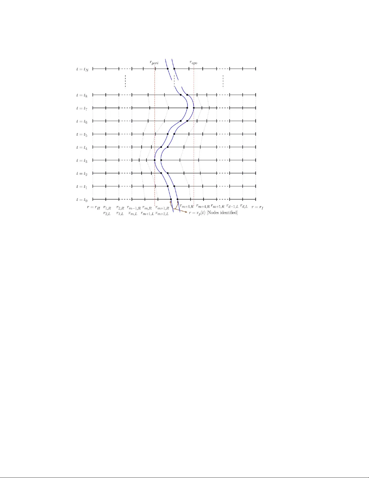
T uning Time-Domain Pseudosp ectral Computations of the Self-F orce on a Charged Scalar P article Priscilla Canizares and Carlos F. Sopuerta Institut de Ciències de l’Espai (CSIC-IEEC), F acultat de Ciències, Campus UAB, T orre C5 parells, Bellaterra, 08193 Barcelona, Spain E-mail: pcm@ieec.uab.es, sopuerta@ieec.uab.es Abstract. The computation of the self-force constitutes one of the main challenges for the construction of precise theoretical wa veform templates in order to detect and analyze extreme-mass-ratio inspirals with the future space-based gravitational-w av e observ atory LISA. Since the num b er of templates required is quite high, it is important to develop fast algorithms b oth for the computation of the self-force and the production of wa veforms. In this article w e show ho w to tune a recent time-domain technique for the computation of the self-force, what we call the Particle without P article scheme, in order to make it v ery precise and at the same time v ery efficient. W e also extend this technique in order to allow for highly eccentric orbits. P A CS num bers: 04.20.-q,04.25.Nx,04.30.Db,02.70.Hm AMS classification scheme num b ers: 35Q75,65M70,83C10 Submitted to: Class. Quantum Gr av. T uning Time-Domain Pseudosp e ctr al Computations of the Self-F or c e 2 1. In tro duction Gra vitational W av e Astronomy has the p oten tial to un veil the secrets of physical phenomena not yet understo o d inv olving strong gravitational fields. In order to realize this p oten tial there are observ atories/detectors either operating or b eing design/constructed that co ver a significant part of the relev ant gravitational-w av e frequency spectrum. F rom the v ery low band ( 10 − 9 − 10 − 6 Hz), where we hav e the pulsar timing arrays to the high frequency band ( 1 − 10 4 Hz), where most ground- based detectors op erate. In low frequency band ( 10 − 4 − 1 Hz), not accessible from the ground, w e find the future Laser Interferometer Space Antenna (LISA) [1], an ESA-NASA mission consisting of three spacecrafts forming a triangular constelations in heliocentric orbit (see [2, 3] for details). The targets of LISA are: (i) massive black hole (BH) mergers; (ii) the capture and subsequent inspiral of stellar compact ob jects (SCO) into a massive BH sitting at a galactic cen ter; (iii) galactic compact binaries; and (iv) sto c hastic bac kgrouns of div erse cosmological origin. F or many of these systems it is crucial to hav e a priori gra vitational wa veform mo dels with enough precision to extract the corresp onding signals from the future LISA data stream, and also to estimate the physical parameters of the system with precision. Here we focus in the second type of LISA sources, namely the so-called extreme-mass-ratio inspirals (EMRIs). The EMRIs of in terest for LISA consists of massiv e BHs with masses in the range M = 10 4 − 10 7 M  , and SCOs with masses in the range m = 1 − 50 M  . The SCO mov es around the massive BH follo wing highly relativistic motion w ell inside the strongest field region of the BH. The orbit is not exactly a geo desic of the BH because of the SCO own gravit y , whic h influences its o wn motion, making the orbit to shrink until it plunges into the BH. During the last y ear b efore plunge, it has b een estimated [4] that the SCO sp ends of the order of 10 5 cycles (dep ending on the t yp e of orbit) inside the LISA band. As a consequence the EMRI GW s carry a detailed map of the BH geometry . This will allo w, in particular, to test the spacetime geometry of BHs and ev en alternative theories of gra vity (see, e.g. [5, 6, 7]). W e can also understand b etter the stellar dynamics near galactic nuclei, p opulations of stellar BHs, etc. (for a review see [8]). All this requires very precise EMRI gravitational wa veforms (the precision of the phase should b e of the order of one radian p er year). Due to the extreme mass ratio of these systems, µ = m/ M ∼ 10 − 7 − 10 − 3 , w e can describe them in the framew ork of BH p erturbation theory , where the SCO is mo deled as a p oin t-like mass and the bac kreaction effects are describ ed as the effect of a lo cal force, the so-called self-for c e . This self-force is essentially determined by the deriv atives of the metric perturbations (retarded field) at the particle lo cation, which need to be regularized due to the singularities introduced b y the particle description. The calculation of the retarded field has to b e done numerically , either in the frequency or time domain. In this w ork w e concen trate on a recen t approac h to self-force calculations in the time domain in tro duced in [9, 10] for circular orbits and extended to eccentric orbits in [11]. This is a m ultidomain approac h in whic h the point particle is alwa ys lo cated at a no de b et ween t wo domains, and hence it has b een named the Particle without P article (PwP) sc heme. The main adv antage is that the equations to b e solved are homogeneous and the particle lo cation enters via junction/matching conditions. In this wa y we are dealing with smo oth solutions at each domain, whic h is crucial for the conv ergence of the n umerical metho d used to implement the metho d, the PseudoSp ectral Collocation (PSC) metho d in our case. T uning Time-Domain Pseudosp e ctr al Computations of the Self-F or c e 3 In this article w e describ e how to tune the numerical implemen tation of the PwP sc heme to ac hieve high precision results with mo dest computational resources. W e fo cus on tw o fronts: (i) Ho w to change the framew ork introduced in [10, 11] to compute the self-force for orbits with high eccen tricity , and (ii) how to pick the size of the computational domain in order to mak e our computations muc h more efficient, so that w e can achiev e very precise results with a mo dest amount of computational resources. A similar analysis for a differen t computational tec hnique has b een presen ted in [12]. The plan of the pap er is the following: In Sec. 2 we describ e briefly the foundations of self-force calculations in a simplified model based on a charged particle orbiting a non-rotating BH. In Sec. 3 w e summarize the PwP scheme and extend the multidomain structure in order to allo w for computations in the case of high eccen tric orbits. W e also show the con vergence prop erties of the PSC method n umerical implemen tation. In Sec. 4 we describ e how to choose the resolution depending on the mo de in order to p erform optimal calculations in the sense of computational resources. W e finish with conclusions and a discussion in Sec. 5, where we also presen t some n umerical results. 2. Scalar charged particle orbiting a non-rotating BH The dynamics of a scalar c harged particle is gov erned by the equation of motion of the asso ciated scalar field (see, e.g. [13]): g αβ ∇ α ∇ β Φ( x ) = − 4 π q Z γ dτ δ 4 ( x, z ( τ )) , (1) and its own equation of motion m du µ dτ = F µ = q ( g µν + u µ u ν ) ( ∇ ν Φ) | γ , u µ = dz µ dτ . (2) where m , q , and γ are the particle mass, c harge, and timelik e w orldline (parameterized as x µ = z µ ( τ ) , b eing τ prop er time) resp ectiv ely , g αβ is the spacetime inv erse metric (the BH metric, the Sch warzsc hild metric in our case), ∇ µ the asso ciated canonical connection, and δ 4 ( x, x 0 ) is the in v arian t Dirac delta distribution. These t wo equations are coupled [Eq. (1) is a partial differential equation whereas Eq. (2) is an ordinary differen tial equation]. Eq. (1) describes the retarded scalar field generated by the particle and Eq. (2) how this field affects in turn the particle tra jectory , mimic king the bac kreaction mechanism that pro duces the inspiral of EMRIs in the gravitational case (see [14, 13] for reviews on the self-force problem). Since we are dealing with a non-rotating BH, using the spherical symmetry w e can expand the retarded field in scalar spherical harmonics Φ( x µ ) = ∞ X ` =0 ` X m = − ` Φ `m ( t, r ) Y `m ( θ , ϕ ) , (3) so that each harmonic mo de Φ `m ( t, r ) satisfies a 1 + 1 wa ve-t ype equation:  − ∂ 2 ∂ t 2 + ∂ 2 ∂ r ∗ 2 − V ` ( r )  ( r Φ `m ) = S `m δ ( r − r p ( t )) , (4) where r p ( t ) is the radial tra jectory of the particle, r ∗ = r + 2 M ln( r / 2 M − 1) is the radial tortoise coordinate, M is the BH mass, and V ` ( r ) is the Regge-Wheeler p oten tial for scalar fields V ` ( r ) = f ( r )  ` ( ` + 1) r 2 + 2 M r 3  , f ( r ) = 1 − 2 M r , (5) T uning Time-Domain Pseudosp e ctr al Computations of the Self-F or c e 4 where S `m is the coefficient of the distributional source term due to the presence of the particle given b y S `m = − 4 π q f ( r p ) r p u t ¯ Y `m  π 2 , ϕ p ( t )  , (6) where ϕ p ( t ) is the azimuthal tra jectory of the particle and we hav e assumed, without loss of generality , that the orbit tak es place at the equatorial plane θ = π / 2 . The singular character of this source term makes the retarded field to div erge at the particle lo cation. Therefore, in order to obtain a meaningful self-force through Eq. (2) we must use a regularization scheme. W e employ the mo de sum regularization sc heme [15, 16, 17, 18, 19, 20] (see also [21, 22]), which provides an analytical expression for the singular part of the retarded field mode by mo de, Φ `m S , at the particle location. Hence, by subtracting this singular con tribution from the full retarded field mo des, Φ `m (whic h are finite at the particle lo cation), we obtain a smo oth and differentiable field at the particle lo cation, Φ `m R = Φ `m − Φ `m S . Adding all the harmonic mo des we obtain the full regular field, Φ R , from which w e can obtain the scalar self-force as in Eq. (2), that is F µ SF = q ( g µα + u µ u α ) ( ∇ α Φ R ) | γ . (7) 3. F ormulation of the PwP sc heme F rom the previous discussion it is clear that the main challenge is the computation of the harmonic mo des of the retarded scalar field. This has to be done numerically and here w e describ e the sc heme and n umerical implementation that we use. W e solv e Eq. (4) in the time domain. T o that end we use a multi-domain framework in whic h the particle is lo cated alwa ys at a no de in the interface b et ween tw o domains, what we call the PwP scheme. The main adv antage of the PwP scheme is that it a voids the presence of the singularity asso ciated with the particle in the scalar field equations, which is crucial for the con vergence prop erties of the n umerical metho d. The particle then en ters as junction conditions of the different domains. This idea w as already used in [23] for the computation of energy and angular momentum fluxes for all kinds of orbits. The scheme was used for the computation of the self-force for the first time in [10] for the circular case, and extended in [11] to the eccentric case. Nev ertheless, the scheme as presented in [11] can b e used for mo derate eccentricities, t ypically e . 0 . 5 . The reason for this is that in the eccen tric case the one-dimensional spatial grid needs to be c hanged in time in order to keep the particle at a boundary no de. In [11] only the domains adjacent to the particle change in time, which limits the eccen tricity of the orbits. This limitation is related to the turning p oin ts of the orbital motion (pericenter and ap o cen ter), where one of the domains is effectively m uch larger than the other. In the large domain the resolution will b e p oor for high eccen tricities, whereas in the small domain it will b e high but this imp oses a very restrictiv e Courant-F riedric hs-Lax (CFL) condition on the time step, sp ecially in the case of PSC metho ds, where the CFL condition is prop ortional to 1 / N 2 , b eing N the num b er of collo cation p oin ts p er domain. Therefore, pushing the scheme as it is for high eccen tricities means to increase dramatically the computational resources required to obtain precise estimations of the self-force. Here we reform ulate the PwP to allow for suc h high eccen tricity orbits, which are of in terest for the EMRIs that LISA is expected to observe (see, e.g. [8]). The one- dimensional spatial domain r ∗ ∈ ( −∞ , + ∞ ) is truncated from b oth sides, so that the T uning Time-Domain Pseudosp e ctr al Computations of the Self-F or c e 5 Figure 1. Structure of the one-dimensional spatial computational domain for a generic orbit. The tra jectory is b ounded to the interv al b et ween the p ericen ter ( r peri ) and the ap ocenter ( r apo ). In the setup shown there are three dynamical domains to the left and right of the particle, namely [ r ∗ m, L , r ∗ m, R ] ∪ [ r ∗ m +1 , L , r ∗ m +1 , R ] ∪ [ r ∗ m +2 , L , r ∗ m +2 , R ] (left) and [ r ∗ m +3 , L , r ∗ m +3 , R ] ∪ [ r ∗ m +4 , L , r ∗ m +4 , R ] ∪ [ r ∗ m +5 , L , r ∗ m +5 , R ] (right) with r ∗ m +2 , R = r ∗ m +3 , L = r ∗ p . The figure illustrates how the dynamical domains c hange their co ordinate size to adapt to the particle motion. global computation domain is Ω = [ r ∗ H , r ∗ I ] , where r ∗ H corresp onds to the truncation in the direction to the BH horizon and r ∗ I corresp onds to the truncation in the direction to spatial infinity . No w, we divide Ω in a set of sub domains: Ω = ∪ d a =1 Ω a , where Ω a =  r ∗ a, L , r ∗ a, R  with r ∗ a, R = r ∗ a +1 , L ( a = 1 , . . . , d − 1 ). W e consider tw o types of domains, static ( ˙ r ∗ a, L = ˙ r ∗ a, R = 0 ) and dynamic (either ˙ r ∗ a, L 6 = 0 or ˙ r ∗ a, R 6 = 0 ). F or instance, the domains surrounding the particle, Ω P − 1 =  r ∗ P-1 , L , r ∗ p  and Ω P =  r ∗ p , r ∗ P , R  (where P is the num b er of the domain with the particle at the left no de, Ω P , and hence r ∗ P-1 , R = r ∗ P , L = r ∗ p ), are dynamical. Then, generalizing the setup presen ted in [11], here w e consider an arbitrary n umber of dynamical domains. Those domains are all around the particle as sho wn in Figure 1. In the case of circular orbits ( r p ( t ) = const. ) all domains are static. W e discretize the spatial domain using the PSC metho d (see, e.g. [24]). F or this purp ose, eac h ph ysical domain Ω a ( a = 1 , . . . , d ) is asso ciated with a sp e ctr al domain, [ − 1 , 1] as we use Chebyshev p olynomials as the basis functions for the sp ectral expansions, whic h is discretized indep enden tly . Our choice of discretization is the L ob atto-Chebyshev grid, with collo cation points giv en by X i = − cos( π i / N ) ( i = 0 , . . . , N ). Of course, the physical and spatial domains hav e to b e mapped and T uning Time-Domain Pseudosp e ctr al Computations of the Self-F or c e 6 this is the crucial point for our numerical implemen tation of the PwP scheme. F or a giv en domain Ω a =  r ∗ a, L , r ∗ a, R  ( a = 1 , . . . , d ), the spacetime mapping to the spectral domain is taken to b e linear X a : T ×  r ∗ a, L , r ∗ a, R  − → T × [ − 1 , 1] ( t, r ∗ ) 7− → ( T , X a ) (8) where T = [ t ini , t end ] is the evolution time in terv al and T ( t ) = t , X a ( t, r ∗ ) = 2 r ∗ − r ∗ a, L − r ∗ a, R r ∗ a, R − r ∗ a, L . (9) The in verse (linear) mappings from the spectral domain to each of the subdomains Ω a are given by r ∗ | Ω a : T × [ − 1 , 1] − → T ×  r ∗ a, L , r ∗ a, R  ( T , X ) 7− → ( t, r ∗ ) (10) where t ( T ) = T , r ∗ ( T , X ) | Ω a = r ∗ a, R − r ∗ a, L 2 X + r ∗ a, L + r ∗ a, R 2 . (11) The only thing left is to prescrib e the time ev olution of the b oundary no des of the dynamical domains. When there are only t w o dynamical domains, as in [11], the ev olution of their nodes is quite simple as shown ab o ve: r ∗ P-1 , L = const. , r ∗ P , R = const. , and r ∗ P-1 , R = r ∗ P , L = r ∗ p ( t ) . Now, let us consider the situation where we hav e N d dynamical domains at each side of the particle, 2 N d in total (Figure 1 sho ws the case N d = 3 ). F ollowing Figure 1, let us assume that the first dynamical domain is Ω m = [ r ∗ m, L , r ∗ m, R ] , which means that P = m + N d , that is Ω = [ r ∗ H , r ∗ 1 , R ] ∪ · · · ∪ [ r ∗ m, L , r ∗ m, R ] ∪ · · · ∪ [ r ∗ m + N d − 1 , L , r ∗ p ] ∪ [ r ∗ p , r ∗ P , R ] ∪ · · · ∪ [ r ∗ P + N d − 1 , L , r ∗ P + N d − 1 , R ] ∪ · · · ∪ [ r ∗ d, L , r ∗ I ] . (12) The criterium that we use to determine the motion of the dynamical domains is to demand that all of them to the left of the particle ha ve the same coordinate size (in terms of the radial tortoise co ordinate) at any given time, and the same for those to the right of the particle. Thi s completely determines the ev olution of the dynamical domains. Then, the motion of the dynamical nodes to the left of the particle is describ ed b y the follo wing equations ( a = m, . . . , m + N d − 1 ): r ∗ a, L = r ∗ m, L + ( a − m ) r ∗ p − r ∗ m, L N d , (13) r ∗ a, R = r ∗ m, L + ( a − m + 1) r ∗ p − r ∗ m, L N d , (14) and the motion of the ones to the right of the particle by ( a = P , . . . , P + N d − 1 ) r ∗ a, L = r ∗ p + ( a − P) r ∗ P + N d − 1 , R − r ∗ p N d , (15) r ∗ a, R = r ∗ p + ( a − P + 1) r ∗ P + N d − 1 , R − r ∗ p N d , (16) where r ∗ m, L and r ∗ P + N d − 1 , R are the fixed boundary no des that separate the static from the dynamical domains. The r ∗ -co ordinate size of the dynamical domains c hanges according to the motion of the particle, as illustrated in Figure 1. T uning Time-Domain Pseudosp e ctr al Computations of the Self-F or c e 7 0 5 10 15 20 25 30 35 − 16 − 14 − 12 − 10 − 8 − 6 − 4 − 2 N log 10 (|a N |) Mode (2,2) e = 0.0, p = 6 Exponential convergence The truncation error reaches the numerical roundoff 0 10 20 30 40 50 − 18 − 16 − 14 − 12 − 10 − 8 − 6 − 4 − 2 N log 10 (|a N |) Mode (20,0) The truncation error reaches the numerical roundoff e = 0.0, p = 6 Exponential convergence 0 5 10 15 20 25 30 − 12 − 10 − 8 − 6 − 4 − 2 0 N log 10 (|a N |) Mode (2,2) e = 0.5, p = 8 The truncation error reaches the numerical roundoff Exponential convergence 0 10 20 30 40 50 − 12 − 10 − 8 − 6 − 4 − 2 N log 10 (|a N |) Mode (20,0) e = 0.5, p = 8 The truncation error reaches the numerical roundoff Exponential convergence Log 10 (| a N |) Log 10 (| a N |) Log 10 (| a N |) Log 10 (| a N |) Figure 2. Conv ergence plots ( log 10 | a N | v ersus N ) for the v ariable ψ = r Φ `m . The upp er row corresp onds to a circular orbit with r = 6 M (last stable orbit) and the lo wer ro w to an eccentric orbit with ( e, p ) = (0 . 5 , 8 . 0) . The left column shows results for the harmonic mo de ( `, m ) = (2 , 2) and the righ t column for ( `, m ) = (20 , 0) . The data hav e b een obtained from the domain to the right of the particle, whose co ordinate size, ∆ r ∗ , is 5 M for the circular case and in the eccentric case v aries, due to the fact that the domain is dynamical, in the range 1 − 15 M . W e can see ho w exponential conv ergence is ac hieved until machine roundoff is reached. After disc retizing the domain, we need to discretize the v ariables and equations. Since nothing essen tial changes with resp ect to the description given in [11], w e just summarize here the main p oin ts. First we reduce the wa v e-type equation (4) to a first-order symmetric hyperb olic system by in tro ducing the following v ariables ( ψ , ψ , ϕ ) = ( r Φ `m , ∂ t ψ `m , ∂ r ∗ ψ `m ) . Then, the restriction of these v ariable to ev ery single domain satisfies a set of homogeneous equations, i.e. without Dirac delta distributions. This means that at each domain w e obtain smo oth solutions. This is the main prop ert y of the PwP sc heme and of its implementation. The fact that the solutions at each domain are smo oth preserv es the exponential conv ergence prop ert y of the PSC metho d. At the same time, the scheme a voids the presence of singularities and hence, the need of using implementations that in tro duce artificial spatial scales in the problem in order to deal with the particle. W e show the conv ergence prop erties of our computations in Figure 2, where we plot an estimation of the truncation error based on the v alue of the last sp ectral co efficien t, a N , with resp ect to the num b er of collo cation p oin ts, N . The other imp ortan t p oin t of the PwP sc heme is the comm unication of the solutions from the differen t domains across their boundaries. This is done by using the junction conditions dictated b y our field equations (see [23, 10, 11]). In the case of b oundaries that do not contain the particle this translates to imp ose con tinuit y of T uning Time-Domain Pseudosp e ctr al Computations of the Self-F or c e 8 the retarded field and its first-order time and radial deriv atives. When the particle is presen t the junction conditions translate into jumps in the deriv atives (not in the retarded field itself ). The junction conditions are imp osed in pratice using tw o differen t metho ds describ ed in [11]: (i) The p enalty metho d, and (ii) the direct comm unication of the characteristic fields. F or the spatial discretization of our v ariables, U = ( ψ, ψ, ϕ ) , the PSC metho d pro vides t wo representations: (i) the physic al one, based on the v alues of the v ariables at the collocation p oin ts, { U i } i =0 ,...,N ; (ii) the sp e ctr al represen tation, based on the co efficien ts of the truncated expansion in Chebyshev p olynomials, { a n } n =0 ,...,N . W e c hange from one represen tation to the other by means of transformation matrices or, in a more efficient w ay , by means of fast F ourier transformations [24]. Finally , the discretization in time, the evolution algorithm, is done using a Runge-Kutta 4 algorithm. 4. T uning the Domain Size to the Harmonic Number m In the formulation and implementation of the PwP sc heme presented in [10, 11] it was already shown that precise calculations of the self-force with mo dest computational resources (less than an hour in a computer with t wo Quad-Core Intel Xeon pro cessors at 2.8 GHz) is p ossible. How ever, as already discussed in [10, 11], there is a ro om for impro vemen t in different asp ects of the numerical implementation. Here, w e sho w ho w to improv e what we b eliev e is the most imp ortan t asp ect: the distribution of domain sizes with resp ect to the harmonic n umber m . T o that end, we use a phenomenological approac h to this question, restricting ourselv es to the particular case of circular orbits. The scalar field harmonic mo des pro duced by a charged particle in circular motion are lik e for c e d oscillators, with a force term given b y S `m δ ( r − r p ) [see Eq. (4)], whic h oscillates p eriodically in time. More precisely , S `m ∝ exp( i m ω p t ) , where ω p = M 1 / 2 r − 3 / 2 p is the particle’s angular velocity . The p oten tial V ` deca ys quite fast a wa y from the location of its maximum, so that the field lo oks like a mono cromatic w av e in the regions where the potential is not imp ortan t. The w av elength of these w av es is λ m = λ 1 /m , where λ 1 = 2 π /ω p is the wa velength of the m = 1 mo des. Therefore in a domain Ω a , with co ordinate size ∆ r ∗ = r ∗ a, R − r ∗ a, L , mo des with differen t harmonic num b er m require different resolutions, understo o d as the ratio ∆ r ∗ / N , in order to resolved them with the same accuracy . F or instance, given tw o mo des Φ `m and Φ ` 0 m 0 suc h that m < m 0 , i.e. with λ m > λ 0 m , in a giv en domain Ω a w e will find more wa v elengths of the mode Φ ` 0 m 0 than the mo de Φ `m . This means we need more resolution for the mo de Φ ` 0 m 0 than for the mo de Φ `m in order to achiev e comparable accuracy . Here, we can change ∆ r ∗ and the num b er of domains d (if we reduce ∆ r ∗ w e need more domains and the conv erse), or N , or both. The question here is what is the optim um w ay of setting the resolution for eac h m -mode, in the sense of minimizing the computational resources. Increasing the resolutions means to increase the num b er of computer op erations, and in this sense it is not the same to increase the n umber of domains, decreasing their size (see [10] for a discussion of this p oin t), than to increase the n umber of collo cation p oints (using FFT instead of matrices, the num b er of op erations in the relev ant part of the algorithm scales with N as N ln N ). In order to inv estigate this question we hav e c onducted a series of simulations to study the b eha vior of different mo des of the retarded field Φ `m under c hanges of the co ordinate T uning Time-Domain Pseudosp e ctr al Computations of the Self-F or c e 9 domain size ∆ r ∗ and the num b er of collo cation points N . The results for v alues at the particle location for the mo des Φ 8 , 2 and Φ 8 , 8 are sho wn in Figure 3. As we can see, it is crucial to choose carefully ∆ r ∗ for a fixed v alue of N , otherwise we can find ourselves in one of the following situations: Either ∆ r ∗ is to o big and then, N collo cation p oin ts are not enough to resolve all the mo des, or ∆ r ∗ is to o small and w e are using to o many collo cation p oints, i.e. we are p erforming to o many n umerical computations to resolve the mo des. 5 10 15 20 25 30 − 0.017 − 0.0165 − 0.016 − 0.0155 − 0.015 − 0.0145 N ! 8,2 " r* = 1 " r* = 5 " r* = 10 " r* = 20 " r* = 40 5 10 15 20 25 30 − 0.0275 − 0.027 − 0.0265 − 0.026 − 0.0255 − 0.025 N ! 8,8 " r* = 1 " r* = 5 " r* = 10 " r* = 20 " r* = 40 Figure 3. This figure shows v alues of the Φ 8 , 2 (left) and Φ 8 , 8 (right) mo des of the retarded field at the particle lo cation as computed from the domain to the right of it ( Ω P ), with resp ect to the num b er of collocation p oin ts N . Each line correspond to a different co ordinate size of the domain where the calculations are done: ∆ r ∗ / M = 1 , 5 , 10 , 20 , 40 . It shows how the v alues of the mo des conv erge as ∆ r ∗ is decreased and N is increased. It is remark able to realize that for small coordinate size the convergence is reached with few collocation p oints. F rom our simulations we ha ve found that adjusting the size of the domains to the w a velength of the mo des of the retarded field, i.e. ∆ r ∗ ' λ m , the v alues of the field con verge and are resolv ed for a minim um of collo cation points giv en b y N ∼ ∆ r ∗ / (2 M ) + 25 . This provides us with a rule of th umb for the choice of the domain size and num b er of collo cation p oin ts as a function of m : ∆ r ∗ ( m ) ∼ λ m and N ( m ) = [∆ r ∗ / (2 M ) + 25] (where here [ x ] denotes the in teger closest to x ). Another strategy that has been used in the literature (see [25, 12]) is to truncate the mo de series for the self-force at a giv en ` = ` T and then, to estimate the remaining infinite num b er of terms by using the known large- ` series [21]. The idea is to fit the co efficien ts of this series by least-squares fitting to a subset of the n umerically estimated self-force mo des (i.e. with ` ≤ ` T ). W e hav e not used this procedure in this pap er b ecause our aim is to tune our numerical scheme, but it can certainly be used in order to complement and impro ve the results that we obtain. 5. Conclusions and Discussion The PwP scheme in tro duced and developed in [9, 10, 11] pro vides a framew ork for precise and efficient computations of the self-force in the time domain. In this pap er w e ha ve in vestigated ho w to tune the method in order to increase its efficiency and accuracy . W e hav e also extended the PwP sc heme in order to make it suitable for computations of the self-force on highly eccentric orbits. W e ha ve studied ho w to distribute the domain sizes and the n umber of collo cation p oin ts so that we allo cate the optim um resolution to each harmonic mode. This is v ery T uning Time-Domain Pseudosp e ctr al Computations of the Self-F or c e 10 imp ortan t as the resolution requirement increases with m , despite the fact that high ` -mo des con tribute less to the self-force than low ` ones. This means that in order to impro ve the accuracy of the self-force we must hav e a go o d control of the resolution, otherwise mo des with high m (and hence with high ` ) will limit the precision despite not contributing muc h to the self-force. Using this information, w e ha ve conducted a series of computations of the self- force for the case of a scalar c harged particle in circular (geo desic) orbits around a non- rotating BH. The computational parameter space that we hav e explored is describ ed as follo ws: The total n umber of domains that we ha ve used is in the range d = 20 − 43 . The co ordinate size of the large domains (the ones far from the particle and near the b oundaries) is in the range ∆ r ∗ = 50 − 100 M . The num b er of collo cation p oints has b een fixed to N = 50 . The largest ` , ` max , considered in the computations is in the range ` max = 20 − 40 . A dapting the resolution for eac h m -mode also allows us to adapt the time step as the CFL condition is prop ortional to the minimum coordinate ph ysical distance (as measured in terms of the tortoise radial co ordinate) b etw een grid points (and in versely prop ortional to the square of the num ber of collo cation p oin ts). This means that the n umber of time steps required, N t , for a sim ulation is going to b e prop ortional to m as: N m t = m N m =1 t . This is assuming that we use the same num b er of domains for all mo des, but it is clear that mo des with lo w m would need less domains than mo des with high m , and therefore, this is another source of reduction of computational time. W e hav e b een able to obtain very precise v alues of the self-force for a wide range of v alues within the parameter space. F or instance, in the case of the radial component of the regular field, Φ R r , the only one that for the circular case needs regularization, w e hav e obtained v alues like Φ R r = 1 . 677282 × 10 − 4 q / M 2 , whic h hav e a relative error of the order of 5 · 10 − 5 % with resp ect to the v alues obtained in [25] using frequency- domain methods. The relative error is alwa ys in the range 5 · 10 − 5 % − 5 · 10 − 3 % . This constitutes a significan t improv emen t with resp ect to our own previous estimations presen ted in [10], where the relativ e errors quoted for Φ R r w ere of the order of 0 . 1% . The typical time for a full self-force calculation in a computer with tw o Quad-Core In tel Xeon pro cessors at 2 . 27 GHz is in the range 10 − 15 minutes, whic h is a very significan t reduction with resp ect to our computations in [10], sp ecially taking into accoun t that w e hav e also improv ed the precision of the self-force computations. The calculations we hav e presen ted can b e further impro ved in terms of computational time, and perhaps in accuracy by exploring techniques to bring the b oundaries closer to the particle without degrading the accuracy of the field v alues near it. This can b e done either by improving the outgoing boundary conditions (see, e.g. [26]) or by using some sort of compactification of the physical domain (see, e.g. [27]). Another p ossibility for making the computations faster (although this do es not decrease the CPU time) is to parallelize the code and use computers with many cores. This is in principle a simple task as the differen t mo des are not coupled. In any case, the next step in this line of work is to p erform a similar phenomenological study for the eccen tric case, where not only the azimuthal frequency is imp ortant, but also the radial one, which is absen t in the circular case. A ckno wledgmen ts P .C.M. is supp orted by a predoctoral FPU fellowship of the Spanish Ministry of Science and Innov ation (MICINN). C.F.S. ac knowledges supp ort from the Ramón y Ca jal T uning Time-Domain Pseudosp e ctr al Computations of the Self-F or c e 11 Programme of the Ministry of Education and Science (MEC) of Spain, by a Marie Curie International Reintegration Gran t (MIR G-CT-2007-205005/PHY) within the 7th Europ ean Communit y F ramework Programme (EU-FP7), and contracts ESP2007- 61712 (MEC) and No. FIS2008-06078-C03-01/FIS (MICINN). W e ackno wledge the computational resources provided b y the Centre de Sup ercomputació de Catalun ya (CESCA) and the Centro de Sup ercomputación de Galicia (CESGA: ICTS-2009-40). References [1] Laser Interferometer Space Antenna (LISA) URLs: www.esa.int , lisa.jpl.nasa.gov [2] Danzmann K 2003 A dvanc es in Spac e R ese ar ch 32 1233–1242 [3] Prince T 2003 Americ an Astr onomic al So ciety Me eting 202 3701 [4] Finn L S and Thorne K S 2000 Phys. Rev. D62 124021 ( Preprint gr- qc/0007074 ) [5] Sch utz B F 2009 Class. Quant. Gr av. 26 094020 [6] Sopuerta C F 2010 Gr avitational W ave Notes 4 (4) 3–47 ( Pr eprint 1009.1402 ) [7] Babak S, Gair J R, Petiteau A and Sesana A 2010 ( Preprint 1011.2062 ) [8] Amaro-Seoane P et al. 2007 Class. Quant. Gr av. 24 R113–R169 ( Pr eprint astro- ph/0703495 ) [9] Canizares P and Sopuerta C F 2009 J. Phys. Conf. Ser. 154 012053 ( Pr eprint 0811.0294 ) [10] Canizares P and Sopuerta C F 2009 Phys. Rev. D79 084020 ( Preprint 0903.0505 ) [11] Canizares P , Sopuerta C F and Jaramillo J L 2010 Phys. R ev. D82 044023 ( Pr eprint 1006.3201 ) [12] Thornburg J 2010 ( Preprint 1006.3788 ) [13] Poisson E 2004 Living R ev. R elativity 7 6 ( Preprint gr- qc/0306052 ) URL http://www. livingreviews.org/lrr- 2004- 6 [14] Barack L 2009 Class. Quant. Gr av. 26 213001 ( Pr eprint 0908.1664 ) [15] Barack L and Ori A 2000 Phys. R ev. D61 061502 ( Pr eprint gr- qc/9912010 ) [16] Barack L 2000 Phys. R ev. D62 084027 ( Pr eprint gr- qc/0005042 ) [17] Barack L 2001 Phys. R ev. D64 084021 ( Pr eprint gr- qc/0105040 ) [18] Barack L, Mino Y, Nak ano H, Ori A and Sasaki M 2002 Phys. R ev. Lett. 88 091101 ( Pr eprint gr- qc/0111001 ) [19] Mino Y, Nak ano H and Sasaki M 2002 Pr o g. The or. Phys. 108 1039–1064 ( Preprint gr- qc/ 0111074 ) [20] Barack L and Ori A 2002 Phys. R ev. D66 084022 ( Pr eprint gr- qc/0204093 ) [21] Detw eiler S, Messaritaki E and Whiting B F 2003 Phys. R ev. D67 104016 ( Pr eprint gr- qc/ 0205079 ) [22] Haas R and Poisson E 2006 Phys. R ev. D74 044009 ( Pr eprint gr- qc/0605077 ) [23] Sopuerta C F and Laguna P 2006 Phys. Rev. D73 044028 ( Preprint gr- qc/0512028 ) [24] Boyd J P 2001 Chebyshev and F ourier Sp e ctr al Metho ds 2nd ed (New Y ork: Dov er) [25] Diaz-Rivera L M, Messaritaki E, Whiting B F and Detw eiler S 2004 Phys. Rev. D70 124018 ( Pr eprint gr- qc/0410011 ) [26] Lau S R 2004 Class. Quant. Gr av. 21 4147–4192 [27] Zenginoglu A 2010 ArXiv e-prints ( Pr eprint 1008.3809 )