Reduction in Solving Some Integer Least Squares Problems

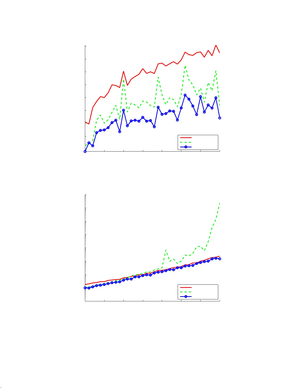
Reduc tion in Sol ving Some In teger Least Squ ares Prob lems Mazen Al Borno Master of Scie nce Sc ho ol of Computer Science McGill Univ ersit y Mon treal, Queb ec F ebruary , 2011 A thesis submitted to Mc G ill Univ ersit y in partial fulﬁlmen t of the requiremen ts of the degree of Master of Scie nce in Computer Scienc e c  Mazen Al Borno 2011 DEDICA TION T o m y lov i n g p ar ents, Manal A b do and A hme d-F ouad A l Borno Go d is the Light of the he avens and the e arth. The Par able of His Light is as if ther e wer e a Niche and within it a L amp: the L amp enclose d in Glass: the gl a s s as it w er e a bril liant star: Lit fr om a blesse d T r e e, an Olive, n either of the e ast nor of the west, whose oi l is wel l-nigh luminous, though ﬁr e sc ar c e touche d it: Light up on Light! Qur’an , 24:35 ii A CKN OWLEDGMENTS I am fortunate to ac kno wledge: • Xiao-W en Chang a s an advisor; for his patience, constructiv e criticism and careful review of this thesis whic h we nt ab ov e and b eyond the call of dut y . • true friends at the Sc ho ol o f Computer Science; I only wish I w as as go o d a friend to y ou, as you to me; Stephen Breen, Z he Chen, Arth ur Guez, Sev a n Hanss ia n, W en-Y ang Ku, M athieu P etitpas, Shao w ei Png, Milena Scaccia, Iv an Sav o v, Ben Spro tt, D a vid Titley-Pe lo quin, Y anc heng Xiao, Xiaoh u Xie, and esp ecially Omar F aw zi; • a wonde rful course on Qua n tum Information Theory by P atric k Hay den; • a younger brother for his limitless generosity and a lo ving family whose the source of m y joy and the remov al of m y sorro w. iii ABSTRACT Solving an in teger least sq uar es (ILS) problem usually consists o f tw o stages: reduction and search. This thesis is concerned with the reduction pro cess for the ordinary ILS problem and the ellipsoid-constrained ILS pro b- lem. F or the ordina r y ILS pro blem, w e disp el common misconceptions on the reduction stage in the literature and sho w what is crucial to the eﬃciency of the searc h pro cess. The new understanding allo ws us to design a new re- duction algorithm which is more eﬃcien t than the w ell-known LLL reduction algorithm. Numerical stabilit y is tak en in to accoun t in designing t he new re- duction algorithm. F or the ellipsoid-constrained ILS problem, w e prop ose a new reduction algorithm whic h, unlik e existing algorithms, uses all the av ail- able info r ma t io n. Sim ulatio n r esults indicate that new algorit hm can greatly reduce the computational cost of the searc h pro cess when the measuremen t noise is larg e. iv ABR ´ EG ´ E La r ´ esolution de probl ` emes de moindres carr ´ es en nom bres en tiers (ILS) comprend habituellemen t deux stages: la r´ e duction et la reche rche. Cette th` es e s’in t ´ eresse ` a la r ´ eduction p our le probl ` eme ILS ordinaire et le probl ` eme ILS sous con trainte d’ellipse. Pour le probl` e me ILS ordinaire, nous dissipo ns des erreurs comm unes de compr ´ ehension ` a prop os de la r´ eduction dans la litt ´ erature et nous mon trons ce qui est r´ eellemen t crucial po ur l’eﬃcacit ´ e de la rec herc he. Ce r ´ esultat nous p ermet de d´ ev elopp er un nouv el algorit hme de r´ eduction plus eﬃ- cace que le c´ el ` ebre algorit hme LLL. La stabilit´ e n um ´ erique est prise en compte dans le d´ ev elopp emen t du nouv el algorithme. P our le pro bl` eme ILS sous con- train te d’ellipse, nous prop osons un nouv el algorit hme de r´ eduction qui, con- trairemen t aux algorithmes existan ts, utilise toute l’informatio n disp o nible. Les r´ esultats de sim ulations indiquen t que le nouv el algorithme r´ eduit con- sid ´ erablement les co ˆ uts de calcul de la reche rche lorsque la v ariance du bruit est la rge dans le mo d ` ele lin ´ eaire. v T ABLE OF CONTE NTS DEDICA TION . . . . . . . . . . . . . . . . . . . . . . . . . . . . . . . ii A CKNO WLEDGMENTS . . . . . . . . . . . . . . . . . . . . . . . . . iii ABSTRA CT . . . . . . . . . . . . . . . . . . . . . . . . . . . . . . . . iv ABR ´ EG ´ E . . . . . . . . . . . . . . . . . . . . . . . . . . . . . . . . . . v LIST O F T ABLES . . . . . . . . . . . . . . . . . . . . . . . . . . . . . viii LIST O F F IGURES . . . . . . . . . . . . . . . . . . . . . . . . . . . . ix LIST O F ABBREVIA TIONS . . . . . . . . . . . . . . . . . . . . . . . 1 1 In tro duction . . . . . . . . . . . . . . . . . . . . . . . . . . . . . . 1 2 The OILS problem in the standard form . . . . . . . . . . . . . . 7 2.1 Search pro cess . . . . . . . . . . . . . . . . . . . . . . . . . 7 2.2 Reduction pro cess . . . . . . . . . . . . . . . . . . . . . . . 11 2.2.1 Intege r G auss t r a nsformations . . . . . . . . . . . . 14 2.2.2 Pe rmutations . . . . . . . . . . . . . . . . . . . . . . 14 2.2.3 LLL reduction . . . . . . . . . . . . . . . . . . . . . 15 3 The OILS problem in the quadratic form . . . . . . . . . . . . . . 18 3.1 Reduction pro cess . . . . . . . . . . . . . . . . . . . . . . . 19 3.1.1 Intege r G auss t r a nsformations . . . . . . . . . . . . 20 3.1.2 Pe rmutations . . . . . . . . . . . . . . . . . . . . . . 21 3.2 LAMBDA reduction . . . . . . . . . . . . . . . . . . . . . 2 3 3.3 MLAMBDA reduction . . . . . . . . . . . . . . . . . . . . 25 3.3.1 Symmetric piv oting strategy . . . . . . . . . . . . . 25 3.3.2 Greedy selection strategy . . . . . . . . . . . . . . . 26 3.3.3 Lazy transformation strategy . . . . . . . . . . . . . 27 3.3.4 The reduction algorithm . . . . . . . . . . . . . . . 2 7 3.4 Search pro cess . . . . . . . . . . . . . . . . . . . . . . . . . 29 4 Reduction Misconceptions and New Reduction Algo rithms . . . . 32 4.1 Impact of decorrelation on the searc h pro cess . . . . . . . . 33 4.1.1 Implications to some reduction strategies . . . . . . 37 vi 4.2 Partial reduction . . . . . . . . . . . . . . . . . . . . . . . 39 4.3 Geometric inte rpretat io n . . . . . . . . . . . . . . . . . . . 43 4.4 A new reduction metho d . . . . . . . . . . . . . . . . . . . 45 4.5 Numerical simu lat io ns . . . . . . . . . . . . . . . . . . . . 50 4.5.1 Setup . . . . . . . . . . . . . . . . . . . . . . . . . . 50 4.5.2 Comparison of the reduction strategies . . . . . . . 52 4.6 Condition num ber criterion . . . . . . . . . . . . . . . . . . 68 4.7 Implications to the standard OILS form . . . . . . . . . . . 70 4.7.1 A partial LLL reduction . . . . . . . . . . . . . . . 7 0 4.7.2 Ling’s and Howgra v e-Graham’s eﬀectiv e LL L reduction 72 5 Ellipsoid-Constrained In teger Least Squares Problems . . . . . . . 73 5.1 Search pro cess . . . . . . . . . . . . . . . . . . . . . . . . . 73 5.2 Reduction . . . . . . . . . . . . . . . . . . . . . . . . . . . 77 5.2.1 A constrain t reduction strategy . . . . . . . . . . . . 77 5.2.2 The ellipsoidal constrain t . . . . . . . . . . . . . . . 80 5.2.3 Computing the b ox-constrain t . . . . . . . . . . . . 81 5.2.4 A new reduction algorithm . . . . . . . . . . . . . . 82 5.3 Numerical simu lat io ns . . . . . . . . . . . . . . . . . . . . 84 5.3.1 Setup . . . . . . . . . . . . . . . . . . . . . . . . . . 85 5.3.2 Comparison of the reduction strategies . . . . . . . 85 6 Summary and future w ork . . . . . . . . . . . . . . . . . . . . . . 91 References . . . . . . . . . . . . . . . . . . . . . . . . . . . . . . . . . . 94 vii LIST OF T ABLES 4–1 Search pro cess without IGT . . . . . . . . . . . . . . . . . . . . 38 4–2 Search pro cess with IGT . . . . . . . . . . . . . . . . . . . . . 38 4–3 Search pro cess with NOREDUCTION . . . . . . . . . . . . . . 42 4–4 Search pro cess with LAMBD A reduction or MREDUCTION . 42 4–5 Search pro cess with MINREDUCTION . . . . . . . . . . . . . 42 4–6 Search pro cess with LAMBD A reduction or MREDUCTION . 49 4–7 Search pro cess with PREDUCTION . . . . . . . . . . . . . . . 5 0 viii LIST OF FIGURES 2–1 A three-dimensional example o f a searc h tree . . . . . . . . . . 10 4–1 Original and transformed searc h space. The tra nsformed search space is less elongat ed. . . . . . . . . . . . . . . . . . . . . 44 4–2 Running time fo r Case 1 . . . . . . . . . . . . . . . . . . . . . 5 5 4–3 Running time fo r Case 2 . . . . . . . . . . . . . . . . . . . . . 5 6 4–4 Running time fo r Case 3 . . . . . . . . . . . . . . . . . . . . . 5 7 4–5 Running time fo r Case 4 . . . . . . . . . . . . . . . . . . . . . 5 8 4–6 Running time fo r Case 5 . . . . . . . . . . . . . . . . . . . . . 5 9 4–7 Running time fo r Case 6 . . . . . . . . . . . . . . . . . . . . . 6 0 4–8 Running time fo r Case 7 . . . . . . . . . . . . . . . . . . . . . 6 1 4–9 Running time fo r Case 8 . . . . . . . . . . . . . . . . . . . . . 6 2 4–10 R unning time for Case 9 . . . . . . . . . . . . . . . . . . . . . 63 4–11 R elat ive bac kw ard error for Case 1 . . . . . . . . . . . . . . . 64 4–12 R elat ive bac kw ard error for Case 2 . . . . . . . . . . . . . . . 64 4–13 R elat ive bac kw ard error for Case 3 . . . . . . . . . . . . . . . 65 4–14 R elat ive bac kw ard error for Case 4 . . . . . . . . . . . . . . . 65 4–15 R elat ive bac kw ard error for Case 5 . . . . . . . . . . . . . . . 66 4–16 R elat ive bac kw ard error for Case 6 . . . . . . . . . . . . . . . 66 4–17 R elat ive bac kw ard error for Case 7 . . . . . . . . . . . . . . . 67 4–18 R elat ive bac kw ard error for Case 8 . . . . . . . . . . . . . . . 67 4–19 R elat ive bac kw ard error for Case 9 . . . . . . . . . . . . . . . 68 5–1 Av erage searc h time v ersus dimension, σ = 0 . 5 . . . . . . . . . . 86 5–2 Av erage searc h time v ersus dimension, σ = 1. . . . . . . . . . . 86 ix 5–3 Av erage searc h time v ersus dimension, σ = 2. . . . . . . . . . . 87 5–4 Av erage searc h time v ersus dimension, σ = 4. . . . . . . . . . . 87 5–5 Av erage searc h time v ersus dimension, σ = 10 . . . . . . . . . . 88 5–6 Ratio b et w een β at the Babai in teger p oint and β at the EILS solution, dimension n = 5. . . . . . . . . . . . . . . . . . . . 88 x CHAPTER 1 In tro duction Supp ose w e hav e the following linear mo del y = Ax + v , (1.1) where y ∈ R m is a me asur e m ent ve ctor , A ∈ R m × n is a design m atrix with full column ra nk, x ∈ R n is an unkno wn p ar ameter ve ctor , and v ∈ R n is a noise ve ctor that follows a normal distribution with mean 0 and co v ariance σ 2 I . W e need to ﬁnd an estimate ˆ x of the unkno wn v ector x . One approa ch is to solv e the fo llo wing r e al le ast squar es (LS) problem min x ∈ R n k y − Ax k 2 2 . (1.2) W e refer to (1 .2) as the standard form of the LS problem. The real least squares solution is given by (see, e.g., [20, Section 5.3]) ˆ x = ( A T A ) − 1 A T y . (1.3) Substituting (1.1 ) into (1 .3), w e get ˆ x = x + ( A T A ) − 1 A T v . (1.4) Let W ˆ x ∈ R n × n b e the cov ariance matrix of ˆ x . Using the la w of co v ariance propagation on (1.4) (see, e.g., [33, p. 329]), it follo ws that W ˆ x = σ 2 ( A T A ) − 1 . In man y applications, x is constrained to some discrete in teger set D , e.g., a b o x constrain t. Then, one w ants to solv e the inte ger le ast squar es (I LS ) 1 pr oblem min x ∈D k y − Ax k 2 2 . (1.5) If D is the whole in tegral space Z n , then we refer to min x ∈ Z n k y − Ax k 2 2 (1.6) as t he or dinary inte ger le ast sq uar es (OILS) pr oblem . In lattice theory , the set L ( A ) = { Ax : x ∈ Z n } is referred to as the lattice generated by A . The OILS problem is to ﬁnd the p oin t in L ( A ) whic h is closest to y . F o r this r eason, the OILS problem is also called the closest p oint pr o b lem . Since the residual y − A ˆ x is ortho g onal to the range of A , w e hav e k y − Ax k 2 2 = k y − A ˆ x − A ( x − ˆ x ) k 2 2 = k y − A ˆ x k 2 2 + k A ( x − ˆ x ) k 2 2 = k y − A ˆ x k 2 2 + ( x − ˆ x ) T A T A ( x − ˆ x ) = k y − A ˆ x k 2 2 + σ 2 ( x − ˆ x ) T W − 1 ˆ x ( x − ˆ x ) . (1.7) Th us, the OILS problem (1.6) is equiv alen t to min x ∈ Z n ( x − ˆ x ) T W − 1 ˆ x ( x − ˆ x ) . (1.8) W e refer to (1.8) as the quadratic form of the OILS problem. ILS problems ar ise from man y applications, suc h as global na vigation satellite system s, comm unications, bioinformatics, radar imaging, cryptogra- ph y , Mon te Carlo second-momen t estimation, lattice design, etc., see, e.g., [1] and [22]. Unlike the real least squares problem (1.2), the ILS problem (1.5) is NP-hard (see [4] and [29]). Since a ll known alg o rithms to solv e the ILS prob- lem hav e exp o nen tial complexity , designing eﬃcien t alg orithms is crucial for real-time applications. A ty pical a pproac h for solving an ILS problem consists of t wo stages: reduction and searc h. The reduction pro cess tra nsfor ms (1.5) to a new ILS problem, where A is reduced to an upp er triangular matrix. The searc h pro cess searc hes fo r the solution of the new ILS problem in a geometric 2 region. The main goal of the reduction pro cess is to mak e the searc h pro cess more eﬃcien t. F or solving (1.6), t w o t ypical reduction strategies are emplo y ed in practice. One is the Korkine-Zolotareﬀ (KZ) reduction (see [24]), whic h transforms the original OILS problem to a new one whic h is o ptimal for the searc h pro cess. The o ther is the Lenstra-Lenstra-Lov ´ asz (LLL) reduction (see [25]), whic h transforms t he original OILS problem to a new one whic h is approx imately optimal for the searc h pro cess. Unlike the KZ r eduction, it is kno wn ho w to compute the LLL reduction eﬃcien tly in p olynomial time. F or t his reason, the LLL reduction is more widely used in practice. Sim ulations in [1] suggest to use the KZ reduction only if w e hav e to solv e man y OILS problems with the same g enerato r matrix A . Otherwise, the LLL reduction should b e used. F or the searc h pro cess, t wo common searc h strategies are the P ohst enum eratio n strategy (see [1 8]) and the Sc hnorr-Euchn er en umeration strategy (see [32]). Both examine the lattice p oints lying inside a hyper-sphere, but in a diﬀeren t order. Sim ulations in [1] indicate that the Schnorr-Euc hner strategy is mo r e eﬃcien t than the P ohst strategy . In high precision relativ e g lobal nav igat io n satellite systems (GNSS) p osi- tioning, a k ey comp onent is to resolv e the unkno wn so-called double diﬀerenced cycle ambiguities of the carrier phase data a s in tegers. The most success- ful metho d of ambiguit y resolution in the GNSS literature is the w ell-kno wn LAMBD A (Least-squares AMBiguity Decorrelation Adjustmen t) metho d pre- sen ted b y T eunissen (see, e.g., [34, 35, 36, 38, 3 9]). This metho d solves the OILS problem (1.8). A detailed description of t he LAMBD A algorithm and implemen tation is g iven by [16]. Its softw are (F ortran ve rsion and MA TLAB v ersion) is av ailable from Delft Univ ersit y of T ec hnology . F requen tly a sk ed questions and misunderstanding ab out the LAMBD A metho d are addressed b y [17]. Recen tly , a mo diﬁed metho d called MLAMBD A w as prop o sed b y 3 Chang etc in [10], whic h w as then further mo diﬁed and extended to han- dle mixed ILS problems b y using orthogo nal t ransformations, resulting in t he MA TLAB pack age MILS (see [12]). In some applications, the p oint A x in (1.5) is constrained to b e inside a giv en hy p er-sphere. The ILS problem b ecomes min x ∈E k y − Ax k 2 2 , E = { x ∈ Z n : k Ax k 2 2 ≤ α 2 } , (1.9) see [9] and [15]. W e refer to (1.9) as the el lipsoid-c onstr aine d inte ger le ast squar es (EILS) pr oblem . T o solv e the EILS problem, [9] prop osed the LLL reduction in the reduction stage and mo diﬁed the Schnorr-Euc hner searc h strategy to handle the ellipsoidal constraint in the searc h stag e. The con tribution of this thesis is t w o-f old. The ﬁrst is to disp el com- mon misconceptions on the reduction pro cess app earing in the ILS literature. The second is to presen t more eﬃcien t algorithms to solv e the ILS and EILS problem. The thesis is orga nized a s follows. In Chapter 2, w e review the t ypical metho ds to solv e an OILS problem. Sp eciﬁcally , we in tro duce the LLL reduction metho d and the Schnorr-Euc hner searc h strategy . In Chapter 3, w e discuss t he t ypical metho ds to solv e the quadratic for m of the OILS problem. Our fo cus will b e on LAMBD A reduction a nd the mo diﬁed reduction (MREDUCTION) giv en in [10]. According to the literature, there are t wo goals the reduction pro cess should ac hiev e to mak e the searc h pro cess eﬃcien t. One of them is to trans- form the generator matrix A in (1.6) or the co v ariance matrix W ˆ x in (1.8) t o a mat r ix whic h is as close to diagonal as p ossible. A cov ariance matrix whic h is close to dia gonal means that there is little correlat io n b et we en its random v ariables. In other w ords, the goal of the reduction in the GNSS context is to decorrelate the am biguities as muc h as p ossible. T o ac hiev e this g oal, the reduction pro cess uses so-called inte ger Gauss tr ansformations. In Chapter 4, w e sho w that, con tra ry to common b elief, this g oal will not mak e t he search 4 more eﬃcien t. W e pro vide a new explanation on the role of integer Gauss transformations in the reduction pro cess. This new understanding results in mo diﬁcations to the existing reduction metho ds. Numerical sim ulations indi- cate that our new algorithms are more eﬃcien t than the existing algo rithms. Finally , w e discuss another misconception in some GNSS lit erature where it is b eliev ed that the reduction pro cess should reduce the condition num b er of the cov ariance matrix. W e prov ide examples that show that this g oal should b e discarded. In Chapter 5, w e discuss the EILS problem. One drawbac k with the existing reduction algor it hms is t hat the searc h time b ecomes more and more prohibitiv e as the noise v in (1.1) g ets larger. W e presen t a new reduction algorithm whic h, unlik e the LLL reduction, uses the information of the input v ector y and the ellipsoidal constrain t. Then, w e provide simulations tha t sho w that our pro p osed approac h greatly impro v es the searc h pro cess for large noise. Finally , w e summarize our results and men tion our future w ork in Chapter 6. W e now describ e the notation used in this thesis. The sets of all real and in teger m × n matrices are denoted by R m × n and Z m × n , resp ectiv ely , and the set of real and in teger n -v ectors a re denoted b y R n and Z n , resp ectiv ely . Bold upp er case letters and b old lo w er case letters denote matrices a nd v ectors, resp ectiv ely . The iden tit y matrix is denoted b y I and its i th column is denoted b y e i . Sup erscript T denotes the transp ose. The 2- norm of a v ector o r a matrix is denoted by k · k 2 . MA TLAB not ation is used to denote a submatrix. Sp eciﬁcally , if A = ( a ij ) ∈ R m × n , then A ( i, :) denotes the i th ro w, A (: , j ) the j th column, and A ( i 1 : i 2 , j 1 : j 2 ) the submatrix formed b y r ows i 1 to i 2 and columns j 1 to j 2 . F or the ( i, j ) elemen t of A , w e denote it by a ij or A ( i, j ). F or the i th en try of a ve ctor a , we denote it b y a i . F or a scalar z ∈ R , w e use ⌊ z ⌉ to denote its nearest integer. If there is a tie, ⌊ z ⌉ denotes the one with smaller magnitude. The op eration sign(z) returns − 1 if z ≤ 0 a nd 1 if 5 z > 0. F o r a random v ector x ∈ R n , x ∼ N (0 , σ 2 I ) means that x follow s a normal distribution with mean 0 and cov ariance matrix σ 2 I . W e use i.i.d. to abbreviate “independently and iden tically distributed”. 6 CHAPTER 2 The OILS problem in the standard form The OILS problem is deﬁned as min x ∈ Z n k y − Ax k 2 2 , ( 2 .1) where y ∈ R n and A ∈ R m × n has full column rank. In this c hapter, w e review the typ ical metho ds to solv e the OILS problem. A t ypical approach for solving an OILS problem consists of tw o stages: reduction and search. The main g o al of the reduction pro cess is to mak e the searc h pro cess eﬃcien t. In order to b etter understand the aims of the reduction, w e ﬁrst introduce the searc h pro cess and the Schnorr-Euc hner searc h strategy in Section 2 .1 . Then, w e presen t the reduction pro cess and the w ell-known LLL reduction in Section 2.2. 2.1 Searc h pro cess Supp ose that after the reduction stage, the O ILS problem (2.1) is transformed to min z ∈ Z n k ¯ y − Rz k 2 2 , (2.2) where R ∈ R n × n is nonsingular upp er triangular and ¯ y ∈ R n . Assume that the solution of (2.2 ) satisﬁes the b ound k ¯ y − Rz k 2 2 < β 2 , 7 or equiv alen tly n X k =1 ( ¯ y k − n X j = k +1 r k j z j − r k k z k ) 2 < β 2 . (2.3) Since (2.3) is a h yp er-ellipsoid, w e refer to it as a searc h ellipsoid. The goal of the searc h pro cess is to ﬁnd an integer p oin t inside the search ellipsoid whic h minimizes the left-hand side of ( 2 .3). Let c n = ¯ y n /r nn , c k = ( ¯ y k − n X j = k +1 r k j z j ) /r k k , k = n − 1 : − 1 : 1 . (2.4) Note that c k dep ends on z k +1 , . . . , z n . Substituting ( 2.4) in (2.3), we hav e n X k =1 r 2 k k ( z k − c k ) 2 < β 2 . (2.5) If z satisﬁes the b ound, then it mus t also satisfy inequalities lev el n : r 2 nn ( z n − c n ) 2 < β 2 , (2.6) . . . lev el k : r 2 k k ( z k − c k ) 2 < β 2 − n X i = k +1 r 2 ii ( z i − c i ) 2 (2.7) . . . lev el 1 : r 2 11 ( z 1 − c 1 ) 2 < β 2 − n X i =2 r 2 ii ( z i − c i ) 2 . (2.8) The searc h pro cess starts at lev el n and mov es down to lev el 1. At lev el k , z k is determined for k = n : − 1 : 1. F rom (2.7), the range of z k is [ l k , u k ], where l k = l c k − ( β 2 − n X i = k +1 r 2 ii ( z i − c i ) 2 ) 1 / 2 / | r k k | m and u k = j c k + ( β 2 − n X i = k +1 r 2 ii ( z i − c i ) 2 ) 1 / 2 / | r k k | k . 8 There are tw o t ypical strategies to examine the in tegers inside [ l k , u k ]. In the P ohst strategy (see [1 8]), the in tegers are c hosen in the ascending order l k , l k + 1 , l k + 2 , . . . , u k . In the Schnorr-Euc hner strategy (see [32]), the in tegers are chos en in the zig- zag o r der z k =      ⌊ c k ⌉ , ⌊ c k ⌉ − 1 , ⌊ c k ⌉ + 1 , ⌊ c k ⌉ − 2 , . . . , if c k ≤ ⌊ c k ⌉ ⌊ c k ⌉ , ⌊ c k ⌉ + 1 , ⌊ c k ⌉ − 1 , ⌊ c k ⌉ + 2 , . . . , if c k ≥ ⌊ c k ⌉ . (2.9) Observ e t ha t in Sc hnorr-Euc hner strategy , once an in teger z k do es not satisfy (2.7), all the follow ing in tegers in the sequence will not satisfy it. These in tegers can b e pruned from the se ar ch pro cess. Suc h a prop ert y do es not exist in t he P ohst strategy . Another b eneﬁt with t he Sc hnorr-Euc hner en umeration order is that the ﬁrst p oin ts examined a re more lik ely to minimize (2.5) tha n the la st p oints examined. As will b e seen in the next parag raph, this allow s to shrink the searc h ellipsoid faster. Sim ulations in [1] conﬁrm tha t t he Sc hnorr- Euc hner strategy is more eﬃcien t than the P ohst strategy . W e now describe the searc h pro cess using the Sc hnorr-Euc hner strat egy . A t lev el n , w e compute c n b y (2.4) and set z n = ⌊ c n ⌉ . If (2.6) is not satisﬁed, no in teger can satisfy (2.5). Otherwise, w e go to lev el n − 1, compute c n − 1 and set z n − 1 = ⌊ c n − 1 ⌉ . If (2.7) do es not hold, we go back to leve l n and c ho ose z n to b e the second nearest integer to c n . Otherwise, w e mo v e down to lev el n − 2. When w e reach lev el 1, we compute c 1 and set z 1 = ⌊ c 1 ⌉ . Then, if (2.8) is satisﬁed, w e set ˆ z = [ z 1 , . . . , z n ] T , where ˆ z is a full integer p oint inside the searc h ellipsoid. W e up date β b y setting β 2 = P n k =1 r 2 k k ( ˆ z k − c k ) 2 . This step allo ws to eliminate more p oin ts b y “shrinking” the searc h ellipsoid. Now w e searc h for a b etter p oint than ˆ z . If one is found, w e up dat e ˆ z . W e mo v e up 9 Figure 2–1: A three-dimensional example of a searc h tree to lev el 2 and c ho ose z 2 to b e the next nearest inte ger to c 2 , where “next” is relativ e to ˆ z 2 . If inequalit y (2.7) holds at leve l 2, we mo ve do wn to leve l 1 and up date z 1 ; otherwise, w e mov e up to lev el 3 and up date z 3 . The pro cedure con tin ues un til w e reac h lev el n and ( 2 .6) is not satisﬁed. The last full intege r p oint found is the OILS solution. The describ ed searc h pro cess is a depth-ﬁrst searc h, see a n example of a search tree in Fig. 2– 1 . T he ro ot no de do es not corresp ond to an elemen t in z , but is used to unite the bra nc hes into a tree. Note that the in tegers are en umerated according to order (2.9) when we mov e up one lev el in the searc h. If the initial v alue of β is ∞ , the ﬁrst integer p oint found is called the Babai in teger p oin t. W e describ e the pro cess as an algorithm, see [7]. Algorithm 2.1.1. (SEAR CH) Giv en nonsingular upp er triangular matrix R ∈ R n × n and ¯ y ∈ R n . The Sc hnorr- Euc hner searc h alg o rithm ﬁnds the optimal solution to min z ∈ Z n k ¯ y − Rz k 2 2 . function : z = SEAR CH( R , ¯ y ) 1. (Initializat io n) Set k = n, β = ∞ . 2. Compute c k from ( 2 .4). Set z k = ⌊ c k ⌉ , ∆ k = sgn( c k − z k ) 3. (Main step) 10 if r 2 k k ( z k − c k ) 2 > β 2 − P n i = k +1 r 2 ii ( z i − c i ) 2 go to Step 4 else if k > 1 k = k − 1, go to Step 2 else // case k = 1 go to Step 5 end 4. (Inv alid p oin t) if k = n terminate else k = k + 1, g o t o Step 6 end 5. (F o und v alid p oin t) Set ˆ z = z , β 2 = P n k =1 r 2 k k ( ˆ z k − c k ) 2 k = k + 1, g o t o Step 6 6. (Enume ra t io n at lev el k) Set z k = z k + ∆ k , ∆ k = − ∆ k − sgn (∆ k ) go to Step 3 . 2.2 Reduction pro cess In the reduction pro cess, we transform A to an upp er tr ia ngular matr ix R whic h has prop erties that mak e the searc h pro cess more eﬃcien t. Since (2.1) uses the 2-norm, w e can a pply an orthogo nal transformation Q T to the left of A as long as it is also applied to the left of y , i.e., k y − Ax k 2 2 = k Q T y − Q T Ax k 2 2 . In order to main tain the in teger nature of x , the transformation Z applied to the right of A mus t b e an in teger matrix, whose in ve rse is also 11 an inte ger matr ix. It is easy to v erify that | det( Z ) | = 1, as b ot h det( Z ) and det( Z − 1 ) are integers, and det( Z )det( Z − 1 ) = 1. Suc h in teger matrices a re referred to as unimo dular mat r ices. The tr a nsformations o n A can b e describ ed as a QRZ f a ctorization of A : Q T AZ =    R 0    or A = Q T 1 RZ − 1 , (2.10) where Q = [ Q 1 , Q 2 ] ∈ R m × m is o rthogonal, R ∈ R n is no nsingular upp er triangular and Z ∈ Z n × n is unimo dular (see [9]). Using this f a ctorization, k y − Ax k 2 2 = k Q T 1 y − RZ − 1 x k 2 2 + k Q T 2 y k 2 2 . (2.11) Let ¯ y = Q T 1 y , z = Z − 1 x . (2.12) Then, w e can rewrite (2.1) as min z ∈ Z n k ¯ y − Rz k 2 2 . (2.13) If ˆ z is the solution of the transformed OILS problem (2.13), t hen ˆ x = Z ˆ z is the solution of the original OILS problem (2.1). Note that R in (2 .1 0) is no t unique. A diﬀeren t Z usually leads to a diﬀeren t R . Without loss of generality , we assume that the diagonal en tries of R are p ositiv e in this thesis. Certain prop erties of R can mak e the searc h pro cess m uc h more eﬃcien t. If R is diagonal, then simply rounding all c k to the nearest in teger giv es the optimal solution. In [30], it is claimed that as R gets closer to a diagonal matrix, the complexit y of the search pro cess decreases. In Section 4.1, w e sho w that this claim is not true. The crucial prop ert y that R m ust strive for is that r k k should b e as large as p ossible for large k . W e motiv ate this prop erty by a t wo dimensional case ( n = 2). Let r 22 ≪ r 11 . 12 In the searc h pro cess, the b ound (2.6) a t lev el 2 is very lo ose, implying that there are many v alid in tegers z 2 . How ev er, the b o und (2 .8 ) at lev el 1 is v ery tigh t. Hence, aft er z 2 is ﬁxed, there is a high probabilit y that no v alid inte ger z 1 exists. W e m ust en umerate man y integers at lev el 2 b efore w e can ﬁnd a v alid integer at lev el 1. This is the so-called search halting pro blem (see [3 6]). Note that det( A T A ) = det( R T R ) = r 2 11 . . . r 2 nn is constan t, indep enden t of the c hoice of Z . Making r k k as large as p o ssible for large k implies making r k k as small as p o ssible for small k . Hence, w e can say that the reduction pro cess should striv e for r 11 ≪ . . . ≪ r nn . (2.14) The t ypical r eduction metho d for the OILS problem is the LL L reduction (see [25] and [22]). The LLL reduction can b e written in the form of a QRZ factorization, where R satisﬁes the following criteria | r k − 1 ,j | ≤ 1 2 r k − 1 ,k − 1 , j = k , . . . , n (2.15) r k − 1 ,k − 1 ≤ δ q r 2 k − 1 ,k + r 2 k k , 1 ≤ δ < 2 and k = 2 , . . . , n. (2.16) Notice that ta king δ = 1 is b est to striv e f or (2.14). In this thesis, w e alw a ys tak e δ = 1 . The LLL r eduction cannot guaran tee r 11 ≤ . . . ≤ r nn , but substituting (2.15) in to (2.16), w e see that it can guaran tee r k − 1 ,k − 1 ≤ 2 √ 3 r k k , k = 2 , . . . , n. In our implemen tation of the LLL reduction, w e use tw o ty p es of unimo d- ular transformations to ensure prop erties (2.15) and (2.16). These are integer Gauss transformations and p erm utation matrices. In the fo llowing, w e presen t the eﬀect of t hese transformations on the R factor o f t he QR fa ctorization of A . 13 2.2.1 In teger Gauss transformations Supp ose we ar e giv en an upp er triangula r matrix R with p ositiv e diagonal en tries. An in teger Gauss transformation (IGT) Z ij has the f o llo wing form Z ij = I − µ e i e T j , µ is an in teger . (2.17) Applying Z ij ( i < j ) to R from the r igh t give s ¯ R = RZ ij = R − µ Re i e T j . Th us ¯ R is the same as R , except that ¯ r k j = r k j − µr k i , k = 1 , . . . , i. T a king µ = ⌊ r ij /r ii ⌉ ensures that | ¯ r ij | ≤ 1 2 r ii . Similarly , an IGT Z ij ( i > j ) can b e a pplied to a unit lo wer triangular matrix L from the right t o ensure that | ¯ l ij | ≤ 1 / 2. 2.2.2 P erm utations F or R to satisfy (2.16) with δ = 1, w e sometimes need to p erm ute its columns. In the reduction pro cess, if r k − 1 ,k − 1 > q r 2 k − 1 ,k + r 2 k k , w e p erm ute columns k and k − 1. RP k − 1 ,k =       R 11 ¯ R 12 R 13 ˜ R 22 R 23 R 33       , where P k − 1 ,k =       I k − 2 P I n − k       , P =    0 1 1 0    , ˜ R 22 =    r k − 1 ,k r k − 1 ,k − 1 r k k 0    , 14 ¯ R 12 = [ R (1 : k − 2 , k − 1) , R (1 : k − 2 , k )] . As a result, R is no longer upp er triang ular. T o mak e it upp er triangular again, w e apply a G iv ens rotation G to zero elemen t r k k in ˜ R 22 . G ˜ R 22 = ¯ R 22 , or    c s − s c       r k − 1 ,k r k − 1 ,k − 1 r k k 0    =    ¯ r k − 1 ,k − 1 ¯ r k − 1 ,k 0 ¯ r k k    , where ¯ r k − 1 ,k − 1 = q r 2 k − 1 ,k + r 2 k k , c = r k − 1 ,k ¯ r k − 1 ,k − 1 , s = r k k ¯ r k − 1 ,k − 1 (2.18) ¯ r k − 1 ,k = cr k − 1 ,k − 1 , ¯ r k k = − sr k − 1 ,k − 1 . (2.19) Therefore, w e ha v e Q k − 1 ,k RP k − 1 ,k = ¯ R =       R 11 ¯ R 12 R 13 ¯ R 22 ¯ R 23 R 33       , Q k − 1 ,k =       I k − 2 G I n − k       , ¯ R 23 = GR 23 . After the p erm utation, inequalit y ¯ r k − 1 ,k − 1 ≤ q ¯ r 2 k − 1 ,k + ¯ r 2 k k no w holds. While a p erm utation do es not g uaran tee ¯ r k − 1 ,k − 1 ≤ ¯ r k k , it do es guaran tee that ¯ r k − 1 ,k − 1 < r k − 1 ,k − 1 and ¯ r k k > r k k . Suc h a p erm utation is useful since the diagonal elemen ts of R are no w closer to ( 2 .14). 2.2.3 LLL reduction The LLL reduction algorithm give n in [9] starts by ﬁnding the QR decomp o- sition of A b y Householder transforma t io ns, then computes ¯ y and works with 15 R from left to righ t. At the k th column of R , the alg orithm applies IGTs to ensure that | r ik | < 1 2 r ii for i = k − 1 : − 1 : 1. Then, if inequalit y (2.16) holds, it mo ves to column k + 1; otherwise it p erm utes columns k and k − 1, applies a Give ns rotation to R fr o m the left to bring R bac k to a n upp er tr ia ngular form, sim ultaneously applies the same G ivens ro tation to ¯ y , a nd mo ve s to col- umn k − 1. W e describe our implemen tation of the LLL reduction as follow s (see [9]). Algorithm 2.2.1. (LLL Reduction). Giv en the generator matrix A ∈ R m × n and the input v ector y ∈ R m . The algorit hm returns the reduced upp er triangular matrix R ∈ R n × n , the unimo dular matrix Z ∈ Z n × n , and the v ector ¯ y ∈ R n . function : [ R , Z , ¯ y ] = LLL( A , y ) Compute QR factorization o f A and set ¯ y = Q T 1 y Z = I k = 2 while k ≤ n for i = k − 1 : − 1 : 1 Apply IG T Z ik to R , .i.e., R = R Z ik Up date Z , i.e., Z = Z Z ik end if r k − 1 ,k − 1 > q r 2 k − 1 ,k + r 2 k k In terc hange columns k and k − 1 of R a nd Z T r a nsform R to a n upp er triangular matrix b y a Giv ens rotation Apply the same Givens rota tion t o ¯ y if k > 2 k = k − 1 end 16 else k = k + 1 end end 17 CHAPTER 3 The OILS problem in the quadratic form A prerequisite for high precision relative GNSS p ositioning is to resolv e the unkno wn double diﬀerenced cycle ambiguities of the carrier phase data as in tegers. This turns out to b e an OILS problem. Supp ose ˆ x ∈ R n is t he real-v alued least squares estimate of the in teger parameter ve ctor x ∈ Z n (i.e., the double diﬀerenced integer ambiguit y v ector in the GNSS context) and W ˆ x ∈ R n × n is it s co v ariance matrix, whic h is symmetric p ositiv e deﬁnite. The OILS estimate ˇ x is the solution of the minimization problem: min x ∈ Z n ( x − ˆ x ) T W − 1 ˆ x ( x − ˆ x ) . (3.1) Although (3.1) is in the form of a n integer quadratic optimization prob- lem, it is easy to rewrite it in the standard OILS for m (2 .1). W e refer to (3.1) as the quadratic form of the OILS problem. In Section 3.1, w e discuss the reduction pro cess used in the GNSS literature. In Section 3.2, w e review the reduction stage in the LAMBDA (Least-squares AMBiguit y Decorrelation Adjustmen t) metho d (e.g., [3 4, 35, 36, 38, 39]). In Section 3.3, w e in tro duce the impro ve ments to the reduction pro vided b y t he MLAMBD A (Mo diﬁed LAMBD A) metho d (see [10]). Finally in Section 3 .4, w e brieﬂy review the searc h pro cess in the quadratic form of the OILS pro blem. 18 3.1 Reduction pro cess The reduction step uses a unimo dular matrix Z to transform (3.1) in to min z ∈ Z n ( z − ˆ z ) T W − 1 ˆ z ( z − ˆ z ) , (3.2) where z = Z T x , ˆ z = Z T ˆ x and W ˆ z = Z T W ˆ x Z . If ˇ z is the in teger minimizer of (3.2), t hen ˇ x = Z − T ˇ z is the in teger minimizer of (3 .1). The b eneﬁt of the reduction step is that the searc h in the new optimization problem (3.2) can b e muc h more eﬃcien t. If W ˆ z is a diagonal matrix, then the transformed am biguities z 1 , . . . , z n are uncorrelated to eac h other. In t his case, simply setting z i = ⌊ ˆ z i ⌉ , for i = 1 : n , w ould minimize t he ob jectiv e function. Let the L T D L factorizatio n of W ˆ z b e W ˆ z = L T D L , (3.3) where L is unit low er triangular and D = diag( d 1 , . . . , d n ) with d i > 0. These factors ha ve a statistical in terpretation. Let ¯ z i denote t he least- squares es- timate of z i when z i +1 , . . . , z n are ﬁxed. As show n in [38, p. 337], d i is the v ariance o f ¯ z i , which is denoted b y σ 2 ¯ z i . F urthermore, l ij = σ ˆ z i ¯ z j σ − 2 ¯ z j for i > j , where σ ˆ z i ¯ z j denotes the co v ariance b et w een ˆ z i and ¯ z j . In the literature (see, e.g., [16], [33, p. 4 98] and [3 8, p. 369]), it is often men tionned that the follow ing tw o goals should b e pursued in t he reduction pro cess b ecause they are crucial for the eﬃciency of the searc h pro cess: (i) W ˆ z is as diagonal as possible. F rom (3.3), for i 6 = j , making L ( i + 1 : n, i ) and L ( j + 1 : n, j ) closer t o 0 mak es W ˆ z ( i, j ) closer to 0. Hence, making the absolute v alues of the oﬀ-diagonal en tries of L a s small as p o ssible mak es W ˆ z as diagonal as p ossible. A co v ariance matrix which is close to diagona l means tha t there is little cor r elation b et w een its random 19 v ariables. In o ther w ords, the goal of the reduction is to decorrelate the am biguities as m uch as p ossible. (ii) The diagonal en tries of D are distributed in decreasing order if p ossible, i.e., one strives for d 1 ≫ d 2 ≫ · · · ≫ d n . (3.4) Note t hat w e wan t d 1 to b e as lar g e as p ossible and d n to b e as small as p ossible. W e can sho w that striving fo r (3.4) is equiv alent to striving for (2.14), where d i corresp onds to r − 2 ii for i = 1 : n . In the reduction pro cess of the LAMBD A metho d, the unimo dular matrix Z is constructed b y a sequenc e of in teger Gauss transformations and permutations. The reduction pro cess starts with the L T DL factor izat io n of W ˆ x and up dates the f actors to g iv e t he L T DL factorization of W ˆ z . The main con tribution of this thesis is to sho w that, con trary to common b elief, the ﬁrst goal will no t mak e the searc h pro cess more eﬃcien t. While lo we r tria ng ula r in teger Ga uss transformations are used to mak e the absolute v alues of the oﬀ-diagonal en tries of L as small as possible, w e argue that they are useful b ecause they help achiev e the second goal. In [26], [27] a nd [43], instead of (i) and (ii), the condition num ber of W ˆ z is used to ev aluate the reduction pro cess. In Section 4.6, we sho w that this criterion can b e misleading and that it is not as eﬀectiv e as (ii). 3.1.1 In teger Gauss transformations In teger Gauss transformations (IGTs) were ﬁrst in tro duced in Section 2.2.1. W e apply Z ij with µ = ⌊ l ij ⌉ (see (2.17)) to L from the righ t, i.e., ¯ L = LZ ij , to ma ke | ¯ l ij | a s small as p ossible. This ensures that | ¯ l ij | ≤ 1 / 2 , i > j. (3.5) 20 W e use the fo llowing algorit hm to apply the IGT Z ij to transform the OILS problem (see [10]). Algorithm 3.1.1. (Inte ger Gauss T ransformations). Giv en a unit low er tri- angular L ∈ R n × n , index pair ( i, j ), ˆ x ∈ R n and Z ∈ Z n × n . This algorit hm applies the in teger G auss tr ansformation Z ij to L suc h that | ( LZ )( i, j ) | ≤ 1 / 2, then computes Z T ij ˆ x a nd Z Z ij , whic h o verw rite ˆ x a nd Z , resp ectiv ely . function : [ L , ˆ x , Z ] = GAUSS( L , i, j, ˆ x , Z ) µ = ⌊ L ( i, j ) ⌉ if µ 6 = 0 L ( i : n, j ) = L ( i : n, j ) − µ L ( i : n, i ) Z (1 : n, j ) = Z (1 : n, j ) − µ Z (1 : n, i ) ˆ x ( j ) = ˆ x ( j ) − µ ˆ x ( i ) end 3.1.2 P erm utations In order t o striv e fo r order (3.4), symmetric p erm utations o f the co v ariance matrix W ˆ x are needed in the reduction. After a p erm utation, the factors L and D of the L T DL factorization ha v e to b e up dated. If we partitio n the L T DL factorization of W ˆ x as follo ws W ˆ x = L T D L =       L T 11 L T 21 L T 31 L T 22 L T 32 L T 33             D 1 D 2 D 3             L 11 L 21 L 22 L 31 L 32 L 33       k − 1 2 n − k − 1 k − 1 2 n − k − 1 . Let P =    0 1 1 0    , P k ,k +1 =       I k − 1 P I n − k − 1       . 21 It can b e show n that P T k ,k +1 W ˆ x P k ,k +1 has the L T DL factorization P T k ,k +1 W ˆ x P k ,k +1 =       L T 11 ¯ L T 21 L T 31 ¯ L T 22 ¯ L T 32 L T 33             D 1 ¯ D 2 D 3             L 11 ¯ L 21 ¯ L 22 L 31 ¯ L 32 L 33       , (3.6) where ¯ D 2 =    ¯ d k ¯ d k +1    , ¯ d k +1 = d k + l 2 k +1 ,k d k +1 , ¯ d k = d k ¯ d k +1 d k +1 , (3.7) ¯ L 22 ≡    1 ¯ l k +1 ,k 1    , ¯ l k +1 ,k = d k +1 l k +1 ,k ¯ d k +1 , (3.8) ¯ L 21 =    − l k +1 ,k 1 d k ¯ d k +1 ¯ l k +1 ,k    L 21 =    − l k +1 ,k 1 d k ¯ d k +1 ¯ l k +1 ,k    L ( k : k + 1 , 1 : k − 1 ) , ( 3 .9) ¯ L 32 = L 32 P =  L ( k + 2 : n, k + 1) L ( k + 2 : n, 1 : k )  . (3.10) W e r efer to such an op eration a s a p ermutation b et we en pair ( k , k + 1). W e describe the pro cess as an algo rithm (see [10 ]) . Algorithm 3.1.2. (P erm utations). Giv en the L and D factors of the L T DL factorization of W ˆ x ∈ R n × n , index k , scalar δ whic h is equal to ¯ d k +1 in (3.7), ˆ x ∈ R n , and Z ∈ Z n × n . This algorithm computes the up da t ed L and D factors in (3.6) after W ˆ x ’s k th row and ( k + 1)th row, a nd k th column and ( k + 1)th column a r e interc hanged, resp ectiv ely . It also in terc hanges ˆ x ’s k th en try and ( k + 1)th en try and Z ’s k th column and ( k + 1 )th column. function : [ L , D , ˆ x , Z ] = PERMUTE( L , D , k , δ, ˆ x , Z ) η = D ( k , k ) /δ // see (3.7) λ = D ( k + 1 , k + 1) L ( k + 1 , k ) / δ // see (3.8) D ( k , k ) = η D ( k + 1 , k + 1) // see (3 .7) 22 D ( k + 1 , k + 1) = δ L ( k : k + 1 , 1 : k − 1 ) =    − L ( k + 1 , k ) 1 η λ    L ( k : k + 1 , 1 : k − 1) // see (3.9) L ( k + 1 , k ) = λ sw ap columns L ( k + 2 : n, k ) and L ( k + 2 : n, k + 1) // see (3 .1 0) sw ap columns Z (1 : n, k ) and Z (1 : n, k + 1) sw ap en tries ˆ x ( k ) and ˆ x ( k + 1) 3.2 LAMBD A reduction W e now describ e the reduction pro cess of the LAMBDA metho d ( see [16, Sect. 3]). F ir st, it computes the L T DL factorization of W ˆ x . The algor it hm starts with column n − 1 of L . A t column k , IGTs ar e applied to ensure that the absolute v alues of the entries b elo w the ( k , k )th en try are as small as p ossible. Then, if ¯ d k +1 ≥ d k +1 holds (see (3.7) ), it mov es to column k − 1; otherwise it p ermu tes pair ( k , k + 1) and mov es bac k to the initial p o sition k = n − 1. The algorit hm uses a v ariable ( k 1 in Algorithm 3.2.1 b elow) to trac k down the columns whose oﬀ- diagonal en tries in magnitude a re already b ounded ab ov e by 1/2 due to previous in teger Gauss transformations. W e presen t the implemen tation giv en in [10]. Algorithm 3.2.1. (LAMBD A REDUCTION). Given the cov ariance matr ix W ˆ x and real- v alued LS estimate ˆ x o f x . This alg orithm computes an in teger unimo dular matrix Z and the L T DL factorization W ˆ z = Z T W ˆ x Z = L T D L , where L and D are up dated from the factors of the L T DL factorization of W ˆ x . This algo rithm also computes ˆ z = Z T ˆ x , whic h ov erwrites ˆ x . function : [ Z , L , D , ˆ x ] = REDUCTION( W ˆ x , ˆ x ) Compute the L T DL factorization of W ˆ x : W ˆ x = L T D L 23 Z = I k = n − 1 k 1 = k while k > 0 if k ≤ k 1 for i = k + 1 : n [ L , ˆ x , Z ] = GAUSS( L , i, k , ˆ x , Z ) end end ¯ D ( k + 1 , k + 1) = D ( k , k ) + L ( k + 1 , k ) 2 D ( k + 1 , k + 1) if ¯ D ( k + 1 , k + 1) < D ( k + 1 , k + 1) [ L , D , ˆ x , Z ] = PERMUTE( L , D , k , ¯ D ( k + 1 , k + 1) , ˆ x , Z ) k 1 = k k = n − 1 else k = k − 1 end end When the reduction pro cess is ﬁnished, we hav e | l k j | ≤ 1 / 2 , j = 1 , . . . , k − 1 , (3.11) d k +1 ≤ d k + l 2 k +1 ,k d k +1 , k = 1 , 2 , . . . , n − 1 . (3.12) Note that (3.11) and ( 3 .12) are the lo w er- t r iangular equiv alen t o f the LLL reduction prop erties (2.15) and (2.16) with δ = 1, respectiv ely . 24 3.3 MLAMBD A r eduction In the MLAMBD A metho d, sev eral strategies are prop osed to reduce the com- putational complexit y of the reduction pro cess. 3.3.1 Symmetric piv oting strategy In striving for (3.4), LAMBDA reduction p erforms symmetric p erm utations of the co v ariance matrix W ˆ x . After eac h permutation, an IGT is needed to up date the L and D factors of the L T DL factorization of W ˆ x . One idea is to apply p erm utatio ns to W ˆ x b efore computing its L T DL facto r izat io n. This w a y , the cost of the IGT asso ciated with a p erm utation is sav ed. Once the L T DL factorization is computed, new p ermutations ar e usually needed to striv e for (3.4). Nev ertheless, this strategy usually reduces the num b er o f p erm utations done after we hav e the L and D factors. First, w e show how to compute t he L T DL of W ˆ x without piv oting. W e partition t he W ˆ x = L T D L as follo ws    ˜ W ˆ x q q T q nn    =    ˜ L T l 1       ˜ D d n       ˜ L l T 1    . W e can see that d n = q nn , l = q /d n , ˜ W ˆ x − l d n l T = ˜ L T ˜ D ˜ L . (3.13) W e recurse on ˜ W ˆ x − l d n l T to ﬁnd the complete factorization. No w w e in tro- duce the symmetric piv oting strategy . Since w e striv e f or (3.4), w e ﬁrst sym- metrically p erm ute the smallest diagonal en try of W ˆ x to p osition ( n, n ). With (3.13), w e compute d n and l . W e con tin ue this pro cedure with ˜ W ˆ x − l d n l T . Fi- nally , w e g et the L T DL factor izat io n of a p erm uted W ˆ x . The implemen tation of t his strategy is describ ed in [1 0]. 25 Algorithm 3.3.1. (L T DL factorization with symmetric piv ot ing). Supp ose W ˆ x ∈ R n × n is symmetric p ositiv e deﬁnite. This algorithm computes a p er- m utation P , a unit lo we r triangular matrix L and a diagonal D such t ha t P T W ˆ x P = L T D L . The strict lo wer triangular part of W ˆ x is ov erwritten b y that o f L and the diagona l part of W ˆ x is o v erwritten b y that of D . P = I n for k = n : − 1 : 1 q = arg min 1 ≤ j ≤ k W ˆ x ( j, j ) sw ap P (: , k ) and P (: , q ) sw ap W ˆ x ( k , :) and W ˆ x ( q , :) sw ap W ˆ x (: , k ) and W ˆ x (: , q ) W ˆ x ( k , 1 : k − 1 ) = W ˆ x ( k , 1 : k − 1 ) / W ˆ x ( k , k ) W ˆ x (1 : k − 1 , 1 : k − 1) = W ˆ x (1 : k − 1 , 1 : k − 1) − W ˆ x ( k , 1 : k − 1) T ∗ W ˆ x ( k , k ) ∗ W ˆ x ( k , 1 : k − 1) end 3.3.2 Greedy selection strategy The reduction pro cess starts with the L T DL factorization with piv oting. In order to further reduce the num b er o f p erm utations, a greedy selection strategy is prop osed. As shown in Section 3 .2, the reduction pro cess of the L AMBD A metho d p ermute pairs ( k , k + 1 ) f rom righ t to left. If for some index k , w e hav e d k +1 ≫ d k and ¯ d k +1 < d k +1 , then w e p erm ute pair ( k , k + 1) and w e mov e to column k + 1 of L . No w, it is lik ely that w e also hav e to p ermu te pair ( k + 1 , k + 2), and so on. As a result, it is p ossible that some o f the p ermutations done b efore reac hing index k are w asted. T o av oid these unnecessary p erm utations, instead of lo oping k from n − 1 to 1 as in Alg orithm 3.2.1, w e ch o ose the index k suc h t hat d k +1 decreases most after a p erm utation for pair ( k , k + 1) 26 is p erformed. In other w ords, w e ﬁrst p erm ute the pairs ( k , k + 1) for whic h w e are most conﬁden t of the order. W e deﬁne k b y k = arg min 1 ≤ j ≤ n − 1 { ¯ d j +1 /d j +1 : ¯ d j +1 < d j +1 } . (3.14) If no k can b e found, no more p erm utations are applied. 3.3.3 Lazy transformation strategy In LAMBD A reduction, IGTs can b e applied to the same en tries in L n umerous times. W e now explain ho w this can o ccur. When we p erm ute pair ( k , k + 1), the en tries o f L ( k : k + 1 , 1 : k − 1 ) are mo diﬁed (see (3.8)). If the absolute v alues of the en tries of L ( k : k + 1 , 1 : k − 1) are b ounded ab o ve by 1/2 b efore the p erm utation, then these b ounds may no longer ho ld after the permutation. Hence, new IGTs ha v e to b e applied. T o a v oid t his extra work, we w ant to defer as m uc h IGTs as p ossible to the end of the reduction pro cess. F rom (3.7), if d k < d k +1 , we need | l k +1 ,k | to b e a s small as p ossible to determine the order of the am biguities. Therefore, at ﬁrst, w e apply IGTs only on some of the sub diago nal en tries of L . Then, when no more p erm utations o ccur, IGTs are applied to all the en tries in the strictly lo w er triangular part of L . This strategy is called a “lazy” transformatio n strategy in [10]. 3.3.4 The reduction algorithm W e presen t the mo diﬁed reduction a lgorithm (MREDUCTION) giv en in [10]. It uses a n ( n + 1)-dimensional v ector ChangeFlag t o tr a c k if l k +1 ,k is mo diﬁed b y the last p erm utation. Algorithm 3.3.2. (MREDUCTION) Given the co v ariance ma t r ix W ˆ x and real-v alued LS estimate ˆ x o f x . This algorithm computes an integer unimo d- ular matrix Z and the L T DL factorization W ˆ z = Z T W ˆ x Z = L T D L , where 27 L a nd D are up dated from the factors of the L T DL fa ctorization o f W ˆ x . This algorithm also computes ˆ z = Z T ˆ x , which ov erwrites ˆ x . function : [ Z , L , D , ˆ x ] = MREDUCTION( W ˆ x , ˆ x ) Compute the L T DL factorization of W ˆ x with symme tric piv oting P T W ˆ x P = L T D L ˆ x = P T ˆ x Z = P Set all elemen ts of ChangeFlag (1:n+1) to ones while true minratio = 1 for k = 1 : n − 1 if D ( k, k ) D ( k + 1 ,k +1) < 1 if ChangeFlag ( k + 1 ) = 1 [ L , ˆ x , Z ] = GAUSS( L , k + 1 , k , ˆ x , Z ) ¯ D ( k + 1 , k + 1) = D ( k , k ) + L ( k + 1 , k ) 2 D ( k + 1 , k + 1) ChangeFlag( k + 1) = 1 end tmp = ¯ D ( k + 1 ,k +1) D ( k + 1 ,k +1) if tmp < minratio i = k // see (3 .14) minratio = tmp ˜ d = ¯ D ( k + 1 , k + 1) end end end if minratio = 1 break while lo op 28 end [ L , D , ˆ x , Z ] = PERMUTE( L , D , i, ˜ d, ˆ x , Z ) Set ChangeFlag( i : i + 2) to ones end // Apply IGTs to L ’s strictly lo w er triangular part for k = 1 : n − 1 for i = k + 1 : n [ L , ˆ x , Z ] = GA USS( L , i, k , ˆ x , Z ) end end Numerical sim ulations in [10] sho w that MLAMBD A can b e muc h faster than LAMBD A implemen ted in Delft’s LAMBD A pac k age (MA TLAB, v ersion 2.0) for high dimensional problems. In Section 4.5, our n umerical sim ulations indicate that MREDUCTION can b e n umerically unstable on some problems. In these problems, MLAMBD A ﬁnds a w orse solution to the OILS problem than LAMBDA. 3.4 Searc h pro cess After the r eduction pro cess, the searc h pro cess starts. The critical step in understanding the search pro cess is to rewrite the ob jectiv e function (3.2) in terms of a sum-of-squares, similar to (2.5). Substituting the L T D L factoriza- tion in (3 .2 ), we get min z ∈ Z n ( z − ˆ z ) T L − 1 D − 1 L − T ( z − ˆ z ) . (3.15) Deﬁne ¯ z as ¯ z = z − L − T ( z − ˆ z ) , (3.16) 29 or equiv alen tly L T ( z − ¯ z ) = z − ˆ z , whic h can b e expanded to ¯ z j = ˆ z j + n X i = j +1 l ij ( z i − ¯ z i ) , j = n : − 1 : 1 . (3.17) Observ e that ¯ z j dep ends on z j +1 , . . . , z n . With (3.16), w e can rewrite the optimization problem (3.15) as follo ws min z ∈ Z n ( z − ¯ z ) T D − 1 ( z − ¯ z ) , (3.18) or equiv alen tly min z ∈ Z n n X j =1 ( z j − ¯ z j ) 2 d j . (3.19) Assume tha t the solution of (3.19) satisﬁes the b ound n X j =1 ( z j − ¯ z j ) 2 d j < β 2 . (3.20) Note that (3.20) is a hyper-ellipsoid, whic h w e refer to as an am biguity searc h space. If z satisﬁes (3.2 0 ), then it mus t also satisfy inequalities lev el n : ( z n − ¯ z n ) 2 d n < β 2 , . . . lev el k : ( z k − ¯ z k ) 2 d k < β 2 − n X i = k +1 ( z i − ¯ z i ) 2 d i (3.21) . . . lev el 1 : ( z 1 − ¯ z 1 ) 2 d 1 < β 2 − n X i =2 ( z i − ¯ z i ) 2 d i . 30 The searc h pro cess starts at leve l n and mo ve s dow n to leve l 1. F rom (3.21), the range of z k is [ l k , u k ], where l k = l ¯ z k − d 1 / 2 k ( β 2 − n X i = k +1 ( z i − ¯ z i ) 2 /d i ) 1 / 2 m (3.22) and u k = j ¯ z k + d 1 / 2 k ( β 2 − n X i = k +1 ( z i − ¯ z i ) 2 /d i ) 1 / 2 k . (3.23) With the inequalities at each lev el, the searc h for the OILS solution can b e done with the same pro cedure shown in Section 2.1. 31 CHAPTER 4 Reduction Misconceptions and New Reduction Algorithms Basically there are tw o commu nities studying ILS pr o blems: the info rmation theory and comm unications communit y and the GNSS commun ity . Typ ically , the for mer uses the OILS pro blem in the standard form, while the later uses the quadratic form. In Section 2, w e presen ted the OILS problem in the standard for m and the LLL reduction metho d. In Section 3 , w e presen ted the OILS pr o blem in the quadratic f orm and the LAMBD A reduction and the MREDUCTION metho ds. It a pp ears that there are t w o misconceptions ab out the reduction pro cess in the lit era t ur e. The ﬁrst is that the reduc- tion pro cess should decorrelate the cov ariance matrix of the real least squares estimate as far as p ossible, i.e., mak e the o ﬀ-diagonal en tries of the co v ari- ance matrix as small as p ossible ( see, e.g., [16], [33, p. 498] and [38, p. 369]). This misconception also app ears in the comm unications literature, where it is claimed that the searc h pro cess will b e faster if the reduction pro cess mak es the oﬀ - diagonal en tries of t he triangular matrix R as small as p ossible (see, e.g., [9] and [30]). The second is that the reduction pro cess should reduce the condition n um b er of the the co v ariance mat r ix (see, e.g., [26], [27 ] and [43]). In t his Chapter, we sho w that b oth ar e incorrect in Sections 4.1 and 4.6 , resp ectiv ely . Our results will pro vide insigh t on the role of low er triangular IGTs in the reduction pro cess. In Section 4.4, this new understanding leads us to dev elop PREDUCTION, a new reduction algorithm whic h is mor e eﬃ- cien t and num erically stable than LAMBDA reduction and MREDUCTION. In Section 4.5, we presen t simulation results . Finally , in Section 4.7, w e discuss 32 the implications of these results to the standard form of the OILS problem and to t he LLL reduction algor it hm. 4.1 Impact of decorrelation on the search pro cess As seen in Section 3.1, according to the literature, one of the tw o goa ls of the reduction pro cess is to decorrelate the am biguities as muc h as p ossible. Decorrelating the am biguities as m uc h as p o ssible implies making the co v ari- ance matrix as diagonal a s p ossible, i.e., making the absolute v alues of the oﬀ-diagonal en tries of L as small as p ossible. In the follo wing, we sho w that to solely mak e the a bsolute v alues o f the oﬀ-diagonal en tries of L as small as p ossible will ha v e no impact on the searc h pro cess. THEOREM 4.1.1. Given the OILS pr oblem (3 .1) and the r e duc e d OILS pr oblem (3.2) . If the tr ansformation matrix Z is a pr o duct of lower triangular IGTs, then the se ar ch tr e es for p r oblems (3.1) and (3.2) ar e identic al. Pr o of. Let the L T DL factorization of W ˆ x and W ˆ z b e W ˆ x = L T D L , W ˆ z = ¯ L T ¯ D ¯ L . As sho wn in Section 3.1, the OILS problems ( 3 .1) and (3 .2) can b e written in the form (c.f. 3.19) f ( x ) = n X j =1 ( x j − ¯ x j ) 2 /d j , f ( z ) = n X j =1 ( z j − ¯ z j ) 2 / ¯ d j , (4.1) where ¯ x j = ˆ x j + n X i = j +1 l ij ( x i − ¯ x i ) , ¯ z j = ˆ z j + n X i = j +1 ¯ l ij ( z i − ¯ z i ) . (4.2) W e ﬁrst conside r the case where Z is a single low er triangular IGT Z k j ( k > j ), whic h is applied to L from the righ t to mak e | l k j | as small as p ossible (see 33 Section 3.1.1). W e hav e ¯ L = LZ k j = L − µ Le k e T j , where the mo diﬁed en tries in L are ¯ l tj = l tj − µl tk , t = k , . . . , n. (4.3) Let ˆ z = Z T k j ˆ x . Thus , ˆ z i =      ˆ x i , if i 6 = j, ˆ x j − ˆ x k µ, if i = j. (4.4) F rom (4 .2) and ( 4.4), w e kno w that ¯ z i = ¯ x i , for i > j. (4.5) Lo w er triang ula r IGTs do not aﬀect the D factor, meaning ¯ d i = d i , ∀ i. (4.6) W e wan t to compare the enume rat ed p o in ts in the searc h pro cess o f problems (3.1) and (3.2). The search pro cess starts at lev el n and mov es down to leve l 1. When it mo v es do wn to lev el i , it c ho oses x i = ⌊ ¯ x i ⌉ and z i = ⌊ ¯ z i ⌉ . F rom (4.5) a nd (4.6), if the c hosen in teger x i is not v alid, i.e., it do es not satisfy b ound (3 .21) at lev el i , then the c hosen integer z i is also not v alid. In this case, t he searc h trees fo r problems (3.1) and (3.2) will b oth mo v e up to lev el i + 1 . Therefore, b efore w e reac h lev el j in the searc h pro cess, w e ha ve z i = x i , for i > j. 34 A t lev el j , ¯ x j − ¯ z j = ˆ x j + n X i = j +1 l ij ( x i − ¯ x i ) − ˆ z j − n X i = j +1 ¯ l ij ( z i − ¯ z i ) = ˆ x k µ + n X i = j +1 l ij ( x i − ¯ x i ) − n X i = j +1 ¯ l ij ( z i − ¯ z i ) (using ( 4.4)) = ˆ x k µ + n X i = j +1 ( l ij − ¯ l ij )( x i − ¯ x i ) (using ( 4.5)) = ˆ x k µ + n X i = k ( l ij − ¯ l ij )( x i − ¯ x i ) (using ( 4.3)) = ˆ x k µ + n X i = k µl ik ( x i − ¯ x i ) (using ( 4.3)) = ˆ x k µ + µl k k ( x k − ¯ x k ) + n X i = k +1 µl ik ( x i − ¯ x i ) = x k µ + µ [ ˆ x k + n X i = k +1 l ik ( x i − ¯ x i ) − ¯ x k ] (since l k k = 1) = x k µ (using (4.2)) . (4.7) Since x k and µ are integers, ¯ z j is an in teger distance from ¯ x j . This means that if in teger x j is c hosen when w e mo ve do wn to level j in the searc h, then the c hosen in teger z j is (see ( 4 .7)) z j = x j − x k µ. (4.8) F rom (4 .7) and ( 4.8), w e obtain z j − ¯ z j = x j − ¯ x j . (4.9) Using (4.4) and (4.9) in (4.2), we g et ¯ z i = ¯ x i , for i < j. In other words, while z j and x j ha v e diﬀerent v alues, they ha ve the same impact on the low er lev els of the searc h pro cess. Hence, the enume rat ed p o in ts in the 35 searc h pro cess satisfy z i = x i , for i < j. F or each lev el i in the searc h pro cess, the enumerated p oin ts x and z satisfy z i = x i , ∀ i 6 = j, z j = x j − x k µ, fo r i = j. This sho ws that the searc h trees for problems (3.1) and (3.2) are iden tical. Consider the case where Z is a pro duct of low er triangular IG Ts, i.e., Z = Z 1 , . . . , Z n , used to mak e the absolute v alues of the other oﬀ-diag o nal en tries of L as small as p ossible. As show n, applying Z 1 to (3.1) will transform the ILS problem, but not mo dify the searc h tree. Applying Z 2 to this transformed ILS problem will also not mo dify the searc h tree, a nd so on. Th us, if Z is a pro duct of lo w er tr ia ngular IG Ts, the search trees for problems (3.1) and (3.2) are identical. Since the searc h trees ar e identic al, low er triangular IGTs b y t hemselv es ha v e no impact on the searc h pro cess. Hence, it is not true that the searc h pro cess is more eﬃcien t when the oﬀ- diagonal entries of L are as small as p ossible. W e provide a 2 b y 2 example. Let the co v ariance matrix W ˆ x b e W ˆ x =    11026 1050 1050 100    . Its L and D factors are L =    1 0 10 . 5 1    , D =    1 0 0 100    . 36 Let the real least-squares estimate b e ˆ x = (5 . 3 8 , 18 . 34) T . W e can ma ke | l 21 | as small a s p ossible with the fo llo wing IGT Z =    1 0 − 10 1    . The cov ariance matrix and its L factor b ecome W ˆ z = Z T W ˆ x Z =    26 50 50 100    , ¯ L = LZ =    1 0 0 . 5 1    . In [3 8 ], the correlat io n co eﬃcien t ρ and the elongation of the searc h space e are used to quan tify the correlatio n b et w een the am biguities. The correlation co eﬃcen t ρ b etw ee n random v ariables s 1 and s 2 is deﬁned as (see [33, p. 32 2 ]) ρ = σ s 1 s 2 /σ s 1 σ s 2 . The elonga tion of the searc h space e is giv en b y square of the condition num ber of the co v ariance matrix (see Section 4 .6). F o r the original am biguities x , w e hav e ρ = 0 . 999 and e = 1 . 113 × 10 3 . F or the transformed ambiguities z , we hav e ρ = 0 . 981 and e = 12 . 520. These measuremen ts indicate that the tra nsfor med am biguities are more decorrelated. The p oin ts ( x 1 , x 2 ) T and ( z 1 , z 2 ) T encoun tered during the searc h pro cess are sho wn in T able 4–1 and 4–2, where − indicates that no v alid in teger is found. In b oth cases, the ﬁrst p oint encoun tered is v alid, while the o thers p o ints are in v alid. The OILS solution is ˇ x = (2 , 18) T . As exp ected, w e observ e that the lo w er triangular IGT did not reduce the n umber of p o ints encoun tered in the search pro cess. 4.1.1 Implications t o some reduction str ategies In [26], a united am biguity decorrelation approa c h is prop osed: unlik e the usual pairwise decorrelation, a ll the am biguities are decorrelated at once. This 37 T a ble 4–1: Search pro cess without IGT x 1 x 2 2 18 − 18 − 19 − 17 − 20 − − T a ble 4–2: Search pro cess with IGT z 1 z 2 -178 18 − 18 − 19 − 17 − 20 − − allo ws for faster, but not maxim um, am biguity decorrelation. Their approa ch can b e divided in t wo stages: (i) reor dering the am biguities (ii) decorrelating them. The reduction pro cess can b e written as M T P T W ˆ x P M , where P is a p erm utation matrix and M is a pro duct of low er triangular IGTs. In this con tribution, w e hav e sho wn that stage (ii) will not improv e the searc h pro cess. This means that the searc h pro cess w ould hav e b een identic al if t he reduction strategy consisted of (i) only . The united ambiguit y decorrelation approac h can b e iterated un til no more decorrelation is p ossible. In this case, only the la st decorrelation step can b e remov ed. In the lazy transformation strategy of the MREDUCTION algorithm (see Section 3.3), when no more p erm utatio ns o ccur in the reduction pro cess, lo wer triangular IGTs are applied to the oﬀ-diagonal entrie s of L . Our curren t understanding shows that these IGTs are unnecessary; removing them reduces the computational cost of t he reduction pro cess, without aﬀecting the search pro cess. 38 4.2 P artial reduction In the literature, it is often conjectured that when the am biguities get mo r e decorrelated, the computational cost of the searc h pro cess decreases. W e ha ve already sho wn that to solely decorrelate the am biguities b y applying lo w er triangular IGTs to the L factor of the L T DL fa ctorization of the cov ariance matrix will not help the searc h pro cess. Ho w ev er, as in LAMBD A reduction, lo w er triangula r IGTs combine d with p erm utations can signiﬁcan tly reduce the cost of the search pro cess. This indicates that the accepted explanation is, to sa y the least, incomplete. W e no w prov ide a new explanation on the ro le of low er triangular IGTs in the reduction pro cess. W e claim that the computational cost of the searc h dep ends mainly on the D factor. The oﬀ-diago nal en tries of L are only imp ortant when they aﬀect D . In the reduction pro cess, when we p erm ute pair ( k , k + 1 ), D is mo diﬁed according to (3.7). W e strive for (3.4). In order to make ¯ d k +1 as small as p ossible, fro m (3.7), we o bserve that | l k +1 ,k | should b e made as small as p ossible. An example w ould b e helpful to sho w this. Let the L and D factors o f a 2 b y 2 co v ariance matrix W ˆ x b e L =    1 0 0 . 8 1    , D =    1 0 0 100    . W e hav e d 2 = 100 and d 1 = 1. Let the real least-squares estimate b e ˆ x = (13 . 5 , 1 . 2 ) T . If we p ermute the t wo am biguities without ﬁrst a pplying a n IGT, i.e., Z =    0 1 1 0    , 39 using (3 .7), w e hav e ¯ d 2 = 65 and ¯ d 1 = 1 . 54. The searc h pro cess will b e more eﬃcien t after this tra nsfor ma t io n b ecause ¯ d 2 < d 2 allo ws more prun- ing to o ccur (see ( 3 .4)). The in teger pairs ( z 1 , z 2 ) T encoun tered during the searc h a re (2 , 14) T , ( − , 14) T , ( − , 13) T and ( − , − ) T . The OILS solution is ˇ x = Z − T (2 , 14) T = (14 , 2) T . Ho w ev er, w e can mak e ¯ d 2 ev en smaller by a pplying a lo w er triangular IGT b efore the p erm utation, whic h means that Z =    0 1 1 − 1    . In this case, w e hav e ¯ d 2 = 5 and ¯ d 1 = 20. Now, three and not four integer pairs are encoun tered during the searc h, namely (2 , 1 2) T , ( − , 12) T and ( − , − ) T . The OILS solution is ˇ x = Z − T (2 , 12) T = (1 4 , 2) T . This example illustrates how a lo w er triangula r IG T, follow ed b y a p erm utatio n, can prune more no des from the searc h tree. It is useful to mak e | l k +1 ,k | as small as p ossible b ecause o f its eﬀect on D . How ev er, making | l j k | as small as p ossible, where j > k + 1, will ha v e no eﬀect on D since (3.7) only inv olv es l k +1 ,k . Hence, eve n if | l j k | is v ery large, making it smaller will not improv e the search pro cess. This means that making a ll the oﬀ-diagonal entries of L as close to 0 as p ossible is unnecessary . It is only necess ary to make | l k +1 ,k | a s close to 0 as p ossible b efore p erm uting pair ( k , k + 1) in order to strive fo r (3.4). W e call this strategy a “minimal” reduction (MINREDUCTION) strat egy . The MINREDUCTION algorithm is exactly lik e Algorithm 3.2.1, except that the ﬁrst “for lo op” is replaced with the follo wing statemen t: [ L , ˆ x , Z ] = GA USS( L , k + 1 , k , ˆ x , Z ). Large oﬀ-diagonal en tries in L indicate that the am biguities a r e not decor- related as muc h as p ossible, whic h con tradicts the claim that it is one of the goals of the reduction pro cess. In the follo wing, w e pro vide a 3 b y 3 example 40 whic h illustrates the issue . L et the co v ariance matrix and the real least-squares estimate of the ambiguit y v ector x b e W ˆ x =       2 . 8376 − 0 . 0265 − 0 . 8061 − 0 . 0265 0 . 7 587 2 . 0602 − 0 . 8061 2 . 0 602 5 . 7845       , ˆ x =       26 . 6917 64 . 1662 42 . 5485       . Let ψ ( W ˆ x ) denote the sum of the absolute v alues of the correlation co eﬃ- cien ts of W ˆ x , which is used to quan tify the en tire correlatio n b etw een the am biguities. It is deﬁned as fo llows ψ ( W ˆ x ) = n X i,j >i    W ˆ x ( i, j ) / p W ˆ x ( i, i ) W ˆ x ( j, j )    . F or the original am biguities x , w e hav e ψ ( W ˆ x ) = 1.2005. With LAMBD A reduction or MREDUCTION, the tr ansformation matrix is Z =       4 − 2 1 − 43 19 − 11 16 − 7 4       . The cov ariance matrix and the real least-squares estimate b ecome W ˆ z = Z T W ˆ x Z =       0 . 2282 0 . 0452 − 0 . 0009 0 . 0452 0 . 1232 − 0 . 0006 − 0 . 0009 − 0 . 0006 0 . 0327       , z = Z T ˆ x =       − 1971 . 6 867 . 9 − 508 . 9       . W e hav e ψ ( W ˆ z ) = 0.2889, whic h indicates that the transformed ambiguities z ar e less correlated than the original am biguities. With MINREDUCTION, the transformation matrix is Z =       0 0 1 1 − 3 − 11 0 1 4       . 41 The cov ariance matrix and the real least-squares estimate b ecome W ˆ z = Z T W ˆ x Z =       0 . 7587 − 0 . 2160 − 0 . 1317 − 0 . 2160 0 . 2 518 0 . 06 49 − 0 . 1317 0 . 0 649 0 . 03 27       , z = Z T ˆ x =       64 . 1662 − 149 . 9499 − 508 . 9418       . No w, w e ha v e ψ ( W ˆ z ) = 2.0449, whic h means that t he transformed ambiguities are more correlated than the original am biguities. T a ble 4–3: Search pro cess with NOREDUCTION z 1 z 2 z 3 23 64 43 − 6 4 42 27 64 42 − 6 4 42 − − 44 − − 41 − − − T a ble 4–4: Search pro cess with LAMBD A reduction or MREDUCTION z 1 z 2 z 3 -1972 868 -509 − 868 -509 − − − T a ble 4–5: Search pro cess with MINREDUCTION z 1 z 2 z 3 64 -150 -509 − - 150 -509 − − − W e refer to the reduction pro cess whic h consists o f only ﬁnding the L T DL factorization of W ˆ x as NORED UCTION. The in teger triples encoun tered dur- ing the search when NOREDUCTION, LAMBD A reduction and MINREDUC- TION are used are sho wn in T ables 4–3, 4–4 and 4–5, where − indicates that no v alid integer is found. The ILS solution is ˇ x = ( 2 7 , 64 , 42) T . Observ e 42 that MINREDUCTION causes t he searc h to encoun ter t he same n umber of in teger p oints as LAMBD A reduction. F urthermore, NOREDUCTION causes the searc h to encoun ter four extra in teger p oin ts than MINREDUCTION, al- though the ambiguities transformed by the latter are more correlated than the orig inal am biguities. This indicates that it is not true that the reduction pro cess should decorrelate the am biguities as m uch as p ossible in order for the searc h pro cess to b e more eﬃcien t. The signiﬁcance of this result is threefold: • It indicates that contrary to common b elief, the computational cost of the searc h is largely indep enden t of the oﬀ-diagona l entries of L and of the correlation b et we en the ambiguities. • It provides a diﬀerent explanation on the role of lo w er triangular IGTs in the r eduction pro cess. • It leads to a more eﬃcien t reduction algorit hm, see Section 4.4. 4.3 Geometric interpretation In Section 4.1, w e hav e show n that solely decorrelating the am biguities will not impro ve the searc h pro cess. W e now illustrate this result geometrically . Let the real LS estimate of x and the cov ariance matrix b e ˆ x =    ˆ x 1 ˆ x 2    , W ˆ x =    σ 2 ˆ x 1 σ ˆ x 1 ˆ x 2 σ ˆ x 2 ˆ x 1 σ 2 ˆ x 2    . W e assume that | σ ˆ x 1 ˆ x 2 | > 1 2 σ 2 ˆ x 1 ; ot herwise, no f urther decorrelation is p ossible. F rom (3.20), w e observ e that the a m biguity searc h space is cen tered at ˆ x . T o decorrelate the tw o am biguities, we use the follo wing IGT Z =    1 0 − [ σ ˆ x 1 ˆ x 2 σ − 2 ˆ x 1 ] 1    . 43 Note t ha t the Z -tra nsfor ma t io n reduces σ 2 ˆ x 1 but do es not aﬀect σ 2 ˆ x 2 in W ˆ x . Therefore, as explained in [3 8 , p. 365], the result of this t ransformation is to push the v ertical tang en ts of the am biguity searc h space, where the v ertical axis is ˆ x 2 and the horizon tal axis ˆ x 1 (see Fig. 4– 1 ). Since | det( Z ) | = 1, a Z -transformation do es not change the area of the searc h space. Figure 4–1 : Original and transformed searc h space. The transformed searc h space is less elongat ed. In Fig. 4–1, w e observ e that if the in teger at lev el 2 is determined (ve rtical axis), the n um b er of v alid in tegers a t lev el 1 (horizon ta l axis) is the same in the orginal and transformed searc h space. W e pro ve this result as follows. In the searc h pro cess, the low er b ound l k and the upp er b o und u k of the v alid in tegers a t a giv en lev el k are giv en by (3.22 ) a nd (3.23). In the pro of of Theorem 4.1.1, w e ha v e sho wn that af t er applying an IGT Z j k for j > k , we ha v e ( x i − ¯ x i ) 2 d i = ( z i − ¯ z i ) 2 d i , ∀ i > k . W e ha v e also sho wn that ¯ z k is an inte ger distance δ of ¯ x k . These results imply that interv al [ l k , u k ] for x k and in terv al [ ¯ l k , ¯ u k ] for z k satisfy (see (3.22) and (3.23)) [ ¯ l k , ¯ u k ] = [ l k + δ , u k + δ ] . 44 Hence in the searc h pro cess, the n umber of v alid in tegers x k and the num ber of v alid in tegers z k are the same. In other w ords, low er triangular IGTs by themselv es do not reduce searc h halting (see Sect. 2.2). In the literature (see, e.g., [26] and [37]), it is commonly stated that the elongated shap e of the ambiguit y searc h space ( see (3.20)), whic h is an h yp er- ellipsoid, causes the searc h to b e highly ineﬃcien t. It is then said that the ro le of the Z - transformation is to mak e the searc h space less elongated. W e no w clarify this explanation. The elongation of the searc h space is deﬁned to b e the ratio of the ma jor and minor principal axes. While a lo w er triangula r IGT will not improv e the searc h, it will, ho w ev er, reduce the elongation o f the searc h space (see F ig . 4–1 and the example give n in Sect. 4.1). This is explained by the fact that c hanges in the principal axes can o ccur without c hanges in the conditional v ar iances. This sho ws that using the elongatio n of the searc h space to ev aluate the eﬀectiv eness of the reduction can b e misleading. See Section 4.6 for an example and t he relationship b etw ee n the elongatio n of the searc h space and the condition nu mber of the cov ariance matrix. 4.4 A new reduction metho d This new understanding on the role o f IGTs in the reduction pro cess led us to a new a lgorithm: P artial Reduction (PREDUCTION). The motiv ation of PREDUCTION is to eliminate the unneces sary IGTs applied in LAMBDA reduction. Our results indicate t ha t lo we r triangular IG Ts ha ve t w o roles in the reduction pro cess. Eﬃciency for searc h. In Section 4.2, w e sho w ed that if pair ( k , k + 1 ) will b e p erm uted, then w e ﬁrst need to mak e | l k +1 ,k | as small as p ossible in order to improv e the searc h eﬃciency . 45 Stabilit y for reduction. When only making | l k +1 ,k | ≤ 1 / 2, it is p ossible that large en tries will app ear in L ( k + 2 : n, k ). This eﬀect ma y accum ulate during the reduction pro cess and in tro duce huge nu mbers, which can cause serious rounding errors. This problem do es not o ccur if ev ery time after we reduce | l k +1 ,k | , w e also reduce | l k +2 ,k | , . . . , | l nk | . The MINREDUCTION strat egy mentioned in Section 4.2 did not include the IGTs that a r e necessary to ensure numeric al stability . This means t hat on some ILS problems, MINREDUCTION yields a diﬀeren t and w orse ILS solution than LAMBDA reduction. Th e PREDUCTION algorithm can b e summarized as f ollo ws. It starts with column n − 1 of L . At column k , it computes the new v alue o f l k +1 ,k if an IGT w ere to be applied. Then, using this new v alue, if ¯ d k +1 ≥ d k +1 holds (see (3.7)), then p erm uting pair ( k , k + 1) will not help striv e for (3.4), therefore it mo ve s to column k − 1 without a pplying an y IGT; otherwise it ﬁrst applies IGTs t o mak e | l ik | ≤ 1 / 2 for i = k + 1 : n , then it p ermutes pair ( k , k + 1) and mov es to column k + 1. In the LAMBDA reduction algorithm (see Sect. 3.2), when a p erm utation o ccurs at column k , the a lg orithm restarts, i.e., it go es bac k to the initial p osition k = n − 1. F rom (3.6), no new p erm utation o ccurs in the last columns n − k − 1 of L . Hence, the new algorithm do es no t restart, but simply mov es to column k + 1. In order to further reduce the computational costs, w e use the symmetric piv oting strategy presen ted in Section 3.3.1. W e now presen t the complete PREDUCTION algor it hm: Algorithm 4.4.1. (PREDUCTION). Giv en the cov ariance matrix W ˆ x and real-v alued LS estimate ˆ x o f x . This algorithm computes an integer unimo d- ular matrix Z and the L T DL factorization W ˆ z = Z T W ˆ x Z = L T D L , where L a nd D are up dated from the factors of the L T DL fa ctorization o f W ˆ x . This algorithm also computes ˆ z = Z T ˆ x , which ov erwrites ˆ x . 46 function : [ Z , L , D , ˆ x ] = PREDUCTION( W ˆ x , ˆ x ) Compute the L T DL factorization of W ˆ x with symmetric piv oting P T W ˆ x P = L T D L ˆ x = P T ˆ x Z = P k = n − 1 k 1 = k while k > 0 l = L ( k + 1 , k ) − ⌊ L ( k + 1 , k ) ⌉ L ( k + 1 , k + 1) ¯ D ( k + 1 , k + 1) = D ( k , k ) + l 2 D ( k + 1 , k + 1) if ¯ D ( k + 1 , k + 1) < D ( k + 1 , k + 1) if k ≤ k 1 for i = k + 1 : n // See Alg. 3.1.1 [ L , ˆ x , Z ] = GA USS( L , i, k , ˆ x , Z ) end end // See Alg. 3.1.2 [ L , D , ˆ x , Z ] = PERMUTE( L , D , k , ¯ D ( k + 1 , k + 1) , ˆ x , Z ) k 1 = k if k < n − 1 k = k + 1 end else k = k − 1 end end 47 Note tha t our ﬁnal L migh t not b e LLL-reduced since w e do not ensure prop erty (3.11). Consider PREDUCTION without the symmetric piv oting strategy . Then, Theorem 4.1.1 implies that PREDUCTION will ha v e the same impact on the searc h pro cess as LAMBD A r eduction. With the symmetric piv oting strategy , the initial ordering of the columns L is diﬀerent than in LAMBD A reduction. F or this reason, it is no longer t r ue that the searc h pro cess will b e iden tical. Nev ertheless, w e do not exp ect signiﬁcan t diﬀerences in the computational cost, whic h is conﬁrmed b y sim ulations (see Sect. 4.5). Unlik e MREDUCTION, PREDUCTION ensures that w e do no t create large oﬀ-diagonal entries in L during the r eduction pro cess. This is neces sary to a v oid serious rounding error s. In the following, w e giv e a 3 by 3 example to illustrate the diﬀerences b et we en LAMBD A reduction, MREDUCTION and PREDUCTION. Let the co v ariance matr ix and the real least-squares estimate of the am biguit y vec to r x b e W ˆ x =       1 . 3616 1 . 7318 0 . 9696 1 . 7318 2 . 5813 1 . 4713 0 . 9696 1 . 4713 0 . 8694       , ˆ x =       27 . 6490 10 . 3038 5 . 2883       . F or this example, w e get the same transformatio n matrix from LAMBD A reduction and MREDUCTION, which is Z =       − 1 1 0 2 0 1 − 2 − 1 − 2       . 48 The cov ariance matrix and the real least-squares estimate b ecome W ˆ z = Z T W ˆ x Z =       0 . 3454 − 0 . 0714 0 . 0200 − 0 . 0714 0 . 2 918 0 . 0601 0 . 0200 0 . 0601 0 . 1738       , z = Z T ˆ x =       − 17 . 6179 22 . 3607 − 0 . 2727       . The L and D factors of the L T DL factorization of W ˆ z are L =       1 0 0 − 0 . 2889 1 0 0 . 1149 0 . 3459 1       , D =       0 . 3205 0 0 0 0 . 2710 0 0 0 0 . 1738       . The in teger t r iples encoun tered during the searc h are show n in T able 4– 6, where − indicates that no v a lid inte ger is found. The last full in teger p oint found is z = ( − 18 , 23 , 0) T . The in teger least-squares solution ˇ x f or the original am biguities is ˇ x = Z − T z = (28 , 10 , 5) T . No w, we compare the results with T a ble 4–6: Search pro cess with LAMBD A reduction or MREDUCTION z 1 z 2 z 3 -17 22 0 − 22 0 -18 23 0 − − − our PREDUCTION metho d. The transformation matrix is Z =       0 1 0 0 0 1 1 − 1 − 2       The cov ariance matrix and the real least-squares estimate b ecome W ˆ z = Z T W ˆ x Z =       0 . 8694 0 . 1002 − 0 . 2676 0 . 1002 0 . 2918 0 . 0 601 − 0 . 2676 0 . 060 1 0 . 1738       , z = Z T ˆ x =       5 . 2883 22 . 3607 − 0 . 2727       . 49 The L and D factors of the L T DL factorization of W ˆ z are L =       1 0 0 0 . 7111 1 0 − 1 . 5392 0 . 345 9 1       , D =       0 . 3205 0 0 0 0 . 2710 0 0 0 0 . 1738       . The in teger t r iples encoun tered during the searc h are show n in T able 4– 7. The last full in teger p oin t fo und is z = ( 5 , 23 , 0) T . The in teger least-squares solution ˇ x for the original ambiguities is ˇ x = Z − T z = (28 , 10 , 5) T . Notice that in this example, the searc h pro cess is iden tical whether the Z -transformation comes from LAMBDA reduction, MREDUCTION or PREDUCTION. T a ble 4–7: Search pro cess with PREDUCTION z 1 z 2 z 3 5 22 0 − 22 0 5 23 0 − − − 4.5 Numerical sim ulations W e implemen ted the PREDUCTION metho d giv en in Section 4.4. W e did n umerical sim ulations to compare its r unning time with LAMBD A reduction and MREDUCTION. All our computations were p erformed in MA TLAB 7.9 on a Pe ntium-4, 2.66 GHz mac hine with 501 MB memory running Ubun tu 8.10. 4.5.1 Setup W e p erfor med sim ulations for diﬀeren t cases. Cases 1 -8 a r e test examples giv en in [10 ]. With the exception of case 9, the real v ector ˆ x was constructed as follo ws: ˆ x = 100 ∗ randn ( n, 1) , (4.10) 50 where randn ( n, 1) is a MA TLAB built-in function to generate a v ector of n random en tries whic h ar e normally distributed. The ﬁrst fo ur cases are based on W ˆ x = L T D L where L is a unit lo w er triangular mat r ix with each l ij (for i > j ) b eing a random num ber generated b y randn , and D is generated in four diﬀeren t wa ys: • Case 1: D = diag( d i ) , d i = rand , where rand is a MA TLAB built-in function to g enerate uniformly distributed random num bers in (0 , 1). • Case 2: D = diag ( n − 1 , ( n − 1) − 1 , . . . , 1 − 1 ). • Case 3: D = diag (1 − 1 , 2 − 1 , . . . , n − 1 ). • Case 4: D = diag (200 , 200 , 200 , 0 . 1 , 0 . 1 , . . . , 0 . 1). The last ﬁve cases are as follo ws: • Case 5: W ˆ x = U D U T , U is a random orthog onal matrix obtained b y the QR fa cto r ization of a random matrix generated b y randn ( n, n ), D = diag( d i ) , d i = rand . • Case 6: W ˆ x = U D U T , U is g enerated in the same w a y as in Case 5, d 1 = 2 − n 4 , d n = 2 n 4 , other diagonal eleme nts of D is randomly distributed b et we en d 1 and d n , n is the dimension of W ˆ x . Th us the condition n um b er of W ˆ x is 2 n 2 • Case 7: W ˆ x = A T A , A = randn ( n, n ). • Case 8: W ˆ x = U D U T , the dimension of W ˆ x is ﬁxed to 20, U is generated in the same w ay as in Case 5, d 1 = 2 − k 2 , d n = 2 k 2 , other diagonal elemen ts of D are randomly distributed b et wee n d 1 and d n , k = 5 , 6 , . . . , 20. Th us the r a nge of the condition nu mber of W ˆ x is from 2 5 to 2 20 . • Case 9: W e assume the linear mo del y = Ax + v , 51 where A = randn (2 n, n ), x = ⌊ 100 ∗ randn ( n, 1) ⌉ and v ∼ N ( 0 , 0 . 05 I ). Then, w e solv e the follow ing OILS problem min x ∈ Z n k y − Ax k 2 2 , whic h w e can rewrite in terms of (3.1); see (1.7). Case 4 is motiv ated by the fact that the cov ariance matrix W ˆ x in GNSS usually has a la rge g ap b etw een the third conditioned standard deviation and the forth one (see [38, Sect. 8.3.3 ]). The motiv ation for case 9 is that in t ypical GNSS applications, the v ariance of the noise ve ctor v is small. F or the reduction pro cess, w e to ok dimensions n = 5 : 40 and p erformed 40 runs for the all cases. F or the searc h pro cess, w e to ok dimensions n = 5 : 30 and p erformed 40 runs for all cases. The results a b out the a v erage running time (in seconds) are giv en in Figs. 4–2 to 4–10. F or each case, w e give t w o plots, corresp o nding to the av erage reduction time and t he a ve ra ge search time, resp ectiv ely . Not e that Z T W ˆ x Z = L T D L . Th us, W ˆ x = Z − T L T D LZ − 1 is a factorization of W ˆ x . W e use the relativ e bac kw ard error to chec k the n umerical stabilit y of the factorization, whic h is k W ˆ x − Z − T c L T c D c L c Z − 1 c k 2 k W ˆ x k 2 , where Z c , L c and D c are the computed v alues of Z , L a nd D . The results for the three reduction algorithms are displa yed in Figs. 4–11 to 4–19. 4.5.2 Comparison of the reduction strategies F rom the sim ulation results, w e observ e t ha t PREDUCTION impro v es the computational eﬃciency of the reduction stage for all cases. Usually , the impro v emen t b ecomes more signiﬁcan t when the dimension n increases. F or example, in Case 3, PREDUCTION has ab out the same running time as 52 MREDUCTION and LAMBD A r eduction when n = 5, but is almost 10 times faster when n = 40. Belo w, we sho w that t he MREDUCTION is not n umerically stable. F or this reason, we did not compare the eﬀectiv eness of MREDUCTION with the other reduction a lg orithms. With LAMBDA reduction and PREDUCTION, w e obtain the same computed solution fo r the same OILS problem. In Section 4 .4 , we sho we d that PREDUCTION without the symmetric piv oting strategy and LAMBD A r eduction hav e exactly the same impact on the searc h pro cess. With the symmetric pivoting strategy , PREDUCTION and LAMBD A reduction can g ive diﬀerent D factors. The D factor whic h satisﬁes order ( 3 .4) b etter dep ends o n the sp eciﬁc OILS problem. Nev ertheless, Figs. 4–2 to 4–9 sho w that there is no signiﬁcan t diﬀerence in the searc h pro cess whether w e use PREDUCTION or the LAMBDA reduction. In our sim ulatio ns, w e found that MREDUCTION sometimes causes t he searc h to ﬁnd a diﬀeren t and w orse OILS solution than if LAMBD A r eduction or PREDUCTION was used. F or instance, this o ccured t wice out of 180 runs for case 7 at n = 35. F or these problems, the relativ e bac kw ard error of MREDUCTION was in the order of 10 2 and 10 12 , while the relative bac kward error of LAMBD A reduction and PREDUCTION w as in the order of 10 − 14 . Observ e t ha t the relativ e backw ard error of MREDUCTION is particularly large for cases 2 and 7. This means that the MREDUCTION a lg orithm is not bac kw ard stable. The stabilit y problem is caused b y the lazy transformation strategy (see Section 3.3). The deferred IGTs in the reduction pro cess can cause large oﬀ-diagonal en tries in L to app ear, which can lead to big rounding errors. Suc h an issue is a voide d in PREDUCTION. F or all the cases, the relativ e bac kw ard error in PREDUCTION is less than in LAMBD A reduction and in MREDUCTION. F o r some cases, the diﬀerence is of sev eral o rders 53 of magnitude. F or example, for case 3 at n = 40, the r elative bac kw ard error in LAMBDA reduction and MREDUCTION is around 10 − 12 , while it is 10 − 16 with PREDUCTION. This indicates that PREDUCTION is more computationally eﬃcien t and stable tha n b oth MREDUCTION and LAMBD A reduction. In some applications, the computational cost of the searc h pro cess can b e pro hibitiv e. In or der to reduce the searc h time, one migh t opt to ﬁnd an approximate OILS solution. In these cases, the savings in the reduction time pro vided b y PREDUCTION b ecome particularly imp o rtan t. 54 5 10 15 20 25 30 35 40 0 0.02 0.04 0.06 0.08 0.1 0.12 0.14 Dimension Average reduction time for 40 runs LAMBDA MREDUCTION PREDUCTION 5 10 15 20 25 30 10 −3 10 −2 10 −1 10 0 Dimension Average search time for 40 runs LAMBDA PREDUCTION Figure 4–2: Running time f or Case 1 55 5 10 15 20 25 30 35 40 0 0.02 0.04 0.06 0.08 0.1 0.12 0.14 0.16 Dimension Average reduction time for 40 runs LAMBDA MREDUCTION PREDUCTION 5 10 15 20 25 30 10 −3 10 −2 10 −1 10 0 10 1 Dimension Average search time for 40 runs LAMBDA PREDUCTION Figure 4–3: Running time f or Case 2 56 5 10 15 20 25 30 35 40 0 0.005 0.01 0.015 0.02 0.025 0.03 0.035 0.04 0.045 0.05 Dimension Average reduction time for 40 runs LAMBDA MREDUCTION PREDUCTION 5 10 15 20 25 30 10 −3 10 −2 10 −1 Dimension Average search time for 40 runs LAMBDA PREDUCTION Figure 4–4: Running time f or Case 3 57 5 10 15 20 25 30 35 40 0 0.01 0.02 0.03 0.04 0.05 0.06 Dimension Average reduction time for 40 runs LAMBDA MREDUCTION PREDUCTION 5 10 15 20 25 30 10 −3 10 −2 10 −1 10 0 10 1 Dimension Average search time for 40 runs LAMBDA PREDUCTION Figure 4–5: Running time f or Case 4 58 5 10 15 20 25 30 35 40 0 0.02 0.04 0.06 0.08 0.1 0.12 0.14 Dimension Average reduction time for 40 runs LAMBDA MREDUCTION PREDUCTION 5 10 15 20 25 30 10 −3 10 −2 10 −1 10 0 Dimension Average search time for 40 runs LAMBDA PREDUCTION Figure 4–6: Running time f or Case 5 59 5 10 15 20 25 30 35 40 0 0.05 0.1 0.15 0.2 0.25 Dimension Average reduction time for 40 runs LAMBDA MREDUCTION PREDUCTION 5 10 15 20 25 30 10 −3 10 −2 10 −1 10 0 10 1 Dimension Average search time for 40 runs LAMBDA PREDUCTION Figure 4–7: Running time f or Case 6 60 5 10 15 20 25 30 35 40 0 0.05 0.1 0.15 0.2 0.25 Dimension Average reduction time for 40 runs LAMBDA MREDUCTION PREDUCTION 5 10 15 20 25 30 10 −4 10 −3 10 −2 10 −1 10 0 10 1 Dimension Average search time for 40 runs LAMBDA PREDUCTION Figure 4–8: Running time f or Case 7 61 5 10 15 20 25 30 35 40 0 0.01 0.02 0.03 0.04 0.05 0.06 0.07 Dimension Average reduction time for 40 runs LAMBDA MREDUCTION PREDUCTION 5 10 15 20 25 30 10 −1.8 10 −1.7 10 −1.6 10 −1.5 10 −1.4 Dimension Average search time for 40 runs LAMBDA PREDUCTION Figure 4–9: Running time f or Case 8 62 5 10 15 20 25 30 35 40 0 0.05 0.1 0.15 0.2 0.25 Dimension Average reduction time for 40 runs LAMBDA MREDUCTION PREDUCTION 5 10 15 20 25 30 10 −4 10 −3 10 −2 10 −1 10 0 Dimension Average search time for 40 runs LAMBDA PREDUCTION Figure 4–10: Running time for Case 9 63 5 10 15 20 25 30 35 40 10 −16 10 −14 10 −12 10 −10 10 −8 10 −6 10 −4 Dimension Average relative error for 40 runs LAMBDA MREDUCTION PREDUCTION Figure 4 –11: Relativ e back ward erro r for Case 1 5 10 15 20 25 30 35 40 10 −16 10 −14 10 −12 10 −10 10 −8 10 −6 10 −4 10 −2 10 0 10 2 Dimension Average relative error for 40 runs LAMBDA MREDUCTION PREDUCTION Figure 4 –12: Relativ e back ward erro r for Case 2 64 5 10 15 20 25 30 35 40 10 −17 10 −16 10 −15 10 −14 10 −13 10 −12 10 −11 Dimension Average relative error for 40 runs LAMBDA MREDUCTION PREDUCTION Figure 4 –13: Relativ e back ward erro r for Case 3 5 10 15 20 25 30 35 40 10 −18 10 −17 10 −16 10 −15 10 −14 10 −13 Dimension Average relative error for 40 runs LAMBDA MREDUCTION PREDUCTION Figure 4 –14: Relativ e back ward erro r for Case 4 65 5 10 15 20 25 30 35 40 10 −15.9 10 −15.8 10 −15.7 10 −15.6 10 −15.5 10 −15.4 10 −15.3 10 −15.2 10 −15.1 Dimension Average relative error for 40 runs LAMBDA MREDUCTION PREDUCTION Figure 4 –15: Relativ e back ward erro r for Case 5 5 10 15 20 25 30 35 40 10 −17 10 −16 10 −15 10 −14 10 −13 10 −12 10 −11 10 −10 10 −9 Dimension Average relative error for 40 runs LAMBDA MREDUCTION PREDUCTION Figure 4 –16: Relativ e back ward erro r for Case 6 66 5 10 15 20 25 30 35 40 10 −20 10 −15 10 −10 10 −5 10 0 10 5 Dimension Average relative error for 40 runs LAMBDA MREDUCTION PREDUCTION Figure 4 –17: Relativ e back ward erro r for Case 7 5 10 15 20 25 30 35 40 10 −16 10 −15 10 −14 10 −13 10 −12 10 −11 10 −10 10 −9 Dimension Average relative error for 40 runs LAMBDA MREDUCTION PREDUCTION Figure 4 –18: Relativ e back ward erro r for Case 8 67 5 10 15 20 25 30 35 40 10 −17 10 −16 10 −15 Dimension Average relative error for 40 runs LAMBDA MREDUCTION PREDUCTION Figure 4 –19: Relativ e back ward erro r for Case 9 4.6 Condition n umber criterion In some GNSS literature (see, e.g., [2 6], [27] and [43 ]), it is b eliev ed that the goal of reduction pro cess is to reduce the condition n um b er of the cov ariance matrix W ˆ x . The 2- no rm condition num ber of W ˆ x is deﬁned a s (see [20, Sect. 2.7]) κ ( W ˆ x ) = k W ˆ x kk W − 1 ˆ x k = σ 1 ( W ˆ x ) /σ n ( W ˆ x ) , where σ 1 ( W ˆ x ) and σ n ( W ˆ x ) are the smallest and largest singular v a lues of W ˆ x . Geometrically , the condition num ber corresp onds to the square of the ratio of t he ma jor and minor axes of the searc h ellipsoid (see [33, Sect. 6.4]). In other w ords, the condition num ber measures the elongation of the searc h el- lipsoid. As seen in Section 4.3 , decorrelating the a mbiguities mak es the searc h ellipsoid less elonga t ed. Th us, a low er condition n um b er of the cov ariance matrix indicates that the a mbiguities are more decorrelated. Ho w eve r, our 68 con tribution has show n that the goal of the reduction pro cess is not to decor- relate the am biguities as m uc h as p ossible. W e no w provide an example whic h sho ws that the condition n um b er criterion can b e misleading. Let W ˆ x = L T D L =    1 1000 . 5 0 1       4 0 0 0 . 05       1 0 1000 . 5 1    . The condition n um b er of W ˆ x is 1 . 2 5 27 × 10 10 . If w e apply a low er tr i- angular IGT to decorrelate the 1st and 2nd ambiguit y , our new co v ariance matrix is W ˆ z = L T D L =    1 0 . 5 0 1       4 0 0 0 . 05       1 0 0 . 5 1    . The condition n umber of W ˆ z is 80 . 5071. This sho ws that to solely decor- relate the am biguities can drastically lo w er the condition n umber of t he cov ari- ance matrix, y et it will not yield any impro ve ment tow ards the searc h pro cess as show n in Section 4.1. If we p ermute the am biguities, the L T DL factor izat io n b ecomes P T W ˆ z P = L T D L =    1 0 . 0062 0 1       0 . 0498 0 0 4 . 01 25       1 0 0 . 0062 1    . The condition n umber of P T W ˆ z P is still 80.5071. Y et, numeric al sim u- lations indicate that the searc h pro cess is faster with W ˆ x for randomly c hosen ˆ x . This is explained by the fact tha t order (3.4) is satisﬁed by W ˆ x and not P T W ˆ z P . F or this reason, order ( 3.4) is a b etter criterion to ev aluate the reduction pro cess than the condition n um b er. 69 4.7 Implications t o the standard OILS form W e no w translate our result on the role o f lo w er triangular IGTs in the quadratic OILS form (3.1 ) to t he standard OILS form (2.1). Note that in the standard form, it is upp er triangular IGTs that mak e the absolute v alues of the oﬀ-diagonal en tries of R as small as p ossible. Section 4.1 sho w ed that making R a s close to diagona l as p ossible will not help the searc h pro cess. W e kno w that the purp ose of p erm utations is t o striv e for r 11 ≪ . . . ≪ r nn . This con tribution sho ws that it is also the purp ose o f upp er triangula r IGTs. In the reduction pro cess, if r k − 1 ,k − 1 > q r 2 k − 1 ,k + r 2 k k , then p erm uting columns k and k − 1 will decrease r k − 1 ,k − 1 and increase r k k (see Section 2.2 .2). The pur- p ose o f a n upp er tria ng ulr IG T is t wo-fold. First, applying IGT Z k − 1 ,k mak es | r k − 1 ,k | as small as p ossible, whic h increases the lik eliho o d of a column p er- m utation. Second, if a p ermutation o ccurs, from (2.18) and (2.19), a smaller | r k − 1 ,k | ensures a greater decrease in r k − 1 ,k − 1 and a g r eat er increase in r k k . 4.7.1 A partial LLL reduction Our result indicates (wrongly) tha t IGTs ha v e t o b e applied only on the su- p erdiagonal en tries of R . Suc h an approach can b e numerically unstable since it can pro duce la rge oﬀ- diagonal en tries in R relativ e to the diagonal en try (see [2 3]). Some other IGTs a re needed to b o und the oﬀ - diagonal en tries of R . The c hosen a pproac h is as follows. If columns k and k − 1 are g oing to b e p erm uted, w e ﬁrst apply IGTs to mak e the absolute v alues of r k − 1 ,k , . . . , r 1 k as small as p ossible; otherwise, we do not apply a n y IGT. This w a y , the num b er of IGTs is minimized. Based on t his idea, we presen t a par tial LLL ( PLLL) reduction algorithm. Algorithm 4.7.1. (PLLL Reduction). Giv en generator matrix A ∈ R m × n and the input v ector y ∈ R m . The algorit hm returns the reduced upp er 70 triangular matrix R ∈ R n × n , the unimo dular matrix Z ∈ Z n × n , and the v ector ¯ y ∈ R n . function : [ R , Z , ¯ y ] = PLLL( A , y ) Compute the sorted Q R decomposition of A (see [42]) and set ¯ y = W T 1 y Z = I k = 2 while k ≤ n r t = r k − 1 ,k − ⌊ r k − 1 ,k /r k − 1 ,k − 1 ⌉ × r k − 1 ,k − 1 if r k − 1 ,k − 1 > p r 2 t + r 2 k k for i = k − 1 : − 1 : 1 Apply IGT Z ik to R , .i.e., R = RZ ik Up date Z , i.e., Z = Z Z ik end In terc hange columns k and k − 1 of R and Z T r a nsform R to an upp er triangular matrix b y a Giv ens rotatio n Apply the same Givens rota tion t o ¯ y if k > 2 k = k − 1 end else k = k + 1 end end W e p oint out that our ﬁnal R might not b e LLL - reduced since w e do not ensure prop ert y (2.15) . 71 4.7.2 Ling’s and Ho wgrav e-Graha m’s eﬀective LLL r eduction The initial v ersion of this thesis w as submitted b efore ﬁnding the eﬀectiv e LLL reduction presen ted in [13]. W e no w p oin t out the similarities and diﬀerences with the r esults deriv ed in this c hapter. Firstly , they sho w that IGTs do not aﬀect the Ba ba i p o in t, while we sho w that IG Ts do not aﬀect the en tire searc h pro cess. Secondly , their mo diﬁed LLL reduction algorithm use s Gram-Sc hmidt orthogonalization. Our mo diﬁed LLL reduction algo r ithm uses Householder reﬂections a nd Giv ens rotatio n. The latter is more stable. Thirdly , our al- gorithm do es not apply an IGT if no column p erm utation is needed as it is unnecess ar y . Finally , they do not tak e n umerical stability into accoun t, while w e do. Sp eciﬁcally , o ur reduction algorithm uses extra IGTs to prev en t the serious rounding errors that can o ccur due to the increase of the oﬀ-diagonal elemen ts. 72 CHAPTER 5 Ellipsoid-Constrained In teger Least Squares Problems In some applications, one wan ts to solve min x ∈E k y − Ax k 2 2 , E = { x ∈ Z n : k Ax k 2 2 ≤ α 2 } , (5.1) where y ∈ R n and A ∈ R m × n has full column rank. W e refer to (5.1) as an ellipsoid-constrained in teger least squares (EILS) problem. In [15 ], the V-BLAST reduction (see [19]) w as prop osed for the reduction pro cess of the EILS problem. In [9], it w as shown that the LLL reduction makes t he searc h pro cess more eﬃcien t than V-BLAST. It was also noted that for larg e noise in t he linear mo del (see (1.1)), t he search pro cess b ecomes extremely time- consuming b oth with V-BLAST a nd the LLL reduction. In Section 5.1, w e sho w ho w to mo dify the searc h pro cess giv en the ellipsoidal constraint based on the work in [9]. In Section 5.2, w e giv e a new reduction strategy to handle the large no ise case, whic h unlik e the LLL reduction and V-BLAST, uses all the av ailable informatio n. Finally in Section 5.3, we presen t simulation results that indicate that our new reduction alg orithm is m uc h more eﬀectiv e than the existing algorithms for la rge noise. 5.1 Searc h pro cess Supp ose tha t aft er the reduction stage, the original EILS problem (5.1) is transformed to the following reduced EILS problem min z ∈ ¯ E k ¯ y − Rz k 2 2 , ¯ E = { z ∈ Z n : k R z k 2 2 ≤ α 2 } . (5.2) 73 Without loss of generality , w e assume that the diago na l entries of R are p osi- tiv e. Assume that the solution o f (2.2) satisﬁes the b ound k ¯ y − Rz k 2 2 < β 2 . Then, as in the OILS problem (2.2), w e ha v e the follo wing inequalities (see Sect. 2 .1) lev el n : r 2 nn ( z n − c n ) 2 < β 2 , (5.3) . . . lev el k : r 2 k k ( z k − c k ) 2 < β 2 − n X i = k +1 r 2 ii ( z i − c i ) 2 (5.4) . . . lev el 1 : r 2 11 ( z 1 − c 1 ) 2 < β 2 − n X i =2 r 2 ii ( z i − c i ) 2 , (5.5) where c k , fo r k = n : 1 , a re deﬁned in ( 2 .4). In Section 2.1, w e presen ted a searc h pro cess for t he OILS problem based on these inequalities. F or the EILS problem (5.2 ), the searc h a lso needs to ta k e the constrain t ellipsoid in to accoun t. In [9], the search give n in Section 2.1 was mo diﬁed in order to ensure that the en umerated in teger p oin ts satisfy the constrain t ellipsoid. Here, w e sho w how to compute the b ounds of the constraint. The constraint ellipsoid k Rz k 2 2 ≤ α 2 can b e written as n X k +1 ( r k k z k + n X j = k +1 r k j z j ) 2 ≤ α 2 (5.6) Deﬁne b n = 0 , b k = n X j = k +1 r k j z j , k = n − 1 : − 1 : 1 . (5.7) s n = α 2 , s k − 1 = α 2 − n X i = k ( r ii z i + n X j = i +1 r ik z j ) 2 = s k − ( r k k z k + b k ) , k = n : − 1 : 2 . (5.8) 74 With (5.7) and ( 5.8), w e rewrite (5.6) as ( r k k z k + b k ) 2 ≤ s k , k = n : − 1 : 1 . Therefore, at lev el k in the searc h pro cess, z k is constrained to the interv al l k ≤ z k ≤ u k , l k = l − √ s k − b k r k k m , u k = j √ s k − b k r k k k , k = n : − 1 : 1 . (5.9) A t eac h lev el in the searc h pro cess, w e compute l k and u k with (5.9). If l k > u k , then no v alid integer exists at leve l k and w e mo v e up to leve l k + 1. In the follo wing, the Sc hnorr-Euchne r searc h algo rithm is mo diﬁed to ensure that z k is constrained to [ l k , u k ]; see [9]. Algorithm 5.1.1. (SEAR CH-EILS) Given nonsingular upp er triang ular ma- trix R ∈ R n × n with p ositiv e diagona l en tries, the v ector ¯ y ∈ R n , the initial searc h ellipsoid b ound β and the constrain t ellipsoid b ound α . The searc h algorithm ﬁnds the solution z ∈ Z n to t he EILS pro blem (5.2). function : z = SEAR CH EILS( R , ¯ y , β , α ) 1. (Initializat io n) Set k = n, b k = 0 and s k = α 2 2. Set l bound k = 0 and ubound k = 0. Compute l k = l − √ s k − b k r kk m , u k = j √ s k − b k r kk k if u k < l k Go to Step 4 end if u k = l k Set lbound k = 1 and u bound k = 1 end Compute c k = ( ¯ y k − b k ) /r k k . Set z k = ⌊ c k ⌉ , if z k ≤ l k z k = l k , set l bound k = 1 and ∆ k = 1 75 else if z k ≥ u k z k = u k , set u bound k = 1 and ∆ k = − 1 else // no b o und of the constraint is reache d Set ∆ k = sgn( c k − z k ) end 3. (Main step) if r 2 k k ( z k − c k ) 2 > β 2 − P n i = k +1 r 2 ii ( z i − c i ) 2 go to Step 4 else if k > 1 Compute b k − 1 = P n j = k r k − 1 ,j z j , s k − 1 = s k − ( r k k z k + b k ) 2 Set k = k − 1, g o t o Step 2 else // case k = 1 go to Step 5 end 4. (Inv alid p oin t) if k = n terminate else k = k + 1, g o t o Step 6 end 5. (F o und v alid p oin t) Set ˆ z = z , β = P n k =1 r 2 k k ( ˆ z k − c k ) 2 k = k + 1, g o t o Step 6 6. (Enume ra t io n at lev el k) if ubound k = 1 and l bound k = 1 Go to Step 4 // no in teger is av ailable at this lev el end 76 Set z k = z k + ∆ k if z k = l k Set lbound k = 1, Compute ∆ k = − ∆ k − sgn(∆ k ) else if z k = u k Set ubound k = 1, Compute ∆ k = − ∆ k − sgn(∆ k ) else if l bound k = 1 ∆ k = 1 else if ubound k = 1 ∆ k = − 1 else Compute ∆ k = − ∆ k − sgn (∆ k ) end Go to Step 3. 5.2 Reduction As in the OILS problem, w e can apply IGTs and permutations (see Section 2.2) in the reduction pro cess of the EILS problem. With (2.10), (2.11) and (2.12), the orig inal EILS problem (5.1) is transformed to the reduced EILS problem (5.2). O ur new reduction for the EILS problem is based on a reduction strategy ﬁrst applied to the b o x-constrained in teger least squares problem. 5.2.1 A constrain t reduction st rategy In sev eral applications, one w an ts to solve min x ∈B k y − Ax k 2 2 , B = { x ∈ Z n : l ≤ x ≤ u , l ∈ Z n , u ∈ Z n } . (5.10) W e refer to (5.10) as a b o x-constrained integer least squares (BILS) pro blem. 77 The transformations applied on A during the reduction can b e described as a QR factorization of A with column pivoting: Q T AP =    R 0    or A P = Q T 1 R , (5.11) where Q = [ Q 1 , Q 2 ] ∈ R m × m is o rthogonal, R ∈ R n is no nsingular upp er triangular and P ∈ Z n × n is a p erm utation matrix. This is a sp ecial case of the QRZ fa ctorization presen ted in Section 2.2, where w e hav e a p erm utation matrix P instead of a g eneral unimo dular matrix Z . The reason is that a general unimo dular matrix will mak e the b o x constrain t B v ery diﬃcult to handle in the searc h. Hence, the LLL reduction is usually not used to solve the BILS pro blem (5.10) in the literature. With (5.11), w e hav e k y − Ax k 2 2 = k Q T 1 y − RP T x k 2 2 + k Q T 2 y k 2 2 . ( 5 .12) Let ¯ y = Q T 1 y , z = P T x , ¯ l = P T l , ¯ u = P T u . (5.13) Then, from (5 .12) and (5.13), we see that (5.10) is equiv alent to min z ∈ ¯ B k ¯ y − Rz k 2 2 , ¯ B = { z ∈ Z n : ¯ l ≤ z ≤ ¯ u , l ∈ Z n , ¯ u ∈ Z n } . (5.14) If ˆ z is the solutio n of the t r ansformed BILS problem (5.14 ), then ˆ x = P ˆ z is the solution of the original BILS problem (5.10). Most reduction algorithms are solely based on A . In [8], it w as sho wn that using the information of y and the constrain t in the reduction pro cess can mak e the searc h pro cess m uc h more eﬃcien t. W e call their reduction strategy a “constraint” reduction strategy . Here, w e describ e its main idea. In the 78 searc h pro cess a t lev el i , w e ha v e r 2 ii ( z i − c i ) 2 < β − n X k = i +1 r 2 k k ( z k − c k ) 2 , (5.15) where c i is determined when z i +1 , . . . , z n are ﬁxed ( see (2.4 )). If w e can reduce the searc h range o f z i for i = n, n − 1 , . . . , 1 , then the searc h will b e more eﬃcien t. Notice that this can b e ac hiev ed if • The righ t-ha nd side o f (5.15) is as small as p ossible, whic h means that eac h r 2 k k ( z k − c k ) 2 is as large as p ossible. • r ii is as la r g e as p ossible. The constrain t reduction strategy lo o ks for a p erm utatio n of A suc h that | r k k ( z k − c k ) | is as large a s p o ssible for k = n, n − 1 , . . . , 1, where w e also ta k e in to accoun t that r k k should b e as large as p ossible. The algorithm determines the columns o f the p ermuted A from righ t to left. T o determine the k th column, it chooses from the remaining k columns the one that maximizes | r k k ( z k − c k ) | . Now, one question that ar ises is how to c ho ose z k . The natural approac h is to set z k to b e the nearest integer to c k in [ ¯ l k , ¯ u k ]. This can yield the fo llo wing pro blem. If z k is very close to c k , then | r k k ( z k − c k ) | is small ev en though r k k is large. Since r 11 . . . r nn is constan t (note that det 1 / 2 ( A T A ) = det( R ) = r 11 . . . r nn ), w e migh t end up with a large r ii for small index i and a small r ii for larg e index i . This do es not comply with our requiremen t; see the ﬁrst sen tence of the paragraph. O n the other hand, if w e c ho ose z k to b e the second nearest integer to c k in [ ¯ l k , ¯ u k ], then | z k − c k | is a lw ay s la rger than 0.5. Th us, if r k k is larg e, then | r k k ( z k − c k ) | is also large. Hence, the previous problem is av oided. Sim ulations in [8] indicate that c ho osing z k to b e the second nearest integer to c k in [ ¯ l k , ¯ u k ] is more eﬀectiv e than other p o ssible c hoices of z k . 79 5.2.2 The ellipsoidal constrain t W e wan t a reduction f o r the EILS problem whic h uses a ll the a v ailable infor- mation in order to improv e the search. The natural approach w ould b e to use the constrain t reduction strategy with the ellipsoidal constrain t. Our exp er- imen ts show that suc h a n approac h is ineﬃcien t. Here, w e explain wh y the constrain t reduction strategy is eﬀectiv e for the BILS problem, but ineﬀectiv e for the EILS problem. In the reduction pro cess, w e p erm ute A suc h that its k th column maximizes | r k k ( z k − c k ) | , where c k dep ends on the chose n v alues of z k +1 , . . . , z n . In the EILS problem and unlik e the BILS problem, the constrain t dep ends on z (see (5.2)). In the searc h pro cess at lev el k , z k can ta ke v alues in the interv al [ l k , u k ], where l k and u k dep end on z k +1 , . . . , z n . As z k +1 , . . . , z n tak e on diﬀeren t v alues in the search , it is p o ssible that the k th column of A no longer maximizes | r k k ( z k − c k ) | . Numerical exp eriments indicate that if w e ha v e a b o x-constraint, it is lik ely that | r k k ( z k − c k ) | remains large, whic h means that the searc h pro cess remains eﬃcien t. If w e ha ve an ellipsoidal constrain t, it is muc h less like ly that | r k k ( z k − c k ) | remains lar ge since in addition to c k , the constraints l k and u k also change as z k +1 , . . . , z n c hange. In other w ords, the extra uncertain t y in the EILS pro blem mak es it more diﬃcult to determine whic h column maximizes | r k k ( z k − c k ) | . T o ov erc ome this diﬃcult y , w e construct the smallest h yp er-r ectangle whic h includes the constraint ellipsoid. The edges of the h yp er-rectangle a r e parallel to the z -co ordinate system. W e suggest to use this new b o x-constraint instead of the constrain t ellipsoid in the reduction. In the constraint reduction strategy , IGTs are not used since they make the b ox-constrain t to o diﬃcult to handle in the searc h. This diﬃcult y do es not o ccur with the ellipsoidal constrain t as sho wn in Section 5.1. Hence, w e can mo dify the constrain t re- duction strategy by introducing IGTs in the reduction stage for the EILS 80 problem. Note that the shap e o f the constraint ellipsoid c hanges af ter IGTs are applied, whic h means that the b ox -constraint needs to b e recomputed. While the b ox -constraint is less precise than the constrain t ellipsoid, it has the adv an tage of b eing insensitiv e to the c hosen v alues of z in the reduction. This means tha t it is now more lik ely that | r k k ( z k − c k ) | remains larg e in the searc h pro cess. 5.2.3 Computing t he b ox-con str ain t In [9], it w as sho wn how the smallest b o x-constraint [ ¯ l , ¯ u ] that includes the constrain t ellipsoid can b e eﬃcien tly computed. F or k = 1 : n , w e w an t to determine ¯ l k = ⌈ min z ∈ R n e T k z ⌉ , giv en k Rz k 2 ≤ α , (5.16) ¯ u k = ⌊ max z ∈ R n e T k z ⌋ , give n k Rz k 2 ≤ α . (5.17) W e ﬁrst solv e for ¯ u k . Let p = Rz . Substituting in (5.17), w e obtain ¯ u k = ⌊ max p e T k R − 1 p ⌋ , given k p k 2 ≤ α . (5.18) Using the Cauch y-Sc h w arz inequalit y (see [20, p. 53 ]), e T k R − 1 p ≤ k R − T e k k 2 k p k 2 ≤ k R − T e k k 2 α. (5.19) The inequalities b ecome equalities if and only if p and R − T e k are linearly dep enden t, and k p k 2 = α , i.e., p = α R − T e k / k R − T e k k 2 . Substituting p in (5.18), w e get ¯ u k = ⌊ α k R − T e k k 2 ⌋ . Note that max z ∈ R n e T k z = − min z ∈ R n e T k z implies that ¯ l k = ⌈− α k R − T e k k 2 ⌉ . T o eﬃcien tly compute R − T e k , w e solv e for q in the lo w er triangular system R T q = e k . The algorithm is summarized as follo ws. Algorithm 5.2.1. (BO X). Giv en the nonsingular upper triangular R ∈ R n × n , the constrain t ellipsoid b ound α and an in teger k , where k = 1 : n . The 81 algorithm computes the in terv al [ ¯ l k , ¯ u k ] of the h yp er-rectangle [ ¯ l , ¯ u ] whic h includes the constraint ellipsoid. function : [ ¯ l k , ¯ u k ] = BOX( R , α, k ) Solv e R T q = e k for q b y forward substitution Compute ¯ u k = ⌊ α k q k 2 ⌋ and ¯ l k = ⌈− α k q k 2 ⌉ 5.2.4 A new reduction algorithm Our new algorithm for the EILS problem merges the ideas of the constrain t reduction strategy , whic h uses all the av ailable informat io n, and of the LLL reduction, whic h applies IGTs to striv e for r 11 < . . . < r nn . W e call our algorithm Constrained LLL ( CLLL) reduction. In the CLLL reduction, w e use constrain t information and IGTs to striv e for | r 11 ( z 1 − c 1 ) | < . . . < | r nn ( z n − c n ) | . W e no w describ e our reduction algorithm. The CLLL reduction starts b y ﬁnding the QR decomp osition o f A b y Householder transformations, then computes ¯ y a nd w orks with R from left to right. A t the k th column o f R , the algorithm applies IG Ts t o ensure that | r ik | < 1 2 r ii for i = k − 1 : − 1 : 1. Then, it computes the constraints [ ¯ l k , ¯ u k ] of z k (see Section 5.2.3) and approximates c k . The reason that c k needs to b e approximated is that at the k th column, z k +1 , . . . , z n are not ye t determined (see (2.4)). The a lgorithm approx imates (2.4) b y ¯ c k = ¯ y k /r k k for k = n : − 1 : 1. As in the constrain t reduction strategy (see Sect. 5.2.1), it sets z k to b e the second nearest in teger to ¯ c k in [ ¯ l k , ¯ u k ]. Then, if p erm uting columns k − 1 and k maximizes | r k k ( z k − ¯ c k ) | , it do es so, applies a G iv ens rotation to R fro m the left to bring R bac k to an upp er triangular form, sim ultaneously applies the same Giv ens ro tation t o ¯ y , and mo v es do wn to column k − 1; otherwise it mo ves up to column k + 1. W e presen t our implemen tation of the CLLL reduction. 82 Algorithm 5.2.2. (CLLL RED UCTION). G iv en the generator matrix A ∈ R m × n , the input v ector y ∈ R m and the constrain t ellipsoid b ound α . The algorithm returns the reduced upp er triang ular matrix R ∈ R n × n , the uni- mo dular matrix Z ∈ Z n × n , and the v ector ¯ y ∈ R n . function : [ R , Z , ¯ y ] = CLLL( A , y , α ) Compute the QR decomp o sition of A and set ¯ y = Q T 1 y Z := I n k = 2 while k ≤ n for i = k − 1 : − 1 : 1 Apply the IGT Z ik to R , i.e, R := RZ ik Up date Z , i.e, Z := Z Z ik end R ′ := R In terc hange columns k − 1 and k of R ′ and transform R ′ to an upp er triangular matrix b y a Giv ens rotation, G ¯ y ′ = G ¯ y // Compute the b o x constrain t of R for z k [ ¯ l k , ¯ u k ] = BOX( R , α, k ) // Compute the b o x constrain t of R ′ for z ′ k [ ¯ l ′ k , ¯ u ′ k ] = BOX( R ′ , α, k ) // Compute | r k k ( z k − ¯ c k ) | ¯ c k := y k /r k k ¯ c ′ k := y ′ k /r ′ k k Set z k to b e the second nearest integer to ¯ c k on [ ¯ l k , ¯ u k ] Set z ′ k to b e the second nearest integer to ¯ c ′ k on [ ¯ l ′ k , ¯ u ′ k ] if | r ′ k k ( z ′ k − ¯ c ′ k ) | > | r k k ( z k − ¯ c k ) | 83 R := R ′ ¯ y := ¯ y ′ if k > 2 k = k − 1 end else k = k + 1 end end Note that the CLLL reduction algorithm mo ve s from the left t o the righ t of R , whic h explains wh y z k +1 , . . . , z n are not determined at the k th column. It is straigh tfo rw ard to mo dify the L L L reduction alg orithm for it to mov e from righ t to left, which allo ws us to determine c k exactly . Surprisingly , sim- ulation results indicate that suc h an approac h is less eﬀectiv e than the CLLL reduction. F urther in v estigation is required t o understand why | r k k ( z k − ¯ c k ) | is a b etter criterion than | r k k ( z k − c k ) | to determine the p erm utation of A . 5.3 Numerical sim ulations In this section, w e implemen ted the CLLL a lgorithm giv en in Section 5.2.4. W e did numerical sim ulatio ns to compare its eﬀectiv eness with the L L L re- duction. Algorithm 5.1.1 is used for the searc h pro cess. All our sim ulations w ere p erformed in MA TLAB 7.9 on a Pe ntium-4, 2.66 GHz machine with 5 01 MB memory running Ubun tu 8.10. 84 5.3.1 Setup W e to ok A to b e n × n matrices dra wn from i.i.d. zero-mean, unit v ariance Gaussian distribution. W e construct y as follows y = Ax + v , where t he noise v ector v ∼ N (0 , σ 2 I ). T o generate x , w e randomly pick an in teger p oin t inside some hy p er-rectangle. Then, w e set α = k Ax k 2 . In Figs. 5–1 to 5–5, w e displa y the a verage CPU search time in seconds for σ = 0 . 5 to σ = 10. W e to ok dimensions n = 5 : 30 for Figs. 5–1 and 5–2, n = 5 : 15 for Fig . 5–3, n = 5 : 10 fo r Fig. 5–4, and p erformed 20 runs for eac h case. In F ig. 5–5, w e to ok n = 4 : 8 and p erformed 5 runs. The reason that the dimensions of the exp erimen ts get smaller as σ gets larger is t ha t the searc h pro cess with the LLL reduction b ecomes extremely time-consuming. F or instance, fo r typic al problems with dimension n = 15 and σ = 2, the search time with the LLL reduction is mo r e than 10 3 s, while the searc h time with t he CLLL reduction is around 1s. In Fig. 5 –6, w e compare the Baba i integer p o in ts corresp onding to the LLL reduction and the CLLL reduction. W e giv e the ratio b et w een β at the Babai integer p oint and β at the EILS solution with diﬀeren t noise, where β = β ( z ) = k ¯ y − Rz k 2 2 . W e presen t the results for dimension n = 5 with 20 runs. W e obtain similar results for other dimensions. As sho wn in [9], the cost of the searc h time dominates the cost of the whole a lgorithm when σ ≥ 0 . 5. F or this reason, the ﬁgures do not ta k e into account the reduction time, whic h is negligible. 5.3.2 Comparison of the reduction strategies F rom the sim ulations, w e see that the most eﬀectiv e reduction a lgorithm de- p ends on the noise size. In Figs. 5–1 and 5–2, w e see that when the noise is 85 5 10 15 20 25 30 10 −3 10 −2 10 −1 10 0 10 1 Dimension n Average time [s] LLL CLLL Figure 5–1: Av erage searc h time v ersus dimension, σ = 0 . 5. 5 10 15 20 25 30 10 −3 10 −2 10 −1 10 0 10 1 10 2 Dimension n Average time [s] LLL CLLL Figure 5–2: Av erage searc h time v ersus dimension, σ = 1. 86 5 6 7 8 9 10 11 12 13 14 15 10 −2 10 −1 10 0 10 1 10 2 10 3 10 4 Dimension n Average time [s] LLL CLLL Figure 5–3: Av erage searc h time v ersus dimension, σ = 2. 5 5.5 6 6.5 7 7.5 8 8.5 9 9.5 10 10 −2 10 −1 10 0 10 1 10 2 10 3 10 4 10 5 Dimension n Average time [s] LLL CLLL Figure 5–4: Av erage searc h time v ersus dimension, σ = 4. 87 4 4.5 5 5.5 6 6.5 7 7.5 8 10 −2 10 −1 10 0 10 1 10 2 10 3 10 4 10 5 Dimension n Average time [s] LLL CLLL Figure 5 –5: Av erage searc h time v ersus dimension, σ = 1 0 . 0 0.5 1 1.5 2 2.5 3 3.5 4 10 0 Standard deviation of the noise vector v Ratio between the β LLL CLLL Figure 5–6: Ratio b et w een β at the Babai intege r p oint and β at the EILS solution, dimension n = 5. 88 small, i.e, σ ≤ 1, the LLL reduction is more eﬀectiv e tha n the CLLL reduc- tion. When the noise g ets larg er, the CLLL reduction b ecomes m uc h more eﬀectiv e than the LLL reduction. Notice that the impro v emen t of the CLLL reduction o ve r the LLL reduction b ecomes more signiﬁcan t with la rger noise. F or example, when n = 7, the CLLL reduction is slightly more eﬀectiv e than the LLL reduction when σ = 2, but close to 1000 times more eﬀectiv e when σ = 10. W e observ e that with the LLL reduction, the searc h time b ecomes more and more pro hibitiv e as the noise gets larger. The CLLL r eduction pro- vides considerable sa vings in the search time. F or example when σ = 2 and n = 8, the searc h time with the LLL reduction is more than 100s, while it is ab out 1s with the CLLL reduction. When σ = 4 and n = 10, the searc h time with the LLL reduction is more than 10 4 s, while it is ab out 10s with the CLLL reduction. W e now explain wh y the LLL reduction is preferable o v er the CLLL re- duction in Figs. 5–1 and 5–2. When the noise is small, it is lik ely that the OILS solution is close the ellipsoidal constrain t. As can b e seen in Fig. 5 – 6, in these situations the Babai in teger p oin t found with the LLL reduction is usually v ery close to the EILS solution. With the CLLL reduction, the goal is to make | r k k ( z k − ¯ c k ) | as lar g e as p ossible for k = n, . . . , 1. While | Q n k =1 r k k | is constan t through the reduction pro cess, | Q n k =1 r k k ( z k − ¯ c k ) | is not. Making | r k k ( z k − ¯ c k ) | large for some k will not mak e | r j j ( z j − ¯ c j ) | smaller for j < k . It is p ossible that the CLLL reduction p erm utes A suc h that P n k =1 r 2 k k ( z k − ¯ c k ) 2 ends up to b e a large num b er. While suc h a n ordering allo ws to prune more p oin ts in the searc h pro cess, it also means that the Babai in teger p oin t found with the CLLL reduction is usually w orse than the one found with the LLL reduction. A b etter Babai integer p oin t make s the in tersection b et w een the searc h ellip- soid and t he constrain t ellipsoid smaller. This implies that the searc h pro cess 89 with the CLLL reduction mu st ﬁnd man y p oin ts b efo re it reac hes t he EILS solution, while with the LLL reduction, only v ery few p oints are found b efore the EILS solution. F or la r g e noise (see Figs. 5–3 to 5–5), it is no longer true that the Babai integer p oint found with the LLL reduction is v ery close to the EILS solution. It is here where the extra searc h pruning that the CLLL re- duction pro vides b ecomes adv an tageous. Th us, the LLL reduction is the most eﬀectiv e reduction algorit hm fo r small noise, whic h includes many comm uni- cations applications; while the CLLL reduction is b y far the most eﬀectiv e reduction algorithm for large noise, whic h includes the applications where the linear mo del (see (1 .1)) is not a ssumed. 90 CHAPTER 6 Summary and future work This thesis w as concerned with solving the ordinary in teger least squares (OILS) pro blem min x ∈ Z n k y − Ax k 2 2 , where y ∈ R n and A ∈ R m × n has full column rank. In the GNSS literature, one needs t o solv e t he following quadratic form of the OILS problem min x ∈ Z n ( x − ˆ x ) T W − 1 ˆ x ( x − ˆ x ) , where ˆ x ∈ R n is the real-v alued least squares (LS) estimate of the double diﬀerenced in teger ambiguit y v ector x ∈ Z n , and W ˆ x ∈ R n × n is its co v ariance matrix, whic h is symmetric p ositiv e deﬁnite. There a re tw o steps in solving an OILS pro blem: reduction and search . The main fo cus of this thesis w as o n the reduction step. In Chapter 4, we ha v e sho wn that there are tw o misconceptions ab o ut the reduction in the lit era t ure. The ﬁrst is that the reduction should decorrelate the am biguities as m uc h as p ossible. W e hav e pro ved that this is incorrect: only some ambiguities should b e decorrelated as mu ch as p o ssible. Our new understanding on the role of IGTs in the reduction pro cess led to t he PRE- DUCTION algo rithm, a more computationa lly eﬃcien t and stable reduction algorithm than b oth LAMBDA reduction and MREDUCTION. The second misconception is that the reduction pro cess should reduce the conditio n num- b er of the co v ariance matrix. W e gav e examples whic h demonstrate that the 91 condition num b er is an ineﬀectiv e criterion to ev aluate the reduction. Finally , w e translated our result from the quadratic OILS form to the standard OILS form. Our new understanding o n the role of IGTs in t he LLL reduction algo- rithm led t o the more eﬃcien t PLLL reduction algo rithm. In Chapter 5, w e discussed ho w to solv e the ellipsoid-constrained inte ger least squares (EILS) problem min x ∈E k y − Ax k 2 2 , E = { x ∈ Z n : k Ax k 2 2 ≤ α 2 } , (6.1) where y ∈ R n and A ∈ R m × n has full column r a nk. With the existing reduc- tion algorithms for the EILS pro blem, the searc h pro cess is extremely time- consuming fo r lar g e noise. W e prop osed a new reduction a lg orithm which, unlik e existing a lgorithms, uses all the a v ailable information: the generator matrix, the input v ector and the ellipsoidal constrain t. Sim ulation results in- dicate that the new algo rithm g r eatly decreases the computational cost of the searc h pro cess fo r la rge noise. In the f utur e, we w ould like to in ve stigat e the follow ing problems: • Bo x-constrained in teger least squares (BILS) problems often a rise in comm unications a pplications. In the literature of BILS problems, IGTs are usually no t applied in the reduction phase since they make the b ox constrain t to o diﬃcult to handle in the searc h phase. W e w ould lik e to see if the mo diﬁed b o x constraint can b e eﬃcien tly appro ximated b y a larger constrain t, whic h can b e used easily in the searc h. The searc h pro- cess would hav e to b e mo diﬁed to ensure t ha t the search ellipsoid is only up dated if the integer p oint fo und satisﬁes the init ia l b o x-constraint. While the larger constrain t mak es the searc h less eﬃcien t, the reduction b ecomes more eﬀectiv e due to the IGTs. 92 • F or the BILS and EILS problem, it w as show n that using all the av ail- able information in the reduction phase can b e v ery eﬀectiv e. F or the OILS pro blem, the LLL reduction is solely based on the generator matr ix A . W e would lik e to determine if using y can lead to a more eﬀectiv e reduction algorithm. 93 References [1] E. Agrell, T. Eriksson, A. V a r dy , and K. Zeger, “Closest p oin t searc h in lattices,” IEEE T r ans . Inform. The ory , v ol. 48, pp. 2201-2 214, 2002. [2] M. Al Borno, X.-W. Chang, and X. Xie, “On D ecorrelation in Solving In teger Least-Squares Problems,” T o b e submitte d. [3] ˚ A. Bj¨ orc k, “Numerical metho ds for least squares problems,” SI AM , Philadelphia, 1996. [4] P . v a n Emde Boas, “Another NP-complete partition problem and the com- plexit y of computing short vec to rs in a lattice,” T e chnic al R ep ort 81-04 , Mathematisc h Institute, Amsterdam, The Netherlands, 1981. [5] J. Boutros, N. Gresse t, L. Brunel, and M. F ossorier, “Soft-input soft-output lattice sphere deco der for linear c hannels,” IEEE 200 3 Glob al Communic a- tions Confer enc e , San F rancisco, U.S.A., 2003. [6] L. Brunel, “Multiuser detection tec hniques using maximum lik eliho o d sphere deco ding in m ulticarrier CDMA systems,” IEEE T r ans. Wir eless Commu. , v ol. 3, no. 3, pp. 949- 957, 20 04. [7] X.-W. Chang, “In teger least squares estimation,” L e c tur e notes for COMP642 Numeric al Estimation , School of Computer Science, McGill Uni- v ersit y , 2 005. [8] X.-W. Chang and Q . Han, “Solving b o x-constrained in teger least squares problems,” IEEE T r ans. Wir eless Commun. , v ol. 7, pp. 277- 2 87, 2008. [9] X.-W. Chang and G .H. Go lub, “So lving Ellipsoid-Constrained In teger Least Squares Problems,” SIAM J. Matrix A nal. Appl. , v ol. 31 , no. 3, pp. 1071-10 89, 2009. 94 [10] X.- W. Chang, X. Y ang, and T. Zho u, “MLAMBDA: a mo diﬁed LAMBD A metho d for in teger least-squares estimation,” Journal of Ge o desy , v ol. 79 , no. 9, pp. 55 2 -565, 2005. [11] X.- W. Chang and X. Y a ng, “A new fast generalized sphere deco ding al- gorithm for underdetermined MIMO systems,” 23r d Que en ’s Bienni a l S ym- p osium on Communic ations , Kingston, CA, pp. 18-21, 2006. [12] X.- W. Chang and T. Zhou, “MILES: MA TLAB pac k age for solving Mixe d In teger LEast Squares problems,” GPS Solut. , v ol. 11, no. 4, pp. 2 89-294, 2007. [13] C. Ling a nd N. How grav e-Graham, “Eﬀectiv e LLL reduction for lattice deco ding,” IEEE Int. Symp. Inform. The ory 07 , Nice, FR , 2007. [14] M. Damen, A. Chk eif, a nd J.C. Belﬁore, “ Lattice co de deco der for space- time co des,” IEEE Co mmun. L ett. , v ol. 4, no. 5, pp. 161-163, 2000 . [15] M. Damen, H. El Gamal, and G. Caire, “On maxim um-lik eliho o d detec- tion a nd the searc h for the closest lattice p oin t,” IEEE T r ans. Inf. The ory , v ol. 49, no. 10, pp. 2 3 89-240 2 , 2 003. [16] P . De Jonge and C.C.J.M. Tib erius, “L AMBD A metho d for intege r am bi- guit y estimation: implemen tation asp ects,” Delft Ge o detic Computing Cen - ter LGR-Series , v ol. 12, 1 9 96. [17] P . Jo osten, C.C.J.M. Tib erius, “LAMBDA: F A Qs,” GPS Solut. , v ol. 6, pp. 109-114, 2002. [18] U. Finck e and M. P ohst, “Impro ve d metho ds for calculating v ectors of short length in a lattice, including a complexit y analysis,” Mathematics of Computation , v ol. 44, no. 170, pp. 46 3 -471, 1985. [19] J. F oschin i, G . Golden, R. V alenzuela, and P . W o lniansky , “Simpliﬁed pro cessing for high sp ectral eﬃciency wireless comm unication employing m ulti-elemen t a rra ys,” IEEE J. Sele ct. A r e as Commu. , vol. 17, no. 1 1, pp. 95 1841-18 52, 1999. [20] G .H. Golub and C.F. V an Loan, “Matrix computations,” Johns Hopkins Univ Pr , Baltimore, Maryland, 3rd edition, 199 6. [21] Q. Han, “Solving Constrained In teger Least Squares Problems,” Master’s thesis , School o f Computer Science, McGill Univ ersit y , 2006. [22] A. Hassibi and S. Bo yd, “In teger para meter estimation in linear mo dels with applications to GPS,” IEEE T r ans . Signal Pr o c essing , v ol. 46, no. 11, pp. 2938-295 2 , 1 998. [23] N.J. Higham, “The accuracy of solutions to triangular systems ,” SIAM J. Numer. Anal. , v ol. 26, no. 5, pp. 1252-1265 , 1989. [24] A. Ko rkine and G. Zolotareﬀ, “Sur les f ormes quadratiques,” Mathema- tische Annalen , vol. 6, pp. 366-389, 1873. [25] A.K. Lenstra, H.W. Lenstra, and L. Lov asz, “F actoring p olynomials with rational co eﬃcien ts,” Mathematicsche Annalen , vol. 261, no. 4 , pp. 515- 534, 1982. [26] L.T. Liu, H.T. Hsu, Y.Z. Zh u, and J.K. Ou, “A new approach to GPS am biguity decorrelation,” Journal of Ge o desy , v ol. 73, no. 9, pp. 478-4 90, 1999. [27] L. Lou a nd E.W. G rafarend, “GPS integer ambiguit y resolution b y v ario us decorrelation metho ds,” Zeitsch ri f t fur V ermessungswesen , v ol. 1 2 8, no. 3, pp. 203-211, 2003. [28] W.K. Ma, T.N. Dav idson, K .M. W ong, Z.-Q. Luo, and P .C. Ching, “Quasi-maxim um-lik eliho o d m ultiuser detection using semi-deﬁnite relax- ation,” IEEE T r an s . Signal Pr o c essing , vol. 50, no. 4, pp. 91 2-922, 2002. [29] D . Micciancio, “The hardness of the closest vec tor problem with prepro- cessing,” IEEE T r an s . Inf. T h e ory , vol. 47, no. 3, pp. 1 212-12 1 5, 2001. 96 [30] A.D . Murugan, H. El Gamal, M.O. Damen, a nd G. Caire, “ A uniﬁed framew ork for tree searc h deco ding: redisco v ering the sequen tial deco der,” IEEE T r ans. Inf. The ory , v ol. 52, no. 3, pp. 933-953, 2006. [31] M. P ohst, “On the computatio n of latt ice v ectors of minimal length, suc- cessiv e minima and reduced bases with applications,” ACM SIGSAM bul- letin , vol. 15, pp. 37- 44, 198 1. [32] C.P . Sch nor r and M. Euc hner, “Latt ice basis reduction: Impro v ed practi- cal alg orithms and solving subset sum problems,” Math. Pr o gr amming , v ol. 66, pp. 1 8 1-191, 1994. [33] G . Str a ng and K. Borr e, “Linear Algebra, Geo desy , and GPS,” Wel lesley Cambridge Pr , pp. 495- 4 99, 199 7. [34] P .J.G. T eunissen, “Least-squares estimation of t he in teger G PS am bigui- ties,” Delft Ge o detic Computing Centr e LGR s eries , no. 6, 199 3. [35] P .J.G. T eunisse n, “The in v ertible G PS ambiguit y tr a nsformation,” Manuscr. Ge o d. , vol. 20, no. 6, pp. 489-497, 1995. [36] P .J.G. T eunissen, “The least-squares ambiguit y decorrelation adjustmen t: a metho d fo r fa st GPS am biguity estimation,” Journal of Ge o desy , v ol. 70, pp. 65-82, 1 995. [37] P .J.G. T eunissen, “A canonical theory for short G PS baselines. P art I I I: the geometry of the am biguity searc h space,” Journal of Ge o desy , v ol. 71, no. 8, pp. 48 6 -501, 1997. [38] P .J.G. T eunissen, “ G PS carr ier phase am biguity ﬁxing concepts,” GPS for Ge o desy , 2nd edition, Springer-V erlag, pp. 317-388, 199 8 . [39] P .J.G. T eunissen, “An optimalit y pro p erty o f the in teger least-squares estimator,” Journal of Ge o desy , v ol. 73 , no. 1 1 , pp. 587 -593, 1999. [40] E. Viterb o and J. Boutros, “A univ ersal lattice co de deco der for fading c hannel,” IEEE T r ans. Info r. The ory , v ol. 45 , no. 5, pp. 163 9-1642 , 19 99. 97 [41] C. Windpassinger and R. Fisc her, “Lo w-complexit y near maxim um lik e- liho o d detection a nd preco ding for MIMO systms using la t tice reduction,” Pr o c. IEEE Information The ory Workshop , pp. 345-34 8 , Paris, F rance, 2003. [42] D . W ubb en, R. Bo hnke, J. Rinas, V. Kuhn, and K.D. Kammey er, “Eﬃ- cien t algo r ithm for deco ding la y ered space-time co des,” I EEE Ele c t. L ett. , v ol. 37, no. 22, pp. 1 3 48-135 0 , 2 001. [43] P . Xu, “Random sim ulation and GPS decorrelation,” Journal of Ge o des y , v ol. 75, no. 7, pp. 40 8 -423, 2001. [44] X. Y ang, “Numerical Metho ds fo r Box -constrained Integer Least Squares Problems,” PhD thes is , Sc ho ol of Computer Science, McGill Univers ity , 2008. [45] T. Z hou, “Mo diﬁed LLL Algorithms,” Master’s thesis , Sc ho ol of Com- puter Science, McGill Univ ersit y , 200 6 . 98 0 0.5 1 1.5 2 2.5 3 3.5 4 10 0 Standard deviation of noise vector v Ratio between the β LLL CLLL 0 0.5 1 1.5 2 2.5 3 3.5 4 10 0 Standard deviation of noise vector v Ratio between the β LLL CLLL 5 5.5 6 6.5 7 7.5 8 10 −2 10 −1 10 0 10 1 10 2 10 3 10 4 10 5 Dimension n Average time [s] LLL CLLL 10 15 20 25 Dimension n

Reduction in Solving Some Integer Least Squares Problems

Original Paper

Comments & Academic Discussion

Leave a Comment

Original Paper

Related Papers

Comments & Academic Discussion

Leave a Comment