An Inverse Power Method for Nonlinear Eigenproblems with Applications in 1-Spectral Clustering and Sparse PCA
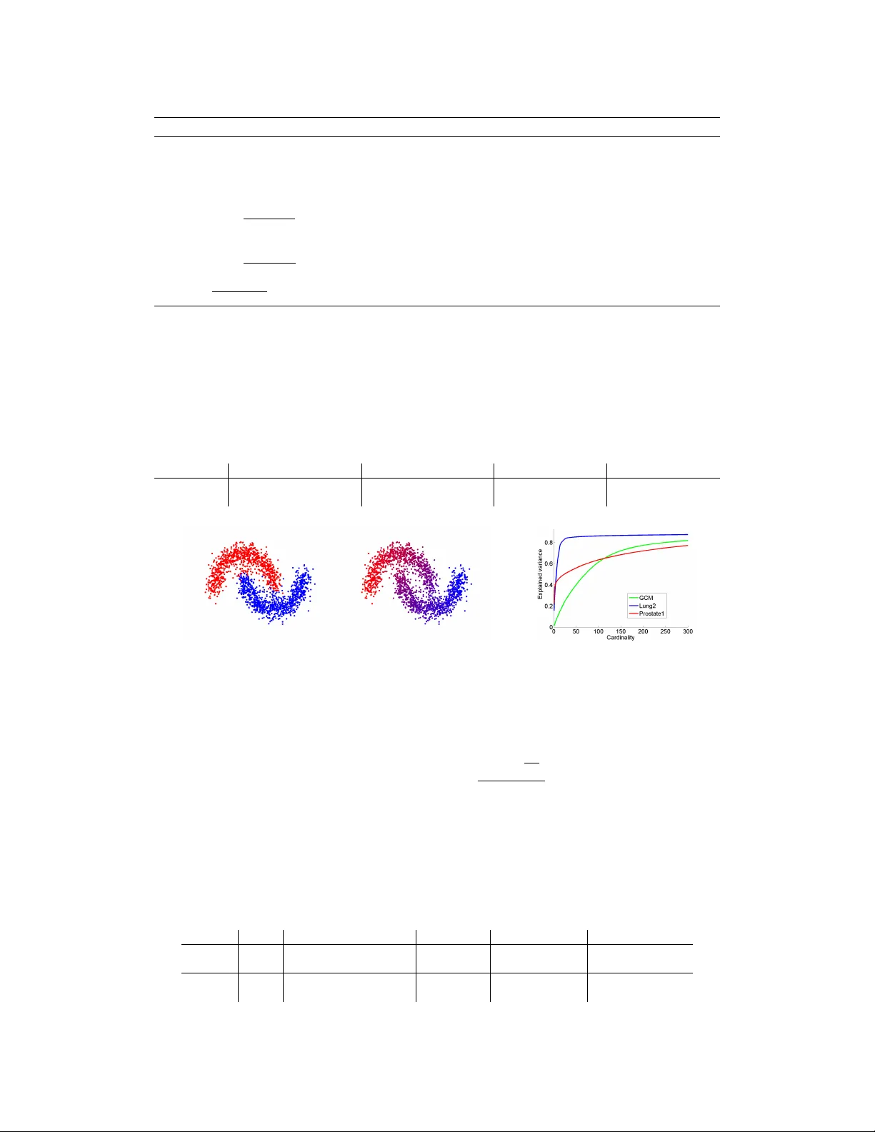
Many problems in machine learning and statistics can be formulated as (generalized) eigenproblems. In terms of the associated optimization problem, computing linear eigenvectors amounts to finding critical points of a quadratic function subject to qu…
Authors: Matthias Hein, Thomas B"uhler
An In verse P ower Method f or Nonlinear Eigenpr oblems with A pplications in 1 -Spectral Clustering and Sparse PCA Matthias Hein Thomas B ¨ uhler Saarland Univ ersity , Saarbr ¨ ucken, Germany { hein,tb } @cs.uni-saarland.de Abstract Many problems in machine learning and statistics can be formulated as (general- ized) eigenproblems. In terms of the associated optimization problem, comput- ing linear eigen vectors amounts to finding critical points of a quadratic function subject to quadratic constraints. In this paper we show that a certain class of con- strained optimization problems with nonquadratic objecti ve and constraints can be understood as nonlinear eigenpr oblems . W e deri ve a generalization of the in verse power method which is guaranteed to con ver ge to a nonlinear eigen vector . W e apply the in verse power method to 1-spectral clustering and sparse PCA which can naturally be formulated as nonlinear eigenproblems. In both applications we achiev e state-of-the-art results in terms of solution quality and runtime. Moving beyond the standard eigenproblem should be useful also in man y other applica- tions and our in verse po wer method can be easily adapted to new problems. 1 Introduction Eigen value problems associated to a symmetric and positiv e semi-definite matrix are quite abundant in machine learning and statistics. Howe ver , considering the eigenproblem from a v ariational point of view using Courant-Fischer-theory , the objectiv e is a ratio of quadratic functions, which is quite restrictiv e from a modeling perspectiv e. W e show in this paper that using a ratio of p -homogeneous functions leads quite naturally to a nonlinear eigen value problem, associated to a certain nonlin- ear operator . Clearly , such a generalization is only interesting if certain properties of the standard problem are preserved and efficient algorithms for the computation of nonlinear eigenv ectors are av ailable. In this paper we present an ef ficient generalization of the inv erse power method (IPM) to nonlinear eigen value problems and study the relation to the standard problem. While our IPM is a general purpose method, we show for two unsupervised learning problems that it can be easily adapted to a particular application. The first application is spectral clustering [22]. In prior work [6] we proposed p -spectral clustering based on the graph p -Laplacian, a nonlinear operator on graphs which reduces to the standard graph Laplacian for p = 2 . For p close to one, we obtained much better cuts than standard spectral clus- tering, at the cost of higher runtime. Using the ne w IPM, we ef ficiently compute eigen vectors of the 1 -Laplacian for 1 -spectral clustering. Similar to the recent work of [21], we improv e considerably compared to [6] both in terms of runtime and the achieved Cheeger cuts. Howe ver , opposed to the suggested method in [21] our IPM is guaranteed to con ver ge to an eigen vector of the 1 -Laplacian. The second application is sparse Principal Component Analysis (PCA). The moti vation for sparse PCA is that the largest PCA component is difficult to interpret as usually all components are nonzero. In order to allow a direct interpretation it is therefore desirable to have only a fe w features with nonzero components but which still e xplain most of the v ariance. This kind of trade-of f has been 1 widely studied in recent years, see [16] and references therein. W e sho w that also sparse PCA has a natural formulation as a nonlinear eigen value problem and can be ef ficiently solved with the IPM. 2 Nonlinear Eigenproblems The standard eigenproblem for a symmetric matric A ∈ R n × n is of the form Af − λf = 0 , (1) where f ∈ R n and λ ∈ R . It is a well-kno wn result from linear algebra that for symmetric matrices A , the eigen vectors of A can be characterized as critical points of the functional F Standard ( f ) = h f , Af i k f k 2 2 . (2) The eigenv ectors of A can be computed using the Courant-Fischer Min-Max principle. While the ratio of quadratic functions is useful in sev eral applications, it is a severe modeling restriction. This restriction howev er can be overcome using nonlinear eigenproblems. In this paper we consider functionals F of the form F ( f ) = R ( f ) S ( f ) , (3) where with R + = { x ∈ R | x ≥ 0 } we assume R : R n → R + , S : R n → R + to be con ve x, Lipschitz continuous, e ven and positi vely p -homogeneous 1 with p ≥ 1 . Moreov er, we assume that S ( f ) = 0 if and only if f = 0 . The condition that R and S are p -homogeneous and ev en will imply for any eigen vector v that also αv for α ∈ R is an eigen vector . It is easy to see that the functional of the standard eigen value problem in Equation (2) is a special case of the general functional in (3). T o gain some intuition, let us first consider the case where R and S are dif ferentiable. Then it holds for ev ery critical point f ∗ of F , ∇ F ( f ∗ ) = 0 ⇐ ⇒ ∇ R ( f ∗ ) − R ( f ∗ ) S ( f ∗ ) · ∇ S ( f ∗ ) = 0 . Let r, s : R n → R n be the operators defined as r ( f ) = ∇ R ( f ) , s ( f ) = ∇ S ( f ) and λ ∗ = R ( f ∗ ) S ( f ∗ ) , we see that ev ery critical point f ∗ of F satisfies the nonlinear eigenpr oblem r ( f ∗ ) − λ ∗ s ( f ∗ ) = 0 , (4) which is in general a system of nonlinear equations, as r and s are nonlinear operators. If R and S are both quadratic, r and s are linear operators and one gets back the standard eigenproblem (1). Before we proceed to the general nondif ferentiable case, we hav e to introduce some important con- cepts from nonsmooth analysis. Note that F is in general nonconv ex and nondif ferentiable. In the following we denote by ∂ F ( f ) the g eneralized gradient of F at f according to Clarke [10], ∂ F ( f ) = { ξ ∈ R n F 0 ( f , v ) ≥ h ξ , v i , for all v ∈ R n } , where F 0 ( f , v ) = lim g → f , t → 0 sup F ( g + tv ) − F ( g ) t . In the case where F is conv ex, ∂ F is the subdif- ferential of F and F 0 ( f , v ) the directional deri vati ve for each v ∈ R n . A characterization of critical points of nonsmooth functionals is as follows. Definition 2.1 ([8]) A point f ∈ R n is a critical point of F , if 0 ∈ ∂ F . This generalizes the well-known fact that the gradient of a differentiable function vanishes at a critical point. W e now show that the nonlinear eigenproblem (4) is a necessary condition for a critical point and in some cases ev en sufficient. A useful tool is the generalized Euler identity . Theorem 2.1 ([23]) Let R : R n → R be a positively p -homog eneous and con vex continuous func- tion. Then, for eac h x ∈ R n and r ∗ ∈ ∂ R ( x ) it holds that h x, r ∗ i = p R ( x ) . 1 A function G : R n → R is positiv ely homogeneous of degree p if G ( γ x ) = γ p G ( x ) for all γ ≥ 0 . 2 The ne xt theorem characterizes the relation between nonlinear eigen vectors and critical points of F . Theorem 2.2 Suppose that R, S fulfill the stated conditions. Then a necessary condition for f ∗ being a critical point of F is 0 ∈ ∂ R ( f ∗ ) − λ ∗ ∂ S ( f ∗ ) , wher e λ ∗ = R ( f ∗ ) S ( f ∗ ) . (5) If S is continuously differ entiable at f ∗ , then this is also sufficient. Proof: Let f ∗ fulfill the general nonlinear eigenproblem in (5), where r ∗ ∈ ∂ R ( f ∗ ) , s ∗ ∈ ∂ S ( f ∗ ) , such that r ∗ − λ ∗ s ∗ = 0 . Then by Theorem 2.1, 0 = h f ∗ , r ∗ i − λ ∗ h f ∗ , s ∗ i = p R ( f ∗ ) − p λ ∗ S ( f ∗ ) , and thus λ ∗ = R ( f ∗ ) /S ( f ∗ ) . As R, S are Lipschitz continuous, we ha ve, see Prop. 2.3.14 in [10], ∂ R S ( f ) ⊆ S ( f ) ∂ R ( f ) − R ( f ) ∂ S ( f ) S ( f ) 2 . (6) Thus if f ∗ is a critical point, that is 0 ∈ ∂ F ( f ∗ ) , then 0 ∈ ∂ R ( f ∗ ) − R ( f ∗ ) S ( f ∗ ) ∂ S ( f ∗ ) given that f ∗ 6 = 0 . Moreo ver , by Prop. 2.3.14 in [10] we hav e equality in (6), if S is continuously differentiable at f ∗ and thus (5) implies that f ∗ is a critical point of F . Finally , the definition of the associated nonlinear operators in the nonsmooth case is a bit tricky as r and s can be set-valued. Howe ver , as we assume R and S to be Lipschitz, the set where R and S are nondifferentiable has measure zero and thus r and s are single-valued almost e verywhere. 3 The in verse power method f or nonlinear Eigenproblems A standard technique to obtain the smallest eigen value of a positi ve semi-definite symmetric matrix A is the in verse power method [13]. Its main building block is the f act that the iterative scheme Af k +1 = f k (7) con ver ges to the smallest eigen vector of A . T ransforming (7) into the optimization problem f k +1 = arg min u 1 2 h u, A u i − u, f k (8) is the motiv ation for the general IPM. The direct generalization tries to solve 0 ∈ r ( f k +1 ) − s ( f k ) or equiv alently f k +1 = arg min u R ( u ) − u, s ( f k ) , (9) where r ( f ) ∈ ∂ R ( f ) and s ( f ) ∈ ∂ S ( f ) . For p > 1 this leads directly to Algorithm 2, ho wev er for p = 1 the direct generalization fails. In particular , the ball constraint has to be introduced in Algorithm 1 as the objectiv e in the optimization problem (9) is otherwise unbounded from below . (Note that the 2-norm is only chosen for algorithmic con venience). Moreover , the introduction of λ k in Algorithm 1 is necessary to guarantee descent whereas in Algorithm 2 it w ould just yield a rescaled solution of the problem in the inner loop (called inner problem in the following). For both methods we show con vergence to a solution of (4), which by Theorem 2.2 is a neces- sary condition for a critical point of F and often also sufficient. Interestingly , both applications are naturally formulated as 1 -homogeneous problems so that we use in both cases Algorithm 1. Ne ver- theless, we state the second algorithm for completeness. Note that we cannot guarantee con ver gence to the smallest eigenv ector even though our experiments suggest that we often do so. Howe ver , as the method is fast one can af ford to run it multiple times with different initializations and use the eigen vector with smallest eigen value. The inner optimization problem is con vex for both algorithms. In turns out that both for 1 -spectral clustering and sparse PCA the inner problem can be solved very ef ficiently , for sparse PCA it has 3 Algorithm 1 Computing a nonlinear eigen vector for con vex positi vely p -homogeneous functions R and S with p = 1 1: Initialization: f 0 = random with f 0 = 1 , λ 0 = F ( f 0 ) 2: repeat 3: f k +1 = arg min k u k 2 ≤ 1 R ( u ) − λ k u, s ( f k ) where s ( f k ) ∈ ∂ S ( f k ) 4: λ k +1 = R ( f k +1 ) /S ( f k +1 ) 5: until | λ k +1 − λ k | λ k < 6: Output: eigen value λ k +1 and eigen vector f k +1 . Algorithm 2 Computing a nonlinear eigen vector for con vex positi vely p -homogeneous functions R and S with p > 1 1: Initialization: f 0 = random, λ 0 = F ( f 0 ) 2: repeat 3: g k +1 = arg min u R ( u ) − u, s ( f k ) where s ( f k ) ∈ ∂ S ( f k ) 4: f k +1 = g k +1 /S ( g k +1 ) 1 /p 5: λ k +1 = R ( f k +1 ) /S ( f k +1 ) 6: until | λ k +1 − λ k | λ k < 7: Output: eigen value λ k +1 and eigen vector f k +1 . ev en a closed form solution. While we do not yet have results about conv ergence speed, empirical observation sho ws that one usually conv erges quite quickly to an eigen vector . T o our best kno wledge both suggested methods have not been considered before. In [5] they propose an in verse po wer method specially tailored to wards the continuous p -Laplacian for p > 1 , which can be seen as a special case of Algorithm 2. In [16] a generalized power method has been proposed which will be discussed in Section 5. Finally , both methods can be easily adapted to compute the largest nonlinear eigen value, which ho wev er we hav e to omit due to space constraints. Lemma 3.1 The sequences f k pr oduced by Alg. 1 and 2 satisfy F ( f k ) > F ( f k +1 ) for all k ≥ 0 or the sequences terminate. Theorem 3.1 The sequences f k pr oduced by Algorithms 1 and 2 conver ge to an eigen vector f ∗ with eigen value λ ∗ ∈ 0 , F ( f 0 ) in the sense that it solves the nonlinear eigenpr oblem (5) . If S is continuously differ entiable at f ∗ , then F has a critical point at f ∗ . Throughout the proofs, we use the notation Φ f k ( u ) = R ( u ) − λ k u, s ( f k ) and Ψ f k ( u ) = R ( u ) − u, s ( f k ) for the objectiv es of the inner problems in Algorithms 1 & 2, respectiv ely . Proof of Lemma 3.1 f or Algorithm 1: First note that the optimal v alue of the inner problem is non-positiv e as Φ f k (0) = 0 . Moreover , as Φ f k is 1 -homogeneous, the minimum of Φ f k is always attained at the boundary of the constraint set. Thus any f k fulfills f k 2 2 = 1 and thus is feasible, and min k f k 2 2 ≤ 1 Φ f k ( f ) ≤ Φ f k ( f k ) = R ( f k ) − λ k f k , s ( f k ) = R ( f k ) − F ( f k ) · S ( f k ) = 0 , where we used f k , s ( f k ) = S ( f k ) from Theorem 2.1. If the optimal value is zero, then f k is a possible minimizer and the sequence terminates and f k is an eigen vector see proof of Theorem 3.1 for Algorithm 1. Otherwise the optimal value is negati ve and at the optimal point f k +1 we get R ( f k +1 ) < λ k f k +1 , s ( f k ) . The definition of the subdifferential s ( f k ) together with the 1 - homogeneity of S yields S ( f k +1 ) ≥ S ( f k ) + f k +1 − f k , s ( f k ) = f k +1 , s ( f k ) , and finally F ( f k +1 ) = R ( f k +1 ) S ( f k +1 ) < λ k = F ( f k ) . 4 Proof of Theorem 3.1 for Algorithm 1: By Lemma 3.1 the sequence F ( f k ) is monotonically decreasing. By assumption S and R are nonnegati ve and hence F is bounded below by zero. Thus we hav e con vergence to wards a limit λ ∗ = lim k →∞ F ( f k ) . Note that f k 2 2 ≤ 1 for e very k , thus the sequence f k is contained in a compact set, which implies that there exists a subsequence f k j con ver ging to some element f ∗ . As the sequence F ( f k j ) is a subsequence of a con ver gent sequence, it has to con verge to wards the same limit, hence also lim j →∞ F ( f k j ) = λ ∗ . As shown before, the objecti ve of the inner optimization problem is nonpositi ve at the optimal point. Assume now that min k f k 2 2 ≤ 1 Φ f ∗ ( f ) < 0 . Then the vector f ∗∗ = arg min k f k 2 2 ≤ 1 Φ f ∗ ( f ) satisfies R ( f ∗∗ ) < λ ∗ h f ∗∗ , s ( f ∗ ) i = λ ∗ ( S ( f ∗ ) + h f ∗∗ − f ∗ , s ( f ∗ ) i ) ≤ λ ∗ S ( f ∗∗ ) , where we used the definition of the subdifferential and the 1 -homogeneity of S . Hence F ( f ∗∗ ) < λ ∗ = F ( f ∗ ) , which is a contradiction to the f act that the sequence F ( f k ) has con verged to λ ∗ . Thus we must hav e min k f k 2 2 ≤ 1 Φ f ∗ ( f ) = 0 , i.e. the function Φ f ∗ ( f ) is nonne gativ e in the unit ball. Using the fact that for any α ≥ 0 , Φ f ∗ ( αf ) = α Φ f ∗ , we can ev en conclude that the function Φ f ∗ ( f ) is nonnegati ve everywhere, and thus min f Φ f ∗ ( f ) = 0 . Note that Φ f ∗ ( f ∗ ) = 0 , which implies that f ∗ is a global minimizer of Φ f ∗ , and hence 0 ∈ ∂ Φ f ∗ ( f ∗ ) = ∂ R ( f ∗ ) − λ ∗ ∂ S ( f ∗ ) , which implies that f ∗ is an eigen vector with eigen value λ ∗ . Note that this argument was independent of the choice of the subsequence, thus every con vergent subsequence con ver ges to an eigenv ector with the same eigen value λ ∗ . Clearly we ha ve λ ∗ ≤ F ( f 0 ) . The following lemma is useful in the con ver gence proof of Algorithm 2. Lemma 3.2 Let R be a conve x, positively p -homogeneous function with p ≥ 1 . Then for any x ∈ R n , t ≥ 0 and any r ∗ ∈ ∂ R ( x ) we have t p − 1 r ∗ ∈ ∂ R ( tx ) . Proof: Using the definition of the subgradient, we have for an y y ∈ R n and any t ≥ 0 , t p R ( y ) ≥ t p R ( x ) + t p h r ∗ , y − x i . Using the p -homogeneity of R , we can rewrite this as R ( ty ) ≥ R ( tx ) + t p − 1 r ∗ , ty − tx , which implies t p − 1 r ∗ ∈ ∂ R ( tx ) . The following Proposition generalizes a result by Zarantonello [24]. Proposition 3.1 Let R : R n → R be a con vex, continuous and positively p -homogeneous and even functional and ∂ R ( f ) its subdif fer ential at f . Then it holds for any f , g ∈ R n and r ( f ) ∈ ∂ R ( f ) , |h r ( f ) , g i| ≤ h r ( f ) , f i 1 − 1 p h r ( g ) , g i 1 p = p · R ( f ) 1 − 1 p R ( g ) 1 p . Proof: First observe that for any k points x 0 , . . . x k − 1 ∈ R n , the subdifferential inequality yields R ( x l ) ≥ R ( x l − 1 ) + h r ( x l − 1 ) , x l − x l − 1 i , ∀ 1 ≤ l ≤ k − 1 R ( x 0 ) ≥ R ( x k − 1 ) + h r ( x k − 1 ) , x 0 − x k − 1 i , 5 and hence, by summing up, h r ( x 0 ) , x 1 − x 0 i + · · · + h r ( x k − 2 ) , x k − 1 − x k − 2 i + h r ( x k − 1 ) , x 0 − x k − 1 i ≤ 0 . (10) Let no w f , g ∈ R n , and r ( f ) ∈ ∂ R ( f ) , r ( g ) ∈ ∂ R ( g ) . W e construct a set of 2 m points x 0 , . . . x 2 m − 1 in R n , where m ∈ N , as follo ws: x i = i +1 m f , 0 ≤ i ≤ m − 1 2 m − 1 − i m g , m ≤ i ≤ 2 m − 1 . By Lemma 3.2 for all i ∈ { 0 , . . . 2 m − 1 } there e xists an r ∗ ( x i ) ∈ ∂ R ( x i ) s.t. r ∗ ( x i ) = ( i +1 m p − 1 r ( f ) , 0 ≤ i ≤ m − 1 2 m − 1 − i m p − 1 r ( g ) , m ≤ i ≤ 2 m − 1 . Eq. (10) no w yields m − 2 X i =0 * i + 1 m p − 1 r ( f ) , 1 m f + + r ( f ) , m − 1 m g − f − 2 m − 2 X i = m * 2 m − 1 − i m p − 1 r ( g ) , 1 m g + + 0 · r ( g ) , 1 m f − 0 · g ≤ 0 which simplifies to 1 m m − 1 X j =1 j m p − 1 − 1 h r ( f ) , f i − 1 m m − 1 X j =1 j m p − 1 h r ( g ) , g i + m − 1 m h r ( f ) , g i ≤ 0 . (11) By letting m → ∞ we obtain for the two sums lim m →∞ 1 m m − 1 X j =1 j m p − 1 = lim m →∞ 1 m m − 1 m X j = 1 m , 2 m ,... j p − 1 = Z 1 0 j p − 1 d j = 1 p . Hence in total in the limit m → ∞ Eq. (11) becomes h r ( f ) , g i − 1 − 1 p h r ( f ) , f i − 1 p h r ( g ) , g i ≤ 0 . As the above inequality holds for all f , g ∈ R n , clearly we can no w perform the substitution f → t − 1 f , g → t p − 1 g , r ( f ) → t − ( p − 1) r ( f ) , r ( g ) → t ( p − 1) 2 r ( g ) , where t ∈ R + , which giv es h r ( f ) , g i − 1 − 1 p t − p h r ( f ) , f i − 1 p t p ( p − 1) h r ( g ) , g i ≤ 0 . (12) A local optimum with respect to t of the left side satisfies the necessary condition 0 = ( p − 1) t − p − 1 h r ( f ) , f i − ( p − 1) t p 2 − p − 1 h r ( g ) , g i = t − p − 1 ( p − 1) h r ( f ) , f i − t p 2 h r ( g ) , g i , which implies that t p = h r ( f ) , f i h r ( g ) , g i 1 p . Plugging this into (12) yields 0 ≥ h r ( f ) , g i − 1 − 1 p h r ( g ) , g i 1 p h r ( f ) , f i 1 − 1 p − 1 p h r ( f ) , f i 1 − 1 p h r ( g ) , g i 1 p = h r ( f ) , g i − h r ( f ) , f i 1 − 1 p h r ( g ) , g i 1 p . 6 By the homogeneity of R we then have h r ( f ) , g i ≤ h r ( f ) , f i 1 − 1 p h r ( g ) , g i 1 p = p · R ( f ) 1 − 1 p R ( g ) 1 p . Finally , note that we can replace the left side by its absolute value since replacing g with − g yields h r ( f ) , − g i ≤ p · R ( f ) 1 − 1 p R ( − g ) 1 p = p · R ( f ) 1 − 1 p R ( g ) 1 p , where we used the fact that R is ev en. Proof of Lemma 3.1 f or Algorithm 2: Note that as R ( u ) ≥ 0 , the minimum of the objectiv e of the inner problem is attained for some u with u, s ( f k ) > 0 . Choose u such that u, s ( f k ) > 0 . Then we minimize Ψ f k on the ray tu , t ≥ 0 . W e hav e Ψ f k ( tu ) = R ( tu ) − t u, s ( f k ) = t p R ( u ) − t u, s ( f k ) and hence ∂ ∂ t Ψ f k ( tu ) = p t p − 1 R ( u ) − u, s ( f k ) and thus the minimum is attained at t ∗ ( u ) = h u,s ( f k ) i p R ( u ) 1 p − 1 > 0 and Ψ f k ( t ∗ ( u ) u ) = t ∗ ( u ) p R ( u ) − t ∗ ( u ) u, s ( f k ) = (1 − p ) u, s ( f k ) p p p R ( u ) 1 p − 1 . Assume there exists u that satisfies Ψ f k ( u ) < Ψ f k ( ˆ f ) where ˆ f = F ( f k ) 1 1 − p f k . Hence, also Ψ f k ( t ∗ ( u ) u ) < Ψ f k ( ˆ f ) , which implies (1 − p ) u, s ( f k ) p p p R ( u ) 1 p − 1 < F ( f k ) p 1 − p R ( f k ) − F ( f k ) 1 1 − p f k , s ( f k ) = F ( f k ) 1 1 − p (1 − p ) , where we used the fact that f k , s ( f k ) = pS ( f k ) and S ( f k ) = 1 . Rearranging, we obtain F ( f k ) > p p R ( u ) h u, s ( f k ) i p . Using the H ¨ older-type inequality of Proposition 3.1 and S ( f k ) = 1 , we obtain u, s ( f k ) ≤ pS ( f k ) 1 − 1 p S ( u ) 1 p = pS ( u ) 1 p , which gives F ( f k ) > F ( u ) . Let no w f ∗ be the minimizer of Ψ f k . Then f ∗ satisfies Ψ f k ( f ∗ ) ≤ Ψ f k ( ˆ f ) . If equality holds then ˆ f = F ( f k ) 1 1 − p f k is a minimizer of the inner problem and the sequence terminates. In this case f k is an eigen vector , see proof of Theorem 3.1 for Algorithm 2. Otherwise Ψ f k ( f ∗ ) < Ψ f k ( ˆ f ) and thus u = f ∗ fulfills the above assumption and we get F ( f k ) > F ( f ∗ ) , as claimed. Proof of Theorem 3.1 f or Algorithm 2: Note that as F ( f ) ≥ 0 , the sequence F ( f k ) is bounded from below , and by Lemma 3.1 it is monotonically decreasing and thus conv erges to some λ ∗ ∈ [0 , F ( f 0 )] . Moreo ver , S ( f k ) = 1 for all k . As S is continuous it attains its minimum m on the unit sphere in R n . By assumption m > 0 . W e obtain 1 = S ( f k ) = S f k k f k k 2 f k 2 ≥ m f k p 2 , = ⇒ f k 2 ≤ 1 m 1 p . Thus the sequence f k is bounded and there exists a conv ergent subsequence f k j . Clearly , lim j →∞ F ( f k j ) = lim k →∞ F ( f k ) = λ ∗ . Let now f ∗ = lim j →∞ f k j , and suppose that there exists u ∈ R n with Ψ f ∗ ( u ) < Ψ f ∗ ( ˆ f ) where ˆ f = F ( f ∗ ) 1 1 − p f ∗ . Then, analogously to the proof of 7 Lemma 3.1, one can conclude that F ( u ) < F ( f ∗ ) = λ ∗ which contradicts the fact that F ( f k j ) has as its limit λ ∗ . Thus ˆ f is a minimizer of Ψ f ∗ , which implies 0 ∈ ∂ Ψ f ∗ F ( f ∗ ) 1 1 − p f ∗ = ∂ R F ( f ∗ ) 1 1 − p f ∗ − s ( f ∗ ) = F ( f ∗ ) 1 1 − p p − 1 ∂ R ( f ∗ ) − s ( f ∗ ) = 1 F ( f ∗ ) ∂ R ( f ∗ ) − F ( f ∗ ) s ( f ∗ ) , so that f ∗ is an eigen vector with eigen value λ ∗ . As this argument was independent of the subse- quence, any con vergent subsequence of f k con ver ges tow ards an eigen vector with eigen value λ ∗ . Practical implementation: By the proof of Lemma 3.1, descent in F is not only guaranteed for the optimal solution of the inner problem, but for any vector u which has inner objective value Φ f k ( u ) < 0 = Φ f k ( f k ) for Alg. 1 and Ψ f k ( u ) < Ψ f k ( F ( f k ) 1 1 − p f k ) in the case of Alg. 2. This has two important practical implications. First, for the con vergence of the IPM, it is suf ficient to use a vector u satisfying the above conditions instead of the optimal solution of the inner problem. In particular , in an early stage where one is far away from the limit, it makes no sense to in vest much effort to solv e the inner problem accurately . Second, if the inner problem is solved by a descent method, a good initialization for the inner problem at step k + 1 is gi ven by f k in the case of Alg. 1 and F ( f k ) 1 1 − p f k in the case of Alg. 2 as descent in F is guaranteed after one step. 4 A pplication 1: 1 -spectral clustering and Cheeger cuts Spectral clustering is a graph-based clustering method (see [22] for an overvie w) based on a re- laxation of the NP-hard problem of finding the optimal balanced cut of an undirected graph. The spectral relaxation has as its solution the second eigen vector of the graph Laplacian and the final par- tition is found by optimal thresholding. While usually spectral clustering is understood as relaxation of the so called ratio/normalized cut, it can be equally seen as relaxation of the ratio/normalized Cheeger cut, see [6]. Giv en a weighted undirected graph with vertex set V and weight matrix W , the ratio Cheeger cut ( R CC ) of a partition ( C, C ) , where C ⊂ V and C = V \ C , is defined as R CC( C , C ) := cut( C, C ) min {| C | , C } , where cut( A, B ) = X i ∈ A,j ∈ B w ij , where we assume in the following that the graph is connected. Due to limited space the normalized version is omitted, but the proposed IPM can be adapted to this case. In [6] we proposed p -spectral clustering, a generalization of spectral clustering based on the second eigen vector of the nonlinear graph p -Laplacian (see [2]; the graph Laplacian is recov ered for p = 2 ). The main motiv ation was the relation between the optimal Cheeger cut h RCC = min C ⊂ V R CC( C , C ) and the Chee ger cut h ∗ RCC obtained by optimal thresholding the second eigen vector of the p -Laplacian, see [6, 9], ∀ p > 1 , h RCC max i ∈ V d i ≤ h ∗ RCC max i ∈ V d i ≤ p h RCC max i ∈ V d i 1 p , where d i = P i ∈ V w ij denotes the de gree of verte x i . While the inequality is quite loose for spectral clustering ( p = 2 ), it becomes tight for p → 1 . Indeed in [6] much better cuts than standard spectral clustering were obtained, at the expense of higher runtime. In [21] the idea w as taken up and they considered directly the variational characterization of the ratio Chee ger cut, see also [2, 9], h RCC = min f nonconstant 1 2 P n i,j =1 w ij | f i − f j | k f − median( f ) 1 k 1 = min f nonconstant median(f )=0 1 2 P n i,j =1 w ij | f i − f j | k f k 1 . (13) In [21] they proposed a minimization scheme based on the Split Bregman method [12]. Their method produces comparable cuts to the ones in [6], while being computationally much more efficient. Howe ver , they could not provide an y con vergence guarantee about their method. In this paper we consider the functional associated to the 1 -Laplacian ∆ 1 , F 1 ( f ) = 1 2 P n i,j =1 w ij | f i − f j | k f k 1 = h f , ∆ 1 f i k f k 1 , (14) 8 where (∆ 1 f ) i = n n X j =1 w ij u ij | u ij = − u j i , u ij ∈ sign( f i − f j ) o and sign( x ) = ( − 1 , x < 0 , [ − 1 , 1] , x = 0 , 1 , x > 0 . and study its associated nonlinear eigenproblem 0 ∈ ∆ 1 f − λ sign( f ) . Proposition 4.1 Any non-constant eig en vector f ∗ of the 1 -Laplacian has median zer o. Mor eover , let λ 2 be the second eigen value of the 1 -Laplacian, then if G is connected it holds λ 2 = h RCC . Proof: The subdifferential of the enumerator of F 1 can be computed as ∂ 1 2 n X i,j =1 w ij | f i − f j | i = n n X j =1 w ij u ij | u ij = − u j i , u ij ∈ sign( f i − f j ) o , where we use the set-valued mapping sign( x ) = ( − 1 , x < 0 , [ − 1 , 1] , x = 0 , 1 , x > 0 . Moreov er , the subdifferential of the denominator of F 1 is ∂ k f k 1 = sign( f ) . Note that, assuming that the graph is connected, an y non-constant eigen vector f ∗ must have λ ∗ > 0 . Thus if f ∗ is an eigen vector of the 1 -Laplacian, there must e xist u ij with u ij = − u j i and u ij ∈ sign( f ∗ i − f ∗ j ) and α i with α i ∈ sign( f ∗ i ) such that 0 = n X j =1 w ij u ij − λ ∗ α i . Summing o ver i yields due to the anti-symmetry of u ij , P i α i = | f ∗ + | − | f ∗ − | + P f ∗ i =0 α i = 0 , where | f ∗ + | , | f ∗ − | are the cardinalities of the positi ve and negati ve part of f ∗ and | f ∗ 0 | is the number of components with value zero. Thus we get | f ∗ + | − | f ∗ − | ≤ | f ∗ 0 | , which implies with | f ∗ + | + | f ∗ − | + | f ∗ 0 | = | V | that | f ∗ + | ≤ | V | 2 and | f ∗ − | ≤ | V | 2 . Thus the median of f ∗ is zero if | V | is odd. If | V | is ev en, the median is non-unique and is contained in [max f ∗ − , min f ∗ + ] which contains zero. If the graph is connected, the only eigen vector corresponding to the first eigen value λ 1 = 0 of the 1 -Laplacian is the constant one. As all non-constant eigenv ectors have median zero, it follows with Equation 13 that λ 2 ≥ h RCC . For the other direction, we hav e to use the algorithm we present in the following and some subsequent results. By Lemma 4.2 there exists a vector f ∗ = 1 C with | C | ≤ C such that F 1 ( f ∗ ) = h RCC . Ob viously , f ∗ is non-constant and has median zero and thus can be used as initial point f 0 for Algorithm 3. By Lemma 4.1 starting with f 0 = f ∗ the sequence either terminates and the current iterate f 0 is an eigen vector or one finds a f 1 with F 1 ( f 1 ) < F 1 ( f 0 ) , where f 1 has median zero. Suppose that there e xists such a f 1 , then F 1 ( f 1 ) < F 1 ( f 0 ) = min f nonconstant median(f )=0 F 1 ( f ) which is a contradiction. Therefore the sequence has to terminate and thus by the ar gument in the proof of Theorem 4.1 the corresponding iterate is an eigen vector . Thus we get h RCC ≥ λ 2 and thus with λ 2 ≥ h RCC we arriv e at the desired result. For the computation of the second eigen vector we ha ve to modify the IPM which is discussed in the next section. 9 4.1 Modification of the IPM f or computing the second eigen vector of the 1 -Laplacian The direct minimization of (14) would be compatible with the IPM, b ut the global minimizer is the first eigen vector which is constant. For computing the second eigen vector note that, unlike in the case p = 2 , we cannot simply project on the space orthogonal to the constant eigenv ector , since mutual orthogonality of the eigen vectors does not hold in the nonlinear case. Algorithm 3 is a modification of Algorithm 1 which computes a nonconstant eigenv ector of the 1- Laplacian. The notation | f k +1 + | , | f k +1 − | and | f k +1 0 | refers to the cardinality of positive, ne gativ e and zero elements, respecti vely . Note that Algorithm 1 requires in each step the computation of some subgradient s ( f k ) ∈ ∂ S ( f k ) , whereas in Algorithm 3 the subgradient v k has to satisfy v k , 1 = 0 . This condition ensures that the inner objective is in variant under addition of a constant and thus not affected by the subtraction of the median. Opposite to [21] we can prove conv ergence to a nonconstant eigen vector of the 1 -Laplacian. Ho wever , we cannot guarantee conv ergence to the second eigen vector . Thus we recommend to use multiple random initializations and use the result which achiev es the best ratio Cheeger cut. Algorithm 3 Computing a nonconstant 1 -eigen vector of the graph 1 -Laplacian 1: Input: weight matrix W 2: Initialization: nonconstant f 0 with median( f 0 ) = 0 and f 0 1 = 1 , accuracy 3: repeat 4: g k +1 = arg min k f k 2 2 ≤ 1 n 1 2 P n i,j =1 w ij | f i − f j | − λ k f , v k o 5: f k +1 = g k +1 − median g k +1 6: v k +1 i = ( sign( f k +1 i ) , if f k +1 i 6 = 0 , − | f k +1 + |−| f k +1 − | | f k +1 0 | , if f k +1 i = 0 . , 7: λ k +1 = F 1 ( f k +1 ) 8: until | λ k +1 − λ k | λ k < Lemma 4.1 The sequence f k pr oduced by Algorithm 3 satisfies F 1 ( f k ) > F 1 ( f k +1 ) for all k ≥ 0 or the sequence terminates. Proof: Note that, analogously to the proof of Lemma 3.1, we can conclude that the inner objectiv e is nonpositive at the optimum, where the sequence terminates if the optimal value is zero as the previous f k is among the minimizers of the inner problem. Now observe that the objectiv e of the inner optimization problem is in variant under addition of a constant. This follows from the fact that we always ha ve v k , 1 = 0 , which can be easily verified. Hence, with R ( f ) = 1 2 P n i,j =1 w ij | f i − f j | , we get R ( f k +1 ) − λ k f k +1 , v k = R ( g k +1 ) − λ k g k +1 , v k < 0 . Dividing both sides by f k +1 1 yields R ( f k +1 ) k f k +1 k 1 − λ k f k +1 , v k k f k +1 k 1 < 0 , and with f k +1 , v k ≤ f k +1 1 v k ∞ = f k +1 1 , the result follows. Theorem 4.1 The sequence f k pr oduced by Algorithm 3 con ver ges to an eigen vector f ∗ of the 1 - Laplacian with eigen value λ ∗ ∈ h RCC , F 1 ( f 0 ) . Furthermor e, F 1 ( f k ) > F 1 ( f k +1 ) for all k ≥ 0 or the sequence terminates. Proof: Note that ev ery constant vector u 0 satisfies Φ f k ( u 0 ) = 0 as v k , 1 = 0 . The minimizer of Φ f k is either negati ve or the sequence terminates in which case the previous non-constant g k is 10 a minimizer . In any case g k +1 cannot be constant and in turn f k +1 is nonconstant and has median zero. Thus for all k , F 1 ( f k ) = 1 2 P n i,j =1 w ij | f k i − f k j | k f k k 1 = 1 2 P n i,j =1 w ij | f k i − f k j | k f k − median( f k ) 1 k 1 ≥ h RCC , where we use that the median of f k is zero. Thus F 1 ( f k ) is lo wer-bounded by h RCC . Note that h RCC ≤ λ 2 . W e can conclude no w analogously to Theorem 3.1 that the sequence F 1 ( f k ) conv erges to some limit λ ∗ = lim k →∞ F 1 ( f k ) ≥ h RCC . As in Theorem 3.1 the compactness of the set containing the sequence g k implies the existence of a con ver gent subsequence g k j , and using the f act that subtracting the median is continuous we hav e lim j →∞ f k j = g ∗ − median( g ∗ ) 1 =: f ∗ . The proof now proceeds analogously to Theorem 3.1. 4.2 Quality guarantee f or 1 -spectral clustering Even though we cannot guarantee that we obtain the optimal ratio Cheeger cut, we can guarantee that 1 -spectral clustering always leads to a ratio Cheeger cut at least as good as the one found by standard spectral clustering. Let ( C ∗ f , C ∗ f ) be the partition of V obtained by optimal thresholding of f , where C ∗ f = arg min t R CC( C t f , C t f ) , and for t ∈ R , C t f = { i ∈ V | f i > t } . Furthermore, 1 C denotes the vector which is 1 on C and 0 else. Lemma 4.2 Let C , C be a partitioning of the vertex set V , and assume that | C | ≤ C . Then for any vector f ∈ R n of the form f = α 1 C , wher e α ∈ R , it holds that F 1 ( f ) = R CC( C , C ) . Proof: As F 1 is scale in variant, we can without loss of generality assume that α = 1 . Then we ha ve F 1 ( f ) = 1 2 P n i,j =1 w ij | f i − f j | k f k 1 = 1 2 P i ∈ C,j / ∈ C w ij + 1 2 P i / ∈ C,j ∈ C w ij P i ∈ C 1 = cut( C, C ) | C | = cut( C, C min | C | , C = R CC( C , C ) . Lemma 4.3 Let f ∈ R n with median( f ) = 0 , and C = arg min {| C ∗ f | , | C ∗ f |} . Then the vector f ∗ = 1 C satisfies F 1 ( f ) ≥ F 1 ( f ∗ ) . Proof: Denote by f + : V → R the function f + i := max { 0 , f i } , and analogously , let f − := max { 0 , − f i } . Then we ha ve R ( f ) = 1 2 X i,j w ij | f i − f j | = 1 2 X i,j w ij f + i − f − i − f + j + f − j . (15) Note that we always have f + i − f − i − f + j + f − j = f + i − f + j + f − i − f − j , which can easily be verified by performing a case distinction o ver the signs of f i and f j . Eq. (15) can no w be written as R ( f ) = 1 2 X i,j w ij f + i − f + j + 1 2 X i,j w ij f − i − f − j = R ( f + ) + R ( f − ) . Using the fact that k f k 1 can be decomposed as k f + k 1 + k f − k 1 , we obtain R ( f ) k f k 1 = R ( f + ) + R ( f − ) k f + k 1 + k f − k 1 ≥ min R ( f + ) k f + k 1 , R ( f − ) k f − k 1 . (16) 11 The last inequality follows from the f act that we always ha ve for a, b, c, d > 0 , a + b c + d ≥ min a c , b d , which can be easily shown by contradiction. Let wlog min a c , b d = a c , and assume that a + b c + d < a c . This implies a c > b d , which is a contradiction to a c ≤ b d . Note that median( f ) = 0 , hence we hav e 0 ∈ arg min c X i ∈ V | f i − c | , which implies that 0 ∈ ∂ P i ∈ V | f i | and hence there exist coef ficients | α i | ≤ 1 such that 0 = X f i 6 =0 sign( f i ) + X f i =0 α i , which is equiv alent to |{ i, f i > 0 }| − |{ i, f i < 0 }| ≤ |{ i, f i = 0 }| . This inequality implies that |{ i, f i > 0 }| ≤ | V | 2 and |{ i, f i < 0 }| ≤ | V | 2 . W e no w rewrite R ( f + ) as follows: R ( f + ) = 1 2 X f + i >f + j w ij f + i − f + j = X f + i >f + j w ij Z f + i f + j 1 dt = Z ∞ 0 X f + i >t ≥ f + j w ij dt . Note that for t ≥ 0 , X f + i >t ≥ f + j w ij = cut( C t f , C t f ) = cut( C t f , C t f ) min n C t f , C t f o · C t f ≥ R CC( C ∗ f , C ∗ f ) · C t f , where in the second step we used that C t f ≤ |{ i, f i > 0 }| ≤ | V | 2 . Hence we have R ( f + ) ≥ Z ∞ 0 R CC( C ∗ f , C ∗ f ) · C t f dt = R CC( C ∗ f , C ∗ f ) Z ∞ 0 X f i >t 1 dt = R CC( C ∗ f , C ∗ f ) X f i > 0 Z f i 0 1 dt = R CC( C ∗ f , C ∗ f ) f + 1 . Hence it holds that F 1 ( f + ) ≥ RCC( C ∗ f , C ∗ f ) , and analogously one shows that F 1 ( f − ) ≥ R CC( C ∗ − f , C ∗ − f ) . Note that R CC( C ∗ f , C ∗ f ) = R CC( C ∗ − f , C ∗ − f ) = F 1 ( f ∗ ) , by Lemma 4.2. Combining this with Eq. (16) yields the result. Theorem 4.2 Let u denote the second eigen vector of the standard graph Laplacian, and f denote the result of Algorithm 3 after initializing with the vector 1 | C | 1 C , wher e C = arg min {| C ∗ u | , | C ∗ u |} . Then R CC( C ∗ u , C ∗ u ) ≥ R CC( C ∗ f , C ∗ f ) . Proof: Using Lemma 4.1 and 4.2 , we have the follo wing chain of inequalities: R CC( C ∗ u , C ∗ u ) 4 . 2 = F 1 1 | C | 1 C = F 1 ( 1 C ) 4 . 1 ≥ F 1 ( f ) . W ith C 1 := arg min {| C ∗ f | , | C ∗ f |} , we obtain by Lemma 4.3 and 4.2: F 1 ( f ) 4 . 3 ≥ F 1 ( 1 C 1 ) 4 . 2 = RCC( C ∗ f , C ∗ f ) . 12 4.3 Solution of the inner pr oblem The inner problem is con ve x, thus a solution can be computed by any standard method for solving con ve x nonsmooth programs, e.g. subgradient methods [4]. Howe ver , in this particular case we can exploit the structure of the problem and use the equi valent dual formulation of the inner problem. Lemma 4.4 Let E ⊂ V × V denote the set of edges and A : R E → R V be defined as ( Aα ) i = P j | ( i,j ) ∈ E w ij α ij . The inner pr oblem is equivalent to min { α ∈ R E | k α k ∞ ≤ 1 , α ij = − α j i } Ψ( α ) := Aα − F ( f k ) v k 2 2 . The Lipschitz constant of the gr adient of Ψ is upper bounded by 2 max r P n s =1 w 2 rs . Proof: First, we note that 1 2 n X i,j =1 w ij | u i − u j | = max { β ∈ R E | k β k ∞ ≤ 1 } 1 2 X ( i,j ) ∈ E w ij ( u i − u j ) β ij . Introducing the new v ariable α ij = 1 2 ( β ij − β j i ) , this can be rewritten as max { α ∈ R E | k α k ∞ ≤ 1 , α ij = − α j i } X ( i,j ) ∈ E w ij α ij u i = max { α ∈ R E | k α k ∞ ≤ 1 , α ij = − α j i } h u, Aα i , where we hav e introduced the notation ( Aα ) i = P j | ( i,j ) ∈ E w ij α ij . Both u and α are constrained to lie in non-empty compact, conv ex sets, and thus we can reformulate the inner objecti ve by the standard min-max-theorem (see e.g. Corollary 37.3.2. in [18]) as follows: min k u k 2 ≤ 1 max { α ∈ R E | k α k ∞ ≤ 1 , α ij = − α j i } h u, Aα i − F ( f k ) u, v k = max { α ∈ R E | k α k ∞ ≤ 1 , α ij = − α j i } min k u k 2 ≤ 1 u, Aα − F ( f k ) v k = max { α ∈ R E | k α k ∞ ≤ 1 , α ij = − α j i } − Aα − F ( f k ) v k 2 . In the last step we have used that the solution of the minimization of the linear function o ver the Euclidean unit ball is giv en by u ∗ = − Aα − F ( f k ) v k k Aα − F ( f k ) v k k 2 , if Aα − F ( f k ) v k 6 = 0 and otherwise u ∗ is an arbitrary element of the Euclidean unit ball. T rans- forming the maximization problem into a minimization problem finishes the proof of the first state- ment. Re garding the Lipschitz constant, a straightforward computation sho ws that ( ∇ Ψ( α )) rs = 2 w rs X j | ( r,j ) ∈ E w rj α rj − F ( f k ) v k r . Thus, k∇ Ψ( α ) − ∇ Ψ( β ) k 2 = 4 X ( r,s ) ∈ E w 2 rs X j | ( r,j ) ∈ E w rj ( α rj − β rj ) 2 ≤ 4 X ( r,s ) ∈ E w 2 rs X j | ( r,j ) ∈ E w 2 rj X i | ( r ,i ) ∈ E ( α ri − β ri ) 2 = 4 n X r =1 X s | ( r ,s ) ∈ E w 2 rs 2 X i | ( r ,i ) ∈ E ( α ri − β ri ) 2 ≤ 4 max r n X s =1 w 2 rs 2 X ( r,i ) ∈ E ( α ri − β ri ) 2 . 13 Algorithm 4 Solution of the dual inner problem with FIST A 1: Input: Lipschitz-constant L of ∇ Ψ , 2: Initialization: t 1 = 1 , α 1 ∈ R E , 3: repeat 4: β t +1 rs = α t rs − 1 L ∇ Ψ( α t ) rs = α t rs − 2 L w rs X j | ( r,j ) ∈ E w rj α t rj − F ( f k ) v k r 5: t k +1 = 1+ √ 1+4 t 2 k 2 , 6: α t +1 rs = β t +1 rs + t k − 1 t k +1 β t +1 rs − β t rs . 7: until stop if gap between original and dual problem is smaller than Compared to the primal problem, the objectiv e of the dual problem is smooth. Moreover , it can be efficiently solved using FIST A ([3]), a two-step subgradient method with guaranteed con ver gence rate O ( 1 k 2 ) where k is the number of steps. The only input of FIST A is an upper bound on the Lips- chitz constant of the gradient of the objecti ve. FIST A provides a good solution in a fe w steps which guarantees descent in functional (13) and thus makes the modified IPM very fast. The resulting Algorithm is shown in Alg. 4. 5 A pplication 2: Sparse PCA Principal Component Analysis (PCA) is a standard technique for dimensionality reduction and data analysis [14]. PCA finds the k -dimensional subspace of maximal v ariance in the data. For k = 1 , giv en a data matrix X ∈ R n × p where each column has mean 0 , in PCA one computes f ∗ = arg max f ∈ R p f , X T X f k f k 2 2 , (17) where the maximizer f ∗ is the lar gest eigen vector of the covariance matrix Σ = X T X ∈ R p × p . The interpretation of the PCA component f ∗ is difficult as usually all components are nonzero. In sparse PCA one wants to get a small number of features which still capture most of the variance. For instance, in the case of gene e xpression data one would like the principal components to consist only of a few significant genes, making it easy to interpret by a human. Thus one needs to enforce sparsity of the PCA component, which yields a trade-off between e xplained variance and sparsity . While standard PCA leads to an eigenproblem, adding a constraint on the cardinality , i.e. the num- ber of nonzero coefficients, makes the problem NP-hard. The first approaches performed simple thresholding of the principal components which was sho wn to be misleading [7]. Since then se veral methods ha ve been proposed, mainly based on penalizing the L 1 norm of the principal components, including SCoTLASS [15] and SPCA [25]. D’Aspremont et al.[11] focused on the L 0 -constrained formulation and proposed a greedy algorithm to compute a full set of good candidate solutions up to a specified target sparsity , and deriv ed suf ficient conditions for a vector to be globally optimal. Moghaddam et al. [17] used branch and bound to compute optimal solutions for small problem instances. Other approaches include D.C. [20] and EM-based methods [19]. Recently , Journee et al. [16] proposed two single unit (computation of one component only) and two block (simultaneous computation of multiple components) methods based on L 0 -penalization and L 1 -penalization. Problem (17) is equiv alent to f ∗ = arg min f ∈ R p k f k 2 2 h f , Σ f i = arg min f ∈ R p k f k 2 k X f k 2 . 14 In order to enforce sparsity we use instead of the L 2 -norm a con vex combination of an L 1 norm and L 2 norm in the enumerator , which yields the functional F ( f ) = (1 − α ) k f k 2 + α k f k 1 k X f k 2 , (18) with sparsity controlling parameter α ∈ [0 , 1] . Standard PCA is recovered for α = 0 , whereas α = 1 yields the sparsest non-trivial solution: the component with the maximal variance. One easily sees that the formulation (18) fits in our general framework, as both enumerator and denominator are 1 -homogeneous functions. The inner problem of the IPM becomes g k +1 = arg min k f k 2 ≤ 1 (1 − α ) k f k 2 + α k f k 1 − λ k f , µ k , where µ k = Σ f k p h f k , Σ f k i . (19) This problem has a closed form solution. In the follo wing we use the notation x + = max { 0 , x } . Lemma 5.1 The con vex optimization pr oblem (19) has the analytical solution g k +1 i = 1 s sign( µ k i ) λ k µ k i − α + , wher e s = r X n i =1 ( λ k | µ k i | − α ) 2 + . Proof: W e note that the objecti ve is positively 1-homogeneous and that the optimum is either zero by plugging in the previous iterate or negativ e in which case the optimum is attained at the boundary . Thus wlog we can assume that at the optimum k f k 2 = 1 . Thus the problem reduces to min k f k 2 ≤ 1 α k f k 1 − λ k f , µ k . First, we deriv e an equiv alent “dual” problem, noting α k f k 1 − λ k µ k , f = max k v k ∞ ≤ 1 f , αv − λ k µ k . Using the fact that the objectiv e is con vex in f and concave in v and the feasible set is compact, we obtain by the min-max equality: min k f k 2 ≤ 1 max k v k ∞ ≤ 1 f , αv − λ k µ k = max k v k ∞ ≤ 1 min k f k 2 ≤ 1 f , αv − λ k µ k = max k v k ∞ ≤ 1 − αv − λ k µ k 2 . The objecti ve of the dual problem is separable in v and the constraints of v as well. Thus each component can be optimized separately which giv es v i = sign( µ k i ) min 1 , λ k | µ k i | α . Using that f ∗ = ( − αv + λ k µ k ) / λ k µ k − αv 2 , we get the solution f i = sign( µ k i )( λ k | µ k i | − α ) + q P n i =1 ( λ k | µ k i | − α ) 2 + . As s is just a scaling factor , we can omit it and obtain the simple and efficient scheme to compute sparse principal components shown in Algorithm 5. While the deriv ation is quite different from [16], the resulting algorithms are very similar . The subtle difference is that in our formulation the thresholding parameter of the inner problem depends on the current eigen v alue estimate whereas it is fixed in [16]. Empirically , this leads to the fact that we need slightly less iterations to con verge. 6 Experiments 1-Spectral Clustering: W e compare our IPM with the total variation (TV) based algorithm by [21], p -spectral clustering with p = 1 . 1 [6] as well as standard spectral clustering with optimal 15 Algorithm 5 Sparse PCA 1: Input: data matrix X , sparsity controlling parameter α , accuracy 2: Initialization: f 0 = random with S ( f k ) = 1 , λ 0 = F ( f k ) 3: repeat 4: g k +1 i = sign( µ k i ) λ k µ k i − α + , 5: f k +1 = g k +1 k X g k +1 k 2 6: λ k +1 = (1 − α ) f k +1 2 + α f k +1 1 7: µ k +1 = Σ f k +1 k X f k +1 k 2 8: until | λ k +1 − λ k | λ k < thresholding the second eigenv ector of the graph Laplacian ( p = 2 ). The graph and the two-moons dataset is constructed as in [6]. The following table sho ws the average ratio Chee ger cut (RCC) and error (classification as in [6]) for 100 draws of a tw o-moons dataset with 2000 points. In the case of the IPM, we use the best result of 10 runs with random initializations and one run initialized with the second eigen vector of the unnormalized graph Laplacian. For [21] we initialize once with the second eigen vector of the normalized graph Laplacian as proposed in [21] and 10 times randomly . IPM and the TV -based method yield similar results, slightly better than 1 . 1 -spectral and clearly outperforming standard spectral clustering. In terms of runtime, IPM and [21] are on the same le vel. In verse Po wer Method Szlam & Bresson [21] 1 . 1 -spectral [6] Standard spectral A vg. R CC 0.0195 ( ± 0.0015) 0.0195 ( ± 0.0015) 0.0196 ( ± 0.0016) 0.0247 ( ± 0.0016) A vg. error 0.0462 ( ± 0.0161) 0.0491 ( ± 0.0181) 0.0578 ( ± 0.0285) 0.1685 ( ± 0.0200) Figure 1: Left and middle: Second eigen vector of the 1-Laplacian and 2-Laplacian, respectively . Right: Relative V ariance (relative to maximal possible v ariance) versus number of non-zero compo- nents for the three datasets Lung2, GCM and Prostate1. Next we perform unnormalized 1 -spectral clustering on the full USPS and MNIST -datasets ( 9298 resp. 70000 points). As clustering criterion we use the multicut version of R Cut , given as R Cut( C 1 , . . . , C K ) = K X i =1 cut( C i , C i ) | C i | . W e successi vely subdivide clusters until the desired number of clusters ( K = 10 ) is reached. In each substep the eigen vector obtained on the subgraph is thresholded such that the multi-cut criterion is minimized. This recursive partitioning scheme is used for all methods. As in the pre vious e xperi- ment, we perform one run initialized with the thresholded second eigenv ector of the unnormalized graph Laplacian in the case of the IPM and with the second eigen vector of the normalized graph Laplacian in the case of [21]. In both cases we add 100 runs with random initializations. The next table shows the obtained R Cut and errors. In verse Po wer Method S.&B. [21] 1 . 1 -spectral [6] Standard spectral MNIST Rcut 0.1507 0.1545 0.1529 0.2252 Error 0.1244 0.1318 0.1293 0.1883 USPS Rcut 0.6661 0.6663 0.6676 0.8180 Error 0.1349 0.1309 0.1308 0.1686 Again the three nonlinear eigenv ector methods clearly outperform standard spectral clustering. Note that our method requires additional ef fort (100 runs) but we get better results. For both datasets our 16 method achie ves the best R Cut . Howe ver , if one wants to do only a single run, by Theorem 4.2 for bi-partitions one achiev es a cut at least as good as the one of standard spectral clustering if one initializes with the thresholded 2nd eigen vector of the 2-Laplacian. Sparse PCA: W e ev aluate our IPM for sparse PCA on gene expression datasets obtained from [1]. W e compare with two recent algorithms: the L 1 based single-unit power algorithm of [16] as well as the EM-based algorithm in [19]. For all considered datasets, the three methods achie ve very similar performance in terms of the tradeoff between explained v ariance and sparsity of the solution, see Fig.1 (Right). In fact the results are so similar that for each dataset, the plots of all three methods coincide in one line. In [16] it also has been observed that the best state-of-the-art algorithms produce the same trade-off curv e if one uses the same initialization strategy . Acknowledgments: This work has been supported by the Excellence Cluster on Multimodal Com- puting and Interaction at Saarland Univ ersity . References [1] http://www.stat.ucla.edu/ ˜ wxl/research/microarray/DBC/index.htm . [2] S. Amghibech. Eigenv alues of the discrete p-Laplacian for graphs. Ars Combinatoria , 67:283–302, 2003. [3] A. Beck and M. T eboulle. Fast gradient-based algorithms for constrained total v ariation image denoising and deblurring problems. IEEE T ransactions on Image Pr ocessing , 18(11):2419–2434, 2009. [4] D.P . Bertsekas. Nonlinear Pr ogramming . Athena Scientific, 1999. [5] R.J. Biezuner , G. Ercole, and E.M. Martins. Computing the first eigenv alue of the p -Laplacian via the in verse po wer method. Journal of Functional Analysis , 257:243–270, 2009. [6] T . B ¨ uhler and M. Hein. Spectral Clustering based on the graph p -Laplacian. In Proceedings of the 26th International Confer ence on Machine Learning , pages 81–88. Omnipress, 2009. [7] J. Cadima and I.T . Jolliffe. Loading and correlations in the interpretation of principal components. Journal of Applied Statistics , 22:203–214, 1995. [8] K.-C. Chang. V ariational methods for non-differentiable functionals and their applications to partial differential equations. Journal of Mathematical Analysis and Applications , 80:102–129, 1981. [9] F .R.K. Chung. Spectral Gr aph Theory . AMS, 1997. [10] F .H. Clarke. Optimization and Nonsmooth Analysis . W iley New Y ork, 1983. [11] A. d’Aspremont, F . Bach, and L. El Ghaoui. Optimal solutions for sparse principal component analysis. Journal of Mac hine Learning Resear ch , 9:1269–1294, 2008. [12] T . Goldstein and S. Osher . The Split Bregman method for L1-Regularized Problems. SIAM J ournal on Imaging Sciences , 2(2):323–343, 2009. [13] G.H. Golub and C.F . V an Loan. Matrix Computations . Johns Hopkins Uni versity Press, 3rd edition, 1996. [14] I.T . Jolliffe. Principal Component Analysis . Springer, 2nd edition, 2002. [15] I.T . Jolliffe, N. Trendafilo v , and M. Uddin. A modified principal component technique based on the LASSO. J ournal of Computational and Graphical Statistics , 12:531–547, 2003. [16] M. Journ ´ ee, Y . Nesterov , P . Richt ´ arik, and R. Sepulchre. Generalized Power Method for Sparse Principal Component Analysis. J ournal of Machine Learning Resear ch , 11:517–553, 2010. [17] B. Moghaddam, Y . W eiss, and S. A vidan. Spectral bounds for sparse PCA: Exact and greedy algorithms. In Advances in Neural Information Pr ocessing Systems , pages 915–922. MIT Press, 2006. [18] R.T . Rockafellar . Con vex analysis . Princeton University Press, 1970. [19] C.D. Sigg and J.M. Buhmann. Expectation-maximization for sparse and non-negati ve PCA. In Pr oceed- ings of the 25th International Confer ence on Machine Learning , pages 960–967. A CM, 2008. [20] B.K. Sriperumbudur , D.A. T orres, and G.R.G. Lanckriet. Sparse eigen methods by D.C. programming. In Pr oceedings of the 24th International Confer ence on Machine Learning , pages 831–838. A CM, 2007. [21] A. Szlam and X. Bresson. T otal variation and Cheeger cuts. In Pr oceedings of the 27th International Confer ence on Machine Learning , pages 1039–1046. Omnipress, 2010. [22] U. von Luxb urg. A tutorial on spectral clustering. Statistics and Computing , 17:395–416, 2007. [23] F . Y ang and Z. W ei. Generalized Euler identity for subdifferentials of homogeneous functions and appli- cations. Mathematical Analysis and Applications , 337:516–523, 2008. 17 [24] E. Zarantonello. The meaning of the Cauchy-Schwartz-Buniako vsky inequality . Pr oceedings of the American Mathematical Society , 59(1), 1976. [25] H. Zou, T . Hastie, and R. T ibshirani. Sparse principal component analysis. J ournal of Computational and Graphical Statistics , 15:265–286, 2006. 18
Original Paper
Loading high-quality paper...
Comments & Academic Discussion
Loading comments...
Leave a Comment