A New Approach to Population Sizing for Memetic Algorithms: A Case Study for the Multidimensional Assignment Problem

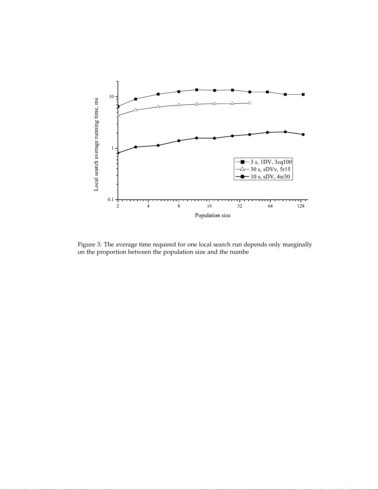
A New Approach to Populati on Sizing for Memetic Algorithms : A Case Study for the Multidimen sional Assignm ent Problem ∗ D. Karapetyan Daniel.Karapetyan@gmail.com Department of Computer Science, R oyal Holloway University of London, Egh am, Surrey , TW20 0EX, UK G. Gutin G.Gutin@cs.rhul .ac.uk Department of Computer S cience, Royal Holloway University of London, Egham, S ur- rey , TW20 0 E X, UK Abstract Memetic Algo rithms are known to be a power ful technique in solving hard optimi za- tion problems. T o design a memetic algor ithm one needs to make a host of decisions; selecting a population si ze is one of the most important among them. Most algor ithms in the literature ﬁx the population size to a certain constant value. This reduces the al- gorithm’s quality since the optimal population size varie s for different instances, lo cal search procedures and running times . In this paper we propose an adjustable popu- lation s ize. It is calculated as a function of the running time of the whole algori thm and the aver ag e running time of the l ocal se arch for the given instance. Note that in many applications the running time of a heuristic should be limited and therefore we use this limi t as a parameter of the algorithm. The average running time of the local search procedure is obtained dur ing the algor ithm’s run. Some coefﬁcients which are independent with respe ct to the instance or the l ocal search are to be tuned before the algorithm run; we provide a proced ure to ﬁnd these coefﬁcients. The proposed approach was used to develop a memetic algorithm for the Multidi - mensional Assignment Problem (MAP or s -AP in the case of s di mensions) which is an extension of the well-known assig nment problem. MAP is NP-hard and has a host of applications. W e s how that using adjustable population size m ak e s the algorithm ﬂexible to perform well for instances of very di fferent sizes and types and fo r different running times and local search es. This allows us to select the most efﬁcient local search for every instance type. The results o f computational experiments for several instance families and sizes prove that the proposed algo rithm performs efﬁciently for a wide range of the running times and clearly outperforms the s tate-of-the ar t 3-AP memetic algorithm being given the same time. Keywords Memetic Algorithm, Population Sizing, Parameter T uning, Parameter Control, Meta- heuristic, Multidimensional Assignment Problem. 1 Introduction A memetic algorithm is a combination of an e v olutionary algorithm with a local sea rch procedure (Krasnogor and Smith, 2005). The memetic approach is a te mplate for an ∗ A p reliminary version of th is paper was accepted for publication in proc eedings of t he Stochastic Local Search Conference 20 09 in Lecture Notes in Computer Science (Gutin and Karapetyan, 2009b). c  200X by the Massachusetts Institute of T echnology Evolutionary Computation x(x): xxx-xxx G. Gutin, D. Karapetyan algorithm rather than a set of rules f or de signing a powerful heuristic. A typical frame of a memetic algorithm is presented in Figure 1 (for a formal deﬁnition of a memetic algorithm main loop see, e .g., Krasnogor and Smith (2008)). 1. Produce the ﬁrst generation, i.e., a set of feasible solutions. 2. A pply a local search procedure to every solution in the ﬁrst generation. 3. Repe a t the following while a termination criterion is not met: (a) Produce a set of new solutions by applying so-called genetic opera tors to so- lutions from the previous gener a tion. (b) Improve e very solution in this set with the local search procedure. (c) Select severa l best solutions f rom this set to the next generation. Figure 1: A typical memetic algorithm frame. When implementing a memetic algorithm, one fa ces a lot of questions. Some of these questions, like selecting the most appropriate local search or crossover operators, were widely discussed in the literature while others are still not investigated enough. In this research we focus our attention on the population sizing. Population size is the number of soluti ons (chromosom es) maintained at a time by a memetic algorithm. M a ny researchers indicate the importance of selecting proper population sizes (Glover a nd Kochenberger, 2 0 03; Ha rik et al., 19 99; Har t et al., 2005). However , the most usual way to deﬁne the population size is to ﬁx it to some constant at the design time ( Cotta, 2008; Grefenstette, 1986; Hart et al., 20 0 5; Huang and L im, 2006). Several more sophisticated models based on statistical analysis of the prob- lem or self-ad a ptive techniques a re proposed for genetic, par ticle swarm optimization and some other e volutionary algorithms (Cotta, 20 08; Eiben e t a l., 200 4; Goldberg et al. , 1991; Harik et al., 1 999; Hart et al., 2 005; Kaveh a nd Shahrouzi, 2007; Lee a nd T akagi, 1993) but they a ll are not suitable for memetic algorithms beca use of the totally differ- ent a lgorithm dynamics. It is known (Hart et al., 2 005) that in memetic algorithms the population size, the solution quality and the runnin g time are mutually dependent. Often the p opulation size is ﬁxed at the design time which, for a given algorithm with a certain termination criterion, determines the solution quality and the running time. However , in many applications it is the runni ng time which has to be ﬁxed. This leads to a problem of ﬁnding the most appropriate population size m for a ﬁxed r unning tim e τ such that the solution quality is optimized . However , the population size m de pends not only on the given time τ but also on the instance type and size, on the local search per- formance and on the computational platform. The fact that the optimal population size depends on the particular instance, forces researchers to use para meter control to adapt dynamically the population si ze for all the fa ctors during the run (see, e.g., Coelho and de Oliveira (200 8); E ibe n et al. (200 4); Kaveh a nd S hahrouzi (2007)). How- ever , none of these approaches consider the running time of the whole algorithm and, hence, are poorly suitable for a strict time limitation. Instead of it, we have f ound a para meter encapsulating a ll these fa ctors, i.e, a pa- rameter which reﬂects on the relation between the instance, the local search procedure 2 Evolutionary Computation V olume x, Numb er x New Approach to Population Sizing: Case Study for MAP and the computation platform. It is the avera ge running time t of the local search pro- cedure applied to some solution s of the given instance. Deﬁnitely this time depends on the particula r solutions but later we will show that t ca n be mea sured at any p oint of the memetic algorithm run with a good enough precision. Now we can ﬁnd a nea r-optimal population size m opt as a function of τ a nd t . In particular , it ca n be calculated a s m opt ( τ , t ) = a · τ b t c , where a , b and c are some tuned (Eiben et al., 1 999) constants which r eﬂect on the speciﬁcs of the other algorithm f a ctors. Observe that this is not a pure parameter tuning. Indee d , the population size de- pends on the average local search running time t which is obtained during the algo- rithm run. Thus, our app roach is a combination of the pa rameter tuning and control. In our previous attempt to adjust the population size (Gutin and Karapetyan, 2010) we assumed that it depends on the instance size n only (i.e., m = m ( n ) ) but an obvious disadvantage of this approach is that it d oes not differentiate be tween instance types. In this paper the proposed approach is applied to the Multidimensional Assign- ment Problem. W e think that the obtained results can be extended to many ha rd opti- mization problems. The ex p ression f or m opt ( τ , t ) above follows a natural rule that the population size should be increased if the algorithm is given more time and decreased if local sea rch is slower . Eve n if this formula is not appropriate in some cases, we be- lieve that the main idea of calculating the population size before the a lgorithm run as a function of the given time and the running time of local search should be suitable for virtually a ny problem. The Multid im ensional Assignment Problem (MAP) ( abbreviated s -AP in the ca se of s dimensions, also called (axia l) Multi Index Assignment Problem , MIAP , (Bande lt et a l. , 2004; Pardalos a nd Pitsoulis, 200 0a )) is a well-known optimization problem. It is an extension of the Assignment Problem (AP), which is ex a ctly the two dimensional case of MAP. While AP c a n be solved in the p olynomial time (Kuhn, 195 5), s - AP for every s ≥ 3 is NP-hard ( Garey and J ohnson, 1979) and in approximable (Burkard et a l. , 1996b) 1 . The most studied case of MAP is the case of three di- mensions (Aiex et al., 2005; Andrijich and Cac cetta, 2001; Balas and Sa ltzman, 199 1; Crama a nd Spieksma, 1992; Huang and Lim, 2006; Spie ksma, 200 0) though the prob- lem has a host of applications for higher numbers of dimensions, e.g., in match- ing information fro m several senso rs ( data association pr oblem), which arises in plane tracking (Murphey et al., 1998; Pardalos and Pitsoulis, 200 0 b), computer vi- sion ( V eenman et a l., 20 03) and some other applications (A ndrijich and Ca ccetta, 200 1; Bandelt et al., 2004; Burkard and C ¸ ela, 199 9), in routing in meshes (Bandelt et al., 200 4), tracking elementary particles (Pusztaszeri et al., 199 6), solving systems of polynomial equations (Bekker et a l., 2 0 05), image recognition (Grundel et al., 200 4), reso urce allo- cation (Grundel et a l., 20 04), etc. For a ﬁxed s ≥ 2 , the problem s -AP is stated as follo ws. L et X 1 = X 2 = . . . = X s = { 1 , 2 , . . . , n } ; we will consider only vectors that belong to the Ca r tesian product X = X 1 × X 2 × . . . × X s . Ea ch vector e ∈ X is assigned a non-negative weight w ( e ) . For a vector e ∈ X , the component e j denotes its j th coordinate, i.e., e j ∈ X j . A collection A of t ≤ n vectors A 1 , A 2 , . . . , A t is a (feasible) partial assignment if A i j 6 = A k j holds for each 1 Burkard et al. show it for a special case of 3-AP and since 3-AP is a special case of s -AP the result can be extended to the general MA P . Evolutionary Computation V olume x, Numb er x 3 G. Gutin, D. Karapetyan ?>=< 89:; 1 ?>=< 89:; 1 ?>=< 89:; 1 ?>=< 89:; 2 q q q q q q q q q q q q q ?>=< 89:; 2 &f &f &f &f &f &f &f &f ?>=< 89:; 2 ?>=< 89:; 3 8x 8x 8x 8x 8x 8x 8x 8x ?>=< 89:; 3 ?>=< 89:; 3 ?>=< 89:; 4 ?>=< 89:; 4                   ?>=< 89:; 4 X 1 X 2 X 3 Figure 2 : An example of an assignment for a pro blem with s = 3 and n = 4 . This assignment contains the following ve ctors: (1, 3 , 4), (2, 1 , 1) , (3, 2, 3 ) and (4, 4, 2 ). i 6 = k and j ∈ { 1 , 2 , . . . , s } . The weight of a partial assignment A is w ( A ) = P t i =1 w ( A i ) . A partial assignment with n vectors is called assignment . The objective of s -AP is to ﬁnd an assignment of minimal weight. A graph formulation of the problem (see Fig. 2) is as follows. Ha ving an s -partite graph G with parts X 1 , X 2 , . . . , X s , where | X i | = n , ﬁnd a set of n disjoint cliques in G of the minimal total weight if eve ry clique Q in G is assigned a weight w ( Q ) (note that in the general case w ( Q ) is not simply a function of the edges of Q ). An integer programming formulation of the problem can be found in (Gutin and Kara petyan, 200 9 a). Finally we provide a permutation form of the a ssignment which is sometimes very convenient. L e t π 1 , π 2 , . . . , π s be permutations of X 1 , X 2 , . . . , X s , respectively . Then π 1 π 2 . . . π s is an assignment of weight P n i =1 w ( π 1 ( i ) π 2 ( i ) . . . π s ( i )) . It is obvious that some permutation, say the ﬁrst one, may be ﬁxed without any loss of generality: π 1 = 1 n , where 1 n is the identity permutation of n elements. Then the objective of the problem is as follows: min π 2 ,...,π s n X i =1 w ( iπ 2 ( i ) . . . π s ( i )) and it becomes clear that there exist n ! s − 1 feasible assignments and the fa stest known algorithm to ﬁnd an optimal assignment takes O ( n ! s − 2 n 3 ) operations. Indeed, without loss of generality set π 1 = 1 n and for every combinatio n of π 2 , π 3 , . . . , π s − 1 ﬁnd the optimal π s by solving corresponding AP in O ( n 3 ) . Thereby , MAP is very hard; it has n s values in the weight matrix, there a re n ! s − 1 feasible assignments and the best known algorithm takes O ( n ! s − 2 n 3 ) operations. Com- pare it, e.g., with the T ravelling S alesman Problem which has only n 2 weights, ( n − 1)! possible tours a nd which can be solved in O ( n 2 · 2 n ) time (Held and Karp, 1962). The problem described above is called balanced ( C le mons et al., 200 4). Sometimes MAP is formulated in a more general way if | X 1 | = n 1 , | X 2 | = n 2 , . . . , | X s | = n s and the requirement n 1 = n 2 = . . . = n s is omitted. However this case can be ea sily transformed into the balanced problem by computing n = max i n i and complementing 4 Evolutionary Computation V olume x, Numb er x New Approach to Population Sizing: Case Study for MAP the weight matrix to an n × n × . . . × n matrix with zeros. MAP was studied by many researchers. Several special cases of the problem were intensively studied in the literature (see Kuroki and Matsui (2007) and references there) but only for a f ew classes of them polynomial time exact algorithms were found, see, e.g., B urkard et a l. (1 996a,b); Isler et al. (2005). In ma ny cases M A P remains hard to solve (B ur kard et al., 1996b; Crama and S pieksma, 1992; Kuroki and Ma tsui, 20 07; Spieksma and W oeginger, 1 996). For example, if there are three sets of points of size n on a Euclidean plain and the objective is to ﬁnd n triples, every triple has a point in e a ch set, such that the total circumference or a rea of the corresponding tr ia ngles is minimal, the corresponding 3-APs a re still NP-hard (Spieksma a nd W oeginger , 1 996). Apart from pro ving NP-hardness, researches studied asymptotic properties of some special instance families (Grundel e t al., 2004; Gutin and Kara petyan, 2009 c). As regards the solution methods, there exist ex a ct and approximation al- gorithms (Ba las and Saltzman, 199 1; Crama and Spieksma, 1992; Kuroki and M atsui, 2007; Pasiliao et al., 2005; Pierskalla, 19 6 8) and heuristics including construc- tion heuristics ( B alas and Saltzma n, 19 91; Gutin e t a l., 200 8; Karapetyan et al., 2 009; Oliveira and Pardalos, 2004), greedy randomized ada ptive search procedures (Aiex e t al., 20 0 5; Murphey et al., 1998; Oliveira and Pardalos, 20 04; Robertson , 2001) (including several concurrent implementations, see, e. g. , Aiex et al. (200 5); Oliveira and Pardalos ( 2004)) and a host of local search procedures (Aiex et al., 2005; Balas a nd Saltz ma n, 199 1; Bandelt et al., 2 0 04; Burkard et al., 1996b; Clemons et al., 2004; Gutin and Karapetyan, 20 0 9a; Huang a nd Lim, 2006; Oliveira and Pardalos, 2 004; Robertson, 2 001). Construction heuristics give us ﬂexibility to genera te a solution with some cer- tain quality requirements (in ca se of approximation algorithms one can even get some quality guar antee). Using a local search a lgorithm, one is able to further improve the solution. However , a standard local search can optimize the solution only to a local minimum and no further improvements are available after that. V ariable neighborhood search (see, e.g., T a lbi (2009)) yields more p owerful algorithms (Gutin and Kara petyan, 2009a) which, though, still have properties of local sea rch. In order to improve the solution even more one should use more powerful meta heuristics. T wo metaheuristics were proposed for MAP in the literature, namely a simulated annealing procedure (Clemons et a l., 20 04) and a memetic algorithm ( Huang and Lim, 2006). The pur p ose of this research is to develop a new approach in designing memetic algorithms and to test it in the case of M AP. W e show that our approach impr oves existing results and the obtained heuristic is suitable f or relatively large instances. It is ﬂexible in choosing ‘solution quality’/‘running time’ b alance as well as in selecting the most a ppropriate local search for ever y instance type. The rest of the paper is organized as follows. The proposed approach to the popu- lation sizing is described Section 2. The deta ils of the memetic algorithm d esigned for MAP are discussed in Section 3. The test bed f or our computational experiments is in- troduced in Section 4. The experiment results a re provided and discussed in Section 5 . Apart f rom the designed memetic a lgorithm, we evaluate two other MAP metaheuris- tics known from the literature and compare the results. The main outcomes of the presented research are summarized in Section 6. 2 Managing Solution Quality and Popu lation Siz ing Having some ﬁxed procedures f or production of the ﬁrst genera tion (Step 1 in Figure 1) , improving a solution (S teps 2 a nd 3b) and obtaining the next generation f rom the previ- Evolutionary Computation V olume x, Numb er x 5 G. Gutin, D. Karapetyan ous one (Steps 3a and 3c), the algorithm designer is able to manage the solution quality and the running time of the algorithm by varying the termination cr iter ion ( Step 3) and the population size, i.e., the number of maintained solutions in Steps 1 and 3 c. Usually , a termination condition in a memetic algorithm tries to predict the point after which any further effort is useless or , a t lea st, not efﬁcient. A typical approach is to count the number I idle of running generations which d id not improve the best result and to stop the algorithm when this number reaches some predeﬁned value. A slightly more advanced prediction method is applied in the state-of-the-ar t algorithm for the Generalized T raveling Salesman Problem by Gutin and Kar apetyan (2 010). It stops the algorithm when I idle reaches k · I prev , where k > 1 is a constant and I prev is the ma x imum I idle obtained before the current solution was f ound. In case of such termin ation conditio ns, the running time of the algorith m is un- predictable and, hence, cannot be adjusted for one’s needs. Observe that many ap- plications (like real-time systems) in fac t have strict time limitations. T o satisfy these limitations, we b ound our a lgorithm with in some ﬁxed running time and aim to use this time with the most possible efﬁ ciency . Below we discuss how the parameters of the a lgorithm should be a djusted f or this purpose. 2.1 Populati on Si ze Population size is the number of solutions maintained by a memetic a lgorithm at the same time. T his number may vary from generation to generation but we decided to keep the population size constant during the algorithm run in order to simplify the research. Let I be the total num ber of generations during the algorithm run and m be the population size. Then the running time of the whole algorithm is proportional to I · m . Indeed, the most time consuming part of a memetic algorithm is local search. The number of times the local sea rch procedure is a pplied is proportional to I · m , and we have shown empirically (see Figure 3) that the average running time of a local search depends only marginally on the population siz e. S ince we ﬁx the running time of the whole algorithm, we get: I · m ≈ const . In other words, we claim that inversely proportional change of I and m preserves the running time of the whole algorithm; our experiments conﬁrm it. Since I · m = const, we need to ﬁnd the optimal ratio between I and m . Our experimental analysis shows that this ra tio is crucial for the algorithm performance: for a wrongly selected ra tio between I and m , the relative solution error , i.e., the percentage above the optimal objective value, may be twice as big as the relative solution error for a well ﬁtted ratio, se e Figure 4 . Observe that the optimal ratio between I and m de p e nds on the following factors: • Given time τ ; • Instance type and size; • Computational platform; • Loca l search procedure; • Genetic operators and selection stra tegies. 6 Evolutionary Computation V olume x, Numb er x New Approach to Population Sizing: Case Study for MAP 2 4 8 1 6 3 2 6 4 1 2 8 0 . 1 1 1 0 L o c a l s e a r c h a v e r a g e r u n n i n g t i m e , m s P o pul a t i o n s i z e 3 s , 1D V , 3c q100 30 s , s D V v , 5r 15 10 s , s D V , 4s r 30 Figure 3: The a verage time required for one local search run depe nds only marginally on the proportion between the population size and the number of generations. These three lines correspond to three runs of our memetic a lgorithm. In every run we used different local search pr oced ures ( 1D V , s D V and s D V v , for de tails see Section 3.6) a nd different given times τ (3 s, 1 0 s and 30 s) . Note that all fac tors b ut the ﬁrst one are hard to formalize. Next we will discuss rela- tions be tween these factors. Since we assume that almost only the local search consumes the pr ocessor time (see above) , the computational platform affects only the local search procedure. An- other parameter which greatly inﬂuences the local search performance is the problem instance; it is incorrect to discuss a local search performance witho ut considering a particular instance. Let t be the aver age running time of the local search procedure applied to some so- lution of the given instance being run on the given computational pla tform. (Reca ll that this time sta ys almost constant d ur ing the algorithm run, se e Figure 3.) Our idea is to use t as the va lue which enca psulates the speciﬁcs of the instance, of the computational platform and of the loca l sea rch p rocedure. Deﬁnitely the local search and the instance are a lso related to the genetic operators and selection strategies, b ut we assume that this relation is not that important; our computational expe r ience conﬁrms this. Hence, we can ca lculate the near-optimal population size m opt = f ( t, τ ) , and the rest of the fa ctors are indirectly included into the function f deﬁnition. Obviously m opt grows with the growth of τ and reduces with the growth of t . Let us use the f ollowing Evolutionary Computation V olume x, Numb er x 7 G. Gutin, D. Karapetyan 1 10 100 0.25 0.5 1 2 4 S o l u t i o n e r r o r , % P opul a t i on s i z e C Q l a r g e , 10s S R s m a l l , 1s R m ode r a t e , 3s Figure 4: The solution quality signiﬁcantly dep ends on the popula tion size. For every instance, local sea rch and given time, there exists som e o ptimal population size. On this plot we show how the relative solution er ror depends on the population size for different types a nd sizes of instances (for detailed de scriptions of the par ticula r instance types, see Section 4). ﬂexible f unction for m opt : m opt ( τ , t ) = a · τ b t c . (1) The constants a , b and c are intended to reﬂect on the spe ciﬁcs of genetic operators and selection strategies. Observ e that variation of a , b and c may signiﬁcantly change the behavior of m opt . Since a , b and c are only related to the ﬁxed pa rts of the algorithm, they should be adjusted before the algorithm’s run, i.e., these parameter s should be tuned (Eiben et al., 1999). However , the whole app roach should be considered as a combination of param- eter tuning and control since the time t is obtained during the a lgorithm’s run. 2.2 Choosing Constants a , b a nd c Our approach has two stages: tuning the constants a , b and c according to the algorithm structure, and ﬁnding the ave r age running time t of the local sea rch procedure. Having all these va lues, we ca n ca lcula te the near-optimal population size m opt according to (1) and run the a lgorithm. This section discusses the ﬁrst stage of our approach, i.e., tuning the constants a , b 8 Evolutionary Computation V olume x, Numb er x New Approach to Population Sizing: Case Study for MAP and c . The next section discusses ﬁnding the value t . The constants a , b and c in ( 1) shou ld be selected to minimize the solutio n error for all combinations of local searches λ , instances φ a nd given times τ which are of interest. In practice this means tha t one should select a representative instance set Φ , assign the most appropriate local search λ = λ ( φ ) for every instance φ ∈ Φ and deﬁne several given tim es τ ∈ T which will be used in practice . Note that if | T | = 1 , i.e., only one given time is requir ed, then the number of constants in (1) can be r educed: m opt ( t ) = a/t c . Let A MA ( m, λ, φ, τ ) be a solution obtained by the memetic algorithm for the pop- ulation size m , local search λ , instance φ and given time τ . Let w ( A ) be the objective value of a solution A . W e need some measure of the memetic algorithm quality which reﬂects on the suc- cess of choosing a par ticular population size. This measure should not depend on the rest of the algorithm par ameters, i.e. , it should have similar values for all the solutions obtained for the best chosen population sizes whatever is the instance, the local search or the given time. Clearly one ca nnot use the relative sol ution error since its value hugely depe nds on the given time and other factors. W e propose using scaled 2 solution errors a s f ollows. Let w min ( λ, φ, τ ) and w max ( λ, φ, τ ) be the minimum and the max imum objective va lues obtained for the given λ , φ and τ : w min ( λ, φ, τ ) = min m w ( A MA ( m, λ, φ, τ )) a nd w max ( λ, φ, τ ) = max m w ( A MA ( m, λ, φ, τ )) . Then the scaled error ǫ ( m, λ, φ, τ ) of the sol ution A MA ( m, λ, φ, τ ) is calculated as f ol- lows: ǫ ( m, λ, φ, τ ) = w ( A MA ( m, λ, φ, τ )) − w min ( λ, φ, τ ) w max ( λ, φ, τ ) − w min ( λ, φ, τ ) · 100% . In other words, the scaled solution error shows the position of the solution obtained for the given population size between the solutions obtained for the best and for the worst values of m . The scaled solution error is varied in [0 % , 100%] ; the smaller ǫ , the better the solution. Note that this scaled error has some useful theoretical properties (Zemel, 1981). Since all the scaled solution errors hav e comparable values, we can use the a verage for every combination of τ ∈ T and φ ∈ Φ as an indicator of m opt function success: γ = ǫ  m opt ( τ , t ( λ, φ )) , λ, φ, τ  . (2) (Note that we use t ( λ, φ ) because the average loca l search running time t de pends on the local search procedure λ and the instance φ ; recall λ = λ ( φ ) .) Obvious ly , 0 % ≤ γ ≤ 100% , and the smaller γ , the better m opt . The number of runs of the memetic algorithm required to ﬁnd the best values of a , b and c c an be huge 3 which makes the approach proposed in this paper unaffordable. For the purpose of decreasing the computation time we suggest the following dynamic programming technique. 1. L et Φ be the test bed a nd T be the set of the given times we are going to use for our algorithm. 2 Sometimes in the literature it is also called differ ential . 3 Note t hat since memet ic algorithms are stochastic, one should run every experiment seve ral time s in order t o get a better precision. Evolutionary Computation V olume x, Numb er x 9 G. Gutin, D. Karapetyan 2. For ever y instance φ ∈ Φ set the most a ppropriate local sea rch λ = λ ( φ ) . 3. L et M be the set of reasonable population sizes. One can even reduce it by re- moving, e.g., all odd va lues from M , or leaving only certain values, e.g., M = { 2 , 4 , 8 , 1 6 , . . . } . 4. C a lculate a nd save e ( m, λ ( φ ) , φ, τ ) for eve ry m ∈ M , φ ∈ Φ a nd τ ∈ T . 5. M easure a nd save t ( λ ( φ ) , φ ) for eve r y φ . For this purpose run the local search λ ( φ ) after a construction heuristic. 6. Now for every combination of a , b and c compute γ a ccording to (2); every time the relative solution error e ( m, λ ( φ ) , φ, τ ) is required, ﬁnd m ′ ∈ M wh ich is the closest one to m a nd use the corresponding precalculated value. The discretization of a , b and c should be chosen according to a vailable resources. 7. Fix the combination of a , b and c which minimizes γ . This ﬁnishes the tuning process. 2.3 Finding Local Search A verage Runnin g T i me t In order to calculate the near-optimal population size m opt according to ( 1), we need to ﬁnd t a t the beginning of the memetic algorithm run. Reca ll that the va lue t is the aver- age running time of the local search procedure applied to some solutions of the given instance. Deﬁnitely this value signiﬁcantly depends on the particular solutions. How- ever , the solutions in a memetic algorithm are permanently perturbed and, thus, they are always moved out from the local min ima b e fore the local sea rch is applied. T his guaranties some uniformity in the improvement process during the whole algorithm. Hence, we are able to measure the time t at any point. Our algorithm produces and immediately improves the solutions for the ﬁrst gen- eration until m 1 ≤ m opt ( τ , t cur /m 1 ) , where m 1 is the number of already produced solu- tions, τ is the time given to the whole memetic algorithm, t cur is the time a lready spent to genera te solutions for the ﬁrst generation and m opt ( τ , t ) is the population size c alcu- lated according to (1). When the ﬁrst generation is produced, the size of the population for all further generations is set to m = m opt ( τ , t cur /m 1 ) . 3 Case Study: A lgorithm for Multidimensional Assignment Problem As a ca se study for the population sizing proposed in Section 2 we decided to use the Multidimensional A ssignment Problem (MA P); for the problem review see Section 1. 3.1 Main Algorithm Scheme While the general scheme of a typical memetic algorithm (see Figure 1) is quite common for all memetic a lgorithms, the set of genetic operators and the way they a re applied can vary signiﬁcantly . In this paper we use quite a typical (see, e.g., Krasnogor a nd Smith (2008)) procedure to obtain the next generation: g i +1 = sele ction  { g i 1 } ∪ mu tation  g i \ { g i 1 }  ∪ cr ossover  g i   , (3) where g k is the k th genera tion and g k 1 is the best a ssignment in the k th gener a tion. For a set of assignments G the function sele ct ion ( G ) simply returns m i +1 best distinct assignments among them, where m k is the siz e of the k th generation (if the number of distinct assignments in G is le ss than m i +1 , s ele ct ion returns a ll the distinct assignments 10 Evolutionary Computation V olume x, Numb er x New Approach to Population Sizing: Case Study for MAP and update s the value of m i +1 accordingly). Note that th e assign ment g i 1 avoids the mutation thus preserving the cur rently best result. The function m utation ( G ) is deﬁned as follows: mutation ( G ) = [ g ∈ G  L o c alSe ar ch ( p erturb ( g , µ m )) if r < p m g otherwise (4) where r ∈ [0 , 1] is chosen randomly every time and the constants p m = 0 . 5 a nd µ m = 0 . 1 deﬁne the probability a nd the strength of mutation opera tor respectively . The function crossov er ( G ) is calculated as follows: cr ossover ( G ) = ( l · m i +1 − m i ) / 2 [ j =1 L o c alSe ar ch ( cr ossover ( u j , v j )) (5) where u j and v j are a ssignments from G randomly selected for ever y j = 1 , 2 , . . . , ( l · m i +1 − m i ) / 2 and l = 3 deﬁnes ratio between the produced and selected for the next generation solutions. The f unctions cr ossover ( x, y ) , p erturb ( x, µ ) and L o c alSe ar ch ( x ) are discussed be low . 3.2 Coding Coding is a way of representing a solution as a sequence of atom values such as b oolean values or numbers; genetic operators are applied to such sequences. Good coding should meet the following requirements: • Coding c o de ( x ) should be invertible, i.e., there should exist a dec oding p rocedure de c o de such that de c o de ( c o de ( x )) = x f or any feasible solution x . • Ev a luation of the quality (ﬁtness function) of a coded solution should be f ast. • Ev e ry fra gment of the coded solution should refer to just a part of the whole so- lution, so that a small change in the coded sequence should not change the whole solution. • It should b e relatively easy to d esign algorithms f or ra ndom modiﬁcation of a so- lution (mutation) a nd f or combination of two solutions (crossover) which produce feasible solutions. Huang a nd Lim (2 006) use a local search procedure which, given ﬁrst two d imen- sions of an assignment, dete rmines the thir d dimension (recall that the algorithm by Huang a nd Lim (2 006) is designed only for 3- AP). Since the ﬁrst dimension ca n always be ﬁxe d without any loss of generality (see Section 1), one needs to store only the se c - ond dimension of an a ssignment. Unfortunately , this coding requires a speciﬁc local search and is robust for 3-AP only . W e use a different coding; a vector of an assignment is considered as an atom in our a lgorithm and, thus, a c ode d assignment is just a list of its vectors. The vectors are always stored in the ﬁrst coordinate ascending order , e.g., an assignment consisting of vectors (2 , 1 , 1) , (4 , 4 , 2) , (3 , 2 , 3) and (1 , 3 , 4) (see Fig. 2) would be represented as (1 , 3 , 4) , (2 , 1 , 1 ) , (3 , 2 , 3) , (4 , 4 , 2) . T wo assignments are considered equal if they have equal codes. Evolutionary Computation V olume x, Numb er x 11 G. Gutin, D. Karapetyan 3.3 First Generation As it was shown by Gutin and Kar a petyan (2009 a ) (and we also conﬁrmed it em- pirically by testing our memetic algorithm with construction heuristics described in (Karapetyan et al., 2009)), it is beneﬁcial to start a ny MAP local search or metaheuristic from a Greedy construction heur istic. Thus, we star t from running Greedy (we use the same implementation as in ( Gutin and Kara petyan, 2 009a)) and then perturb it usi ng our pe rtu rb procedure (see Section 3 .5) to obtain e very item of the ﬁrst genera tion: g 1 j = L o c alSe ar ch ( p erturb ( gr e e dy , µ f )) , where gr e e dy is an assignment constructed by Greedy a nd µ f = 0 . 2 is the per tur b a tion strength c oefﬁcient. Since p ertu rb perf orms a ra ndom modiﬁcation, it guarantees some diversity in the ﬁrst generation. The number of assignments to b e p roduced for the ﬁrst generation is discussed in Section 2 .3. 3.4 Crossover A typical crossover operator combines two solutions, pa rents, to produce two new so- lutions, children. Crosso ver is the main genetic oper a tor , i.e ., it is the source of a genetic algorithm strength. Due to the selection operator , so lutions consisting of ‘succe ssful’ fragments a re spread wider than others and that is why , if both parents ha ve some sim- ilar fragments, these fragments are a ssumed to be ‘successful’ a nd should be copied without any cha nge to the children solutions. Other parts of the solution can be ran- domly mixed and modiﬁed though they should not be totally de stroyed. The one-point crossover is the simplest example of a crosso ver; it produces two children x ′ and y ′ from two parents x and y as follows: x ′ i = x i and y ′ i = y i for every i = 1 , 2 , . . . , k , and x ′ i = y i and y ′ i = x i for e very i = k + 1 , k + 2 , . . . , n , where k ∈ { 1 , 2 , . . . , n − 1 } is chosen randomly . One can see that if x i = y i for some i , then the corresponding values in the children sequences will be preserved : x ′ i = y ′ i = x i = y i . However , the one-point and some other standard crossovers do not preserve fea- sibility of M AP assignments since not e v ery sequence of vectors can b e d ecoded into a feasible assignment. W e propose a special crossover operator . Let x and y be the parent assignments and x ′ and y ′ be the child assignments. First, we retrieve equal vectors in the pa rent assignments and initialize both children with this set of vectors: x ′ = y ′ = x ∩ y . Let k = | x ∩ y | , i.e., the number of equal vectors in the pa rent assignments, p = x \ x ′ and q = y \ y ′ , where p and q are ordered sets. Let π and ω be random pe rmutations of size n − k . Le t r be a n ordered set of random values uniformly distributed in [0 , 1] . For every j = 1 , 2 , . . . , n − k the crossover sets x ′ = x ′ ∪  p π ( j ) if r j < 0 . 8 q ω ( j ) otherwise and y ′ = y ′ ∪  q ω ( j ) if r j < 0 . 8 p π ( j ) otherwise . Since this procedure can yield infeasible assignments, it r e quires additional cor - rection of the child solution s. For this purpose, the followin g is performed for ev- ery dimension d = 1 , 2 , . . . , s and for every child assignment c . For every i such that ∃ j < i : c j d = c i d set c i d = r where r ∈ { 1 , 2 , . . . , n } \ { c 1 d , c 2 d , . . . , c n d } is chosen randomly . In the end of the correction pr ocedure, sort the assignment ve c tors in the ascending order of the ﬁrst coordinates (see Section 3.2). 12 Evolutionary Computation V olume x, Numb er x New Approach to Population Sizing: Case Study for MAP In other words, our crossover copies all equal vectors from the parent assignments to the child ones. Then it copies the rest of the vectors; every time it chooses r andomly a pair of vectors, one from the ﬁrst pa rent and one from the second one. Then it a dds this pa ir of vectors either to the ﬁrst and to the second child respectively (probability 80%) or to the secon d and to the ﬁrst child respectively (probability 20 %). Since the obtained child a ssignments can be infea sible, the crossover corrects each one; for every dimension of ever y child it replace s all duplicate coor dinates wit h randomly chosen correct ones, i.e., with the coordinates which are not currently used for that d imension. Note that (5 ) requires l · m i +1 − m i to be even. If m i +1 = m i = m o ( τ , t ) then l · m i +1 − m i is always e ven (recall that l = 3 ). However , the size of the population is not guara nteed and, hence, l · m i +1 − m i = ( l − 1 ) · m may take odd va lues. T o resolve this issue, we remove the worst solution from the i th generation if l · m i +1 − m i appears to be odd. W e also tried the crossover operator used in ( Huang and Lim, 2006) but it app e ared to be less efﬁcient than the one proposed here. 3.5 Perturbati on A lgorithm The perturbation procedure p erturb ( x, µ ) is intended to modify randomly a n a ssign- ment x , where the pa rameter µ deﬁnes how strong is the per tur b a tion. In our memetic algorithm, perturbation is used to produce the ﬁrst generation a nd to mutate a ssign- ments from the previous genera tion when producing the next generation. Our perturbation procedure p erturb ( x, µ ) pe rforms ⌈ nµ/ 2 ⌉ random swaps. In particular , each swap randomly selects two vec tors and so me dimensio n and then swaps the corresponding coordinates: swap x d u and x d v , where u, v ∈ { 1 , 2 , . . . , n } and d ∈ { 1 , 2 , . . . , s } are chosen randomly; repeat the procedure ⌈ n µ/ 2 ⌉ times. For example, if µ = 1 , our pe r turbation procedure modiﬁes up to n vectors in the given assignment. 3.6 Local Search Procedure An extensive study of a number of local search heurist ics for MAP ca n be found in (Gutin and Kara petyan, 20 09a); the pape r includes both fast and slow algorith ms. It also sho ws that a combination of tw o heuristics c a n yield a heuristic superior to the original ones. The following heuristics were considered as candidates for the local search proce- dure for our memetic algorithm (we provide only a brief d escription of every heuristic here; full descr iptions ca n be found in ( Gutin and Karapetyan, 2009 a ) ): • 1 D V , 2D V a nd s D V are d imensionwise ( Gutin and Karap e tyan, 2009 a) local searches. On every iteration, they ﬁx some dimensions while the other dimensions are grouped together . The problem of optimal matching the ﬁxed and unﬁxed parts of the assignment vectors can be represented as 2 -AP which is solvable in the polyno- mial time. 1 D V , 2 D V a nd s D V ﬁx up to one, two and s dimensions on ever y itera tion, respectively . • 2 -opt ( 3-opt ) is a simple heuristic that selects the be st of all possible recombinations for e very pair (triple) of vectors in the assignment. 2-opt is known as a very fast but poor quality heuristic. 3 -opt is a hi gh quality but slow local search which has no application as a stand-alone heuristic but is usef ul in a combination with dimen- sionwise heuristics (Gutin and Karapetyan, 20 09a). • v-op t is an extension of the V a r iable Depth Interchange heuristic which was ini- tially proposed in (Balas and S altzman, 1991) for 3-AP. Like 2 -opt , v-opt considers Evolutionary Computation V olume x, Numb er x 13 G. Gutin, D. Karapetyan recombinations of vector pa irs, however the objective and the enumeration order in v-op t are totally different. • 1 D V 2 , 2 D V 2 , s D V v and s D V 3 are combinations of 1D V , 2D V or s D V with 2-opt , 3 -opt or v-opt . A va r iable local search is e xploited here; the ﬁrst and the second heuristics are a pplied sequentially to the given a ssignment until no fur ther improvement can be obtained. Results for 3-op t and v-opt a s a local search for our memetic a lgorithm are not pro- vided in this paper since they did not show any promising results in our exper iments; Gutin a nd Karap e tyan (20 09a) also indicate them to be inefﬁcient heuristics. Gutin a nd Karap e tyan ( 2 009a) propose a division of instances into two groups: instances with independent weights and instances with decompos able weights. The weight ma trices of the instances with independent weights have no structure, i.e., there is no correlation between weights w ( u ) a nd w ( v ) even if the vectors u and v are differ- ent in only one coordinate. In contrast, the weights of the instances with dec omposable weights are deﬁned using the graph formulation of MAP (see Section 1) and have the following structure: w ( e ) = f  d 1 , 2 e 1 ,e 2 , d 1 , 3 e 1 ,e 3 , . . . , d s − 1 ,s e s − 1 ,e s  , (6) where matrix d i,j deﬁne weights of the edges between sets X i and X j , and f is some function. Most of the instances which have some practical interest and which d o not be- long to the group of independent weight instances can b e represented as instances with decomposable weights, see, e.g., Clique and S quareRo ot instance families in Section 4 . It is known tha t even f or a ﬁxed optimization problem there is no local search pro- cedure which would be the best choice for a ll types of instances (Krasnogor and S mith, 2001, 2005). Splitting all the MA P instances into two gr oups, namely instances with independent and decomposable weights, gives us a formal wa y to use appropriate lo- cal searches for every instance. In par ticular , it was shown by Guti n a nd Ka r apetyan (2009 a ) that the instances with independent weights a re better solvable by s D V v while the dimensionwise heuristics are the b e st choice for the instances with d e composable weights. T able 1 p resents a compar ison of the results of our memetic a lgorithm ba sed o n the local search procedures discussed above. The time given for every run of the algo- rithm is 3 seconds. The table reports the relative solution error for every instance and every considered a lgorithm. The column ‘best’ shows the best known solution for each instance. One can see that the outcomes of (Gutin and Karape tya n , 2 009a) are repeated here, i.e., for the Ran dom instances (see Section 4) s D V v provides clearly the b e st performance; for the instances with decomposable weights, i.e., f or the Cl ique and Sq uareRoo t in- stances, the f ast heuristics 1D V , 2D V , s D V , 1D V 2 and 2D V 2 perform better than others in almost every experiment, and s D V shows the best aver a ge result a mong them (though in T able 1 2D V sl ightly outperforms it, for other given times s D V shows the be st results). Thereby , in what follows we use s D V v as a local search for the instances with inde- pendent weights and s D V for the instances with decomposable weights. 3.7 Populati on Si ze Adjustmen t The constants a , b and c were selected to minimize γ (see S ection 2 .1); as an i nstance set Φ we used the full test bed (see S ection 4 ), the given 14 Evolutionary Computation V olume x, Numb er x New Approach to Population Sizing: Case Study for MAP times were T = { 1 s , 3 s , 10 s , 3 0 s , 10 0 s } , the ge ner a tion sizes were M = { 2 , 3 , 5 , 8 , 12 , 18 , 2 7 , 40 , 60 , 90 , 135 } a nd local search λ ( φ ) was selected according to Sec- tion 3. 6. The best value of γ = 13% was obtained for a = 0 . 08 , b = 0 . 3 5 and c = 0 . 85 (see (1)). Note that these va lues are not a compromize and present minima for every separate instance set a nd given time. Observe also that ﬁxing m to some value lea d s to γ > 19% for the sa me set of instances, local searches and given times. Slight variations of the c onstants a , b and c do not inﬂuence the pe r formance of the algorithm signiﬁcantly . Moreover , there exist some other values for these parameters which also yield good results. The values of the constants should not be adjusted for every computational platform. 4 T est Bed In this section we discuss instance families used f or experimental evaluation of our memetic algorithm. As it was mention ed above, we use two types of instances: in- stances with independent weights ( Ra ndom ) and instances with decomposable weights ( Cliqu e , SquareRo ot , Geo metric and Product ). The Ra ndom instances simply assign a uniformly distributed random weight to every vector e ∈ X . The weight was chosen from { 1 , 2 , . . . , 10 0 } in our ex periments. W e believe that Rando m instances a re of a small pr actical interest and we included them in the test bed because they are widely used in the litera ture and also because of their theoretical properties (Grundel et al., 2004; Gutin a nd Karape tyan, 2009 c). Initially we have also considered pseudo-random instances with predeﬁned opti- mal solutions (Grundel a nd Pardalos, 2005). However , the genera tor of these instances has the exponential time complexity and the time required to genera te the instances of this type of appropriate size for our te st bed is beyond a ny reasonable value. The Clique and Squa reRoot instance families have decomposable weights (see (6)) and, thus, they are deﬁned for weighted s - p artite grap hs G = ( X 1 ∪ X 2 ∪ . . . ∪ X s , E ) . W eight w ( e ) of e v e ry edge e ∈ E was initialized independently and randomly in our experiments; w ( e ) was chosen uniforml y f rom { 1 , 2 , . . . , 100 } . Le t C be a clique in G and let E C be the set of edges induced by this clique. Then the weight of a vector corresponding to the clique C is calculated as follows for the Cli que and Sq uareRoo t instances respectively: w CQ ( E C ) = X e ∈ E C w ( e ) and w SR ( E C ) = s X e ∈ E C w ( e ) 2 , i.e., in the case of SquareRoot , the objective is not only to minimize the considered weights, like it is for Cl ique , but also to kee p a ll the weights not too large. A special c a se of Clique is Ge ometri c instance family . In Geomet ric , the sets X 1 , X 2 , . . . , X s (see Section 1) c orrespond to s sets of points in a Euclidean spa c e , a nd the distance between two points u ∈ X i and v ∈ X j is deﬁned a s the Euclidea n distance; we consider two dimensional Euclidean spa ce: d g ( u, v ) = q ( u x − v x ) 2 + ( u y − v y ) 2 . It is proven ( Spieksma and W oeginger, 1996) that the Geometr ic instances are NP-ha rd to solve for s = 3 a nd, thus, Geometr ic is NP-hard for every s ≥ 3 . Evolutionary Computation V olume x, Numb er x 15 G. Gutin, D. Karapetyan Product is another NP-hard (Burkard et al., 199 6b) instance f a mily with dec ompos- able weights. A weight of a vector e in Pro duct is de ﬁned as follows: w P ( e ) = s Y j =1 a j e j , where a j is an array of n values, each randomly selected from { 1 , 2 , . . . , 10 0 } . Our test bed includes instances of 3-A P , 4-A P , 5-A P a nd 6-AP; for every number of dimensions three sizes n are used which correspond to small, moderate and large in- stances. For ever y combination of s and n 50 instances (10 Random , 10 Cliqu e , 10 Squ are- Root , 10 Geomet ric and 10 Product instances) a re included into the test bed. Thereby , we produced 10 different instances f or ev e ry c ombination of s , n a nd instance family and, thus, ever y number reported in the tables in Se ction 5 is ave r age among 10 runs. W e use standa rd M iscrosoft . NET random generator (Microsoft, 2008) which is based on the Donald E. Knuth’s subtractive random number gener a tor a lgorithm ( Knuth, 198 1). As a seed of the random number sequences for all the instance types we use the follow- ing number: see d = s + n + i , where i ∈ { 1 , 2 , . . . , 10 } is the index of the instance. 5 Experimental Evaluation Three metaheuristics were compared in our experiments: • A n extende d version of the memetic algorithm by Huang a nd Lim (200 6) ( HL ). • A n extende d version of the simulated a nnea ling a lgorithm by Clemons et al. (200 4) ( SA ). • Our memetic algorithm ( GK ). All the heuristics are implemented in V isual C++ and e valuated on a platform based on AMD Athlon 64 X2 3.0 GHz processor . The implementations a s well as the test bed generator and the best known assignments are availa b le on the web (Kara petyan, 2009). 5.1 HL Heuristic For the purpose of c ompar ison, the Huang and Lim’s memetic algorithm was extended as follows: • The coded assignment contains not only the second dimension but it stores se- quentially all the dimensions except the ﬁrst and the last ones, i.e., an assignment { e 1 , e 2 , . . . , e s } is represented a s e 1 2 , e 2 2 , . . . , e n 2 , e 1 3 , e 2 3 , . . . , e n 3 , . . . , e 1 s − 1 , e 2 s − 1 , . . . , e n s − 1 ( e i 1 = i for each i and e i s can be chosen in an optimal way by solving an A P , see Section 3 .2). • The local search heuristic, that was initially de signed for 3-AP , is exte nded to 1D V as described in (Gutin and Ka r apetyan, 200 9a). • The crossover , proposed in (Huang and Lim, 2 006), is a pplied separ ately to every dimension (e xcept the ﬁrst and the last ones) since it was designed for one dimen- sion only (recall that the memetic algorithm from (Hua ng and L im, 2006) stores only the second dimension of an assignment, see Section 3.2). 16 Evolutionary Computation V olume x, Numb er x New Approach to Population Sizing: Case Study for MAP • The termination criterion is replaced with a time check; the algorithm terminates when the given time is elapsed. Our computational expe r ience show that the solution quality of our imple- mentation of the Hua ng and Lim’s heuristic is similar to the results reported in (Huang and Lim, 20 06) and the r unning time is reasonably larger beca use of the ex- tension f or s > 3 . 5.2 SA Heuristic The S imulated A nnealing heuristic by Clemons et al. (20 04) was initially proposed for arbitrary number of dimensio ns. W e reim plemented it and our computational ex- perience show that both the solutio n qu ality and the run ning times 4 of our imple- mentation of the Simulated Annealing heuristic are similar to the results reported in (Clemons et al., 200 4). For the purpose of comparison to other heuristics we needed to ﬁt SA for using a predeﬁned running time. W e tried two strategies: • A n adaptive cooling ratio R (see Clemons et al. (2004)). The v alue R is updated before each change of the temperature as follows: R = m r 0 . 1 T and f = ( τ − t e ) · i t e , where T is the c ur rent temperature (see Clemons et al. ( 2004)), t e is the elapsed time, τ is the given time and f is the exp e cted number of further iterations which is ca lculated ac cording to the number i of already ﬁnished iterations. • A n a daptive number of local search iterations NUM max (see Clemons et al. ( 2004)). The va lue NUM max is upda ted before each change of the temperature as follows: NUM max = ( τ − t e ) · c t e · 1 I − i , where t e is the elapsed time, τ is the given time, c is the total number of local search iterations already performed, i is the number of the algorithm iterations already performed a nd I is the number of algorithm iterations to be perf ormed. Since the cooling ratio R as well as the initial a nd the ﬁnal temperatures T start and T ﬁnal are ﬁxed, the number I of itera tions of the algorithm is a lso ﬁxed: I = lo g R T ﬁnal T initial . For both adap ta tions the a lgorithm terminates if the given time is elapsed: t ≥ τ . Both ada ptations yielded competitive algorithms though a ccording to our exper i- mental evalua tion the second adaption which varies the number of local search itera- tions a p pears to be more e fﬁcient. One can assume that the best ad aptation should va ry both the cooling ratio a nd the number of local search iterations but this is a subject for another research. Hence, in what follows the SA algorithm refers to the exte nsion with the a daptive number of local search iterations. 4 In our experiments, the running t imes of the h euristic were always approximately 20 times smaller than the results reported in (Clemons et al., 2004) which can be explained by a differ ence in the computational platforms. Evolutionary Computation V olume x, Numb er x 17 G. Gutin, D. Karapetyan 5.3 Experime nt Results The main results a re reported in T ables 2 and 3; in these tables, we compare our algo- rithm ( GK ) to the Simulated Annealing heuristic ( SA ) and the memetic a lgorithm by Huang a nd Lim ( HL ). T he comparison is performed for the followi ng given times τ : 0.3 s, 1 s, 3 s, 1 0 s, 3 0 s, 1 0 0 s and 300 s. Every entry of these tables c ontains the rela- tive solution error averaged for 10 instances of some ﬁxed type and size but of different seed values (see S ection 4 for details); we did not repeat eve ry ex p e riment several times which is typical for stochastic a lgorithms. The value of the relative solution error e ( A ) is ca lculated as follows e ( A ) =  w ( A ) w ( A best ) − 1  · 100% . (7) where A is the obtained solution a nd A best is the best known solution 5 . The name of a n instance consists of three p a rts: the number of dimensions s , the type of the instance (‘r ’ f or Rando m , ‘cq’ for Cliqu e and ‘sr ’ for Sq uareRo ot ) and the size n of the instance. The results for Pr oduct and Geometr ic instances were excluded from T ables 1, 2 and 3 be c a use even stand alone local searches used in our memetic algorithm are able to solve Geometric instances to optimality and Produ ct instances to less than 0.04% over optimality 6 . Similar result were reported in (Gutin and Kar a petyan, 2009a). The avera ge values for different instance fa milies, numbers of dimensions and in- stance sizes are provided at the bottom of ea ch table. The best among HL , SA and GK results are underlined in e very row for every particular given time. One can see that GK clear ly outperforms both SA a nd HL for a ll the given times. Moreover , GK is not worse tha n the other heuristics in eve r y ex p eriment which proves its ﬂexibility and r obustness. A two-sided paired t -test conﬁrms statistical differen ce even between GK with τ = 1 s and HL with τ = 10 0 s beca use the p - v a lue in this case was less than 0 . 0 001 for both instances with indepe ndent and decomposable weights. This shows that HL is not a ble to use large time efﬁciently . The solution quality of GK signiﬁcantly depe nds on the given time: for the in- stances with both independent and decomposable weights a three times increase of the running time improves the solution quality approximately 1.2 to 2 times for the large and small τ , respectively . Recall tha t the a pproach proposed in this pape r to select the most appropriate population size reduces γ mor e than 1.5 times (see Section 2.1) and, hence, it would take roughly 1.5 to 1 0 times more time to get the same solution quality for a memetic algorithm with a ﬁxed population size 7 . It is worth noting that we ex perimented with different values of the GK algorithm parameters such as µ f , µ m , p m , l , etc. and concluded that small variations of these values do not signiﬁcantly inﬂuence the algorithm perf orma nce . For the instances with independent weights all the algorithms perform better for the large instances rather than for the small ones. One can e xplain it by showing that 5 The b e st known solutions were obtained during our experiments with different heuristics and the corre- sponding weights can be found in T able 1. F or the Random instances we actually know the optimal objective values; it is proven for large values of n that a Random instance has a solution of the minimal possible weight (Gutin and Karapetyan, 2009c); since we obtained the minimal possible solutions for every Random instance in our experiments, we can exten d the results of Gutin and Karapetyan (2009c) to all the Random instances in our test bed. 6 W e believe that the b est known solutions for both Geometric and Product instances are optimal but we are not able to verify it. 7 Note t hat γ is not just t he average for the solution errors and , th us, these calculations are very approxi- mate. 18 Evolutionary Computation V olume x, Numb er x New Approach to Population Sizing: Case Study for MAP the number of vectors of the minimal weight in Rand om is proportion al to n s while the number of vectors in an assignment is n and, thus, the number of global minima increases with the increase of n (Grundel et al., 2 004; Gutin and Ka rapetyan, 2009a). In contrast, the instances with decomposable weights become harder with the growth of n . Since the HL heuristic uses 1D V local sea rch, it performs quite well for the instances with decomposable weights and yields solutions of poor quality for the instances with independent weights. Due to the ﬁxed population size, it does not manage to solve some large instances in short times which results in huge solution errors reported in T able 2 for the instances 3cq70 , 3sr70 , 3cq10 0 and 3 sr100 . HL wa s initially designed for 3 -AP and tested on small instances (Huang and Lim, 200 6) a nd, hence, it pe rforms better for the instances with small s and n . The SA heuristic is less successful than the others; f or both instances with inde- pendent and decomposable weights it is worse than bot h HL and GK in almost eve ry experiment. The solution quality of S A improves quite slowly with the increase of the running time; it seems that SA would not be able to signiﬁcantly improve the solution quality even if it is given much larger time. 6 Conclusion In this pa per , we propose a new a p p roach to population sizing in memetic a lgorithms. As a case study , we designed a nd e valuated a memetic algorithm for the Multidimen- sional A ssignment Problem. Our experiments have c onﬁrmed that the proposed pop- ulation sizing lea d s to an outstanding ﬂexibility of the algorithm. Indeed, it was able to perform efﬁciently for a wide ra nge of instances, being given from 0.3 to 3 00 seconds of the running time and with tota lly different local search procedures. As an evidence of its efﬁciency , we c ompared it with two other metaheuristics proposed in the literature and concluded that our algorithm clearly outper f orms the other heuristics with no ex- ception. Moreover , the difference in the solution quality of our memetic algorithm ( GK ) and the previous state-of-the-art memetic algorithm ( HL ) continuously grows with the increase of the given time which c onﬁrms that GK is much more ﬂexible than HL . The ma in factors inﬂuencing the performance of a memetic algorithm are running time, computational platform, problem instance, local search procedur e, population size and genetic operators. W e did not focus on the genetic operators investigation in this research; however we be lieve that the opera tors used in our algorithm are well ﬁtted since our attempts to improve the algorithm results by changing the operators have failed. T he local search procedure a nd the population size are va ried according to the problem instance; af ter an extensive study of the local sea rches, we show that there are two totally different ca ses of MAP , and for these cases one should use different local search procedures. Since these local searches have ve r y different running times, the memetic algorith m should adapt for them. This is done by using the adjustable population size which is a function of the ave rage running time of the local search. Thereby , the aver age running time of the loca l search encapsulates n ot only the loca l search spec iﬁcs but also the speciﬁcs of the instance and the c omputational platform performance. Since the algorithm is self-adjustable, the running time can be used as a parameter responsible for the ‘solution quality’/‘runnin g time’ ba lance a nd, thus, the population size should also d epend on the given time. The adjustable population size requires severa l constants to be tuned prior to using the a lgorithm; we proposed a p rocedure to ﬁnd the optimal values of these constants. In conclusion we note that choosing the most appropriate population size is crucial Evolutionary Computation V olume x, Numb er x 19 G. Gutin, D. Karapetyan for the pe r formance of a memetic a lgorithm. Our a pproach to ca lculate the population size according to the a verage running time of the loca l search and the time given to the whole algorithm, used to perform well for a large varia tion of the instances and given times and for two totally different local searches. Observe, however , that the wh ole discussion of the population sizing does not involve a ny MAP speciﬁcs and, hence, we ca n conclude that th e obtained results ca n be extended to any hard optimization problem. Further research is required to evaluate the proposed a pproach in application to other hard combinatorial optimization pr oblems. It is also an interesting question if changing the population size during the algorith m’s r un can further improve the r e- sults. Reference s Aiex, R. M ., Rese nde, M. G. C., Pardalos, P . M., and T o r aldo, G. (2005). Grasp with path relinking for three-index assignment. INFORM S J. on Computing , 17(2):224–24 7. Andrijich, S. M. and Caccetta, L. (2001). Solving the multisensor data association problem. Non- linear Analysis , 47(8):5525–5536. Balas, E. and Saltzman, M. J. ( 1991). An alg orithm for the three-index assignment p roblem. Oper . Res. , 39(1):150– 161. Bandelt, H. J., Maas, A., and Spie ksma, F . C. R. (2004). Local search heuristics for multi-index assignment problems with decomposable costs. Jou rnal of the Operational Research Society , 55(7):694–7 04. Bekker , H., Braad, E . P ., and Goldengori n, B. (2005). Using bipartite and multidimensional match- ing to sele ct the roots of a system of pol ynomial equations. In Computational S cience and Its Applications — ICC SA 2005 , volume 3483 of Lecture Notes Comp. Sci. , pages 397–4 06. Spri nger . Burkard, R. E. and C ¸ ela, E. (1999). Linear assig nment problems and extensions. In Du, Z. and Pardalos, P ., editors, Handbook of Combin atorial Optimization , pages 75–149. Dordrecht. Burkard, R. E., Klinz, B., and Rud olf, R. (1996a). Perspectives of monge proper ties in optimiza- tion. Discrete Applied Mathematics , 70(2):95–161. Burkard, R. E., Rudolf, R. , a nd W oegi nge r , G. J. (1996b). Three-dimensional axial assignment problems with decompos able cost coefﬁcients. T e chnical Report 238, Graz. Clemons, W . K., Grundel, D. A., and Jeffcoat, D. E. (2004). Theory and algorithms for cooperative systems , chapter Applying simulated annealing to the multidi mensional assignment problem, pages 45–61 . W orld Scientiﬁc. Coelho, A. L. V . and de O liveira, D . G. (2008). Dy namically tuning the population size in particle swarm o p timi zation. In SAC ’08: Proceedings of the 2008 ACM symposium on Applied computing , pages 1782– 1787, Ne w Y ork, NY , USA. ACM. Cotta, C. (2008). Adaptive and Multilevel M etaheuristics , volume 136 of Stu dies in Computational Intelligence . Springer . Crama, Y . and Spieksma, F . C. R. (1992). Approximation algor ithms fo r three-dimensional assign- ment problems with triangle inequalities. European Journal of Operational Research , 60(3):273– 279. Eiben, A., Marchiori, E., and V alk ´ o, V . ( 2004). Evolutionary algorithms with on-the-ﬂy population size adjustment. Lecture Notes in Computer Science , 3242:41– 50. Eiben, A. E., Hinterding, R. , and Michalewicz, Z. (1999). Parameter control in e volutionary alg o- rithms. IEEE T ran sactions on Evolutionary Computation , 3:124–14 1. 20 Evolutionary Computation V olume x, Numb er x New Approach to Population Sizing: Case Study for MAP Garey , M. R. and Johnson, D. S. (1979). Computers and In tractability: A Guide to the Theory of NP- Completeness (Series of Books in the Mathematical Sciences) . W . H. Freeman. Glover , F . W . and Kochenberger , G. A., ed itors (2003). Handbook of Metaheuristics . Spri nger . Goldberg, D. E. , Deb, K., and Clark , J. H. (1991). Ge netic algor ithms, noise, and the sizing of populations. Complex Systems , 6:333–3 62. Grefenstette, J. (1986). Optimization of control parameter s for genetic alg o rithms. IEEE T rans. Syst. Man Cyb ern . , 16(1):122– 128. Grundel, D., Oliveira, C. , and Pardalos, P . (2004). Asy mptotic properties of random multidime n- sional assignment problems. Journal of Optimization Theory and Applications , 122(3):33–46. Grundel, D. A. and Pardalos, P . M. (2005 ). T est problem generator for the multidimensional assignment problem. Comput. Optim. Appl. , 30(2):133–1 46. Gutin, G., Go ldengorin, B., and Huang, J . (2008). W orst case analysis of max-regret, g reedy and other heuri stics f o r multidimensional assi gnment and traveling salesman problems. Journ al of Heuristics , 14(2):169 –181. Gutin, G. and Karapetyan, D. (2009a). Local search heuristics fo r the multidimensional assig n- ment problem. Preprint in arXiv , http://arxiv .org/abs/0806 .3258 . A preliminary ver- sion i s published in volume 5420 of Lecture Notes Comp. Sci. , pages 100–115, 2009. Gutin, G. and Karapetyan, D. (2009b). A memetic algorithm for the multidimensional assignment problem. L ectu re Notes Comp. S ci. , 5752:12 5–129. Gutin, G. and Karapetyan, D. (2009c). A selection of us eful theoretical tools for the de s ign and analysis of optimization heuri s tics. Memetic Computing , 1(1):25–34. Gutin, G. and Karapetyan, D. (2010). A meme tic algorithm for the generalized traveling salesman problem. Natural Computi n g , 9(1):47–60. Harik, G., Cantu-Paz , E., Goldberg, D. E., and Mil ler , B. L. (1999). The gambler ’s ruin problem, genetic algorithms, and the si zing of populations. E volutionary C omputation , 7(3):231–2 53. Hart, W . E ., Krasnogor , N. , and Smith, J., editors (2005). Recent Advances in Memetic Algorithms , volume 166 o f S tudies i n Fuzziness and S oft C omputing . Springer . Held, M. and Karp, R. M. (1962). A dynamic programming approach to sequencing problems . Journal of the Society for Industrial and Applied Mathematics , 10(1):196– 210. Huang, G. and Lim, A. (2006). A hybri d genetic algor ithm for the three-index ass ignment prob- lem. European Jou rn al of Operational Research , 172(1):249–257. Isler , V ., Khann a, S., Spletzer , J. , and T aylor , C . J. (2005). T arget tracking with distributed s ensors: The fo cus of attention problem. Computer V ision and Image Understanding Journal , ( 1-2):225–24 7. Special Issue on Attention and Perfor mance in Computer V ision. Karapetyan, D. (2009). htt p://www.cs.rh ul.ac.uk/Resea rch/ToC/publications/Karapetyan/ . Karapetyan, D., Gutin, G., and Goldengorin, B. (200 9). Empir i cal evaluation of constr uction heuristics for the multidimensional ass ignment problem. In Chan, J., Daykin, J. W . , and Rah- man, M. S., editor s, Lon don Algorithmics 2008: Theory and Practice , T exts in Algorithmics, pages 107–12 2. C o llege Publications. Kaveh, A. and Shahrouzi, M . (2007). A hybrid ant strategy and genetic algorithm to tune the population size fo r efﬁcient structural optimization. Engineering Computations , 24(3):237–254. Knuth, D. E. (1981). Seminu merical Algorithms , volume 2 of The Art of Computer Pr ogramming . Addison-W esley , Reading, Massachusetts, second edition. Evolutionary Computation V olume x, Numb er x 21 G. Gutin, D. Karapetyan Krasnogor , N. and Smith, J. E. (2001). Emergence of proﬁtable search strategies based on a simple inheritance mechanism. In Proceedings of the 2001 Genetic and Evolution ary Computation Con fer- ence , pag es 432– 439. Krasnogor , N. and Smith, J. E. (2005). A tutorial for competent memetic algorithms: mod el, taxonomy and design iss ues. IEEE T ransactions on Evolutionary Computation , 9(5):474– 488. Krasnogor , N. and Smith, J. E . (2008). M emetic algorithms: The polynomial local search com- plexity theory perspective. Journal of Mathematical Modellin g and Algorithms , 7:3–24. Kuhn, H. W . (1955). The hungarian method f o r the assi gnment problem. Naval Research Logistic Quarterly , 2:83–97. Kuroki, Y . and Matsui, T . (2007). An approximation algor ithm for multidimensional assignment problems minimizing th e sum of squared errors. Discrete Applied Mathematics , 157 (9):2124– 2135. Lee, M . A. and T akagi, H. (1993). Dynamic control of g enetic algo rithms using fuzzy logic tech- niques. In Proceedings of the Fifth International Conference on Genetic Algorithms , pages 76–83. Morgan Kaufmann. Microsoft (2008). MSDN , chapter Random Class. Microsoft. http://msdn2. microsoft.com /en- us/library/system.random.aspx . Murphey , R., Pardalos, P ., and Pitsoulis, L. (1998). A grasp for the multitarget multisensor track- ing problem. Networks, Discrete M athematics and Theoretical Computer Science Series , 40:277–302 . Oliveira, C. A. S. and Pardalos, P . M. (2004). Randomized p ar allel algori thms for the multidi- mensional assignment problem. Appl. Numer . Math. , 49:117–133. Pardalos, P . M. and Pitso ulis, L. S. (2000a). Non l inear assign men t problems . Spri nge r . Pardalos, P . M. and Pitso ul is, L. S. (2000b). Nonlinear Optimization and A pplications 2 , chapter Quadratic and Multidimensional Assig nment Problems, page s 235– 276. Kluwer Academic Publishers. Pasiliao, E. L ., Pardalos, P . M., and Pitso ulis, L. S. (2005). Branch and bound algorithms for the multidimensional assignment problem. Optimization Methods and Software , 20(1):127–143. Pierskalla, W . P . (1968). The multidimensional assignment problem. Operations Research , 16:422 – 431. Pusztaszeri, J., Rensing, P ., and Li ebling, T . M. (1996). T racking elementary particles near their primary vertex: a combinatorial approach. Journal of Global Optimization , 9:41–64. Robertson, A. J. (2001). A set of greedy randomized adaptive local search procedure (grasp) i m- plementations for the multidimensional assignment problem. Comput. Optim. Appl. , 19(2):145– 164. Spieksma, F . and W o eginger , G. (1996). Geometric three-dimensional assignment problems. Eu- ropean Journ al of Operational Research , 91:611–61 8. Spieksma, F . C. R. (2000). Nonlinear Assignment Problems, Algorithms and Application , chapter Multi Index As signment Problems: Complexity , Approximation, Applications, pages 1–12. Kluwer . T albi, E .-G. (2009). Metaheuristics: F rom Disign to Implementation. John W ile y & Sons. V eenman, C. J., Reinders, M. J. T ., and Backer , E . (2003). Establishing mo tio n correspo ndence using extended tempo ral scope. Artiﬁcial Intelligence , 145(1-2):227–243. Zemel, E . (1981). Measuring the quality o f approximate sol utions to zer o-one p rog ramming problems. M ath. Oper . Res. , 6:319–332. 22 Evolutionary Computation V olume x, Numb er x New Approach to Population Sizing: Case Study for MAP T able 1 : Memetic algorithms based on different local search comparison . The given time is 3 s. Relative solution error , % Inst. Best 2-opt 1DV 2DV s DV 1DV 2 2DV 2 s DV 3 s DV v 3r40 40.0 122.00 26.75 30.00 27.25 32.25 32.50 32.00 6.25 3r70 70.0 102.71 11.43 11.14 11.57 11.71 11.57 15.00 0.71 3r100 100.0 83.90 3.00 3.20 3.10 3.30 3.10 5.80 0.00 4r20 20.0 68.00 46.00 28.00 29.50 39.50 32.00 17.50 0.00 4r30 30.0 73.00 31.00 23.67 23.67 27.00 21.67 14.33 0.00 4r40 40.0 73.50 24.00 15.25 15.00 23.00 15.75 11.25 0.00 5r15 15.0 36.67 39.33 19.33 16.67 22.00 21.33 8.00 0.00 5r18 18.0 40.56 37.78 20.56 19.44 26.11 18.89 2.78 0.00 5r25 25.0 40.40 34.00 16.80 16.80 25.60 18.40 3.60 0.00 6r12 12.0 10.00 39.17 15.83 10.00 14.17 13.33 0.83 0.00 6r15 15.0 22.00 45.33 16.67 11.33 18.67 13.33 0.00 0.00 6r18 18.0 23.89 37.22 18.33 10.00 17.22 12.78 0.00 0.00 All avg. 58.05 31.25 18.23 16.19 21.71 17.89 9.26 0.58 3-AP avg. 102.87 13.73 14.78 13.97 15.75 15.72 17.60 2.32 4-AP avg. 71.50 33.67 22.31 22.72 29.83 23.14 14.36 0.00 5-AP avg. 39.21 37.04 18.90 17.64 24.57 19.54 4.79 0.00 6-AP avg. 18.63 40.57 16.94 10.44 16.69 13.15 0.28 0.00 Small avg. 59.17 37.81 23.29 20.85 26.98 24.79 14.58 1.56 Moderate avg. 59.57 31.38 18.01 16.50 20.87 16.37 8.03 0.18 Large avg. 55.42 24. 56 13.40 11.23 17.28 12.51 5.16 0.00 3cq40 939. 9 12.45 0.05 0.01 0.10 0.04 0.11 2.60 0. 31 3sr40 610.6 15.39 0.05 0.23 0.07 0.23 0.25 2.46 0. 23 3cq70 1158.4 37.92 3.84 3.98 3.43 4.72 4.63 10.50 5.94 3sr70 737.1 44.15 4.79 5.28 5.70 4.94 5.06 14.30 6.46 3cq100 1368.1 47.09 8. 19 7.92 8.29 8.61 8.82 15.04 10.55 3sr100 866.3 46.02 7.92 7.77 7.61 8.50 8.48 14.71 11.06 4cq20 1901.8 0.27 0.01 0.02 0.03 0.08 0.06 1.16 0. 27 4sr20 929.3 0.40 0.01 0.12 0.03 0.14 0.03 0.85 0. 36 4cq30 2281.9 5.53 0.41 0.69 0.69 0.67 0.73 5.26 1. 77 4sr30 535.1 20.15 5.05 2.15 2.32 4.20 2.39 9.81 5. 12 4cq40 2606.3 14.53 2.98 1.96 2.47 2.90 3.49 9.04 6. 85 4sr40 1271.4 19.85 5.86 5.15 4.41 5.33 4.62 13.43 9.32 5cq15 3110.7 0.01 0.00 0.00 0.00 0.00 0.00 1.53 0. 01 5sr15 1203.9 0.24 0.02 0.00 0.02 0.04 0.00 2.22 0. 10 5cq18 3458.6 0.30 0.00 0.04 0.04 0.02 0.00 2.90 0. 30 5sr18 504.9 3.72 1.47 0.04 0.00 0.28 0.24 4.12 0.61 5cq25 4192.7 4.03 0.25 0.54 0.54 0.86 0.87 6.82 2. 71 5sr25 1627.5 4.68 0.44 1.04 1.14 0.58 1.27 8.31 3. 90 6cq12 4505.6 0.08 0.00 0.00 0.00 0.00 0.00 2.49 0. 08 6sr12 502.9 0.18 0.12 0.00 0.00 0.00 0.00 2.62 0. 08 6cq15 5133.4 0.58 0.00 0.09 0.08 0.06 0.13 4.98 0. 23 6sr15 1654.6 1.12 0.24 0.42 0.19 0.24 0.43 4.93 1.21 6cq18 5765.5 1.57 0.42 0.50 0.51 0.22 0.42 6.55 1.87 6sr18 1856.3 2.33 0.39 0.68 1.07 0.77 0.85 6.62 1. 93 All avg. 11.77 1.77 1.61 1.61 1.81 1.79 6.39 2.97 Clique avg. 10.36 1.35 1.31 1.35 1.52 1.60 5.74 2. 58 SR avg. 13.19 2.20 1.91 1.88 2.10 1.97 7.03 3.37 3-AP avg. 33.84 4.14 4.20 4.20 4.51 4.56 9.93 5. 76 4-AP avg. 10.12 2.39 1.68 1.66 2.22 1.89 6.59 3.95 5-AP avg. 2.16 0.36 0.28 0.29 0.30 0.40 4.32 1. 27 6-AP avg. 0.98 0.19 0.28 0.31 0.21 0.30 4.70 0. 90 Small avg. 3.63 0.03 0.05 0.03 0.07 0.06 1.99 0.18 Moderate avg. 14.18 1.97 1.59 1.56 1.89 1.70 7.10 2.71 Large avg. 17.51 3.31 3.20 3.25 3.47 3.60 10.07 6. 03 Evolutionary Computation V olume x, Numb er x 23 G. Gutin, D. Karapetyan T able 2: Metaheuristics comparison. Relative solution error , % 0.3 sec. 1 sec. 3 sec. Inst. HL SA GK HL SA GK HL SA GK 3r40 49.75 120.00 10. 75 44.25 99.00 9.75 41.50 84.50 6.25 3r70 512.86 102.86 3.29 18.14 82.86 1.71 16.86 72. 71 0.71 3r100 5051.50 100.30 1. 10 15.40 70.10 0.20 4.90 59.20 0.00 4r20 73.50 153.50 6.00 71.00 133.00 0.50 59.00 100.50 0.00 4r30 56.67 126.33 2.00 50.33 114.00 0.00 45.00 94.00 0.00 4r40 38.00 121.75 0.75 33.00 110.75 0.00 28.75 91.50 0.00 5r15 75.33 163.33 0.67 63.33 126.67 0.00 52.00 124.00 0.00 5r18 72.22 158.33 0.56 62.78 139.44 0.00 53.89 107.78 0.00 5r25 60.40 164.00 0.40 51.20 118.80 0.00 44.80 103.60 0.00 6r12 76.67 184.17 0.00 62.50 115.00 0.00 48.33 110.83 0.00 6r15 72.00 154.00 0.00 50.67 130.67 0.00 45.33 105.33 0.00 6r18 62.22 176.67 0.00 55.00 126.11 0.00 45.00 107.22 0.00 All avg. 516.76 143.77 2.13 48.13 113.87 1.01 40.45 96.77 0.58 3-AP avg. 1871.37 107.72 5.05 25.93 83.99 3.89 21.09 72. 14 2.32 4-AP avg. 56.06 133.86 2.92 51.44 119.25 0.17 44.25 95.33 0.00 5-AP avg. 69.32 161.89 0.54 59.10 128.30 0.00 50.23 111.79 0.00 6-AP avg. 70.30 171.61 0.00 56.06 123.93 0.00 46.22 107.80 0.00 Small avg. 68.81 155.25 4.35 60.27 118.42 2.56 50.21 104.96 1.56 Moderate avg. 178.44 135.38 1.46 45.48 116.74 0.43 40.27 94. 96 0.18 Large avg. 1303.03 140.68 0.56 38.65 106.44 0.05 30.86 90.38 0.00 3cq40 6.60 22.69 1. 23 5.19 16.95 0.52 3.14 9.68 0.10 3sr40 6.55 27.10 1. 87 5.11 18.18 0.74 4.44 15.92 0.07 3cq70 585.22 53.63 8.66 13.51 40. 72 6.38 11.93 33.29 3.43 3sr70 744.70 58.53 8.97 15.63 44. 69 7.15 15.00 39.52 5.70 3cq100 1013. 95 68.28 11.94 1013.95 60.25 10.20 16. 10 48.53 8.29 3sr100 1017.18 83.18 11.25 81 5.17 69.14 10.27 17.16 56.14 7.61 4cq20 1.71 15.53 0. 07 1.35 12.28 0.03 0.87 10.48 0.03 4sr20 3.58 10.47 0. 33 2.16 7.17 0.31 1.42 5.00 0.03 4cq30 7.51 30.65 2. 66 6.66 21.57 0.91 5.64 18.21 0.69 4sr30 19.59 45.32 5.44 16.22 35. 47 4.15 15.10 27.51 2.32 4cq40 17.90 37.87 6.80 11.60 34.76 4.46 10.41 28.53 2.47 4sr40 18.26 38.32 10.20 15.74 28.83 7.79 14.62 23.08 4.41 5cq15 0.95 30.11 0. 07 0.41 29.80 0.03 0.20 28.66 0.00 5sr15 3.11 30.87 0. 47 2.04 30.25 0.09 1.37 29.88 0.02 5cq18 2.41 38.73 0. 57 2.17 38.26 0.20 1.27 36.40 0.04 5sr18 15.35 131.47 1.37 13.77 128.70 0.63 12.16 128.03 0.00 5cq25 7.52 48.11 3. 84 6.11 45.41 1.97 5.00 45.06 0.54 5sr25 9.23 47.75 4. 85 8.65 44.80 2.82 6.97 43.62 1.14 6cq12 0.62 35.66 0. 24 0.08 35.55 0.00 0.01 35.18 0.00 6sr12 7.91 111.81 0.18 6.64 110.34 0.04 5.67 109.96 0.00 6cq15 2.26 43.66 1. 43 1.58 43.68 0.32 1.31 42.22 0.08 6sr15 3.05 40.14 1. 94 2.34 39.75 0.86 1.72 39.68 0.19 6cq18 3.91 51.19 15.43 2.48 49.98 1. 43 1.90 48.95 0.51 6sr18 5.83 48.13 13.20 4.92 47.52 2. 02 3.93 47.38 1.07 All avg. 146.04 47.88 4. 71 82.23 43.09 2.64 6.56 39.62 1.61 Clique avg. 137.55 39.68 4.41 88.76 35. 77 2.20 4.82 32.10 1.35 SR avg. 154.53 56.09 5.01 75.70 50.40 3.07 8.30 47.14 1.88 3-AP avg. 562.37 52.24 7.32 311.43 41. 66 5.88 11.30 33.85 4.20 4-AP avg. 11.43 29.69 4.25 8.95 23.35 2. 94 8.01 18.80 1.66 5-AP avg. 6.43 54. 51 1.86 5.52 52.87 0.96 4.49 51.94 0.29 6-AP avg. 3.93 55. 10 5.40 3.01 54.47 0.78 2.42 53.89 0.31 Small avg. 3.88 35.53 0. 56 2.87 32.56 0.22 2.14 30.60 0.03 Moderate avg. 172.51 55.27 3. 88 8. 98 49.11 2.58 8.02 45. 61 1.56 Large avg. 261.72 52.85 9.69 234.83 47. 59 5.12 9.51 42.66 3.25 24 Evolutionary Computation V olume x, Numb er x New Approach to Population Sizing: Case Study for MAP T able 3: Metaheuristics comparison. Relative solution error , % 10 s ec. 30 sec . 100 sec . 300 sec. Inst. HL SA GK HL SA GK HL SA GK HL SA GK 3r40 38.25 63.50 4.50 32.50 60.75 4.75 28.75 51. 75 2.50 27.25 47. 00 1.75 3r70 14.00 55.00 0.57 13.29 45.14 0.00 11.43 37. 71 0.00 10.71 34. 29 0.00 3r100 4.10 45.60 0.00 3.50 36.60 0.00 3.00 30.80 0.00 2.40 24.80 0.00 4r20 49.50 94.50 0.00 44.00 80.00 0.00 38.50 63. 00 0.00 34.00 52. 00 0.00 4r30 37.33 83.00 0.00 33.67 68.00 0.00 31.00 58. 00 0.00 28.00 45. 00 0.00 4r40 27.00 66.00 0.00 22.75 62.25 0.00 20.25 49. 75 0.00 19.50 41. 75 0.00 5r15 42.67 82.00 0.00 35.33 75.33 0.00 32.00 65. 33 0.00 28.00 51. 33 0.00 5r18 47.22 95.56 0.00 41.67 71.11 0.00 31.67 62. 22 0.00 28.33 59. 44 0.00 5r25 40.00 90.00 0.00 32.00 68.40 0.00 27.60 61. 20 0.00 24.40 51. 20 0.00 6r12 42.50 91.67 0.00 33.33 74.17 0.00 25.00 60. 83 0.00 16.67 53. 33 0.00 6r15 38.00 90.00 0.00 34.00 74.00 0.00 27.33 64. 00 0.00 26.00 52. 00 0.00 6r18 37.78 95.00 0.00 33.89 76.11 0.00 28.89 72. 22 0.00 23.89 56. 67 0.00 All avg. 34.86 79.32 0.42 29.99 65.99 0.40 25.45 56. 40 0.21 22.43 47. 40 0.15 3-AP avg. 18.78 54.70 1.69 16.43 47.50 1.58 14.39 40. 09 0.83 13.45 35. 36 0.58 4-AP avg. 37.94 81.17 0.00 33.47 70.08 0.00 29.92 56. 92 0.00 27.17 46. 25 0.00 5-AP avg. 43.30 89.19 0.00 36.33 71.61 0.00 30.42 62. 92 0.00 26.91 53. 99 0.00 6-AP avg. 39.43 92.22 0.00 33.74 74.76 0.00 27.07 65. 69 0.00 22.19 54. 00 0.00 Small avg. 43.23 82.92 1.13 36.29 72.56 1.19 31.06 60.23 0.63 26.48 50.92 0.44 Moderate avg. 34.14 80.89 0.14 30.65 64.56 0.00 25.36 55.48 0.00 23.26 47.68 0.00 Large avg. 27.22 74.15 0.00 23.03 60.84 0.00 19.93 53. 49 0.00 17.55 43. 60 0.00 3cq40 2.21 7.71 0.00 1.83 6.50 0.00 0.96 4.29 0.00 0.91 2.94 0.00 3sr40 3.16 9.61 0.11 2.41 6.63 0.00 1.82 5.27 0.00 1.00 3.10 0.00 3cq70 1 0.59 25.66 3.25 9.96 22.15 1.49 8.62 17.36 1.17 8.07 13.35 0.70 3sr70 12.87 32.42 3.11 12.17 24.37 1.86 10.50 20. 82 1.18 9.89 17.23 0.41 3cq100 14. 36 40.41 7.21 13. 90 33.08 5.49 12.87 27.63 5.18 11.51 24.22 4.71 3sr100 15.34 45.72 6.27 14.03 38.22 4.63 13.22 30. 96 3.30 12.56 27. 57 3.27 4cq20 0.43 6.90 0.01 0.22 3.23 0.00 0.05 2.80 0.00 0.01 1.03 0.00 4sr20 0.91 2.04 0.03 0.69 1.54 0.00 0.48 1.19 0.00 0.22 0.40 0.00 4cq30 4.78 14.91 0.18 4.03 11.24 0.17 3.03 7.29 0.14 2.45 4.63 0.07 4sr30 13.40 22.09 1.01 12.24 18.87 0.52 10.60 14. 32 0.28 9.68 11.19 0.13 4cq40 9.43 20.53 1.02 8.92 15.90 0.87 8.40 12.47 0.39 7.67 7.79 0.45 4sr40 13.43 17.58 1.85 11.84 14.93 1.30 10.48 12. 03 0.47 10.14 9. 56 0.41 5cq15 0.06 28.03 0.00 0.03 27.55 0.00 0.03 27.14 0.00 0.00 26.99 0.00 5sr15 0.56 29.75 0.00 0.19 29.66 0.00 0.00 29.66 0.00 0.00 29.66 0.00 5cq18 0.78 34.26 0.04 0.38 33.27 0.02 0.03 32.75 0.00 0.00 32.44 0.00 5sr18 10.24 126.20 0. 06 8.81 124.74 0.00 7.09 123.65 0.00 6.28 123.09 0.00 5cq25 3.95 42.39 0.10 3.35 41.83 0.03 2.53 39.92 0.07 2.27 39.36 0.06 5sr25 6.21 43.15 0.64 5.85 42.13 0.31 5.16 41.85 0.10 4.37 41.70 0.14 6cq12 0.00 34.69 0.00 0.00 34.71 0.00 0.00 34.00 0.00 0.00 33.93 0.00 6sr12 4.16 109.43 0.00 3.66 109. 41 0.00 2.11 109.41 0.00 1.59 109.41 0.00 6cq15 0.76 41.57 0.06 0.39 41.39 0.00 0.07 41.11 0.00 0.03 40.80 0.00 6sr15 1.29 39.57 0.22 0.93 39.57 0.09 0.70 39.57 0.00 0.60 39.57 0.00 6cq18 1.39 47.49 0.26 1.06 47.27 0.15 0.64 46.90 0.08 0.43 46.78 0.06 6sr18 3.31 47.23 0.25 2.79 47.15 0.03 2.14 47.14 0.04 1.74 47.14 0.04 All avg. 5.57 36. 22 1.07 4.99 33. 97 0.71 4.23 32.06 0.52 3.81 30.58 0.44 Clique avg. 4.06 28.72 1.01 3.67 26.51 0.69 3.10 24.47 0.59 2.78 22.85 0.50 SR avg. 7.07 43.73 1.13 6.30 41.43 0.73 5.36 39.66 0.45 4.84 38.30 0.37 3-AP avg. 9.76 26.93 3.33 9.05 21.83 2.25 8.00 17.72 1.80 7.32 14.73 1.51 4-AP avg. 7.06 14.01 0.68 6.32 10.95 0.48 5.51 8.35 0.21 5.03 5.77 0.18 5-AP avg. 3.64 50.63 0.14 3.10 49.86 0.06 2.47 49.16 0.03 2.15 48.87 0.03 6-AP avg. 1.82 53.33 0.13 1.47 53.25 0.05 0.94 53.02 0.02 0.73 52.94 0.02 Small avg. 1.44 28.52 0.02 1.13 27.40 0.00 0.68 26.72 0.00 0.47 25.93 0.00 Moderate avg. 6.84 42.09 0.99 6.11 39. 45 0.52 5.08 37.11 0.35 4.62 35.29 0.16 Large avg. 8.43 38.06 2.20 7.72 35.06 1.60 6.93 32.36 1.20 6.34 30.51 1.14 Evolutionary Computation V olume x, Numb er x 25

A New Approach to Population Sizing for Memetic Algorithms: A Case Study for the Multidimensional Assignment Problem

Original Paper

Comments & Academic Discussion

Leave a Comment

Original Paper

Related Papers

Comments & Academic Discussion

Leave a Comment