Modelling coloured residual noise in gravitational-wave signal processing
We introduce a signal processing model for signals in non-white noise, where the exact noise spectrum is a priori unknown. The model is based on a Student's t distribution and constitutes a natural generalization of the widely used normal (Gaussian) …
Authors: Christian R"over, Renate Meyer, Nelson Christensen
Mo delling coloured residual noise in gra vitational-w a v e signal pro cessing Christian R¨ ov er 1 , Renate Mey er 2 and Nelson Christens en 3 1 Max-Planck-In stitut f ¨ ur Gra vitationsphysik (Albert-Einstein-Institut) and Leibniz Univ ersi t¨ at Hanno ver, Hanno ver, German y 2 Departmen t of Statistics, The Univ ersity o f Auc kland, Auckland, New Zealand 3 Ph ysics and Astronomy , Carleton Coll ege, Nor thfield, MN, USA Abstract. W e int ro duce a signa l processing model for signals in non-white noise, where the exact noise sp ectrum i s a priori unkno wn. The mo del is based on a Studen t’s t dis tribution and constitutes a natural gene ralization of the widely used normal (Gaussian) mo del. This w ay , it allo ws for unce rtaint y in the no ise spectrum, or more generally is also able to accommo date outliers (hea vy-tailed noise) in the data. Examples ar e given pertaining to data from gravita tional wa ve detect ors. P ACS num b ers: 04.80.Nn, 02.30.Zz, 05.45.Tp 1. Intr o duction The mea surement of gravitational radiation holds great pro mise for ex citing as tr o- nomical observ atio ns [ 1 , 2 ]. Around the world, e fforts a r e under wa y to constr uc t and improv e detector s for gravitational wav es; a mo ng these are the LIGO detectors in the US [ 3 ], GEO [ 4 ] and Virgo [ 5 ] in Euro p e, and T AMA in Japan [ 6 ], s ome of which ha ve already started taking data. Plans for future detectors include adv a nced LIGO [ 7 ], LCGT in Japan [ 8 ], the Lase r Interferometer Space Antenna (LISA) [ 9 ] and the Einstein T elescop e (ET) [ 10 ]. As existing instruments are becoming increasingly sensitive and future instruments are approaching completion, sophistica ted sig na l pro cessing methods are required in order to detect a nd accurately interpret these often weak signals within a noisy en vir onment. F or ex ample, sig na l detection is usually implement ed via matched filtering [ 11 , 12 , 13 ], while parameter estimation is commonly done using Bayesian metho ds [ 14 , 1 5 ]. Many of the data analysis pro cedure s employ ed to date are based on the assumption of the noise being Gaussian with a known p ow er sp ectral density [ 11 , 16 ]. While these metho ds have prov en to b e computationally efficient and v ery p owerful at dis c riminating rare, weak signals within noise, s ome more flexibility or robustnes s is s ometimes desired. One example is the analysis of data to be e x pe cted from LISA, where the measurement nois e or iginates partly from instrumental as well as astrophysical so ur ces, and the noise s pe c trum is only v aguely known a prior i [ 17 ]. W e in tro duce an a pproach that w a s developed in the context o f the latter cas e , where, along with the signal parameters to b e inferred, the noise’s p ower sp ectrum needed to be incor p orated a s an unknown into the mo del [ 18 , 1 9 ]. The mo del developed here tur ns out to be computationa lly co nv enient, as the additiona l nois e parameters Mo del ling c olour e d r esidual noise. . . 2 may b e analytically integrated out, leading to a Student- t likelihoo d expr ession instead of the orig inal nor mal formulation. W e exp ect the sa me approach to b e useful in many related signal pro cess ing contexts, as it allows to sp ecify the prior information ab out the p ow er s p ec tr um, i.e., its expected ma g nitude and the asso cia ted certaint y , in a straightforw a rd manner. In this wa y , it should e.g. also b e a ble to ac c ount for nonstationar ities in the data, in the sense that the p ow e r sp ectrum do es not necessarily need to b e assumed to b e exa ctly the same as at an earlier measurement; o ther fluctuations, like outliers, could also b e acco mmo dated in a similar manner. In fact, the resulting model actually falls in to a class of generalizations to the standard Gaussian that ha ve b een prop osed for their robustness prop erties: mo dels acco mmo dating heavier-tailed noise, or outliers, by either (‘directly’) implemen ting a non- Gaussian noise mo del or (‘indirectly’) substituting the co rresp onding least-squa res pro cedures by le ss outlier- sensitive metho ds . Instead of the de r iv ation based o n an un known power sp e ctrum, the same model m ay b e motiv ated b y assuming the pow er spectrum itself to be random, s o that the r esulting nois e mix tur e dis tribution exhibits a greater v a riability . In the limiting case of decreasing sp ectrum v ariability , the mo del again simplifies to the Gaussian. So the mo del will also be applica ble as a n ad-ho c a lternative tunable r obust mo del, with clearly interpretable “tuning parameters ”. The organizatio n of the pap er is as follows. The time series setup is intro duced in Section 2.1 . In the subsequent se c tio ns, the probabilistic mo delling is describ ed, including its time-do main counterpart, the likeliho o d, prio r distr ibutions, p osterio r distribution, marginal likelihoo d and some implications. Section 3 describ es the approach using tw o illustrative ex amples of simulated time series with and without a signal. The discussion sec tion 4 puts the new approach into context. An appendix explicating the Discr ete F ourier T ransform conv entions used in this pa p er is attached. 2. The tim e series mo del 2.1. The setup Consider a time series x 1 , . . . , x N of N real-v alued observ ations sa mpled at c o nstant time int erv als ∆ t , so that each obs e rv ation x i corres p o nds to time t i = i ∆ t . This set of N observ ations can equiv alently b e expressed in terms of sinusoids of the F ourier frequencies: x i = 1 √ N ∆ t ⌊ N/ 2 ⌋ X j =0 a j cos(2 π f j t i ) + b j sin(2 π f j t i ) (1) where the v ariable s a j and b j each corre sp ond to F ourie r freq uencies f j = j ∆ f = j N ∆ t . The summation in ( 1 ) runs from j = 0 to j = ⌊ N / 2 ⌋ , with ⌊ N / 2 ⌋ denoting the larges t int eger less than or equal to N / 2 . B y definition, b 0 is alwa ys zero, and b ⌊ N/ 2 ⌋ is zero if N is even; going ov er from x i ’s to a j ’s a nd b j ’s a gain y ie lds the same num b er ( N ) of non-zero fig ures. The se t of ( N ) freq uency domain co efficients a j and b j and the time domain obs e rv ations x i are related to ea ch other throug h a discre te F our ier transfor m (and appro priate scaling; see the app endix). The set of trigonometric functions in ( 1 ) constitutes a n orthonormal ba sis o f the sample space, so that there is a unique one-to-one mapping of the observ ations in time a nd in frequency do main. Instead of the t wo amplitudes a j and b j , the definition in ( 1 ) ma y equiv alently b e expressed in Mo del ling c olour e d r esidual noise. . . 3 terms of a s ingle amplitude and a phase parameter a t ea ch frequency : x i = 1 √ N ∆ t ⌊ N/ 2 ⌋ X j =0 λ j sin(2 π f j t i + ϕ j ) , (2) where λ j = q a 2 j + b 2 j and ϕ j = arctan b j a j if a j > 0 arctan b j a j ± π if a j < 0 . (3) F or each F ourier frequency f j , let κ j be the num b er of F ourier co efficie nts not b eing zero by definition, i.e.: κ j = 1 if ( j = 0 ) or ( N is even a nd j = N / 2) 2 otherwise (4) so that P ⌊ N/ 2 ⌋ j =0 κ j = N . Note that g enerally one may often simplify to κ j = 2 ∀ j without intro ducing a no ticea ble discr epancy , but in the fo llowing we will stick to the accurate notation of κ dep ending on the index j . F or a given time series (either in terms of x i or a j and b j ), we define the functions of the F ourier fr e q uencies p 1 ( f j ) = a 2 j + b 2 j κ j and (5) p 2 ( f j ) = a 2 j + b 2 j κ 2 j = p 1 ( f j ) κ j = ∆ t N | ˜ x ( f j ) | 2 (6) for j = 0 , . . . , ⌊ N / 2 ⌋ , where ˜ x denotes the discretely F ourier- tr ansformed time s eries x , as defined in the app endix. These ar e the empirical, discr ete analo gues of the one-side d and tw o-s ide d sp ectral p ower. The s et of p 1 ( f j ) is also known as the p erio do g ram o f the time series [ 20 ]. Now consider the case where the observ ations x i , and cons equently the a j and b j , corr esp ond to random v aria bles X i , A j and B j , resp ectively . This may mea n tha t these are realiza tions of a random pro cess, where the random v ar ia bles’ proba bilit y distributions des c r ib e the randomnes s in the obser v ations, o r that they are merely unknown, where the pro bability distributions descr ib e a state of information , or it may als o b e a m´ elange of b oth [ 21 ]. The time series has a zero mean if and only if the exp ectatio n of a ll frequency domain co efficients is zero as well: E[ X i ] = 0 ∀ i ⇔ E[ A j ] = E[ B j ] = 0 ∀ j. (7) F or the probabilis tic time series , the sp ectra l p ow er ( p 1 ( f j ) or p 2 ( f j )) co nsequently also is a rando m v ar iable ( P 1 ( f j ) or P 2 ( f j ), resp ec tively). W e denote its ex p e ctation v a lue by S ∗ ( f j ); if the mea n is zero as in ( 7 ), it is g iven by S ∗ 1 ( f j ) = κ j S ∗ 2 ( f j ) = E[ P 1 ( f j )] = E h A 2 j + B 2 j κ j i ( 7 ) = V ar( A j )+V ar( B j ) κ j . (8) It is impor tant to note that while the ab ove exp ecta tio n is closely related t o a time series’ p ower s p e ctral dens it y , it is yet quite differe nt . Up to her e we hav e considered the disc r etely F ourier tra nsformed data and so me of its basic prop erties. The figure S ∗ ( f j ) r efers to data sampled at a particular resolution a nd sample size Mo del ling c olour e d r esidual noise. . . 4 and is defined only at a discrete set of F ourier frequencies f j . One mig ht want to refer to S ∗ as the discretized p ower spe ctrum. If in fact the data ar e a realization from a stationary r andom proc ess wit h (con tinuous) pow er spectral densit y S ( f ), then the exp ectation S ∗ ( f j ) is related to S ( f ) through a conv olution, depending on the sample size N . Only in the limit o f an infinite sample siz e b oth o f them ar e equal [ 20 , 22 ]. While both cont inuous and discretized sp ec tr um are commonly use d as an approximation to o r in place of one ano ther, it is crucial to realize that in the following inference will be done with re fer ence to the case of a finite sample siz e and the discr etized, conv olved sp ectrum S ∗ ( f j ). A rela ted useful figure in this context is the integrated sp ectrum with r esp ect to some frequenc y range [ f 1 , f 2 ] [ 23 ], which here we define as I [ f 1 ,f 2 ] = ∆ f j 2 X j = j 1 κ j 2 S ∗ 1 ( f j ) (9) where the summation is do ne o ver the corr esp onding rang e o f F ourier freq uencies ( j 1 = min { k : f k > f 1 } , j 2 = max { k : f k ≤ f 2 } , wher e f 2 − f 1 ≥ ∆ f ). The int egrated sp ectrum allows to inv estiga te or co mpare (discrete) spectra indep endent of the particula r sample siz e N . 2.2. The normal mo del Suppo se the moments a s defined in ( 7 ) and ( 8 ) a re given. W e may se t up a corres p o nding nor mal time series model by assuming all the (frequency domain) observ ables to b e sto chastically indepe ndent, have zero mea n a nd V ar( A j ) = σ 2 j , (10) V ar( B j ) = ( κ j − 1) σ 2 j for j = 0 , . . . , ⌊ N/ 2 ⌋ , (11) where σ 2 j = S ∗ 1 ( f j ) = κ j S ∗ 2 ( f j ) for j = 0 , . . . , ⌊ N/ 2 ⌋ . (12) While other choices of v ariance settings matching the ass umptions would b e p os sible, the assumption of equal v a riances fo r A j and B j is the o nly one that makes the joint density of ( A j , B j ) a function of overall amplitude λ j alone, indep endent of the phase ϕ j , and with that leav es the model inv aria nt with respec t to time shifts. The same mo del ma y also b e motiv ated via the maxim um ent ropy pr inciple , a s the (zer o mean, e qual v ar ia nce, indep endent) normal distribution maximizes the entrop y given the constra ints on the moments given in ( 7 ) and ( 8 ) ab ov e [ 24 ]. In that wa y , the normal mo del constitutes a most conv er v ative model setup under the given assumptions [ 21 , 2 2 , 24 ]. The join t norma l distribution derived here has actually been commonly used befo re (see e.g. [ 25 ]); the normality assumption may not only app ear as a natural choice, but will a lso turn out computationa lly co nvenien t in the following. In the context of F ourier domain da ta in pa rticular, the norma lit y assumption may also be motiv ated via asy mptotic arguments, b y considering the limit of a n infinite observ atio n time [ 26 , 27 , 28 ]. The resulting normal mo del also is exactly the same as the one underlying the so-ca lled Whittle likelihoo d [ 29 , 30 ], o r the one at the basis of matched filtering [ 1 1 , 12 , 13 ]. While in tuitively in other cont exts it may often be sufficient to po int out the as y mptotic equa lity S ∗ ( f j ) ≈ S ( f j ) fo r N → ∞ , here it is crucial to appreciate what exactly the σ 2 j = S ∗ 1 ( f j ) stand for in the case of a finite sample size N . Mo del ling c olour e d r esidual noise. . . 5 The difference be tween the exact and approximate (“Whittle”) mo del is explica ted in more detail in [ 30 ]. 2.3. The c orr esp onding time-domain mo del An immedia te consequence of the no rmality assumption for the frequency-domain co efficients ( A j , B j ) is that the time-domain v ariables ( X i ), b eing linea r combinations of the frequency-do main v aria bles, also follow a normal distribution. The e x act joint distribution of the X i is co mpletely determined by their v a riance/cov ariance structure, which may b e expressed in terms of the auto cov ar iance function. The cov arianc e for any pa ir of time-doma in observ ations X m and X n (with m, n ∈ { 1 , . . . , N } , and corres p o nding to times t m and t n ) is given by: Cov( X m , X n ) = 1 N ∆ t ⌊ N/ 2 ⌋ X j =0 S ∗ 1 ( f j ) κ j 2 cos 2 π f j ( t n − t m ) . (13) Note that the auto cov ar ia nce Cov( X m , X n ) = γ ( t n − t m ) dep e nds on t m and t n only via their time lag t n − t m . Remark a bly (though not sur prisingly), following either the inv ariance or the ma ximum e nt ropy arg ument to motiv ate the mo del structure in section 2.2 , the re s ult is a str ictly stationar y model for the data [ 31 ]. Note also that γ (0) = V ar( X i ) = I [0 ,f N/ 2 ] . The auto cov ar iance function allows one to expr ess the distribution o f the X i in terms o f their ( N × N ) cov ar iance matr ix Σ X , w hich is the symmetric, squar e T o eplitz matrix Σ X = γ (0) γ (∆ t ) γ (2∆ t ) · · · γ (∆ t ) γ (∆ t ) γ (0 ) γ (∆ t ) · · · γ (2∆ t ) γ (2∆ t ) γ (∆ t ) γ (0) · · · γ (3∆ t ) . . . . . . . . . . . . . . . γ (∆ t ) γ (2∆ t ) γ (3∆ t ) · · · γ (0) , (14) since γ is p er io dic such that γ ( i ∆ t ) = γ (( N − i )∆ t ). The p erio dic form ulation in ( 1 ) makes the fir st and las t obse r v ations X 1 and X N “neighbours ” , just a s X 1 and X 2 are. This ma y seem o dd (dep ending o n the context, of course), but is not an un usua l problem, as it arises for any conv entional sp ec tr al a nalysis of disc r etely sampled data in the for m of sp e ctral le ak age [ 32 ]; it may just no t alwa ys b e as o bvious in its consequences . The a b ove time domain expr ession sheds so me light on the exact shortcomings of the Whittle likelihoo d approximation; you can s ee for ex a mple that it will b e a po o r approximation in case of predo minantly low-frequency noise and a small nu mber of observ a tio ns. The pr oblem may be tackled via windowing of the data, or it will als o le s sen with a n increasing sa mple size; again, the features of this approximation a re discus sed in more detail in [ 30 ]. 2.4. Inc orp or ating an un known sp e ctrum 2.4.1. The likeliho o d fun ction No w supp ose the sp ectr um is unknown a nd to b e inferred from the data x 1 , . . . , x N . An unknown spectrum here is equiv alent to the v a riance parameter s σ 2 0 , . . . , σ 2 ⌊ N/ 2 ⌋ being unknown. Assuming normality of A j and B j , the likelihoo d function (as a function o f the parameters σ 2 0 , . . . , σ 2 ⌊ N/ 2 ⌋ ) is: p ( x 1 , . . . , x N | σ 2 0 , . . . , σ 2 ⌊ N/ 2 ⌋ ) Mo del ling c olour e d r esidual noise. . . 6 = ⌊ N/ 2 ⌋ Y j =0 " 1 √ 2 π σ j exp − a 2 j 2 σ 2 j × 1 √ 2 π σ j κ j − 1 exp − b 2 j 2 σ 2 j # (15) = exp − N 2 log(2 π ) − ⌊ N/ 2 ⌋ X j =0 " κ j log( σ j ) + a 2 j + b 2 j 2 σ 2 j #! (16) ∝ exp − ⌊ N/ 2 ⌋ X j =0 κ j 2 " log S ∗ 2 ( f j ) + ∆ t N | ˜ x j | 2 S ∗ 2 ( f j ) #! . (17) The ter m ˜ x j here denotes the j th element of the F our ier-tra ns formed data vector, as defined in the app endix. The a b ove likeliho o d ( 17 ) is exactly equiv alent to the so-called Whittle likeliho o d , which is an approximate expressio n for stationary time series [ 29 , 3 0 ]. If the noise sp ectrum is a prio ri known, the “log S ∗ 2 ( f j ) ” ter m may also b e irrelev ant (see ( 31 )), and the mo del again r educes to the norma l mo del describ ed e.g. in [ 11 ] that is als o the basis for matched filtering [ 12 , 13 ]. In that c a se, the logarithmic likelihoo d may b e conv eniently expr essed in terms of an inner pro duct o f vectors, allowing for a geometric int erpretation that is e x p e c ially useful in the cas e o f linear sig nal mo dels [ 11 , 1 6 , 33 ]. 2.4.2. The c onjugate prior distribution F or the mo del defined ab ove, the conjugate prior distr ibution for each o f the σ 2 0 , . . . , σ 2 ⌊ N/ 2 ⌋ is the scaled inv erse χ 2 -distribution with sca le para meter s 2 j and deg rees-o f-freedom pa rameter ν j : σ 2 j ∼ Inv- χ 2 ( ν j , s 2 j ) (18) with density function f ν j ,s 2 j σ 2 j = ν j s 2 j 2 ν j / 2 Γ( ν j / 2) σ 2 j − (1+ ν j / 2) exp − ν j s 2 j 2 σ 2 j (19) [ 34 ]. The deg rees-of-fr eedom her e denote the precisio n in the pr ior distribution, while the scale determines its order of mag nitude. F or increasing ν j the distribution’s v a riance go es tow ar ds zer o, and for ν j → 0 the density conv erg e s tow ard the non- informative (and improp er ) distribution with density f ( σ 2 j ) = 1 σ 2 j , that is uniform o n log( σ 2 j ), and which also c o nstitutes the co rresp onding Jeffreys prior for this problem [ 35 ]. If σ 2 j follows an Inv- χ 2 ( ν j , s 2 j ) distr ibutio n, then its exp ectation and v ar iance are given by E[ σ 2 j ] = ν j ν j − 2 s 2 j and V a r( σ 2 j ) = 2 ν 2 j ( ν j − 2) 2 ( ν j − 4) s 4 j , (20) and the mean and v aria nc e are finite for ν j > 2 and ν j > 4, resp ectively [ 34 ]. In addition to the Jeffreys pr ior (with ν = 0) alrea dy men tio ne d ab ov e, other improp er prior distributions ma y b e implemen ted a s sp ecia l cases of an Inv- χ 2 ( ν, s 2 ) distribution. A uniform prior distribution on σ corresp onds to ( ν = − 1, s 2 = 0), and a uniform prior on σ 2 corres p o nds to ( ν = − 2, s 2 = 0). Gener ally , a prio r with density f ( σ 2 ) ∝ 1 ( σ 2 ) k (for k ≥ 0 ) co r resp onds to an In v- χ 2 ( ν = 2 ( k − 1) , s 2 = 0) distribution [ 36 ]. As usua l, ca re must b e taken when using such improp er prior s, as the res ulting po sterior may not b e a prop er probability distr ibution [ 34 ]. Mo del ling c olour e d r esidual noise. . . 7 2.4.3. The p osterior distribution Due to the use of a conjuga te prior distribution, the p oster io r distribution o f the σ 2 j for given data aga in is of the same family . The po sterior density is defined by the pro duct of pr io r ( 19 ) and likelihoo d ( 16 ): p σ 2 j { x 1 , . . . , x N } ∝ σ 2 j − (1+ ν j / 2) exp − ν j s 2 j 2 σ 2 j × σ 2 j − κ j / 2 exp − a 2 j + b 2 j 2 σ 2 j (21) = σ 2 j − (1+ ν j + κ j 2 ) exp − ν j s 2 j + a 2 j + b 2 j 2 σ 2 j (22) which a gain can b e reco gnized a s a s c aled inv er se χ 2 -density (cp. ( 19 )): σ 2 j { x 1 , . . . , x N } ∼ Inv- χ 2 ν j + κ j , ν j s 2 j + a 2 j + b 2 j ν j + κ j , (23) where all the different pa rameters co rresp o nding to differ ent fr equencies a re mutually independent. Compar ing prior and p o sterior pa r ameters (( 18 ), ( 23 )), and the wa y the prior and likelihoo d are combined ( 21 ), one ca n see that the prior distribution might be thoug ht of as pr oviding the information equiv alent to ν j observ ations (of co efficients a j or b j ) with av erage squar ed deviation s 2 j [ 34 ]. The pr ior is essentially of the same functional form as the lik eliho o d ( 21 ), mo dulo a 1 σ 2 term, whic h resemb les an ov e r all (uninformative) Jeffre y s prior prefactor [ 35 ]. The use of the conjugate prior distribution hence is not only a c o mputationally conv enient choice, but may also app ear a s a “natural” way of expressing pr io r information in this context. The use of the conjuga te prior distribution leads to a conv enient ex pr ession for the po sterior distribution of the v a riance pa rameters σ 2 j , and with that of the c omplete discrete spectrum. Also, if σ 2 j ∼ Inv- χ 2 ( ν j , s 2 j ), then, since s 2 j is a scale parameter, it follows that the dis tr ibution of the t wo-sided spec trum S ∗ 2 ( f j ) = σ 2 j /κ j simply is Inv- χ 2 ( ν j , s 2 j /κ j ). The r e is a deterministic r elationship b etw een g iven v a riance parameters σ 2 j and the implied auto cor relation function γ ( t ) (see ( 13 )), a nd so for random σ 2 j the distribution of the cor r esp onding γ ( t ) may be numerically explored via Mo nte Carlo sampling from the distribution of the σ 2 j . The exp ec ta tion a nd v a riance of γ ( t ) may also b e derived analytically: the expected auto cov a riance ( 13 ), with re s p e c t to the distr ibution o f the σ 2 j , is E[ γ ( t )] = 1 N ∆ t ⌊ N/ 2 ⌋ X j =0 E[ σ 2 j ] κ j 2 cos(2 π f j t ) , (24) which is finite as long as E[ σ 2 j ] is finite for all j . Similarly , the v ariance of the auto corr elation is V a r( γ ( t )) = 1 N 2 ∆ 2 t ⌊ N/ 2 ⌋ X j =0 V a r( σ 2 j ) κ 2 j 4 cos(2 π f j t ) 2 , (25) which a gain is finite a s long as V ar( σ 2 j ) is finite for all j . 2.4.4. The mar ginal likelih o o d The use of the co njug a te Inv- χ 2 prior (with ν j > 0 degrees of freedom) for the v a riance parameters σ 2 j allows to int egrate the unknown Mo del ling c olour e d r esidual noise. . . 8 noise s pe c trum out of the likeliho o d expr e s sion ( 17 ). The ma r ginal likelihoo d function then is p ( x 1 , . . . , x N | ν 0 , . . . , ν ⌊ N/ 2 ⌋ , s 2 0 , . . . , s 2 ⌊ N/ 2 ⌋ ) = ⌊ N/ 2 ⌋ Y j =0 Z ∞ 0 p ( a j , b j | σ 2 j ) p ( σ 2 j | ν j , s 2 j ) d σ 2 j (26) = ⌊ N/ 2 ⌋ Y j =0 (2 π ) − κ j 2 ν j s 2 j 2 ν j 2 ν j s 2 j +( a 2 j + b 2 j ) 2 ν j + κ j 2 Γ ν j + κ j 2 Γ ν j 2 (27) ∝ ⌊ N/ 2 ⌋ Y j =0 1 + κ 2 j ∆ t N | ˜ x j | 2 ν j s 2 j − ν j + κ j 2 (28) = exp − ⌊ N/ 2 ⌋ X j =0 ν j + κ j 2 log 1 + κ 2 j ∆ t N | ˜ x j | 2 ν j s 2 j ! , (29) which constitutes a pro duct of Student- t densities with ( ν j + κ j − 1) degrees of freedom [ 34 ]. Using the uninformative, improp er Jeffreys prio r (with ν j = 0 degrees of fre e dom and dens ity p ( σ 2 j ) ∝ 1 σ 2 j ) yields the ma rginal likelihoo d p ( x 1 , . . . , x N ) ∝ ⌊ N/ 2 ⌋ Y j =0 κ 2 j ∆ t N | ˜ x j | 2 − κ j 2 . (30) One may then a lso get a mixture of the above expres sions (( 28 ) and ( 30 )) in case o f a prio r setting o f par tly zero and no n-zero prio r degrees of freedom. Note that the c o rresp o nding analo gue likeliho o d expre ssion in case of a n a priori known sp ectr um (as e.g. in [ 29 , 1 1 , 30 ], see als o ( 17 )) was p ( x 1 , . . . , x N | σ 2 0 , . . . , σ 2 ⌊ N/ 2 ⌋ ) ∝ e x p − ⌊ N/ 2 ⌋ X j =0 κ 2 j ∆ t N | ˜ x j | 2 2 σ 2 j ! , (31) so that the (normal) sum-of-sq ua res express ion ( 31 ) in case of a known sp ectrum generalizes to the Studen t- t express io n ( 29 ) onc e one takes uncertaint y ab out the sp ectrum’s sca le into considera tio n. The norma l mo del in turn is the limiting ca se for increasing deg r ees o f freedom. 2.5. R obust infer enc e via the Student- t mo del The Studen t- t marg inal likelihoo d expressio n ( 28 ) suggests that considering noise as normal but with unknown sp ectr um is technically equiv alent to viewing the no ise itself as b eing t -distributed. In that wa y , the Student- t model may also be useful as an alter na tive for r obust mo delling, as the wider family of t -distributions includes the normal and Cauch y distributions as sp ecial o r limiting cases. In other contexts the t -distribution is commonly used as a generaliza tion o f the normal mo del in order to accommo date heavier-tailed error s (see e.g. [ 37 , 38 , 39 , 40 ]). In contrast to the ab ov e deriv ation of the t - distributed no is e ba s ed on prior/p oster ior distr ibutions, the noise may a lso b e co nsidered as a s cale mixture of normal distributions; that is, normal noise with a randomly v ar ying scale (v ar iance) [ 38 ]. Bo th relations ma y actua lly b e Mo del ling c olour e d r esidual noise. . . 9 used to motiv ate the use of the Student- t distribution for nois e exhibiting certain nonstationar ities (e.g., a noise spe ctrum that is slig htly fluctuating over time), be it to model the “v ariability” or the “uncertaint y” in the sp ectrum, b oth of which are mathematically the same here (except that uncertaint y is r educed thr ough learning, while the rando m v ariatio n is not). The use of heavier-tailed noise mo dels already has rep eatedly b een advocated in the gr avitational wa ve detection context, in or der to gain robustnes s a gainst outliers and similar deviations from the commonly assumed nor ma lity . Creig ht on [ 4 1 ] for example suggests the use of a mixtur e o f Gaussian noise and a (uniform) burs t comp onent in order to a ccount for wide-band noise burst even ts. Allen et al. [ 42 ] also illustrate the use o f a t wo-comp onent Ga ussian mixture in order to reduce the influence of o utliers in the data, but more gene r ally they advoc a te an approach a lso known as M-estimation , namely the explicit down weigh ting o r ignora nce of outlier observ ations falling far into the tail o f the noise distr ibution [ 43 , 44 ]. Application of the ab ov e Student - t mo del may also b e co nsidered as a s pe cial case of robust M- estimation, based on a clea rly int erpretable noise mo del and asso ciated parameters [ 39 , 4 0 ]. In ca se o f an a prior i known p ow er sp ectrum, maximiza tion of the norma l likelihoo d ( 31 ) is the basis for the matched filtering approa ch commonly used in signal detection problems, when loo king for signals of parameter ized shap e in nois e [ 12 , 13 , 16 ]. In Gaussian noise, the likelihoo d maximization then is equiv alent to a least-squar es approa ch. A filter based on the Studen t- t likeliho o d ( 28 ) may therefore be useful for c a ses o f an unknown nois e sp ectrum or non-Ga ussian noise. Note that s ince the likeliho o d ( 28 ) implies independent (as opp os ed to merely uncorrela ted) er rors, likeliho o d ma x imization here is differ ent from le ast-squar es estimation [ 45 , 46 , 38 ], and the lik e liho o d mig ht in fact ex hibit multiple mo des [ 47 ]. The (indep endent) Student- t mo del not only leads to a less drastic fall-off o f the likelihoo d for e x treme v alues, and hence reduced leverage of outliers, but it a lso implies non-spherica l density contours for the join t distr ibutio n o f the no is e, effectively allowing for a fraction of scrambled individual noise residua ls. A similar effect was po inted o ut by Creighton [ 41 ] when implemen ting a robust Gaus s ian/uniform mixture noise mo del: the approach would a llow for exce s s noise in individual interferometers, so that a noise burst would es sentially b e automatica lly “ vetoed” if it is only measur ed in one of several interferometers. Similarly , the non- spherical density c ontours of the Studen t- t mo del make it robust ag ainst o dd data v alues at individual frequencies. 2.6. Defining the prior distribution ’s p ar ameters Depending on the par ticular a pplication a nd context in mind, there may b e different wa ys to sensibly s pe c ifying prio r par ameters. Firstly , there ar e the supp osedly uninformative priors ; the Jeffreys pr ior [ 35 ] with ν j = 0 degr ees of fre edom, and priors that are unifor m on σ j or o n σ 2 j were a lready mentioned ab ov e (see Sec. 2.4.2 ). Care needs to b e taken her e though, as these prior s (with ν j ≤ 0) a re improp er distributions. Thes e may lead to improp er marginal likeliho o ds, as in the case o f ( 30 ), which do es no t corresp o nd to a no r malizable probability distr ibution for the noise. The resulting p oster ior distribution of signal or noise parameters then may or ma y not b e a pr op er pr obability distribution [ 34 ]. If the prior infor mation on the sp ectral para meters is in the form of meas urements (or samples ) of the sp ectr um (of same s iz e and resolution), then this may b e expr essed Mo del ling c olour e d r esidual noise. . . 10 in terms of an equiv alent sample size and corr esp onding prior degrees-of-free do m, as suggested in Sec. 2.4.3 . Choo sing e .g . the ν j to be t wice the num ber of measurements of the sp ectrum taken (i.e., equa l to the num b er of o bserved F ourier co efficients) would then b e equiv alent to initially assuming an uninfor mative Jeffrey s pr ior and then using the p osterio r based on the measure ments as the prior for the actual (signal) analysis. This will of course only make sense if one assumes the spectr um unkno wn but statio na ry . When us ing the Studen t- t mo del as a robust model acco mmo dating for heavy- tailed noise, i.e., when the noise itself is assumed to ac tually follow a t -distribution that one ca n sample from, then o ne can use s ample estima tes for the Student- t parameter s. Moment estimators for s 2 j and ν j (based on sample v ar iance and kur tosis) are given e.g. in [ 48 , 49 ]. When spe c ifying pr ior pa rameters that are supp o sed to r eflect infor mation a nd/ or v a riability , it may b e helpful to co nsider the implied moments or quantiles, for individual frequency bins or frequency bands. The expressio ns for the prior ’s moments in ( 20 ) may b e in verted to ν j = 4 + 2 E[ σ 2 j ] 2 V a r( σ 2 j ) and s 2 j = ν j − 2 ν j E[ σ 2 j ] , (32) which allows one to sp ecify the s cale s 2 j and degre es-of-freedo m ν j based on pre-defined prior exp ectation and v a riance of σ 2 j , resp ec tively . Note that the degree s -of-freedom ν j then a re simply a function o f the prior v ariatio n co efficient q V a r( σ 2 j ) . E[ σ 2 j ]. A sp ecification of s 2 j independent of j means a prior i white noise, and sp ecifying individual ν j for different j indicates v ary ing prior certaint y ac r oss the s p e c trum. A sensible definition of the pr ior certainties for the individual sp ectr um parameter s may be complicated b y the fact that the exac t meaning of this dis crete set of parameters depe nds on the sample size N . In that case it may be helpful to instead consider the int egrated spe c tr um ( 9 ) and its a priori pr op erties. The (prior) momen ts of the int egrated spe c trum a re given b y E[ I [ f 1 ,f 2 ] ] = ∆ f j 2 X j = j 1 κ j 2 E[ σ 2 j ] = ∆ f j 2 X j = j 1 κ j 2 ν j ν j − 2 s 2 j (33) (if all ν j > 2), and V a r( I [ f 1 ,f 2 ] ) = ∆ 2 f j 2 X j = j 1 κ 2 j 4 2 ν 2 j ( ν j − 2) 2 ( ν j − 4) s 4 j (34) (if a ll ν j > 4). The (prior) v ar ia tion co efficient for the pow er within an y frequency range then is: p V a r( I [ f 1 ,f 2 ] ) E[ I [ f 1 ,f 2 ] ] = r P j 2 j = j 1 κ 2 j 4 2 ν 2 j ( ν j − 2) 2 ( ν j − 4) s 4 j P j 2 j = j 1 κ j 2 ν j ν j − 2 s 2 j (35) which s implifies in c ase a ll d.f. parameter s are taken to b e equal ( ν j ≡ ν ): p V a r( I [ f 1 ,f 2 ] ) E[ I [ f 1 ,f 2 ] ] = r 2 ν − 4 q P j 2 j = j 1 κ 2 j 4 s 4 j P j 2 j = j 1 κ j 2 s 2 j (36) Mo del ling c olour e d r esidual noise. . . 11 and s implifies further in case all scale parameters are taken to b e equal ( s 2 j ≡ s 2 ): p V a r( I [ f 1 ,f 2 ] ) E[ I [ f 1 ,f 2 ] ] = r 2 ν − 4 q P j 2 j = j 1 κ 2 j 4 P j 2 j = j 1 κ j 2 . (37) In the genera l case o f ( j 1 > 0, j 2 < ⌊ N / 2 ⌋ ) this is: p V a r( I [ f 1 ,f 2 ] ) E[ I [ f 1 ,f 2 ] ] = r 2 ν − 4 1 √ j 2 − j 1 + 1 (38) and s imilarly , in case ( j 1 = 0, and j 2 = N / 2, N even) it is: q V a r( I [ f 0 ,f N/ 2 ] ) E[ I [ f 0 ,f N/ 2 ] ] = r 2 ν − 4 q N − 1 2 N 2 . (39) This may be useful if one wan ts to sp ecify piecewise co nstant prior settings with given constraints on the ov er all p ower p er freq uency ra nge ; this would then lead to the d.f. settings ν = 4 + 2 j 2 − j 1 +1 E[ I [ f 1 ,f 2 ] ] √ V ar( I [ f 1 ,f 2 ] ) 2 (40) or ν = 4 + 2 N − 1 N 2 E[ I [ f 0 ,f N/ 2 ] ] p V ar( I [ f 0 ,f N/ 2 ] ) 2 (41) resp ectively , for the ab ov e tw o case s (( 38 ), ( 39 )). F o r exa mple, if one wan ts the sp ectr um to b e a priori white with s ome scale s 2 , such that the mar ginal prio r mean a nd v aria tion co efficient of the integrated p ow er I [ f 0 ,f N/ 2 ] = V ar( X i ) = γ (0) a re given by E I [ f 0 ,f N/ 2 ] = ς 2 and q V a r I [ f 0 ,f N/ 2 ] E I [ f 0 ,f N/ 2 ] = c, (42) then a setting of ν j = 4 + N − 1 N 2 2 c 2 and s 2 j = 2 ∆ t ν − 2 ν ς 2 (43) independent of j will yield an a priori white s pe c trum with constant exp ecta tion and v a riation in the ov era ll v a riance I [ f 0 ,f N/ 2 ] for a ny sample size N . P iecewise co ns tant settings acro s s different freq uency bands may b e implemented analog ously . In ca se a ll ν j > 4, the integrated p ow er, being a sum of random v a riables with finite mean and v a riance, will b e asymptotica lly normally distributed. Instead o f using momen ts, the prior may also b e spec ifie d in terms of qua ntiles, for example b y first deciding on the degr ees-of-fr e edom settings and then aiming the prior median at a certain v alue. The quantiles of an Inv- χ 2 ( ν, s 2 ) distr ibutio n may b e derived ba s ed on the quantiles of a χ 2 -distribution; the p - quantile is then given by ν s 2 χ 2 ν ;1 − p (44) where χ 2 ν ;1 − p is the (1 − p )-quantile of a χ 2 -distribution with ν degrees of fre e dom. Finally , in the M-estimation context, the t -dis tr ibution’s d.f. par ameter may als o be set based on the shap e of the corres p o nding influence function [ 43 , 4 4 ]. Mo del ling c olour e d r esidual noise. . . 12 time ( t i ) n i −2 0 2 0.0 0.2 0.4 0.6 0.8 1.0 time domain frequency ( f j ) ∆ t N | n j ~ | 2 0 10 20 30 40 50 1e−04 1e−03 1e−02 1e−01 frequency domain Figure 1 . The example data n i in the time domain, and its (empirical) p ow er ∆ t N | ˜ n j | 2 in the F ourier domain. The solid line in the right panel sho ws the theoretical (2-si ded) p ow er sp ectral density in comparison. 3. Example s 3.1. Noise only Consider a time se ries n ( t ) o f N = 100 data p o ints sampled at times t i = i 100 . As a simple example of non- w hite noise, the data are gener ated from an autoregr essive pro cess n ( t i ) = 3 4 n ( t i − 1 ) + x ( t i ) , (45) where the innov ations x ( t i ) are drawn indep endently from a uniform distribution across the int erv al [ − √ 3 , √ 3], so that they have zer o mean and unit v ar iance. T he ov era ll v ariance of the pro cess defined in this wa y is V ar n ( t i ) = 2 . 29; due to the po sitive c o rrelatio n of subseq uent samples it has a higher power at low frequencies and less a t high frequencies. Figur e 1 shows a nois e sample genera ted using the ab ov e prescription, together with its theo r etical p ower sp ectr a l density . W e will now apply the nois e mo del intro duced ab ove and der ive the p osterior distribution of the noise para meters. Assuming one has a rough idea of the noise v a riance, we set the prio r sc a le par ameters s 2 j so that the noise is a priori white with a prior exp e ctation of E V a r n ( t i ) = 2 . 5 0. W e us e ν j = 3 deg rees o f freedom, so that the noise parameters’ (and with that, the ov era ll p ower’s) prior exp ectations are finite, while the v ariances are not. Prior sc ale and prior exp ectation then are s 2 j = 0 . 016 6, and E[ σ 2 j ] = 0 . 05. Figure 2 illustr ates the resulting pos terior dis tribution for all 51 noise parameters ( 23 ) in comparis on to the case of using the uninformative (a nd impro p er) Jeffreys pr io r. The Je ffr eys prior (with ν j = 0 degrees of freedo m for each frequency bin) do es no t dep end on the scale para meters s 2 j , and the resulting po sterior with ≤ 2 degrees of freedom at e a ch fre quency doe s not have finite exp ecta tion v alues . Note also tha t the p oster ior distributions cor resp onding to the first and la st fr equency bin (zero and Nyquist frequencies, σ 2 0 and σ 2 50 ) are wider than the others in bo th cases, as they hav e o ne les s degr ee of fre edom. Figure 3 shows the po sterior dis tr ibutions of a uto cov ar ia nce and v a riance, which are functions of the individual sp ectrum pa rameters σ 2 j . The v ar iance may either be considered a s the zero-lag auto cov a riance γ (0) (see ( 13 )), or as the integrated power I [0 ,f N/ 2 ] across the whole frequency r a nge (see ( 9 )). Mo del ling c olour e d r esidual noise. . . 13 0 10 20 30 40 50 frequency f 1e−04 1e−02 1e+00 (one−sided) posterior spectrum S ( f ) ( 0.01 ) 2 ( 0.1 ) 2 ( 1 ) 2 Jeffreys prior | 95% c.i. median mean true 0 10 20 30 40 50 frequency f 1e−04 1e−02 1e+00 (one−sided) posterior spectrum S ( f ) ( 0.01 ) 2 ( 0.1 ) 2 ( 1 ) 2 informative prior | 95% c.i. median mean true prior Figure 2 . Posterior distributions of the 51 sp ectrum parameters σ 2 j based on the data sho wn in figure 1 . The left plot sho ws the p osterior corresp onding to the uninformative (and improp er) Jeffreys prior. Po sterior expectations do not exist in this case. The r ight plot corresp onds to assuming a priori white noise with ν j = 3 degrees of f reedom for each frequency bin; the dashed l ine marks the prior expectation v alue. 0.0 0.1 0.2 0.3 0.4 0.5 −2 0 1 2 3 4 lag t autocovariance γ ( t ) autocovariance | 95% c.i. median mean true integrated power Var ( X i ) prior density posterior density true value 0 2 4 6 Figure 3. Po sterior distributions of autocov ariance and v ari ance; the distributions sho wn here were derived via M on te Carlo integration. 3.2. A signal with additive n oise In the following example we will co nsider a time ser ies where the primary interest is in a signal comp onent, while the additive nois e comp o nent will b e mo delled using the appro a ch introduced ab ov e. As in the previous sectio n, we will aga in consider N = 100 data po ints y ( t 1 ) , . . . , y ( t 100 ) that are mo delled as y ( t i ) = g f , ˙ f ,a,φ ( t i ) + n ~ σ ( t i ) , (46) where n ~ σ ( t i ) is no n- white noise of unknown sp ectrum, and g f , ˙ f ,a,φ ( t ) is a “chirping” signal wav eform of increasing freq ue nc y : g f , ˙ f ,a,φ ( t ) = a sin(2 π ( f + ˙ f t ) t + φ ) (47) where f and ˙ f are the frequency and frequency der iv ative , a is the amplitude , and φ is the pha s e . The noise again is genera ted the sa me way as in the pr evious example, Mo del ling c olour e d r esidual noise. . . 14 frequency f 8.5 9.0 9.5 10.0 10.5 11.0 frequency derivative f ⋅ unknown, coloured fixed, coloured unknown, white 9.0 9.5 10.0 10.5 11.0 11.5 amplitude a 1.0 1.5 2.0 2.5 3.0 phase φ 0 1 2 3 4 Figure 4. Marginal p osterior densities of the four individual signal parameters. The three densities in each panel result from three different models applied for the noise term. The “ unkno wn, coloured ” case corresp onds to the m o del introduced abov e, the “ fixed, coloured ” case assumes the true noise sp ectrum to b e a pri ori kno wn, and in the “ unkno wn white ” case the noise is modelled as white with unkno wn v ariance. The vertical dashed lines indicate the true parameter v alues. by simulating an autoregre s sive pro c ess. The signal’s “size” r elative to the nois e is given by the s ignal-to-no ise ratio (SNR: = r 4 P j ∆ t N | ˜ g ( f j ) | 2 S 1 ( f j ) ), which here is at 15. W e define the sig nal parameter s’ prior as uniform for phase, freque nc y and amplitude ( φ ∈ [0 , 2 π ], f ∈ [1 , 5 0] and a ∈ [0 , 10]) and normal for the frequency deriv ative ˙ f (zero mean and standard devia tion 5). The prior distribution for the noise parameters σ 2 0 , . . . , σ 2 50 is set exactly as in the previous section 3.2 . F or comparison, we ana lyze the data tw o more times, once assuming the true noise spec trum to be known, and once a s suming the noise to b e white, but with an unknown v aria nce. In the latter case, we again ass ume a (co njugate) Inv- χ 2 prior with a n exp ectation o f 2.5 and 3 degree s of fre edom for the v ar iance parameter . The p oster ior distributio ns of signal a nd noise parameters may now b e derived via Monte Ca rlo integration; we implemented a Metro p o lis sa mpler to simulate dr aws from the joint p oster ior proba bility distribution of all para meters [ 34 ]. F or the mo del including the colour ed nois e sp ectrum as unknown, the signal parameter s ( f , ˙ f , a , φ ) may b e sa mpled based on the marg inal likeliho o d expressio n ( 29 ), while samples of the 51 noise parameter s ( σ 2 0 , . . . , σ 2 50 ) may then be sampled in an a dditional step via the c o nditional distribution o f noise par ameters for given signal parameters and the cor resp onding implied vector of noise residua ls ( 23 ). Similar ly , for the known sp ectrum mo del, sampling of the four sig nal parameter s may b e ba sed on the likelihoo d expression ( 31 ), while sa mpling for the white noise model may b e done using a Gibbs sampler alternately sampling from the conditio nal distributions of four signal parameters a nd the noise parameter [ 34 ]. Mo del ling c olour e d r esidual noise. . . 15 marginal posterior 0 10 20 30 40 50 frequency f 0.005 0.050 0.500 (one−sided) posterior spectrum S ( f ) ( 0.1 ) 2 ( 0.2 ) 2 ( 0.5 ) 2 ( 1 ) 2 | 95% c.i. median mean true prior integrated power Var ( X i ) prior: coloured posterior: coloured prior: white posterior: white true value 0 2 4 6 Figure 5. Marginal posterior distr i butions of the noise parameters. The left panel shows the posterior distribution for the 51 individual parameters of the coloured noise mo del. The right panel shows the prior and posterior distributions of the integrated p ow er in comparison with the corresp onding v ar iance parameter in the white noise model. Figure 4 shows the r esulting ma rginal p os terior distributions o f the four signal parameters in compa rison. One can see that applica tion of the more flexible colo ured noise mo del for the error term yields a more precis e p osterior distribution than the white noise mo del, and in fact the p osterio r is more similar to the ca se when the true noise sp ectr um is plugged into the mo del. Lo oking at the (marg ina l) poster ior distributions of the no ise para meters in fig ure 5 , one can see that although the noise sp ectrum is only recovered with gr eat uncertaint y , this do es not seem to harm the estimation o f the sig nal para meters of actual in terest. The overall v a riance is b etter recov e red by the sing le-para meter white noise mo de l, whereas the adaptability of the coloured noise mo del to the pr e dominantly low-frequency noise (which is reflected in the posterio r) seems to be the gre a ter adv antage. While the relative a c curacy of the different metho ds is sub ject to a multitude of circumstances, o ne can see that depite its considera bly gr eater complexity , the co lo ured no ise mo del seems to p er form comp etitively here. 4. Discuss ion This work o riginated out of the Mo ck LISA Data Challenges (MLDC) [ 50 ], a gravitational w av e parameter estimation effort in the context of the pla nned Laser Int erferometer Spac e An tenna (LISA) . Here parameters of a signa l w ere to be inferred, where the signal was buried in noise kno wn to b e non-white and in tersp ersed with a host o f individual emissio n lines [ 17 ]. So the problem was to mo del a no n-white, non-contin uous sp ectrum where the sha p e of the spectr um was only v aguely known in adv ance [ 18 , 19 ]. Also , the sp ec tr um itself was no t of primar y interest, but rather a nuisance para meter that still needed to b e acco un ted for along with the actual signal. Application of the metho d describ ed here solved the problem a nd allow ed the implementation of a Marko v chain Monte Carlo (MCMC) algor ithm ba sed on a straightforward generaliz ation of the commonly utilized Gaussian noise a s sumption, where mo delling the sp ectrum complicated the analy sis only slig htly . Several approaches to the simultaneous estimation of signal a nd no ise para meters Mo del ling c olour e d r esidual noise. . . 16 hav e been propo sed b efor e. An ob v ious wa y to model non-white noise would b e to assume a particula r time series formulation that allows for some flexibility in the resulting sp ectrum, for example an a utoregr e ssive (AR) mo del. Represe nt ations of this kind ha ve been applied in v ar io us s ig nal pro cessing c o ntexts, e.g. for detecting sinusoidal signa ls a nd es timating their par ameters when these are buried in co loured noise [ 51 , 52 ], or in the context of musical pitch estimation, where the s ig nals to be mo delled again are sin uso idal, but include highe r harmonics and time-v arying amplitudes [ 53 ]. If one is only interested in a narrow fr e quency band of the data, it may also b e appropr ia te to mo del the noise sp ectrum as consta nt acr oss the conc e rned range [ 54 ]. Regarding data tre a ted in their F ourie r do main representation, there is a r ich literature co ncerned with the measurement of spectra l densities (see e.g. [ 2 6 ] and references there in). How ever, there the aim is usually to pro duce c onsistent and smo oth estimates of the sp ectrum, and the appro aches applied include e.g . averaging [ 55 , 3 2 ], smo othing via splines [ 56 ] or Bayesian mo del fitting [ 57 , 58 ]. The appr oach to mo delling the noise sp ectrum intro duced he r e is different in that the sp ectrum p e r s e is not of interest, o r only of interest as far as it enters int o likelihoo d computations . Smo othness or interpo lation ther efore are not primar ily aimed for. What in fa ct is of co ncern is prop erly a ccounting for an a prio ri uncertaint y in the (discr e tized, conv olved) s p e c trum, in the fre quency reso lution that is given by the numerically F ourier transfor med da ta, which then conseq uently entails the necessity for up dating our knowledge a b out the s p e ctrum a s data is being pr o cessed. The resulting appr oach gener alizes the mo del underly ing the co mmonly used Whittle likelihoo d [ 29 , 11 , 30 ], a nd is hence essentially based on the “ plain” p erio dog ram of the noise time series , whic h for other purp oses is commonly dismissed due to its unfav oura ble la rge-sa mple co nv erg ence b ehaviour. The mo del is very flexible as it is built up on a “binned” sp ectrum estimate without intro ducing any e x tra assumptions on the shape o f the underlying noise sp ectral densit y . Its ge ner ality and simplicity make it useful for mo delling residual noise at very little computational cost. In the wa y it is defined, the mo del is v ery general; it is a gener alization of the mo del that constitutes the basis fo r matched filter ing (e.g . [ 12 , 1 3 ]) a nd that is commonly applied in sig nal pro cessing pr oblems (e.g. [ 11 ]), which then in turn constitutes the sp ecia l ca se of a n a prio ri known sp ectrum. The additional feature of the appro a ch introduced here is that it allows to s p ecify c orresp o nding uncerta int ies in a ddition to the (prio r ) s cale of the no ise sp ectrum. Marginaliza tion over the unce rtaint y in the noise s pe ctrum yields a Studen t- t model for the F o urier-do main data as a na tural gener alization o f the common nor mal mo del. Due to the straightforward interpretability o f the mo del and its computationa lly conv enient for m, w e exp ect it to b e particular ly useful for mo delling an unknown noise spectrum that constitutes a nuisance par ameter rather than b eing of interest in itself. In that sense, the approach is not primar ily a imed a t gaining information ab out an unkno wn sp ectrum, but rather a t prop er ly acco un ting for uncertaint y , and avoiding bias from suppos edly pr ecise a pr iori knowledge of the sp ectrum. Alternatively , the Student- t mo del may also b e v iewed as a gener alized, ro bust mo del a ccommo dating for heavier-tailed, non-Gaussian, or non-sta tionary noise . Related a pproaches are commo nly used in many o ther applicatio ns in the context of robust statistics [ 37 , 38 , 39 , 40 , 43 , 44 ]. In fact, the us e of similar metho ds for accommo dating noise outliers have alr eady been advo cated in the context of gravitational wa ve signa l pro cessing [ 41 , 4 2 ]. Along similar lines, Clar k et a l. [ 59 ] implemen ted a (sine - Gaussian) noise- glitch comp onent in to the no ise mo del. Pr incip e Mo del ling c olour e d r esidual noise. . . 17 and Pinto [ 60 ] sug gested the use of a dictionar y of glitch “a toms” in or der to account for burst- like nois e even ts. V eitch and V ecchio [ 61 ] implemen ted a coherence test based on a mo del sele c tio n pro cedure that is able to discr iminate noise glitches (that app ear independently in the data ) from actual astro physical even ts (that app ear coherently in several data s treams). Similarly , Littenberg and Cor nish [ 62 ] extend their mo del to allow for excess no ise that is iso lated in time and frequency v ia a wa velet appro ach. Middleton [ 63 ] treated the gener a l cas e of Gaussia n noise with sup erimp osed Poisso n- distributed impulse no ise bursts. W e are planning to inv es tig ate the p erfor ma nce and sensitivity o f a Student- t mo del for r obust detection and par ameter estimation in real int erferometer noise. W e expect the approa ch to b e espe c ially useful as a mo del compo nent prop erly accounting for non-white r esidual nois e , at little computational cost and witho ut int ro ducing ov er ly restrictive a ssumptions a b out the noise. The interpretability of the Student- t mo del in the context of ro bust mo deling a nd M-estimatio n also makes it straightforwardly useful for r obust inference. In that wa y , it may particularly be useful in sig nal pro cessing contexts [ 64 , 1 3 ], but it should be applica ble in any case where a mo del fo r (res idual) noise is needed [ 23 , 6 5 ]. The fact that the mo del represents no ise prop erties in terms of its p ower spectra l density and is sp ecified through physically meaningful pa rameters may make it particular ly app ealing in physical or engineering applications, where mo delling is commonly ba sed on F ourier -domain descriptions, and a time-domain formulation might b e ha rd to incorp or ate or motiv ate. The adv antage from application of the more flex ible Student- t mo del will very m uch dep end on the particular inference problem at hand. The common normal mo del will obviously b e optimal when its assumptions a re met, and the degr e e to which one will outp erform the other will dep end on the particula r depar tur e(s) from Gaussianity , or o n the imper fect prio r knowledge of the sp ectrum, even if the data are p er fectly Gauss ian. While the range of pos s ible deviations from the standard Gaussia n mo del is infinite, some insight int o the b ehaviour o f a Student- t mo del may be gained from the robust statistics literature; the pro p erties of such an approach for lo c ation estimation has bee n investigated v ia Monte Carlo studies [ 66 , 39 ] as well as theoretical consider a tions of key figures like relative efficiency or breakdown p oint [ 39 , 4 3 , 44 ]. A case study in the re gressio n context may b e found in [ 3 8 ]. The a b ov e bas ic mo del may in future b e extended b y introducing smo othness constraints o n the sp ectrum. This migh t for exa mple b e approa ched by considering correla tions b etw een neighbouring sp ectr al bins, or by assuming a piecewise constant sp ectrum, simila r to what was do ne in [ 54 ]; the latter approach would in fact b e a compromise b etw een tw o mo dels used in the example discussed ab ov e (Sec. 3.2 ), namely a flat sp ectrum and individually mo delled frequency bins. Another interesting extension w o uld b e the incorp oratio n of cr oss-sp ec tr a [ 23 , 67 ]. Some of the metho ds describ ed her e hav e b een co ded as an R so ft ware extension pack age and a re av ailable for free download [ 68 ]. Ac kno wledgments This work was suppo rted by the Max-Planck-So ciety , The Roy a l So ciety of New Zealand Marsden F und grant UOA-204, and National Science F o unda tion grants PHY-0553 422 and PHY-08 5479 0 . Mo del ling c olour e d r esidual noise. . . 18 App endix App endix A.1. D iscr ete F ourier tr ansform (DFT) The F ourier transform conv ention used in this pap er is spe cified below; it is defined for a rea l-v alued function h of time t , sampled a t N discrete time p oints, at a sampling rate o f 1 ∆ t , and it ma ps from { h ( t ) ∈ R : t = 0 , ∆ t , 2∆ t , . . . , ( N − 1)∆ t } (A.1) to a function of fre q uency f { ˜ h ( f ) ∈ C : f = 0 , ∆ f , 2∆ f , . . . , ( N − 1)∆ f } , (A.2) where ∆ f = 1 N ∆ t and ˜ h ( f ) = N − 1 X j =0 h ( j ∆ t ) exp( − 2 π i j ∆ t f ) . (A.3) The inverse DFT then is given by h ( t ) = 1 N N − 1 X j =0 ˜ h ( j ∆ f ) exp(2 π i j ∆ f t ) (A.4) [ 22 ]. App endix A.2. Rela tionship b etwe en DFT and time series mo del Let α j = Re ˜ h ( f j ) and β j = Im ˜ h ( f j ) , (A.5) i.e.: ˜ h ( f j ) = α j + β j i. F or simplicity , in the fo llowing N is assumed to be e ven; for uneven N the deriv ation is similar. The inv erse DFT was defined as ( A.4 ): h ( t ) = 1 N N − 1 X j =0 ˜ h ( f j ) exp(2 π i f j t ) (A.6) = 1 N N 2 − 1 X j =1 h 2 α j cos(2 π f j t ) + 2( − β j ) sin(2 π f j t ) i + 1 N α 0 + 1 N α N/ 2 cos(2 π i f N/ 2 t ) (A.7) where t ∈ { 0 , ∆ t , 2∆ t , . . . , ( N − 1)∆ t } , and f j = j ∆ f = j N ∆ t are the F ourier frequencies. So, comparing to ( 1 ), one can see tha t the realizatio ns o f a 0 , . . . , a ⌊ N/ 2 ⌋ and b 0 , . . . , b ⌊ N/ 2 ⌋ are deriv ed fro m a giv en time serie s b y F ourier- transforming and then setting a j = κ j q ∆ t N α j and b j = − κ j q ∆ t N β j (A.8) for j = 0 , . . . , ⌊ N / 2 ⌋ , which esp ecia lly implies that a 2 j + b 2 j = κ 2 j ∆ t N ( α 2 j + β 2 j ) = κ 2 j ∆ t N ˜ h ( f j ) 2 . (A.9) Mo del ling c olour e d r esidual noise. . . 19 References [1] K. S. Thorne. Gravitational r adiation. In S. W. Hawking and W. Israel, editors, 300 ye ars of gr avitation , c hapter 9, pages 330–358. Cambridge Universit y Pr ess, Cambridge, 1987. [2] B. F. Sch utz. Gravitationa l wa ve astronomy . Classic al and Quantum Gr avit y , 16(12A):A131– A156, December 1999. [3] D. Sigg et al. Status of the LIGO detectors. Classic al and Quantum Gr avity , 25(11):114041 , June 2008. [4] H. Grothe et al. The GEO 600 status. Classic al and Q uantum Gr avity , 27(8 ):084003, April 2010. [5] T. A ccadia et al. C omm issioning status of the Vir go interferometer. Classic al and Quantum Gr avity , 27(8):08400 2, A pr il 2010. [6] K. Arai et al. Status of Japanese gravitat i onal wa ve detectors. Classic al and Quantum Gr avity , 26(20):204 020, Octob er 2009. [7] G. Harry et al. Adv anced LIGO: the next generation of gr avitational wa ve detectors. Classic al and Quantum Gr avity , 27(8):08400 6, A pril 2010. [8] K. Kuro da et al . Status of LCGT. Classic al and Quantum Gr avity , 27(8):084004, Apri l 2010. [9] K. Danzmann and A. R¨ udiger. LISA tec hnology—concept, stat us, prosp ects. Classic al and Quantum Gr avity , 20(10):S1–S9, May 2003. [10] M. Punturo et al. The third generation of gravitational wa ve observ atories and their science reac h. Classic al and Q uantum Gr avity , 27(8):084007, April 2010. [11] L. S. Fi nn. Detection, measuremen t, and gr a vitational radiation. Physic al R eview D , 46(12):523 6–5249, December 1992. [12] G. L. T urin. An i n troduction to matched filters. IRE T r ansactions on Information The ory , 6(3):311–3 29, June 1960. [13] L. A. W ainstein and V. D. Zubako v. Extr action of signals fr om noise . Prent i ce-Hall, Englewoo d Cliffs, NJ, 1962. [14] C. R¨ over, R. Meyer, and N. Christensen. Coherent Ba yesian inference on compact binary inspirals usi ng a netw ork of interferometric gravitational wa ve detectors. Physic al R eview D , 75(6):0620 04, Mar c h 2007. [15] A. C. Searle, P . J. Sutton, and M. Tinto. Bay esian detection of unmodeled bursts of gravitat i onal wa ve s. Classic al and Quantum Gr avit y , 26(15):15 5017, August 2009. [16] P . Jarano wski and A. Kr´ olak. Gravitat ional-wa ve data analysis. Formalism and sample applications: T he Gaussian case. Living R evie ws in R e lativity , 8(3), 2005. URL: http:// www.livi ngreviews .org/lrr- 2005- 3 . [17] L. Barac k and C. Cutler. Confusion noise from LISA capture sources. Physic al R eview D , 70(12):122 002, December 2004. [18] C. R¨ ove r. Bayesian infer enc e on astr ophysic al binary inspir als b ase d on gr avitational-wave me asur ements . PhD thesis, The University of Auck land, 2007. URL: http://h dl.handle . net/2292 /2356 . [19] C. R ¨ ove r, A. Stro eer, E. Blo omer, N. Chri stensen, J. Clark, M. Hendry , C. Messenger, R. Mey er, M. Pitkin, J. T oher, R. Umst¨ atter, A. V ecc hio, J. V eitc h, and G. W oan. Inference on inspiral signals using LISA MLDC data. Classic al and Quantum Gr avity , 24(19):S521–S527, October 2007. [20] G. M. Jenkins. General considerations in the analysis of s pectra. T e chnometrics , 3(2):167–190, May 1961. [21] E. T. Ja ynes. Pr ob ability t he ory: The lo gic of scienc e . Cambridge U nive rsity Press, Cambridge, 2003. [22] P . C. Gregory . Bayesian lo gica l data analysis for the physic al scienc es . Cambridge University Press, Cambridge, 2005. [23] G. M. Jenkins and D . G. W atts. Sp ectr al analysis and its applic ations . Holden-Day , San F rancisco, 1968. [24] G. L. Bretthorst. The near-irrelev ance of sampling fr equency di s tributions. In W. v. d. Linden et al., editors, Maximum Entr opy and Bayesian Metho ds , pages 21–46. Klu wer Academic Publishers, Dordrech t, The Netherlands, 1999. [25] R. A. Fisher. T ests of significance in harmonic analysis. Pr o c e e dings of the R oyal So ciety of L ondon, Serie s A , 125(796):54–5 9, A ugust 1929. [26] D. R . Br i llinger. Time series: Data analysis and the ory . McGraw-Hill, New Y ork, 1981. [27] D. C . Champ eney . A handb o ok of Fourier the or ems . Cambridge Universit y Press, 1987. [28] T. Kaw ata. On the Fourier s eries of a stationary stochastic pro cess. Zeitschrift f¨ ur Wahrscheinlichkeitsthe orie und verwandte Ge b iete , 6(3):224–245 , Septem ber 1966. Mo del ling c olour e d r esidual noise. . . 20 [29] P . Whittle. Curve and perio dogram smo othing. Journal of the R oyal Statistica l So ciety B , 19(1):38–6 3, 1957. [30] N. Choudh uri, S. Ghosal, and A. Roy . Contiguit y of the Whittle measure f or a Gaussian time series. Biometrik a , 91(4):211–218, 2004. [31] M. S. T aqqu. W eak stationarit y . In S. Kotz and N. L. Johnson, editors, Encyclop e dia of statistic al scie nc es . Wiley & Sons, New Y ork, 1988. [32] F. J. Harris. On the use of windows f or harmonic analysis with the discrete Fouri er transform. Pr o c e ed ings of the IEEE , 66(1):51–83, Janua ry 1978. [33] A. M . Mo o d, F. A . Gra ybil l, and D. C. Bo es. Intro duction to the theo ry of statistics . McGraw- Hill, New Y ork, 3rd edition, 1974. [34] A. Gelman, J. B. Carlin, H. Stern, and D. B. Rubin. Bayesian data analysis . Chapman & Hall / CRC, Bo ca Raton, 1997. [35] H. Jeffreys. An i nv ariant form for the prior probability in estimation problems. Pr o c e ed ings of the R oyal So cie ty of L ondon, Series A , 186(1007 ):453–461, September 1946. [36] W. M. Bol s tad. Intr o duction to Baye sian Statistics , c hapter 15, pages 297–31 6. Wiley , 2nd edition, 2007. [37] K. L. Lange, R. J. A. Li ttle, and J. M. G T aylor. Robust statistical mo deling using the t distribution. Journal of the Americ an Statistica l Asso ciation , 84(408):881–896, December 1989. [38] J. Gewe k e. Bay esian treatmen t of the indep enden t Studen t- t linear mo del. Journal of Applie d Ec onometrics , 8:S19–S40, Decem b er 1993. [39] D. R. Divgi. Robust estimation using Studen t’s t distri bution. CNA R esearch M emorandum CRM 90-217, Cente r for Na v al Analyses, Al exandria, V A, USA, D ecem b er 1990. [40] J. B. McDonald and W. K. Newey . Pa rtially adaptive estimation of regression mo dels via the generalized t distribution. Ec onometric The ory , 4(3):428–457, Decem ber 1988. [41] J. D. Creigh ton. Data analysis strategies for the detection of gra vi tational w a v es in non-Gaussian noise. Physica l R e view D , 60(2):021101, July 1999. [42] B. All en, J. D. E. Creighton , ´ E. ´ E. Fl anagan, and J. D. Romano. Robust statistics f or deterministic and sto c hastic gravitat ional wa ve s in non-Gaussian noise: F requen tist analyses. Physic al R eview D , 65(12):122002, June 2002. [43] F. R. Hamp el, E. M. Ronc hetti, P . J. Rousseeuw, and W. A. Stahel. R obust statistics: The appr o ach b ase d on influenc e funct ions . Wiley , New Y ork, 1986. [44] P . J. Hub er and E. M . Ronchett i. R obust statist i cs . Wiley , 2nd edition, 2009. [45] H. H. Kelejian and I. R. Prucha. Independent or uncorrelated disturbances in linear r egression: An ill ustration of the difference. Ec onomics Letters , 19(1):35–3 8, 1985. [46] T. S. Breusc h, J. C. Rob ertson, and A. H. W elsh. The emp eror’ s new clothes: a cr itique of the multiv ariate t r egression mo del. Statistica Ne erlandic a , 51(3):269–2 86, December 2001. [47] T. M¨ akel¨ ainen, K. Schmidt, and G. P . H. St yan. On the existence and uniqueness of the maximum likelihoo d estimate of a vec tor-v alued parameter in fixed-size s ampl es. The Annal s of Statistics , 9(4):758–767 , July 1981. [48] B. C. Sutradhar and M. M. Ali. Estimation of the parameters of a regression mo del with a multiv ariate t error v ariable. Communic ations in Stati stics - The ory and Metho ds , 15(2):429– 450, 1986. [49] R. S. Si ngh. Estimation of er ror v ariance in l inear r egression mo dels with errors having multiv ariate Student - t distri bution with unkno wn degrees of freedom. Ec onomics Letters , 27(1):47–5 3, 1988. [50] K. A. Ar naud et al. An o v erview of the Mo ck LISA Data Challenges. In S. M. Merko witz and J. C. Liv as, editors, L aser Interfer ometer Sp ac e Antenna: 6th International LISA Symp osium , v olume 873 of AIP c onfer enc e pr o c e e dings , pages 619–624, Nov ember 2006. [51] C. Chatt erjee, R. L. Kashy ap, and G. Bora y . Estimation of close sin usoi ds in colored noise and mo del discrimination. IEEE T ra nsact i ons on A c oustics, Sp ee ch, and Signal Pr o c essing , ASSP-35(3):328–3 37, M ar c h 1987. [52] C.-M. Cho and P . M. Djuri´ c. Ba yesian detection and estimation of cisoids in colored noise. IEEE T r ansactions on Sig nal Pr o c essing , 43(12):2943–2952 , December 1995. [53] S. Go dsill and M. Davy . Bay esian harmonic mo dels for musical pitc h estimation and analysis. In Pr o c e ed ings of the IEEE international c onfer enc e on ac oustics, sp e ech and signal pr o c essing (ICASSP) 2002 , volume 2, pages 1769–1772. IEEE, 2002. [54] R. J. Dupuis and G. W oan. Bay esian estimation of pulsar parameters f r om gravitational wa ve data. Physic al R eview D , 72(10):102002 , Nov ember 2005. [55] P . D. W elch. The use of Fast Fourier Transfor m for the estimation of p ow er spectra: A metho d based on time a v eraging o ver short, mo dified p eri o dograms. IEEE T r ansactions on Audio Mo del ling c olour e d r esidual noise. . . 21 and Ele ctr o ac oustics , AU-15(2):70–73, June 1967. [56] G. W ahba. Automatic s moothing of the l og p erio dogram. Journal of the Americ an Statisti c al Asso ciation , 75(369):122 –132, March 1980. [57] A. K. Gangopadh ya y , B. K. Mallik, and D. G. T. Denison. Estimation of sp ectral densit y of a s tationary time series via an asymptotic representat ion of the p eri o dogram. Journal of Statistic al Planning and Infer enc e , 75(2):281–2 90, January 1999. [58] N. Choudh ur i, S. Ghosal, and A. Roy . Ba yesian estimation of the sp ectral density of a time series. Journal of the Americ an Statistic al Asso ciation , 99(468):1050–10 59, Decem ber 2004. [59] J. Cl ark, I. S. Heng, M. Pi tkin, and G. W oan. Evi dence-based search m ethod for gravitationa l wa ve s from neutron star ring-downs. Physic al R evie w D , 76(4):0430 03, August 2007. [60] M. Princip e and I. M . Pinto. Lo cally optim um netw ork detect ion of unmo dell ed gravita tional wa ve bursts in an im puls ive noise backg round. Classic al and Q uantum Gr avity , 26(4):045003, F ebruary 2009. [61] J. V eitc h and A. V ecc hio. Bay esian coherent analysis of i n-spiral gravita tional wa ve si gnals with a detector net wo rk. Physic al R ev iew D , 81(6):062003, March 2010. [62] T. Littenberg and N. Cornish. Separating gra vitational wa ve signals f r om i nstrumen t artif acts. Arxiv pr e print 1008.1577 , August 2010. [63] D. Middleton. On the theory of random noise. Phenomenological mo dels. Journal of Applie d Physics , 22:1143–1163, 1326, 1951. [64] R. N. McDonough and A . D. Whalen. Dete ction of signals in noise . Academic Press, New Y ork, 2nd edition, 1995. [65] P . Bloomfield. F ourier analysis of time se ries: A n intr o duction . Wiley & Sons, New Y or k, 2nd edition, 2000. [66] D. F. Andrews et al. R obust estimates of lo c ation: survey and advanc es . Pr inceton Universit y Press, Princeton, NJ, USA, 1972. [67] M. Nofrarias, C. R¨ ov er, M. Hewi tson, A. Monsky , G. Heinzel, K. Danzmann, L. F erraioli , M. Hueller, and S. Vi tale. Bay esian parameter estimation in the second LISA Pathfinder Mo c k Data Challenge. Arxiv pr eprint 1008.5280 [gr-qc] , August 2010. [68] C. R¨ ov er. bsp ec: Ba yesian sp ectral inference, 2008. R pac k age. URL: http://c ran.r- project. org/pack age=bspec .
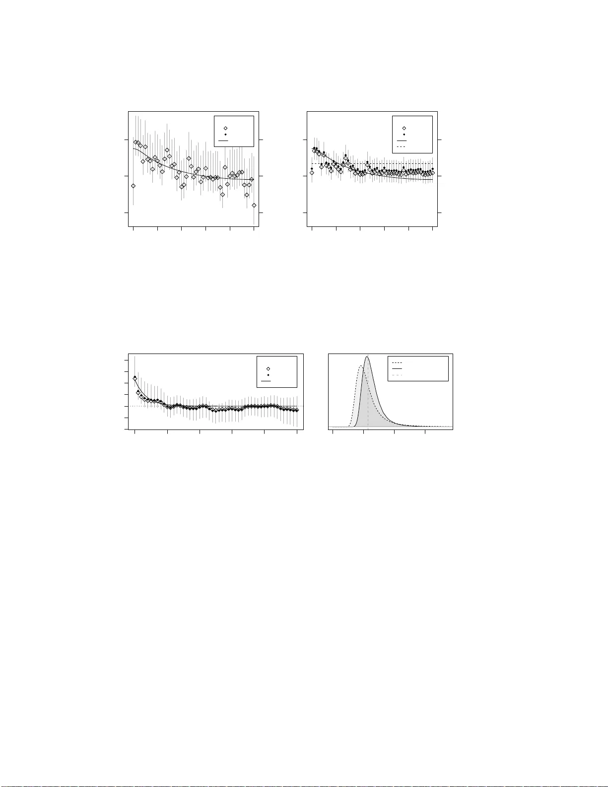
Original Paper
Loading high-quality paper...
Comments & Academic Discussion
Loading comments...
Leave a Comment