Adjusted Bayesian inference for selected parameters

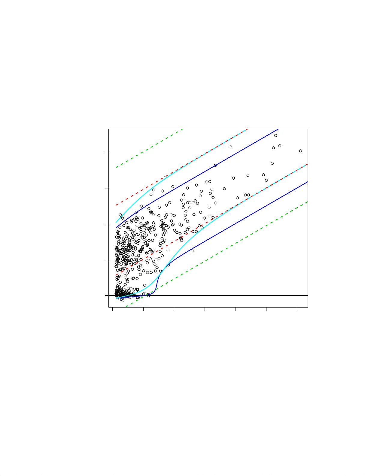
Adjusted Ba y esian inference for selected parameters Daniel Y ekutieli Octob er 29, 2018 Abstract W e address the problem of providing inference from a Ba yesian p er- sp ective for parameters selected after viewing th e data. W e presen t a Ba yesian framew ork for providing inference for selected parameters, based on the observ ation that providing Ba yesian in ference for selected param- eters is a truncated data p rob lem. W e sho w that if th e prior for the parameter is non-informative, or if the parameter is a “ﬁx ed” unkn o wn constant, then it is necessary to adjust the Ba yesian inference for selection. Our second contribution is the introduction of Ba yesian F alse Disco very Rate controlling metho dology , which generalizes existing Ba yesia n FDR metho d s that are only deﬁned in the tw o-group mixture model. W e il- lustrate our results by applying them to simulated data and d ata from a microarra y exp eriment. 1 In tro duction W e discuss providing Bayesian inference for par ameters s e le cted after viewing the data. Current thought is that selection has no aﬀect o n the inference of parameters from a B a yesian pers pective. W e show that this is not necess arily the case . Consider ge nerating a sample from a Bayesian fra mew ork by randomly generating the parameter and conditional on the para meter data are genera ted. In one cas e, selec tio n is applied to samples of the par ameter and the data, and in the other case the para meter is sampled and then sele c tion is applied to data samples. The exa mple b elow shows that selection ma tter s in the latter ca se, but not in the former case. Example 1.1 Let θ denote students’ true a cademic a bility . The marginal density of θ in the p opulation of high schoo l students is N (0 , 1). The o bserved academic ability of student s in high school is Y ∼ N ( θ, 1), and student s with 0 < Y a re admitted to colleg e. W e wish to predict a student’s true academic 1 ability from his obs erved academic ability – but only if the student is admitted to colle ge. W e will show that the Bayesian inference is diﬀer e nt fo r a r andom high school student than for a random co llege student . W e ﬁrst co nsider the case of a colleg e pr ofessor predicting θ for a student in his clas s. The joint distribution of ( θ , Y ) for a random colleg e studen t can b e generated by g enerating ( θ , y ) for a rando m high school student and selecting ( θ, y ) only if 0 < y . Thus the jo int density of ( θ, y ) us ed for predicting θ is f S ( θ, y ) ∝ e − θ 2 2 · e − ( θ − y ) 2 2 / Pr( Y > 0) ∝ e − ( θ − y/ 2) 2 2 · (1 / 2) , (1) and the conditional distribution of θ given Y = y is N ( y/ 2 , 1 / 2). The pr e dicted academic ability for a student with y = 1 is E ( θ | y = 1) = 0 . 5. F or the ca se of the high school tea c her predicting θ for a student in his class, we a ssume that there is a high scho ol regulation instr ucting tea chers to predict academic ability only for students that can b e a dmitted to college. This mea ns that for any true academic ability θ , the v alues of Y used to pr edict θ are dr a wn from the N ( θ, 1) density truncated by the even t 0 < Y . Since θ for a random student is N (0 , 1), the joint density of ( θ, y ) used for predicting θ is f S ( θ, y ) ∝ e − θ 2 2 · e − ( θ − y ) 2 2 / Pr( Y > 0 | θ ) . (2) In this case there is no closed ex pr ession for the conditional distribution of θ given Y = y , but since Pr( Y > 0 | θ ) decreases in θ then it is sto chastically smaller tha n N ( y/ 2 , 1 / 2), and the predicted academic a bilit y for a student with y = 1 is E ( θ | y = 1) = 0 . 1 0. In this pap er, we addres s selection that aris es in the statistical ana ly sis of large data sets in whic h the aim is to ﬁnd interesting parameters and then provide inferences for these selected pa rameters. Throughout the pa per we use the following simulated example to illustrate the discussio n. One can co nsider it a s an example of a microarr a y exp eriment in w hich θ i is the log-fold change in expression of Gene i and Y i is the observed log expres sion ratio. W e will now s ho w tha t even when the selection is applied to the par ameter and the data, it is necess ary to correct Bayesian inference for s election if the prior on the para meter is non-infor mativ e. Example 1 .2 The simulation includes 10 5 iid samples of ( θ i , Y i ). T o generate θ i , we ﬁrst sample λ i from { 1 0 , 1 } with proba bilities 0 . 90 and 0 . 10, a nd then 2 draw θ i from the lapla ce distr ibution, π 1 ( θ i | λ i ) = λ i · exp( − λ i · | θ i | ) / 2. Th us the marg ina l distribution o f θ i is π ( θ i ) = 0 . 9 · π 1 ( θ i | λ i = 10) + 0 . 1 · π 1 ( θ i | λ i = 1) . (3) Y i = θ i + ǫ i , with ǫ i independent N (0 , 1). In our analysis we apply the level q = 0 . 2 Benjamini and Ho ch b erg (1995) (hereafter BH) FDR controlling pro cedure to the tw o sided p-v alues, p i = 2 ∗ { 1 − Φ( | Y i | ) } , in or der to ﬁnd interesting θ i , and then co nstruct 0 . 95 credible int erv al for each interesting θ i . The BH pro cedure yielded R = 9 32 discov eries ( p (932) = 0 . 00 1862 < 0 . 0018 64 = 0 . 2 · 932 / 10 5 ): the s et of θ i with | Y i | > 3 . 111. The 932 selec ted ( θ i , Y i ) are display ed in Fig ure 1 . W e use tw o prior mo dels for constructing credible in terv als for θ i . In the ﬁrst mo del the prior distribution for θ i is π ( θ i ) in (3). In this case the p osterior distribution of θ i (w e der iv e it la ter in the pap er) is the conditiona l distribution of θ i given Y i . Thu s the probability that θ i is in the 0 . 95 cr e dible interv al constructed for it is, p er deﬁnition, 0 . 95. F urther more, s ince for eac h ( θ i , Y i ) we draw a new v alue of θ i from π ( θ i ), selection should have no aﬀect on the Bay esian inference. And indeed, 0 . 953 of the selected θ i (888 out of 932) are cov ered by their resp ective 0 . 9 5 cr e dible in terv als. In the second mo del we assume that the marginal distribution of θ i is un- known and we replace it with the non-informative prior, π ( θ i ) = 1 . The p osterio r distribution of θ i for this prior distribution is N ( Y i , 1). Th us Y i ± Z 1 − 0 . 05 / 2 is a 0 . 95 credible interv al for θ i (these ar e the red lines in Figur e 1). E ven though the po sterior distribution fo r non-informative priors is not the conditional distr ibu- tion of the para meter s given the data, these are equal tail credible interv als base d on minimally-informative prio r s known to pr o vide go o d freque ntist p erfor mance (Carlin and Louis, 1 996, Section 4 . 3) that a re exp ected to cover approximately 0 . 95 o f the θ i . These cr e dible interv als cov er 0 . 951 o f all 100 , 00 0 θ i , but only 0 . 654 of the se le cted θ i (610 out of 93 2). Before presenting o ur inferential framework in Sectio n 1.6, we re v iew a fre- quentist approach for discovering interesting para meters and pro viding infer- ences for these discoveries in Section 1.1. In s ection 1.2 we further motiv ate the impo rtance of o ur pr oblem b y reviewing literature on pr o viding inference for int eres ting par ameters in genomic s tudies . In Section 1.3- 1.5 several asp ects of Bay esian ana lysis that are relev ant to our w ork ar e reviewed. 3 1.1 Con trol ov er the false cov erage-statemen t rate Soric (198 9) asserted that the goal o f many scientiﬁc exp eriments is to discov er non-zero eﬀects, and as a result ma de the imp ortant o bserv ation that it is mainly the discov eries that are repo rted and included in to science, and warned that unless the prop ortion of fals e discov erie s in the set of declar ed discov eries is kept small there is da nger that a la r ge par t of science is unt rue. BH consider e d the pr oblem o f testing m n ull hyp o theses H 1 · · · H m , o f which m 0 are true null h yp otheses. They r eferred to the rejection o f a null hypothesis as a discovery and the rejection of a true null hypothesis as a false discov ery . T o limit the o c currence o f false discoveries when testing multiple null hypo theses BH in tro duced the F alse Discovery Rate F D R = E { V / max( R, 1) } , where R is the num b er o f discoveries and V is the num ber of false discov eries, and intro- duced the BH mu ltiple testing pro cedure that controls the FDR a t a no minal level q . Benjamini a nd Y ekutieli (200 5 ) gener alized the Benjamini and Ho ch b erg testing framework. In their selec tiv e inferenc e framework there are m parame- ters θ 1 · · · θ m , with c orresp onding estimators T 1 · · · T m , and the goa l is to con- struct v alid marg inal conﬁdence interv als (CIs ) for the subset o f para meters selected b y a given selection rule S ( t 1 · · · t m ) ⊆ { 1 · · · m } . They show ed that CIs cons tr ucted for sele c ted para meters no longer ensure the nominal cov er- age probability , and sugg ested the F alse Coverage-statement Ra te (F CR) a s the appropr iate criterio n to c a pture the error fo r CIs c o nstructed for selected parameters . The F CR is also deﬁned by E { V / max( R, 1 ) } , ho wev er R is the nu mber of CIs c o nstructed and V is the num ber of non- co vering CIs . Benja mini and Y ekutieli (2005) introduced a metho d of ensuring F C R ≤ q for indepe ndent T 1 · · · T m and a n y selection criterion: construct margina l 1 − R · q /m CIs for each of the R sele cted par ameters. In cases where each θ i can be asso ciated with a null v alue θ 0 i and the selection cr iteria are multiple testing pro cedures that test θ i = θ 0 i vs. θ i 6 = θ 0 i , Benjamini and Y ekutieli (2 005) show ed that the level q BH pro cedure can b e expressed a s the lea st conserv ative multiple test- ing pro cedure that ensures that all lev el q FCR adjusted CI fo r θ i , for which the null hypothes is is r ejected, will not c o ver the re spective θ 0 i . F urthermore, they show that for indep endent T 1 · · · T m if all θ i 6 = θ 0 i then applying the le v el q BH pro cedure to se le ct the parameter s and declar ing each se le c ted θ i greater than θ 0 i if T i > θ 0 i and smaller than θ 0 i if T i < θ 0 i controls the directional FDR (exp e c ted pr opo rtion o f selected parameters a ssigned the wrong sign) at lev el 4 q / 2. Example 1 .3 Note that in example 1.2 all θ i 6 = 0, th us for any multiple testing pro cedure F D R ≡ 0. How ever declar ing θ i po sitiv e for the BH dis co veries with Y i > 0 and neg ativ e for the BH discoveries with Y i < 0, ensur es directiona l- FDR less than 0 . 1 . The nu mber of simulated p ositive selected θ i with nega tiv e Y i and negative selected θ i with p ositive Y i is 56 , thus the obser v ed directional- FDR is 0 . 060. The r ed lines in Fig ure 1 are tw o-s ided Normal 0 . 95 CIs: Y i ± Z 1 − 0 . 05 / 2 (recall that these are also the non-info r mativ e pr io r 0 . 9 5 cr edible interv als from Example 1 .2). These 0 . 95 CIs co ver 95 , 08 9 of the 100 , 000 simulated θ i , but only 610 o f the 9 32 selected θ i , thus the obser v ed FCR is 0 . 346 . The green lines are 0 . 05 FCR-adjusted CIs: Y i ± Z 1 − 0 . 05 · 932 / (2 · 10 5 ) . The obs e rv ed FCR for the F CR-a djusted CIs is 0 . 046. 1.2 Selectiv e inference in Genomic asso ciation studies The need to co rrect inference for selection is widely reco gnized in Genome- wide asso ciation s tudies (GW AS). GW AS t ypically test as socia tion betw een a disease and h undreds o f tho us ands of markers lo cated throug ho ut the h uman genome, often expressed a s an o dds ratio o f manifesting the disease in carrier s of a risk allele. Only m ultiplicity-adjusted signiﬁca n t ﬁndings are repo rted. This limits the o ccurr e nce of fals e p ositives, howev er it in tro duces bias into the o dds ra tio es timates. Analyzing 301 published studies covering 25 diﬀerent rep orted as socia tions, Lo hm ueller et al. (2003) found that for 24 ass o ciatio ns the o dds ratio in the ﬁrst positive rep ort exceeded the genetic eﬀect es tima ted by meta-analy sis of the remaining studies. Zollner and Pritchard (2 0 07) sug g est correcting for the selection bias by providing p oint estimates a nd CIs based on the likeliho o d conditional on having o bserved a signiﬁcant asso ciation. Zhong and Pr e n tice (200 8) further a s sume that in the absence o f selection the log o dds ratio estimator is Normally distributed. Similarly to our Bay esian analysis of the simulated example, they base their inference o n a truncated nor mal conditiona l likelihoo d. 1.3 P arameter selection in Ba y esian analysis Berry and Ho c hberg (19 99) co mment that the Bay esian treatment of the multi- plicit y pro blem also includes decisio n ana lysis, r ather than just ﬁnding p o sterior 5 distributions. Scott and Berger (20 06) discuss Bayesian analy sis of microarr a y data. The prior mo del for θ i , the exp ectation of the log-fold change in expres s ion of Gene i , is that θ i = 0 with pro babilit y p a nd θ i ∼ N (0 , V ) with probability 1 − p . The decision analy sis per formed in Scott a nd Berger (2006) is the discovery of the subset of a ctiv e genes. Scott and Berger (20 06) decla re a g ene active ( θ i 6 = 0) if the p osterio r exp ected lo s s of this a ction is smaller than the p osterior exp ected loss of de c laring the gene inactive ( θ i = 0). The loss function for deciding that θ i = 0 is prop ortiona l to | θ i | , and the loss for erroneous ly deciding tha t θ i 6 = 0 is the ﬁxed cos t of doing a targeted exp eriment to verify that the g ene is in fac t active. The decision analy sis in Bayesian FDR a nalysis o f micr oarray da ta is als o deciding which genes are active. In Efro n et al. (200 1), θ i is selected if its lo cal FDR, which is the po sterior probability given y i that θ i = 0, is less than a nominal v alue q . Stor ey (20 02, 2003) sugg ests sp ecifying selection rules for which the p ositive FDR (pFDR), deﬁned a s the conditional probability that θ i = 0 given that θ i is selected, is less than q . In the optimal discov ery pro cedure suggested in Storey (20 07), the statistic used for s p ecifying the se le ction rule is a plug -in estimator of the lo cal FDR. Stor ey (2007) shows that the o ptima l discov ery pr ocedur e provides the max imal pro babilit y of selecting θ i among all selection rules with the same pFDR lev el. 1.4 Selection bias in B a yesia n analysis Dawid (199 4) explains why selection should hav e no eﬀect on B a yesian inference: “Since Bayesian pos ter ior distributions are already fully co nditioned on the data, the p osterior distribution o f any quantit y is the same, whether it was chosen in adv anc e or sele c ted in the light of the data.” Senn (200 8) reviews the disparity b e t ween Bay esian and freque ntist ap- proaches regar ding selection. He consider s the exa mple of providing inference for θ i ∗ , the eﬀect o f the phar maceutical as socia ted with the large s t sample mean y i ∗ , among a cla ss of m comp o unds with Y i ∼ N ( θ i , 4). He ﬁrs t shows that if θ i are iid N (0 , 1 ) the p osterior distr ibutio n of θ i ∗ is N ( y i ∗ / 5 , 4 / 5 ). He then assumes a hiera r c hical mo de l in which the trea tmen ts form a compo und c la ss. The class eﬀect is λ ∼ N (0 , 1 − γ 2 ) and θ i are iid N ( λ, γ 2 ). In this case he shows that the p osterior distributio n of θ i ∗ depe nds on the num b er of other comp ounds and their ov er a ll mean, howev er it is unaﬀected by the fact that θ i ∗ 6 was selected b ecause it c o rresp onds to the largest sample mea n. The observ atio n that Bayesian inference may b e aﬀected by selectio n was already made in Ma ndel and Rinott (20 07, 200 9 ). Mandel and Rinott (2007) consider the scenar io of providing inference for p , the probability of succes s in a binomial ex periment, co nditional on obs erving tw o or more suc c esses. Similar to Example 1.1, they distinguish betw een the case that in each binomial exp eriment p is drawn indep enden tly from its prior distribution a nd the case that the v a lue of p is the same in all binomial expe r imen ts, and they show that in the second case the Bay esia n inference is aﬀected by selec tio n. 1.5 Fixed and random eﬀects in Ba y esian analysis In the B a yesian framework there can b e no ﬁxed eﬀects since the parameters are reg arded as having pro babilit y distributions. How ever, discussing o ne-w ay classiﬁcation Box a nd T ia o (19 73, Section 7.2) use the sa mpling theory termi- nology of ﬁxed a nd ra ndo m eﬀects to distinguish be t ween situa tions in whic h the individual means can be r egarded as distinct v alues exp ected to bea r no strong relationship to e a c h other that can take on v alue s anywhere within a wide r ange, a nd situations in which the individual means ca n be rega rded a s draws fr o m a distributio n. Box and Tiao illustr ate this distinction with the example o f one-way classiﬁca tion of several g r oups of la bor atory yields. In the ﬁrst cas e the gro ups corresp ond to diﬀerent metho ds o f making a pa rticular chemical pro duct, while in the second case the g roups co rresp ond to diﬀerent batches made by the same metho d. The distinction only carr ies through to the prior mo del elicited for the gr oup mea ns. In the ﬁrst cas e the group means are elicited ﬂat no n-informative prior s. They call this mo del the ﬁxe d eﬀect mo del. In the second case the gr oup means are iid N ( λ, σ 2 ). This mo del is called the random eﬀect mo del. 1.6 Preliminary deﬁnitions Let θ denote the para meter, Y deno te the data and Ω is the sample space of Y . π ( θ ) is the pr ior distribution o f θ , and f ( y | θ ) is the likeliho o d function. The mult iple par ameters for whic h inference may o r may no t b e pr o vided, are actually multiple functions of θ : h 1 ( θ ) , h 2 ( θ ) , . . . . In selective inference fo r each h i ( θ ) there is a subset S i Ω ⊆ Ω, suc h that infer ence is provided for h i ( θ ) only if y ∈ S i Ω is observed. F or example, in our a nalysis of micro array data in Section 6, Y is the entire set of observed gene expression le vels; θ = ( σ 2 , µ ) consists 7 of the v arianc e s and exp ectations of the log-expres sion levels for a ll the g enes in the array; and infere nc e is provided for h g ( θ ) = µ g , the e x pectation of the log-fold c hange in express ion of Gene g = 1 · · · G , only if Gene g is decla red diﬀerentially expres sed by the BH pro cedure. Control over the FCR is a frequentist mechanism for providing selective in- ference. Notice that in E xample 1.2 a randomly se lected θ i is co vered b y its F CR-a djusted CI with pr obabilit y ≥ 0 . 95. But this frequentist selective infer- ence mechanism suﬀer s from several int rinsic limitations: it is impo ssible to incorp orate prior info r mation on the parameters ; it doe s not provide s election adjusted p oint estimates or selec tion-adjusted inference for functions of the pa- rameters; the selec tio n adjustment is the same rega rdless of the selection cr ite- rion a pplied and the v a lue of the e s timator. Figure 1 suggests that the selection adjustment ne e de d shrinks the CIs tow ard 0 , rather than just widening the CIs; and the the la rger | Y i | the smaller s election a djustmen t is needed for θ i . In selective inference the en tire data set Y = y is obser v ed. How ever, a s inference is provided for h i ( θ ) only if y ∈ S i Ω , then Y = y used for providing selective inference for h i ( θ ) is actually a realiza tion of the joint distribution of ( θ , Y ), trunca ted b y the even t that y ∈ S i Ω (describing Bayesian selec tive inference a trunca tion problem was sugg ested b y Br adley E fron in priv ate com- m unicatio n; for a discussion o n truncation see Mandel (20 07) and Gelman et al. (2004) Section 7.8). Th us in or der to provide Bay esian selective inference for h i ( θ ) w e intro duce a framework for providing Bay esia n infer ence bas ed on the truncated distribution of ( θ, Y ). W e call this inference selection-a djusted Bay esian (sa B a yes) inference Predicting true academic a bilit y fro m observed a cademic ability for a high school student and for a co llege student, discusse d in Exa mple 1.1, are Bayesian selective inference pro blems in which inference is provided for h ( θ ) = θ only if S Ω = { y : 0 < y } o ccurs. Notice that even though the selection mec hanism is diﬀerent, in b oth cas e s, ( θ , y ) fo r which θ is predicted from y are truncated samples from the distribution of ( θ , Y ) in the p opulation of all high schoo l student s. 1.7 Outline of the pap er In Section 2 w e discuss mo delling se lection-adjusted Bayesian inference: we provide an op erative deﬁnition fo r the joint truncated distr ibution of ( θ , Y ); we distinguish b e t ween par a meters a c cording to the wa y their distribution is 8 aﬀected by selection, and derive the joint truncated distribution of ( θ , Y ) in either cas e ; for either case, and a lso for parameter s with non-informa tiv e prior s , we deﬁne the components (i.e., prior, likelihoo d a nd p osterio r) o f s aBay es in- ference; we then sp eciﬁcally derive these c omponents for ( θ , Y ) that corres pond to Bo x and Tiao’s random eﬀect mo del and ﬁxed eﬀect mo del. In Section 3 we deﬁne sa Ba yes infer ence as the Bay es rules in Bay esian s e lectiv e inference. W e also present a Bayesian FCR fo r the random eﬀect mo del and explain the relation b et ween s aBay es inference and pr o viding FCR co n trol. In Section 4 we present Bayesian FDR controlling metho dology for spe c ifying selection rules in the random eﬀects mo del for cases in which s election is used for making statistical disc overies. W e also provide an eBayes alg orithm fo r ap- plying this metho dolog y in cases that co rresp ond to Box and Tiao’s ﬁxed eﬀect mo del. In Section 5 we explain the relatio n b e tween the Bay esia n FDR methods presented in Section 4 a nd e xisting Bayesian FDR metho ds, and des c ribe how to provide sa Bay es inference in the t wo g roup mixture mo del. In Section 6 we analyze microar ray da ta. The g oal of the analy sis is to ﬁnd ov er-expr e ssed and under -expressed genes while controlling directiona l FDR ≤ 0 . 0 5, a nd to pr o vide inference for the change in expressio n for thes e selected genes. The level 0 . 1 0 BH pro cedure applied to t statistic p-v alues fails to dis- cov er any diﬀere n tially ex pressed genes. Applying the level 0 . 1 0 B H pro cedure to p- v alues corresp onding to hybrid frequentist/eBay es mo derated t-statistics yields 245 discoveries, how e v er it is no t clear how to provide fr equen tist s elec- tive inference for these discov eries. F or compar ison, our level 0 . 05 Bay esian FDR selection r ule bas ed on the mo derated t-statistic yields 112 4 discov eries, and the level 0 . 05 Bayesian FDR se lection r ule based on the o ptimal statis tic yields 1 271 discov er ie s. In the second par t of the analysis, we pr o vide Bayesian selective inference for the exp ected log2-fold change in expres sion for a diﬀeren- tially expresse d g ene. The pap er concludes w ith a discussio n of the conc e ptual and metho do logical contributions of this pape r . 2 Mo delling selection-adjusted Ba y esian infer- ence The primary problem in mo delling saBay es inference is sp e cifying the join t truncated distribution o f ( θ, Y ), which we deno te f S ( θ, y ). It is imp ortant 9 to note that f S ( θ, y ) is the join t dis tribution of ( θ, Y ) acco rding to which se- lective inference is provided for h ( θ ), and not the jo int distribution of ( θ , Y ), f ( θ , Y ) = π ( θ ) · f ( y | θ ). W e use this characteriza tio n for deﬁning f S ( θ, y ). Deﬁnition 2.1 Assume that selective inference for h ( θ ) inv o lv es an action δ ( Y ) asso ciated with a loss function L ( h ( θ ) , δ ). f S ( θ, y ) is deﬁned as the distribution ov er which the exp ected loss r S ( δ ) = Z θ Z y ∈ S Ω f S ( θ, y ) · L ( h ( θ ) , δ ( y )) dy dθ (4) is the av era ge risk incurr e d in s electiv e inference for h ( θ ). 2.1 “Fixed,” “random,” and “mixed” parameters in Ba y esian selectiv e inference Example 1.1 illustrated that f S ( θ, y ) is determined by the wa y selection acts on θ . Unlike Box a nd Tia o who use the terms ﬁxed and random eﬀects to describ e the type of pr ior distribution elicited for θ , we use the terms “ﬁxed,” “rando m,” and “ mixed” parameters to describ e the wa y the distr ibutio n of θ is aﬀected by selection. F or each parameter type , w e der iv e f S ( θ, y ), π S ( θ ) the margina l truncated distribution of θ , and f S ( y | θ ) the truncated conditiona l distribution of Y | θ . 2.1.1 The “ﬁxed” parameter truncated sampl ing mo del W e call θ a “ﬁxed” pa rameter if its distribution is unaﬀected by selection and selection is a pplied to the co nditional dis tribution of Y given θ . ”Fixed” par am- eters a r e unknown constants whose v alues a re assumed to b e sampled from π ( θ ) and r e ma in unchanged. Th us fo r each v alue of θ , the ris k incurr ed in providing selective inference for h ( θ ) is the exp ected loss ov er the trunca ted conditiona l distribution of Y | θ Z y ∈ S Ω f ( y | θ ) /P r ( S Ω | θ ) · L ( h ( θ ) , δ ( y )) dy , for P r ( S Ω | θ ) = R y ∈ S Ω f ( y | θ ) dy , and the av era ge risk is its exp ectation ov er the marginal density of θ r S ( δ ) = Z θ Z y ∈ S Ω π ( θ ) · f ( y | θ ) /P r ( S Ω | θ ) · L ( h ( θ ) , δ ( y )) dy dθ . (5) 10 Thu s in this case the join t truncated distribution of ( θ , Y ) is f S ( θ, y ) = I S Ω ( y ) · π ( θ ) · f ( y | θ ) / Pr( S Ω | θ ) , (6) the marg ina l truncated density of θ is π S ( θ ) = π ( θ ) , (7) and the truncated conditional distribution of Y | θ is f S ( y | θ ) = I S Ω ( y ) · f ( y | θ ) / Pr( S Ω | θ ) . (8) 2.1.2 The “random” parameter truncated sampl ing mo del W e call θ a “ random” parameter in cases where selection is applied to the joint distribution o f ( θ, Y ). In this case θ is drawn from π ( θ ) and Y is drawn fro m f ( y | θ ), but inference is provided for h ( θ ) only for ( θ , y ) with y ∈ S Ω . Thus the av erage ris k incurred in providing s electiv e inference h ( θ ) is r S ( δ ) = Z θ Z y ∈ S Ω π ( θ ) · f ( y | θ ) /P r ( S Ω ) · L ( h ( θ ) , δ ( y )) dy dθ , (9) for P r ( S Ω ) = R θ R y ∈ S Ω π ( θ ) · f ( y | θ ) dy . Th us the truncated distribution of ( θ, Y ) is f S ( θ, y ) = I S Ω ( y ) · π ( θ ) · f ( y | θ ) / Pr( S Ω ) . (10 ) Int egr ating out y yields the mar g inal truncated distribution of θ π S ( θ ) = π ( θ ) · Pr( S Ω | θ ) / Pr( S Ω ) . (11) Dividing (10) b y (1 1) reveals that in this case the truncated distr ibution o f Y | θ is also the conditional likelihoo d in (8). 2.1.3 The “mixed” parameter truncated sampl ing mo del W e call θ a “mixed” parameter in cases wher e selection is applied to the con- ditional distribution of ( θ , Y ) given λ , for a hyperpa rameter λ ∼ π 2 ( λ ) with θ | λ ∼ π 1 ( θ | λ ). Th us conditioning on λ , θ is “random” and the av era g e risk incurred in pr o viding selective infere nce is Z θ Z y ∈ S Ω π 1 ( θ | λ ) · f ( y | θ ) /P r ( S Ω | λ ) · L ( h ( θ ) , δ ( y )) dy dθ , (12) 11 where P r ( S Ω | λ ) = R θ R y ∈ S Ω π 1 ( θ | λ ) · f ( y | θ ) dy dθ . T aking exp ectation over λ yields the average risk r S ( δ ) = Z λ Z θ Z y ∈ S Ω π 2 ( λ ) · π 1 ( θ | λ ) · f ( y | θ ) P r ( S Ω | λ ) · L ( h ( θ ) , δ ( y )) dy dθ dλ. (13) Thu s the truncated density o f ( λ, θ , y ) is f S ( λ, θ, y ) = I S Ω ( y ) · π 2 ( λ ) · π 1 ( θ | λ ) · f ( y | θ ) / Pr( S Ω | λ ) . (14) Changing the order of in tegr ation in (1 3 ) we get r S ( δ ) = Z θ Z y ∈ S Ω { Z λ π 2 ( λ ) · π 1 ( θ | λ ) P r ( S Ω | λ ) dλ } · f ( y | θ ) · L ( h ( θ ) , δ ( y )) dy dθ , (15) and thu s the truncated density of ( θ , y ) is f S ( θ, y ) = I S Ω ( y ) · f ( y | θ ) · Z λ π 2 ( λ ) · π 1 ( θ | λ ) / Pr( S Ω | λ ) dλ. (16) Int egr ating out y yields the mar g inal truncated distribution of θ π S ( θ ) = P r( S Ω | θ ) Z λ π 2 ( λ ) π 1 ( θ | λ ) Pr( S Ω | λ ) dλ. (17) And again, dividing (16) b y (17) r ev eals that the truncated distribution of Y | θ is f S ( y | θ ) in (8). Remark 2 .2 It is impo rtant to note that cla ssifying θ a “ﬁxed”, “r andom”, o r “mixed” parameter is co n text dep endent and must b e done on a case by case basis. In Example 1.1, θ is an unknown constant, for b oth a rando m c ollege student and a rando m high scho ol student . How ever, comparing Expr essions (1) and (2) with (6 ) and (10), reveals that θ is a “ ﬁxed” parameter fo r a random high school student, and a “ra ndom” para meter for a r andom college student. Senn’s example of providing inference for the most active comp ound ca n b e expressed as a selective inference problem in which, for i = 1 · · · m , inference is provided for h i ( θ ) = θ i only if S i Ω = { y : y i = max ( y 1 · · · y m ) } o ccurs. When θ is the vector o f treatment eﬀects of m distinct co mpounds, ea c h comp onent of θ is a distinct unknown co ns tan t whose v alue is sampled from N ( λ, γ 2 ) and remains unch ang ed, therefore θ is a “ﬁxed” parameter. Now supp ose that θ i ∼ N ( λ, γ i ) are batch eﬀects of m batches treated by a single comp ound, with comp ound eﬀect λ ∼ N (0 , 1 − γ 2 ). In this case, λ is a “ﬁxe d” unknown constant, and conditional on λ , θ is a “ra ndom” batch eﬀect. Thus θ is a “mixed” parameter. 12 2.2 Deﬁning the comp onen ts of Bay esian selective infer- ence The selection-adjusted prior distribution is, when it is av aila ble , the ma rginal truncated distribution of θ . W e have shown that the selection a djusted prior distribution for “ ﬁxed”, “random” o r “mixed” θ is π S ( θ ) giv en in (7), (11) or (17). Note that to s pecify the marginal truncated distr ibution o f θ , we need π ( θ ) to b e the marginal distribution of θ and we need to know how se le c tion acts on θ . An imp ortant case in which π ( θ ) is not the marg inal distributio n o f θ is when π ( θ ) is a non-informative prio r distribution. Non-informative pr iors are used to allow co nditional ana lysis on θ when no prior information on θ is av aila ble (Berger 198 5, Section 3 .3.1). As Y also provides all the infor mation on θ in the truncated data problem, we arg ue that the prio r distribution used for sa Bay es inference sho uld also b e a no n-informative prio r. W e further ar gue that while the lack of prior knowledge o n θ may aﬀect o ur decisio n to provide selectiv e inference, the opp osite is not true – the decis ion to provide infer e nc e o nly for certain v alues o f Y should hav e no eﬀect on the non-infor mativ e prior elic ited for θ . W e therefor e sug gest using the same non- informative prior for sa Bay es inference, π S ( θ ) = π ( θ ). Which means that if the prior for θ is non-informative then it is trea ted as a “ﬁxed” par ameter. The selection adjusted likelihoo d is f S ( y | θ ) in (8), the truncated conditiona l distribution of Y given θ . No te that conditioning o n θ ensur es that the sele c tion adjusted likelihoo d is the sa me in the thre e tr uncated sa mpling mo dels and do es not dep e nd on the marginal distribution of θ . The selection- adjusted p osterior distributio n is deﬁned by π S ( θ | y ) = π S ( θ ) · f S ( y | θ ) /m S ( y ) , (18) for m S ( y ) = R π S ( θ ) · f S ( y | θ ) dθ . F o r no n-informative priors it is g enerated by up dating the non-informa tiv e pr ior according to the selec tio n-adjusted like- liho od. F or “ﬁxed”, “random” or “mixed” θ it is the truncated co nditional distribution of θ | Y . Thus π S ( θ | y ) ∝ f S ( θ, y ). But no te that only for “r andom” θ , for which f S ( θ, y ) ∝ f ( θ, y ), the selection-adjusted p osterior distribution is unaﬀected by selectio n. Remark 2. 3 Dawid ar gues that s election has no e ﬀect on p osterior distri- butions since conditioning on the selection event is made redunda n t by condi- tioning on Y = y . Note that this only a pplies for the case of “random” θ , for 13 which s election ca n b e expr essed as co nditioning on an even t S in the sample space o f ( θ , Y ). Hence, as Dawid a rgues, for ( θ , y ) ∈ S the trunca ted p osterior distribution is the same as the untruncated p osterior distribution: π S ( θ | y ) = π ( θ | S, Y = y ) = f ( θ , S, Y = y ) f ( S, Y = y ) = f ( θ , Y = y ) f ( Y = y ) = π ( θ | Y = y ) = π ( θ | y ) . Whereas for “ﬁxed” a nd “mixed” θ , for which sele c tion cannot genera lly b e expressed as conditioning on an even t in the sample space of ( θ , Y ), π S ( θ | y ) is generally diﬀerent than π ( θ | y ) as demonstra ted in Exa mple 1 .1 and in E xample 2.4. W e illustr ate how this p oin t applies to our simulated data in Example 2.5. Example 2.4 Senn (20 08) concludes that selection has no eﬀect on the Bay esian inference beca use in his analys is θ is a “random” pa rameter. In Remark 2.2 we sug gest that in this kind o f analysis θ will most likely b e a “ﬁxed” or a “ mixed” par ameter. W e therefore compute the selection-adjusted po sterior mean of h 2 ( θ ) = θ 2 for m = 2 and y = (0 , 2), for “mixed” and “ﬁxed” θ . How ever, as S 2 Ω = { ( θ , y ) : y 2 ≥ y 1 } , then Pr( S 2 Ω | λ ) ≡ Pr( S 2 Ω ) = 0 . 5, and the “mixed” pa rameter mo del truncated jo in t de ns it y deﬁned in (16) reduces to the “random” parameter joint density in (10). Th us in this case , a lso fo r “ mixed” θ , the c onditional distribution of θ 2 is unaﬀected by selection. W e use Ex pr ession (4) in Senn (2 008) to compute the conditional mean of θ 2 . F o r γ 2 = 1 it equals 0 . 4 and for γ 2 = 0 . 5 it eq uals 0 . 384. The selection- adjusted joint density of θ for “ﬁxed” θ is g iv en by π S ( θ 1 , θ 2 | y = (0 , 2)) ∝ e − λ 2 2 γ 2 · e − ( θ 1 − λ ) 2 2 · (1 − γ 2 ) · e − ( θ 2 − λ ) 2 2 · (1 − γ 2 ) · e − (0 − θ 1 ) 2 2 · 4 · e − (2 − θ 2 ) 2 2 · 4 P r ( Y 2 ≥ Y 1 | θ 1 , θ 2 ) . In this cas e the selection adjustmen t increases the p osterio r distribution of θ v alues with θ 2 < θ 1 , thereby sto chastically decr easing the marg inal p osterior distribution of θ 2 . F or γ 2 = 1 the conditional mean o f θ 2 is 0 . 16 4 and for γ 2 = 0 . 5 it is 0 . 257 . 2.3 Mo deling Ba y esian selectiv e inference in the random eﬀect mo del Using the terminolog y sugge sted by Box and Tiao, w e call the mo del for θ = ( θ 1 · · · θ m ) a nd Y = { Y 1 · · · Y m } , where θ i are iid π ( θ i ) a nd Y i | θ i are independent f ( y i | θ i ), a ra ndo m eﬀect mo del. 14 In the random eﬀect mo del θ can b e a “ra ndom” pa rameter, a “ﬁxed” pa- rameter, a nd even a “mixed” parameter when there are iid “ﬁxed” λ i for which θ i | λ i are independent “ random” para meters. In any case the joint distribution of ( θ, Y ) is f ( θ , y ) = π ( θ ) · f ( y | θ ) = Π m i =1 π ( θ i ) · Π m i =1 f ( y i | θ i ) . (19) In selective inference for h i ( θ ) = θ i with S i Ω = { y : y i ∈ S mar g } , incorp orating (19) into (6) y ie lds the “ﬁxed” θ selection a djusted join t distribution of ( θ , Y ) f S ( θ, y ) = I S i Ω ( y ) · Π m j =1 { π ( θ j ) · f ( y j | θ j ) } / Pr( S i Ω | θ ) = Π j 6 = i { π ( θ j ) f ( y j | θ j ) } I S marg ( y i ) π ( θ i ) f ( y i | θ i ) / Pr( Y i ∈ S mar g | θ i ) . (20) Int egr ating out θ ( i ) and y ( i ) in (20) yields the selection adjusted distribution of ( θ i , Y i ) for “ﬁxe d” θ f S ( θ i , y i ) = I S marg ( y i ) · π ( θ i ) · f ( y i | θ i ) / Pr( Y i ∈ S mar g | θ i ) . (21) Similarly , incor pora ting (19) into (10) and integrating out θ ( i ) and y ( i ) , yields the selection adjusted joint distribution of ( θ i , Y i ) for “r andom” θ f S ( θ i , y i ) = I S marg ( y i ) · π ( θ i ) · f ( y i | θ i ) / Pr( Y i ∈ S mar g ) . (22) Incorp orating (19) into (16) and in tegr ating out θ ( i ) and y ( i ) , yields the “mixed” θ selection adjusted distribution of ( θ i , Y i ) f S ( θ i , y i ) = I S marg ( y i ) · f ( y i | θ i ) · Z π 2 ( λ i ) · π 1 ( θ i | λ i ) Pr( Y i ∈ S mar g | λ i ) dλ i . (23) 2.3.1 The non-exc hangeable random eﬀect mo del The no n- exc hange a ble random eﬀect mo del is a generaliza tion of the random eﬀect mo del for situations in which θ i are distinct v alues exp ected to b ear no strong relationship one to each other, i.e. s ituations for whic h B o x a nd Tiao would suggest the ﬁxed eﬀect mo del. In the non-e x c hangea ble ra ndom eﬀect mo del θ i are indep endent but hav e dis tinct prior distributions, π i ( θ i ), while Y i | θ i are still indep enden t f ( y i | θ i ). Thus the joint distribution of ( θ , Y ) is f ( θ , y ) = π ( θ ) · f ( y | θ ) = Π m i =1 π i ( θ i ) · Π m i =1 f ( y i | θ i ) . (24) The marginal distr ibution of ( θ i , Y i ) is f ( θ i , y i ) = π i ( θ i ) · f ( y i | θ i ) . 15 But in selective inference for h i ( θ ) = θ i with S i Ω = { y : y i ∈ S mar g } , the selection adjusted joint dis tribution of ( θ i , Y i ) for “ﬁxe d” θ is f S ( θ i , y i ) = I S marg ( y i ) · π i ( θ i ) · f ( y i | θ i ) / Pr( Y i ∈ S mar g | θ i ) . (25 ) Example 2.5 Notice that ( θ , Y ) in Example 1.2 ar e generated b y the r an- dom eﬀect mo del that the comp onents of θ = ( θ 1 · · · θ 100 , 000 ) are indepe ndently drawn from π ( θ i ) in (3) and Y i | θ i are independent f ( y i | θ i ) = φ ( y i − θ i ). Fig- ure 1 is a scatter plo t of 932 ( θ i , y i ) with | y i | > 3 . 111; Figur e 4 displays the 470 comp onents with y i > 3 . 111. F o r compar ison, in the comparable non- exchangeable rando m eﬀect mo del: for i = 1 · · · 9 0 , 000, θ i ∼ π 1 ( θ i | λ i = 10 ) and for i = 9 0 , 001 · · · 100 , 00 0, θ i ∼ π 1 ( θ i | λ i = 1). It is imp ortant to note that in Ex a mple 1.2 we draw a single rea lization from the joint untruncated dis tribution of ( θ , Y ). T o obs e rv e the diﬀerence b et ween “random” , “ﬁxed” and “ mixed” θ w e conduct a no ther set of simulations, in which we sample 100 0 realizations of ( θ , Y ) from its truncated distributions for h 1 ( θ ) = θ 1 with S 1 Ω = { y : | y 1 | > 3 . 1 11 } fo r “random”, “ﬁxed” and “mixed” θ . E ac h realization from the “ra ndom” θ trunca ted distribution is generated by r epeatedly sa mpling ( θ, Y ) from its un truncated distribution, keeping the ﬁrst ( θ , y ) for which | y 1 | > 3 . 111. T o ge ne r ate each realization from the “ﬁxe d” θ truncated distributio n, we sample θ fro m π ( θ ) and then rep e atedly sample Y , keeping the ﬁrst y with | y 1 | > 3 . 111 . As the comp onen ts of ( θ , Y ) are independent the distribution of ( θ 2 , · · · , θ 100 , 000 , Y 2 , · · · , Y 100 , 000 ) is the sa me in the thr e e trunca tion mo dels. Figure 2 displays the scatter plo ts of the Y 1 > 3 . 1 11 realizations of ( θ 1 , Y 1 ) for each truncation mo del. The left panel is the sc a tter plot for the “ra ndom” θ model. In this ca se the joint density of ( θ 1 , Y 1 ), given in (22), is π ( θ 1 ) · φ ( y 1 − θ 1 ) , and it is identical to the joint dens it y of ( θ i , Y i ) display ed in Figures 4 and the distribution of ( θ i , Y i ) fo r Y i > 3 . 1 11 in Figure 1. The right panel is the scatter plot for the “ ﬁxed” θ mo del. In this cas e the joint density of ( θ 1 , Y 1 ), given in (21), is π ( θ 1 ) · φ ( y 1 − θ 1 ) / Pr( | Y 1 | > 3 . 111 | θ 1 ) . Comparing the right and left panels reveals tha t in this mo del, for each v alue of Y 1 , the conditional distribution θ 1 is shrunk tow ards 0. T o gener ate eac h realization from the “mixed” θ truncated distribution, for i = 1 · · · 10 0 , 000 we 16 independently sample λ i from { 10 , 1 } , with pr obabilities 0 . 9 0 a nd 0 . 10, and then we rep eatedly sample ( θ , Y ), θ i ∼ π 1 ( θ i | λ i ) and Y i ∼ φ ( θ i ), keeping the ﬁrst ( θ, y ) for which | y 1 | > 3 . 111. The joint density of ( θ 1 , Y 1 ) given in (23) is { 0 . 9 · π 1 ( θ 1 | λ 1 = 10 ) Pr( | Y 1 | > 3 . 111 | λ 1 = 10) + 0 . 1 · π 1 ( θ 1 | λ 1 = 1) Pr( | Y 1 | > 3 . 111 | λ 1 = 1) } · φ ( y 1 − θ 1 ) . Comparing the three panels of Figure 2 r ev eals that in this mo del the shrinking of the distribution of θ 1 | Y 1 = y 1 tow ards 0 is weaker than in the “ﬁxed” θ mo del. 3 Selection-adjusted Ba ye sian inference T o deﬁne saBayes inference, w e express the av er a ge risk incurr ed by providing selective inference for h ( θ ) r S ( δ ) = Z θ Z y ∈ S Ω L ( h ( θ ) , δ ( y )) · π S ( θ ) · f S ( y | θ ) dy dθ = Z y ∈ S Ω [ Z θ L ( h ( θ ) , δ ( y )) · π S ( θ | y ) dθ ] · m S ( y ) dy . (26) Thu s the Bayes rules in s electiv e inference are the actio ns minimizing the selection- adjusted p osterior exp ected loss ρ S ( δ, y ) = Z L ( h ( θ ) , δ ( y )) · π S ( θ | y ) dθ , and in general Bay esian selective inference s ho uld be based o n the sele ction- adjusted p osterio r distribution of h ( θ ), π S ( h ( θ ) | y ). Selection-adjusted 1 − α credible int erv als for h ( θ ) are subsets A for which Pr π S ( h ( θ ) | y ) ( h ( θ ) ∈ A ) = 1 − α , and the p osterior mean or mo de of π S ( h ( θ ) | y ) can ser v e as selection-adjusted po in t estimato rs for h ( θ ). Example 3 .1 W e provide saBay es infer ence for the data simulated in Example 1.2 for t wo se le cted para meter s: h 12647 ( θ ) = θ 12647 with S 12647 Ω = { y : | y 12647 | > 3 . 111 } , and h 90543 ( θ ) = θ 90543 with S 90543 Ω = { y : | y 90543 | > 3 . 111 } . Since we hav e drawn θ from π ( θ ) a nd Y from f ( y | θ ) then θ is a “ random” pa rameter. Recall that w e use tw o prior models for θ in our analys is . In the ﬁrst mo del we as s ume that ( θ , Y ) w as gener ated by a random eﬀect mo del with π ( θ i ) in (3). In this mo del the sa B a yes p osterio r distribution of θ i is pr opo rtional to the distribution of ( θ i , Y i ) in (22) π S ( θ i | y i ) ∝ π ( θ i ) · φ ( y i − θ i ) . (27) 17 In the second model ( θ , Y ) is g enerated by a non- e x c hangea ble random eﬀect mo del with unkno wn π i ( θ i ) (note that if it were assumed that θ was gener ated by a r andom eﬀect mo del then eBay es co uld be used to estimate π ( θ i )). Thus, following Box and Tia o, we use the ﬂat non-informa tiv e pr ior π i ( θ i ) = 1 in our analysis. The ﬂat prior unadjusted p osterior distribution of θ i is π ( θ i | y i ) ∝ φ ( y i − θ i ) . (28) The non-informa tiv e prior sa Ba yes p osterior distr ibution of θ i is prop ortiona l to the distribution of ( θ i , Y i ) for “ﬁxe d” θ in (21) π S ( θ i | y i ) ∝ φ ( y i − θ i ) /P r ( S mar g | θ i ) , (29) with P r ( S mar g | θ i ) = Φ( − 3 . 111 − θ i ) + 1 − Φ(3 . 111 − θ i ). Figure 3 displays the p osterio r distributions of θ 12647 (left pane l) and θ 90543 (right panel). The ﬂat pr ior unadjusted p osterior mean and mo de of θ 12647 equal Y 12647 = 3 . 4 0, and the 0 . 95 credible interv al is [1 . 44 , 5 . 36]. The saBay es po sterior distribution of θ 12647 is shrunk towards 0. The “rando m” θ sa Ba yes po sterior distr ibution of θ 12647 is bimo dal with a s pik e at 0 and a mo de at 2 . 40, the p osterior mean is 1 . 68, and the 0 . 95 cr edible interv al is [ − 0 . 11 , 4 . 20]. The ﬂat prio r saBay es p osterior mo de of θ 12647 is 0 . 74, the p osterior mea n is 1 . 88, and the 0 . 95 cr e dible int er v al is [ − 0 . 04 , 4 . 64]. The ﬂat prior unadjusted p osterior mean and mo de o f θ 90543 equal Y 90543 = 5 . 59, and the 0 . 95 cr edible in terv al is [3 . 63 , 7 . 5 5]. The m uch la rger Y 90543 pro- duces a no n-negligible likelihoo d o nly for θ i v alues that corr e spond to a lmost certain selection. Thus in this case the selectio n adjustment is small: the ﬂat prior sa Bay es p osterior mode is 5 . 57, the p osterior mean is 5 . 4 8, and the 0 . 95 credible interv al is [3 . 26 , 7 . 52 ]. The shrinking tow ards 0 in the “rando m” θ mo del p osterio r is stro ng er: the p osterior mean and mo de are 4 . 59 and the 0 . 95 credible interv al is [2 . 62 , 6 . 55]. Remark 3. 2 It is imp ortant to note that as extremely unlikely v alues o f θ with an extremely small selection proba bilit y ca n have a large selection-adjusted like- liho od, the selection a djustment p osterior distribution ca n b e b e v ery diﬀerent than the unadjusted pos terior distribution. The selection-a djusted likeliho od can even be non-informative and improp er – if the se le ction rule o nly includes the o bserved v a lue Y = y then the selectio n-adjusted likelihoo d is co nstan t fo r all pa r ameter v a lues. Example 3 .3 illustrates this phenomenon, shows how it is 18 aﬀected by the choice of the selection rule a nd that it is not unique to Bayesian selective inference. In this pap er we employ selection rules who se selection prob- ability is minimized a t θ = 0 and approa c hes 1 for la r ge | θ | , thus the selection adjustment s shrink the likeliho o d tow ar ds 0. Example 3. 3 W e derive the no n-informative prior s aBay es p osterior dis- tribution o f θ 12647 , given in (29), for an alternative o ne-sided selectio n rule S 12647 Ω = { y : y 12647 > 3 . 111 } . In this cas e the s e lection-adjusted p osterio r is sto c hastica lly smaller and muc h more diﬀuse. The selec tion-adjusted p os- terior mo de is 0 . 19 and the selection-adjusted p osterior mean is − 2 . 8 7; the 0 . 95 selection- a djusted cr edible in terv al is [ − 15 . 41 , 3 . 91 ]. An unlikely v alue θ 12647 = − 5 . 87, with unadjusted likelihoo d φ ( − 5 . 87 − 3 . 40) = 8 . 73 × 10 − 20 and selection probability Φ( − 5 . 87 − 3 . 11 1) = 1 . 34 × 10 − 19 , has the same selection- adjusted p osterior densit y as the unadjusted p osterior mode θ 12647 = 3 . 40, i.e. π S ( θ 12647 = − 5 . 87 | Y 12647 = 3 . 40) = π S ( θ 12647 = 3 . 4 0 | Y 12647 = 3 . 4 0). W e now show that frequentist selection adjusted inference can also be very diﬀerent than the unadjusted freq uen tist inference, and highly de p endent on the type of selection rule used. The ﬂat pr ior unadjusted 0 . 95 credible interv al for θ 12647 , [1 . 4 4 , 5 . 36] is also a 0 . 95 frequentist co nﬁdence interv al for θ 12647 . T o construct sele c tion-adjusted fr e q uen tist 0 . 95 c onﬁdence int er v als for θ 12647 we beg in by testing, at level 0 . 05 a nd for each v alue of θ 0 , the null hyp o thesis that θ 12647 = θ 0 . The sampling distr ibution of Y 12647 | θ 12647 = θ 0 is f S ( y 12647 | θ 12647 ) in (8) with θ 12647 = θ 0 . Thus we reject the null hypothesis that θ 12647 = θ 0 if y 12647 is smaller than the 0 . 025 quantile or larger than the 0 . 97 5 qua n tile of f S ( y 12647 | θ 0 ), and the 0 . 95 conﬁdence in terv al for θ 12647 is the set of θ 0 v alues for which the null hypo thesis that θ 12647 = θ 0 is not r ejected for y 12647 = 3 . 4 0. F or the selec tio n rule S 12647 Ω = { y : | y 12647 | > 3 . 111 } the 0 . 95 conﬁdence in terv al for θ 12647 is [ − 0 . 37 , 5 . 03]. While for S 12647 Ω = { y : y 12647 > 3 . 111 } the 0 . 95 conﬁdence interv al for θ 12647 is [ − 9 . 44 , 5 . 03]. 3.1 F CR control in the random eﬀect mo del W e deﬁne the FCR for ( θ , Y ) gener ated by the random eﬀect mo del. The initial set of par ameters is θ 1 · · · θ m . The subset o f s elected parameters is { θ i : y i ∈ S mar g } , and a margina l conﬁdence in terv al A mar g ( y i ) is constructed for ea c h selected θ i . F o r i = 1 · · · m , let R i = I ( Y i ∈ S mar g ) and V i = I ( Y i ∈ S mar g , θ i / ∈ 19 A mar g ( Y i )). R = P R i is the num b er of selected par ameters, V = P V i is the nu mber of non-co vering conﬁdence interv als, and F C P = V /max (1 , R ) is the false co verage-statement prop ortion. In Benjamini and Y ekutieli (2005) FCR refers to a frequentist FCR that corresp onds to E Y | θ F C P for ( θ , Y ) generated by a random eﬀect mo del. In this pap er FCR is a Bayesian FCR, deﬁned by E θ ,Y F C P . W e a lso cons ide r the p ositive FCR, pF C R = E θ ,Y ( F C P | R > 0). 3.1.1 Relation b etw e e n F CR con trol and Bay esi an se lectiv e infer- ence Note that fo r i = 1 · · · m , the indicators R i and V i are de ﬁned for the joint (un truncated) distributio n of ( θ , Y ). The even t R i = 1 is given by { ( θ , y ) : y i ∈ S mar g } . The conditio nal distr ibution of ( θ, Y ) given R i = 1 is f ( θ , y | R i = 1) = I S marg ( y i ) · Π m j =1 { π ( θ j ) · f ( y j | θ j ) } / Pr( Y i ∈ S mar g ) , (30) and integrating o ut θ ( i ) and y ( i ) yields the conditional distribution of ( θ i , Y i ) given R i = 1 to be f ( θ i , y i | R i = 1) = I S marg ( y i ) · π ( θ i ) · f ( y i | θ i ) / Pr( Y i ∈ S mar g ) . (31) This is the sa me as the “ra ndom” para meter selection-a djusted distribution of ( θ i , Y i ) g iv en in (22). This implies that the conditiona l probability that the conﬁdence interv al co nstructed for θ i fails to cov er θ i , given that θ i is selected, can b e expr essed as the av erage r isk incurr ed in s electiv e inference for h i ( θ ) = θ i with S i Ω = { y : y i ∈ S mar g } a nd with θ being a “ra ndom” para meter, for the loss function L ( θ i , A i ( y )) = I ( θ i / ∈ A mar g ( y i )): Pr( V i = 1 | R i = 1) = Z θ i Z y i ∈ S marg π ( θ i ) f ( y i | θ i ) · I ( θ i / ∈ A mar g ( y i )) Pr( Y i ∈ S mar g ) dy i dθ i = r S . (32) Pr( V i = 1 | R i = 1 , Y i = y i ) is equal to the “ra ndom” θ selection adjusted po sterior exp ected loss ρ ( y i ) = Z I ( θ i / ∈ A mar g ( y i )) · π S ( θ i | y i ) dθ i , (33) for π S ( θ i | y i ) ∝ π ( θ i ) · f ( y i | θ i ) the “ random” θ s e lection adjusted p osterior dis- tribution. Prop osition 3. 4 The pFCR and E V /E R ar e e qual to the “ r andom” θ aver- age risk in (32) . If A mar g ( y i ) ar e 1 − α cr e dible intervals for θ i b ase d on t he “r andom” θ sele ction adjuste d p osterior distribution then p F C R = α . 20 Pr o of. In the random eﬀect mo del { V i : R i = 1 } a re mutually indep endent with Pr( V i = 1 | R i = 1) = r S . Th us for each v alue of R = k , V ∼ B inom ( k , r S ), and conditioning on R > 0 yields pF C R = r S . Note that the numerator and denominator in (32) eq ua l E V i and E R i . Thus E V / E R = E V i /E R i is also r S . Lastly , for 1 − α selection-a djusted cr e dible interv als based on π S ( θ i | y i ), r S = ρ ( y i ) ≡ α . ¶ Remark 3 .5 W e hav e shown tha t in the random eﬀect model, regardless of whether θ is “r andom”, “ﬁxed” or “mixed” , the pFCR equals the “random” θ sele ction-adjusted average risk. As pFCR ≥ Bay esian- F CR the “random” θ av erage risk can s erve as a cons erv ative estimate for Bay esian-FCR. In par ticu- lar, for la rge R the sampling disp ersion o f FCP and of V /E R is small, th us the F CP , Bayesian-F CR, frequentist-F CR, and pFCR that equals E V /E R , which we discuss in the context of sp ecifying selection rules in the non-exchangeable random eﬀect mo del, are a lmost the same. Remark 3.6 Recall that if π ( θ i ) is a no ninformative prio r then the selectio n adjusted p osterior distribution for “rando m” θ is deﬁned π S ( θ i | y i ) ∝ π ( θ i ) · f ( y i | θ i ) / Pr( S mar g | θ i ) . (34) As cr edible in terv als ba sed on non-infor mativ e pr iors are exp ected to provide approximate cov era ge probability , when π ( θ i ) is a non-infor mativ e prior then 1 − α credible interv als based on π S ( θ i | y i ) in (34) yield ρ ( y i ) ≈ α . Thus P rop osition 3.4 implies that for non informa tiv e priors the “ﬁxed” θ mar ginal 1 − α credible int erv als yield a ppr o ximate level α F CR co n trol. Example 3.7 Figure 4 displays ( θ i , y i ) gener ated in Example 1.2 with y i > 3 . 111. The red and gree n dashed curves ar e the 0 . 95 conﬁdence interv als fro m Figure 1. The red curves also corres pond to the 0 . 95 credible in terv als for θ i for the ﬂat prio r unadjusted p osterior (28). The blue curves ar e the 0 . 95 saB a yes credible interv als fo r the ﬂat prior selection-adjusted p osterio r in (29), and the light blue curves are the 0 . 95 saBayes credible interv als for the “ra ndom” θ selection-adjusted p osterior in (27). According to Prop osition 3.4 the pFCR for “r andom” θ 0 . 95 saBayes credible int erv als co nstructed for selected ( θ i , y i ) is 0 . 0 5. In E xample 1.2 we have seen 21 that the FCP for these credible interv als for the 93 2 se le c ted θ i was 0 . 04 7. As the ﬂat prio r unadjusted credible interv als are 0 . 9 5 frequentist conﬁdence interv als, we exp ect the cov era ge prop ortion for all 10 0 , 000 θ i to b e close to 0 . 95. W e hav e seen that these CIs cover 95 , 089 of the 100 , 000 θ i , but that the FCP for the 93 2 s e lected parameters is 0 . 346. Benjamini and Y ekutieli (2005) explain this pheno menon from a frequentist pe r spective. Remark 3.6 oﬀers a Bay esian explanation: in o rder to provide approximate FCR co n trol for non informative priors the credible interv als should b e ba sed on the “ﬁxed” θ selectio n adjusted po sterior in (29), rather than the “random” θ selection adjusted pos ter ior in (28). And indeed, the F CP o f the credible interv als based o n (2 9) is 0 . 040 . 4 Sp ecifying FDR con trolling selection rules in the random eﬀect mo del W e will now present Bayesian methodo logy for sp ecifying sele c tion rules in the random eﬀect mo del and the no n-exc hang eable random eﬀect mo del for ca ses in which selection is a pplied for making statistica l discov erie s. Similarly to the BH FDR con trolling appr oach, w e seek to control the pro portio n of false discov eries co mmitted. Unlik e BH, in which dis c o veries refer to r e jection of nu ll hypo theses a nd the statistics used for sp ecifying the selection rule ar e p- v alues testing these null hypo theses, in our approach any even t in the parameter space can b e co nsidered a discov er y and a n y statistic may b e used fo r spe c ifying the selection rule. But, as suggested in Stor ey (2007), w e will show that for any g iv en disco very the optimal statistic is the posterio r probability that the discov ery is false. As in Section 3 .1, w e a ssume that ( θ , Y ) are gener ated by the r andom eﬀect mo del; θ i is selected if y i ∈ S mar g ; and the inference pr o vided for θ i if it is selected is decla ring that θ i ∈ A mar g ( y i ). Ho wev er now A mar g ( y i ) is an even t that co rresp onds to mak ing a statistical disc overy r egarding θ i . F or example, in the microa rray analysis in Section 6, in which the discov ery is declaring a g e ne either ov er or under expressed, for y i > 0 the discovery even t is A mar g ( y i ) = { θ i : θ i > 0 } . Once decla r ing θ i ∈ A mar g ( y i ) co r resp onds to making a statistical discov ery , R b ecomes the num b er of discoveries, V b ecomes the num ber of false discoveries, V /max (1 , R ) = F D P is the fals e discov ery prop ortion, a nd F C R = F D R . Th us Prop osition 3.4 yields the following result. 22 Corollary 4. 1 In the r andom eﬀe ct mo del the pF D R e quals r S in (32 ) , which is the c onditional pr ob ability given t hat θ i is sele cte d t hat the disc overy r e gar ding θ i is fa lse, and ρ ( y i ) in (33) is the c onditional pr ob ability given sele ction and given Y i = y i that t he disc overy is false. Thu s in or de r to ens ur e level q FDR control, when conside r ing selection rules of the form S mar g = { y i : T ( y i ) ≤ s } , we sugg est cho osing s for which r S in (32) is ≤ q . F urthermo re, reexpressing r S r S = R y i ∈ S marg m ( y i ) · R θ i π S ( θ i | y i ) · I ( θ i / ∈ A mar g ( y i )) dθ i dy i Pr( Y i ∈ S mar g ) = R y i ∈ S marg m ( y i ) · ρ ( y i ) dy i R y i ∈ S marg m ( y i ) dy i (35) where m ( y i ) = R π ( θ i ) · f ( y i | θ i ) dθ i , yields the following Neyman-Pearson Lemma t yp e res ult, prese nted in Storey (200 7). Corollary 4. 2 The s ele ction rule of the form S mar g = { y i : ρ ( y i ) ≤ s } has the lar gest sele ction pr ob ability of al l sele ction rules with the same pFDR. Another option is to us e ρ ( y i ) to directly spe cify the s election r ule, by deﬁning S mar g = { y i : ρ ( y i ) ≤ q } . (36) Notice that unlike the contin uum of p ossible credible in terv als that can b e con- structed for θ i , the num b er o f p ossible discoveries tha t ca n b e made rega rding θ i is usually ﬁnite, e.g. discov ering that θ i is either negative or p ositive or dis- cov ering that θ i is the larg e s t comp onent in θ . In pa rticular, when there is only a sing le poss ible discov ery for all selected v a lue s of y i , i.e. A mar g ( y i ) ≡ A mar g , then express ing the “r andom” θ average risk corr esponding to this discov ery r S = Z Z y i ∈ S marg I ( θ i / ∈ A mar g ) · π ( θ i ) · f ( y i | θ i ) Pr( Y i ∈ S mar g ) dy i dθ i = Z I ( θ i / ∈ A mar g ) · π ( θ i ) Pr( Y i ∈ S mar g | θ i ) Pr( Y i ∈ S mar g ) dθ i = Z I ( θ i / ∈ A mar g ) · π S ( θ i ) dθ i , (37) for π S ( θ i ) = π ( θ i ) · Pr( S mar g | θ i ) / Pr( S mar g ) the “r a ndom” θ se le ction-adjusted prior density der iv ed in (11), yields the following res ult. Corollary 4. 3 If A mar g ( y i ) ≡ A mar g then the pF D R is e qual to the “ r andom” θ sele ction-adjuste d prior pr ob ability that θ i / ∈ A mar g . 23 4.1 Sp ecifying FDR controlling selection r ules in the non- exc hangeable random eﬀect mo del In this subsection, ( θ, Y ) is generated by the no n-exchangeable random eﬀect mo del, θ i is selected if y i ∈ S mar g , a nd the infere nce provided for selected θ i is the discovery that θ i ∈ A mar g ( y i ). Let A 1 mar g · · · A D mar g denote the D p ossible discov eries that ca n b e made on θ i . F or d = 1 · · · D , let R d denote the n umber of discov eries o f A d mar g and let V d denote the num b er of fals e discov eries of A d mar g . The r esults in this section a r e derived under the assumption that A mar g ( y i ) ≡ A mar g . How e v er as E R = E R 1 + · · · + E R D and E V = E V 1 + · · · + E V D , they can b e easily extended for the case of D > 1. T o derive the results in this section, we ass ume that there als o exists ( ˜ θ, ˜ Y ), generated by the random para meter mode l that ˜ θ i are iid ˜ π ( θ i ) = P m i =1 π i ( θ i ) /m , and ˜ Y i | ˜ θ i are indep enden t f ( ˜ y i | ˜ θ i ). Lemma 4. 4 F or any su bset B , W i = I ( y i ∈ S mar g , θ i / ∈ B ) , and ˜ W i = I ( ˜ y i ∈ S mar g , ˜ θ i / ∈ B ) E m X i =1 W i = E m X i =1 ˜ W i . Pr o of. E m X i =1 W i = m X i =1 Pr( Y i ∈ S mar g , θ i / ∈ B ) = m X i =1 Z θ i / ∈ B Z y i ∈ S marg π i ( θ i ) · f ( y i | θ i ) dy i dθ i = m X i =1 Z θ 1 / ∈ B Z y 1 ∈ S marg π i ( θ 1 ) · f ( y 1 | θ 1 ) dy 1 dθ 1 = m · Z θ 1 / ∈ B Z y 1 ∈ S marg m X i =1 π i ( θ 1 ) /m · f ( y 1 | θ 1 ) dy 1 dθ 1 = m · Z θ 1 / ∈ B Z y 1 ∈ S marg ˜ π ( θ 1 ) · f ( y 1 | θ 1 ) dy 1 dθ 1 = E m X i =1 ˜ W i ¶ Notice that for B = ∅ , P m i =1 W i is the num b er o f discoveries R . While for B = A mar g , P m i =1 W i is the n umber of false discov eries . Therefore Lemma 4.4 implies that E V , E R , thus a lso pF D R = E V / E R , for ( θ, Y ) a nd for ( ˜ θ, ˜ Y ) ar e 24 the same. According to Coro lla ry 4.1 the pF D R for ( ˜ θ , ˜ Y ) is the cor respo nding “random” θ av erag e ris k, w e denote ˜ r S . Th us s inc e F D R ≤ pF DR , and pF D R is the same for ( θ, Y ) and for ( ˜ θ, ˜ Y ), w e get the following result. Corollary 4. 5 In the non-ex change able r andom p ar ameter m o del sele cting θ i if y i ∈ S mar g yields level ˜ r S F D R c ontro l. T o deﬁne a genera l metho d for sp ecifying FDR co n trolling sele ction rules for ( θ, Y ) generated by the non-exchangeable random eﬀect mo del with unknown marginal prior s , notice that applying empir ical Bay es metho ds to y 1 · · · y m actually estimates ˜ π ( θ i ), the mixture of the (unknown) mar ginal densities of θ 1 · · · θ m . Co m bining this with Cor ollary 4.5 implies that the FDR of any se - lection rule ca n be approximated b y ˜ r S computed by trea ting ( θ , Y ) as if it was generated by the r andom eﬀect mo del and using the eBay es estimate of ˜ π ( θ i ). F urthermo re, as E R = E ˜ R and E ˜ R = m · Pr( ˜ Y i ∈ S mar g ), then also in the non- exchangeable rando m eﬀect mo del the selection r ule S mar g = { y i : ˜ ρ ( y i ) ≤ s } , where ˜ ρ ( y i ) is the po sterior ex pected loss in (33) computed for ( ˜ Y , ˜ θ ), y ields the maximal E R among all S mar g with the sa me ˜ r S . Deﬁnition 4 .6 An algor ithm for sp ecifying level q FDR controlling selection rules in the non-exchangeable random eﬀect model: 1. Apply eBay es to y 1 · · · y m to pro duce ˜ π ( θ i ). 2. Use ˜ π ( θ i ) to co mpute ˜ r S for a ny given selection rule. 3a. T o sp ecify a level q FDR co ntrolling selection rule of the for m S mar g = { y : T ( y i ) ≤ s } , for a given sta tistic T ( y i ), ﬁnd s for whic h ˜ r S = q . 3b. The level q FDR controlling s election rule yielding the maxima l exp ected nu mber of discov eries is S mar g = { y : ˜ ρ ( y i ) ≤ s } with s , for which ˜ r S = q . Example 4. 7 In Ex a mple 1.2 selection is ass ocia ted with D = 2 directional discov eries. Accor ding to Cor o llary 4.1 the pFDR for the selection rule | y i | ≥ s is equal to the “ra ndo m” θ av era ge risk for the loss function I ( sig n ( θ i ) 6 = si g n ( y i )) E m S ( y ) { I ( y < − a ) · Pr π S ( θ | y ) ( θ > 0) + I ( y > a ) · Pr π S ( θ | y ) ( θ < 0) } . (38) Recall that | y i | > 3 . 111 was used to ensur e that the dir ectional-FDR is les s than 0 . 1. F or s = 3 . 111 the av erag e r is k (38) is 0 . 070, whereas setting s = 2 . 9 15 25 yields the selection criter ion for which the a verage risk is 0 . 1 0. The posterio r exp ected loss corres ponding to the directional-FDR is ρ ( y i ) = Pr π ( θ | y ) ( sig n ( θ i ) 6 = si g n ( y i )) . Notice that in this example ρ ( y i ) increases in | y i | , th us | y i | ≥ 2 . 9 15 is the r S = 0 . 10 selectio n rule yielding the max imal exp ected num b er o f discov eries. F or y i ≥ 0, ρ ( y i ) is the co nditional pr obabilit y given y i that θ i < 0. ρ (0) = 0 . 5 , ρ (3 . 111) = 0 . 176, and ρ (3 . 47 2) = 0 . 10. Thu s | y i | ≥ 3 . 472 is the selectio n criterion sugges ted in (36) for q = 0 . 10 . The random eﬀect mo del g e nerated in Example 1.2 is the ( ˜ θ , ˜ Y ) that co r- resp onds to the non-exchangeable r andom eﬀect mo del ( θ , Y ) in E xample 2.5. T o illustrate o ur r e s ults o n the no n-exch ang eable random eﬀect mo del, we ev al- uated E V , E R and the dir e ctional-FDR for n = 10 5 samples of ( ˜ θ , ˜ Y ) and of ( θ, Y ). In b oth ca ses the mea n num b er of discoveries was 919 . 9 (s.e. < 0 . 07), the mea n num be r of fa lse discoveries w as 64 . 4 (s.e. < 0 . 03), a nd the mean directional-FDP was 0 . 070 (s.e. < 0 . 00 003). 5 The r elation b et w een saBa y es inference and Ba y esian F DR metho d s The term B ayesian FDR metho ds refers to the multiple testing pro cedures pre- sented in Efro n et al. (200 1) and Stor ey (2002 , 2 003) for the following tw o group mixture model. H i , i = 1 · · · m , a re iid B ernou ll i (1 − π 0 ) rando m v ari- ables. H i = 0 corre sponds to a true n ull hypothesis, while H i = 1 corre sponds to a false null hypothesis. Given H i = j , Y i is indep enden tly drawn fro m f j , for j = 0 , 1. The p ositive FDR (pFDR) corr espo nds to a rejectio n r egion Γ. It is deﬁned E ( V / R | R > 0) where R is the num b er of y i ∈ Γ, and V is the num be r of y i ∈ Γ with H i = 0. Stor ey proves that pF D R (Γ) = P r ( H i = 0 | Y i ∈ Γ) (39) = π 0 · P r ( Y i ∈ Γ | H i = 0) π 0 · P r ( Y i ∈ Γ | Y i = 0) + (1 − π 0 ) · P r ( Y i ∈ Γ | H i = 1) , (40) with P r ( Y i ∈ Γ | H i = j ) = R y i ∈ Γ f j ( y i ) dy i . F or the multiple testing pro cedure each null hypothesis is ass o ciated with a rejection region Γ i , determined by y i ; the pFDR corr esponding to Γ i , called the q-v alue, is co mputed; and the null 26 hypothesis H i = 0 is r ejected if q -v alue ≤ q . The lo cal FDR is deﬁned in Efron et al. (200 1) as the conditional probability given Y i = y i that H i = 0 f dr ( y i ) = π 0 · f 0 ( y i ) π 0 · f 0 ( y i ) + (1 − π 0 ) · f 1 ( y i ) . The m ultiple testing procedur e based on the lo cal FDR is to reject H i = 0 if f dr ( y i ) ≤ q . Notice that Ba yesian FDR methods ca n b e expressed as a specia l c a se of the FDR controlling s election rules presented in the previous s ection, in which the comp o nen ts of the par ameter v ector are dichotomous. The pa rameter is H = ( H 1 · · · H m ), and ( H , Y ) are genera ted b y a random eﬀect mo del: the marginal dis tribution o f H i is π ( H i = j ) = (1 − π 0 ) j · π (1 − j ) 0 , f j is the lik eliho o d, H i is selected if y i ∈ Γ and selectio n is a s socia ted with the discovery that H i = 1. Notice als o that Express ion (40 ) is a s pecial cas e o f Expr ession (37): it is the “random” parameter av era ge risk for the loss function I ( H i = 0), ex pressed as the selection-a djusted prio r distribution of ma king a a false discovery π Γ ( H i = 0) ∝ π ( H i = 0) · P r( Y i ∈ Γ | H i = 0) . Thu s the equality in (3 9) prov en by Storey is a sp ecial case of Cor o llary 4.3. The lo cal FDR is the “r a ndom” θ selection- a djusted poster io r expected loss, th us the m ultiple testing pro cedure ba sed o n the lo cal FDR is a spec ial case of the selection rule in (36). La stly , the rela tion b et ween the lo cal FDR and the pFDR, pF D R = E y ∈ Γ f dr ( y ), follows from the deﬁnition of the av era ge risk in (26). Bay esian FDR metho ds a re v alid re g ardless of whether H is a “r andom” or “ﬁxed” para meter. How ever in s electiv e inference for h i ( H ) = H i , the selection- adjusted p osterio r pr obabilit y that H i = 0 for a “ra ndom” H is equal to the lo cal fdr. Wher eas if H is a “ﬁxed” para meter , or if π 0 is the non- info r mativ e prior probability that H i = 0, then the s election-adjusted p osterior distribution that H i = 0 is π 0 · f Γ ( y i | H i = 0) π 0 · f Γ ( y i | H i = 0) + (1 − π 0 ) · f Γ ( y i | H i = 1) , for f Γ ( y i | H i = j ) = f j ( y i ) / Pr( y i ∈ Γ | H i = j ) the selection- a djusted likelihoo d. 6 Analysis of microarra y data W e analyze the Dudoit a nd Y ang (2003) swir l data set. The data includes 4 arrays with 84 48 genes, co mpa ring RNA from Zebraﬁsh with the swirl mutation 27 to RNA from wild-type ﬁsh. F or Gene g , g = 1 · · · 8448 , the pa rameters are µ g the exp ected log2- fold change in expressio n due to the swirl m utation, and σ 2 g the v a riance o f the log2-fold change in ex pression. In o ur analysis w e assume that ( θ , Y ) are g e ne r ated by a non-exchangeable random eﬀect model. Since the measur emen t err o r v aria nces a re exp ected to v ar y from ex p eriment to exp eriment, σ 2 g are iid “random” parameter s with scaled in verse chi-square margina l prior density π ( σ 2 g ), whos e hyper -parameters, s 2 0 = 0 . 052 and ν 0 = 4 . 02, were der iv ed b y applying the R LIMMA pack age (Sm yth, 2005) eBayes function to the sample v ariances. While µ g are distinct independent “ﬁxed” pa rameters that a re elicited ﬂat non-infor mativ e prior s, π ni ( µ g ) ∝ 1. Howev er for assess ing the FDR of the BH pro cedure and for sp ecifying the Bay esian selection rules we use the eB a yes prior ˜ π ( µ g ) = 8 . 5 · exp( − 8 . 5 · | µ g | ) / 2 , that provided a go o d ﬁt to the empirical distribution of ¯ y 1 · · · ¯ y 8448 . Given µ g and σ g , s 2 g the sample v aria nc e s ar e independent σ 2 g χ 2 3 / 3, and ¯ y g the obser v ed mean log2 expre s sion r atios are indep enden t N ( µ g , σ 2 g / 4). Thus the marg inal likelihoo d is given by f ( ¯ y g , s 2 g | µ g , σ 2 g ) ∝ σ − 4 g exp {− 1 2 σ 2 g [3 s 2 g + 4( µ g − ¯ y g ) 2 ] } . (41) Our goal in the ana lysis is to sp e cify a s election rule for which the mean directional error in declar ing selected genes with ¯ y g > 0 ov er-expre s sed and declaring se lected genes with ¯ y g < 0 under-expresse d is less than 0 . 05, and to provide inference fo r the c hang e in expr e ssion of selected genes. 6.1 Sp ecifying the selection r ules In the ﬁrst pa rt of our ana lysis w e apply the level q = 0 . 10 BH pro cedure to mo derated t-statistic p-v alues to discov er diﬀerentially expre s sed genes; assess the directional-FDR of the s election rule spe c iﬁed by the BH pro cedure ; and compare its pe rformance to the p erformance of the level q = 0 . 0 5 directional FDR controlling selection rules ba s ed o n mo derated t statistics and on the po sterior exp ected loss. LIMMA implements a h ybrid class ical/Bay es approach in which µ g are as- sumed to b e unknown constants while σ 2 g are iid π ( σ 2 g ). The mo derated t sta tis - tics are deﬁned ˜ t g = ¯ y g / ( ˜ s g / 2), for ˜ s 2 g = ( ν 0 s 2 0 + 3 s 2 g ) / ( ν 0 + 3) the po sterior mean of σ 2 g | s 2 g . As ˜ s 2 g /σ 2 g ∼ χ 2 ν 0 +3 / ( ν 0 + 3), ( ¯ y g − µ g ) / ( ˜ s g / 2) are ( ν 0 + 3 ) deg rees of 28 freedom t rando m v ariables. Th us the p-v alues LIMMA provides to test a n ull hypothesis of non-diﬀerential expr ession is ˜ p g = 2 · (1 − F ν 0 +3 ( | ˜ t g | )), where F ν is the ν degr ees of freedo m t cdf. Applied at level q = 0 . 1 0 to the 8448 p-v alues the BH pro cedure y ielded 2 45 discov eries , corresp onding to the rejection regio n | ˜ t g | > 4 . 479. The observed mean log2 expressio n ratios and s ample standar d deviations of the 8448 genes are drawn in Figure 5 . The B H discoveries ar e the 245 obser v ations b eneath the solid blue curve | ˜ t g | = 4 . 479. T o see wh y this rejection r egion corres ponds to 0 . 05 directional FDR control notice that for all µ g , the pr o babilit y of a directional error is les s tha n 1 − F ν 0 +3 (4 . 479) ; thus 12 . 08 = 8448 · (1 − F ν 0 +3 (4 . 479)) is a c o nserv ative e s timate for the num ber of false directional disco veries, and 0 . 04 9 = 12 . 08 / 2 45 is a cons erv ative estimate for the direc tio nal FDR. F or compar ison, the frequentist treatment of this pr oblem would b e to test the null hypotheses of no n-diﬀeren tial expressio n by 3 degrees o f freedo m test statistics t g = ¯ y g / ( s g / 2). Since the 3 deg rees of freedom t-distr ibution has heavier tails, F − 1 3 (1 − 0 . 1 / (2 · 844 8)) = 57 . 10 while max ( | t g | ) is only 27 . 90 . Thu s applying the level q = 0 . 1 BH to p 1 · · · p 8448 , with p g = 2 · (1 − F 3 ( | t g | )), yields no discoveries. In or der to assess the directional FDR w e derive the “r a ndom” θ saBay es po sterior distribution ˜ π S ( µ g , σ 2 g | ¯ y g , s g ) = I (( ¯ y g , s 2 g ) ∈ S mar g ) · ˜ π ( µ g , σ 2 g ) · f ( ¯ y g , s g | µ g , σ 2 g ) Pr(( ¯ y g , s 2 g ) ∈ S mar g ) , (42) for the eB a yes pr io r distribution ˜ π ( µ g , σ 2 g ) = ˜ π ( µ g ) · π ( σ 2 g ). W e then integrate out σ 2 g in (42) to der ive ˜ π S ( µ g | ¯ y g , s g ) the marg inal “ random” θ saBay es po sterior distribution of µ g , and the “random” θ p osterior exp ected loss co rresp onding to directional er rors ˜ ρ ( ¯ y g , s 2 g ) = Z I { µ g 6 = sig n ( ¯ y g ) } · ˜ π S ( µ g | ¯ y g , s 2 g ) dµ g , and use it to numerically compute the “r a ndom” θ av erag e risk corr esponding to the directiona l FDR ˜ r S ( S mar g ) = E m S ( ¯ y g ,s 2 g ) ( ˜ ρ ( ¯ y g , s 2 g )) , for m S ( ¯ y g , s g ) = I (( ¯ y g , s 2 g ) ∈ S mar g ) · ˜ π ( µ g , σ 2 g ) · f ( ¯ y g , s g | µ g , σ g ) R I (( ¯ y g , s 2 g ) ∈ S mar g ) · ˜ π ( µ g , σ 2 g ) · f ( ¯ y g , s g | µ g , σ g ) dµ g dσ g . 29 ˜ r S for | ˜ t g | > 4 . 479 the q = 0 . 10 BH pro cedure (solid blue curve in Figure 5) is 0 . 024 . While | ˜ t g | > 2 . 6 4 (dashe d blue curve in Figur e 5) is the mo derated t selection rule with ˜ r S = 0 . 0 5. It y ields 11 24 discoveries. The gr e e n curves in Figure 5 corr espo nd to the selection rules o f the form ˜ ρ ( ¯ y g , s 2 g ) < s . The solid curve c o rresp onds to the selection rule with s = 0 . 05, that yields 5 59 discov eries . The dashed curve corresp onds to the selection rule with s = 0 . 088 , for which ˜ r S = 0 . 05 . This is the selection rule that yields the maximal exp e cted num b e r of disc overies a mong a ll selection rules with ˜ r S = 0 . 05. In this ca se it yields 1271 discov eries. 6.2 Pro viding saBa y es inference In the sec o nd par t of our a nalysis we provide saB a yes inference for µ 6239 , the exp ected log2 -fold change in expressio n due to the swir l mutation for Gene nu mber 6239 . The statistics for this gene (marked b y the red plus sign in Figure 5) are ¯ y 6239 = − 0 . 435 and s 2 6239 = 0 . 0 173, thus ˜ t 6239 = − 4 . 51 . Note tha t a freq uen tist solution to this problem would b e to c onstruct a FCR adjusted, 3 degrees of free do m t distribution, marginal conﬁdence in terv al for µ 6239 . The marginal p osterior dis tributions of µ 6239 are dr a wn in Figure 6. The black curve cor resp o nds to the non- informative pr ior unadjusted p osterior π ( µ g , σ 2 g | ¯ y g , s 2 g ) ∝ π ni ( µ g ) · π ( σ 2 g ) · f ( ¯ y g , s g | µ g , σ 2 g ) , for which ( µ 6239 − ¯ y 6239 ) / ( ˜ s 6239 / 2) ∼ t 7 . 02 . In this case, the p osterior mea n a nd mo de equa l ¯ y 6239 = − 0 . 435, the 0 . 9 5 credible interv al for µ 6239 is [ − 0 . 61 , − 0 . 21], the p osterior probability that µ 6239 > 0 and a directional er ror is committed is 0 . 001 4 . The green curve corresp onds to ˜ π S ( ˜ µ 6239 | ¯ y 6239 , s 6239 ). Its p oste- rior mode is − 0 . 36, the p osterior mean is − 0 . 31, the 0 . 95 cre dible interv al is [ − 0 . 54 , − 0 . 01], and the p osterior probability that µ 6239 > 0 is 0 . 020. As µ g is elicited a non-informative prio r and σ 2 g is a “r andom” parameter, then ( µ g , σ 2 g ) is a “mixed” parameter, and its selectio n- adjusted pos ter ior dis- tribution is prop ortiona l to the joint truncated distribution in (14), with µ g substituting the “ ﬁxed” λ and σ 2 g substituting the “random” θ , π S ( µ g , σ 2 g | ¯ y g , s 2 g ) ∝ f S ( µ g , σ 2 g , ¯ y g , s 2 g ) (43) = π ( σ 2 g ) · π ni ( µ g ) · f ( ¯ y g , s 2 g | µ g , σ 2 g ) / Pr( | ˜ t g | > a | µ g ) . SaBay es inference for µ 6239 is based on π S ( µ g | ¯ y g , s g ), the marg inal selection adjusted p osterio r of µ 6239 , der iv ed b y int egr ating out σ 2 g from (43). The solid 30 blue cur v e is π S ( µ g | ¯ y g , s 2 g ) for the selection r ule | ˜ t g | > 4 . 479 . Its p osterior mo de is − 0 . 278, the p osterior mean is − 0 . 257, the 0 . 95 cr edible interv al is [ − 0 . 54 , 0 . 02], a nd the pos terior proba bility that µ 6239 > 0, and thus the Gene was errone o usly decla red under-expressed, is 0 . 038. The dashed blue curve corres p onds to | ˜ t g | > 2 . 64 . In this case the shrinking tow ar ds 0 is weak er: the p osterio r mo de is − 0 . 4 1 9, the p osterior mean is − 0 . 3 67, the 0 . 9 5 credible int erv al is [ − 0 . 63 , − 0 . 02], and the p osterior probability that µ 6239 > 0 is 0 . 017. 7 Discussion The o bserv atio n tha t selection aﬀects Bay esian inference carr ies the imp ortant implication that in Bayesian analy sis of lar g e data sets, for each p otential pa- rameter, it is necessar y to explicitly sp ecify a selection rule that determines when inference is provided for the parameter a nd provide inference that is base d on the selection-a djusted p osterior distribution of the para meter. Even though sp ecifying a selection r ule intro duces an arbitrary element to Bay esian ana ly sis, it is impo rtan t to note that the selection rule is determined befo re the data is observed, and once the se lection rule is determined the entire pro cess o f pr o viding saBayes inference is fully speciﬁed and is car r ied out the same w ay as Ba yesian inference. The notable exception is eB a yes metho ds that use the data t wice in the analys is , ﬁrs t to elicit the prior distribution and po ssibly to specify the selection rule, and then to pr oduce po sterior distributions. Our metho d o f controlling the Bayesian FDR co rresp onds to the ﬁxe d r ejec- tion r egion a pproach presented in Y ekutieli a nd Benjamini (199 9), that cons ists of estimating the FDR in a serie s of nested ﬁxed rejection r egions and choosing the larges t rejection regio n with estimated FDR less than q . Ho wev er, as the pFDR of any selectio n rule can be ex pr essed as a saBay es risk, the problem of controlling the Bay esian FDR in the random eﬀect and non-exchangeable ran- dom eﬀect mo dels is reduced in to a Bay esian decision problem of ﬁnding the “optimal” selec tio n rule with sa Ba yes risk ≤ q . Our Bayesian FDR controlling metho ds can, in principle, provide tight FDR control, based on the “o ptimal” statistic, for any discov ery even t. Whereas frequentist FDR controlling meth- o ds ma y provide tight FDR control when the discovery is r ejecting a simple nu ll h yp othesis, but a s illustrated by the per formance of the BH pro cedure in controlling the directio nal-FDR, can only b ound the FDR when the discov eries are rejecting co mposite null hypotheses. In gener al, the price pa id by using stricter selectio n rules is r eduction in the 31 information the data provides for selective inference. Example 3.3 sugge s ts that when sp ecifying selection rules, in addition to the tradeoﬀ b etw een allowing to o many false (or wasteful) discoveries and failing to make enough discov eries, it may also b e advisable to take into acc oun t the quality of the inference pr ovided for selected para meters. References [1] Benjamini Y., Ho c hberg Y. (1995) “Co n trolling the F alse Discovery Rate: a practica l and p ow erful approach to multiple testing ” Journal of the R oyal Statistic al So ciety, Series B ; 57 (1): 28 9-300. [2] Benjamini Y., Y ekutieli D. (20 05) “ F alse Discov ery Rate-Adjusted Multi- ple Conﬁdence Interv als for Selected Parameters” Journal of the Ameri c an Statistic al Asso ciation , 100 , 71-8 1 . [3] Berger J .O . (198 5) S tatistic al De cision The ory and Bayesian Analy sis , Springer Serie s in Statistics. [4] Berry , D. A., Ho c hberg, Y. (1999) “Bay esian per spectives on m ultiple com- parisons” J. St atist. Plann. Infer enc e , 82 , 21 5227. [5] Box G.E.P ., Tiao G. C. (199 2) Bayesian infer enc e in statist ic al analysis , Wiley Class ics Libr ary Editio n. [6] Carlin B.P ., Louis T.A. (1996) Bayes and Empiric al Bayes Metho ds for Data Analy sis , Chapman & Hall. [7] Dawid, A. P . (199 4) “ Selection Paradoxes of Bayesian Inference” in Mul- tivariate Analysis and its Applic ations (V ol. 24), eds. T. W. Ander s on, K. A.-T. A. F ang and I. O lkin, Philadelphia, P A: IMS. [8] Dudoit, S., and Y ang, Y.H. (20 03) “Bio conductor R pa c k a ges for exploratory analysis and no rmalization of cDNA micr oarray data” in G. Parmigiani, E . S. Ga rrett, R. A. Irizarr y and S. L. Z e ger, editors, The Anal ysis of Gene Expr ession Data: Metho ds and Softwar e , Springer , New Y ork. pp. 73 -101. [9] Efron B., Tibshirani, R., Storey , J. D., T usher, V. (20 0 1) “Empir ic al Bayes Analysis o f a Microarr a y Exp e rimen t” Journal of the Ameri c an Statistic al Asso ciation , 96 , 1151 -1160. 32 [10] Gelman A., Car lin J. B., Stern H. S., Rubin D. B. (2004 ) Bayesian Data Analy sis , Chapman & Hall / CRC. [11] Lohm ueller K .E., Pearce C.L., Pike M., Lander E.S., Hirs chhorn J.N. (2003), “Meta-a na lysis of genetic asso ciatio n studies s upports a cont ributio n of common v ar ian ts to sus c e ptibilit y to common disease” Natur e Genetics 33 . 17718 2. [12] Mandel M. (2007) “ Censoring and T runcation: Hig hligh ting the Diﬀer- ences” The Americ an Statistician , 61 , 32 1-324. [13] Mandel M., Rinott Y. (2007), “O n Statistical Inference Under Selection Bias”, Discussion Pap er Series #47 3 , Center for Ratio nalit y and In tera ctiv e Decision Theo r y , Hebr ew Universit y , J erusalem. [14] Mandel M., Rinott Y. (2009) “A Selection Bias Conﬂict and F requentist V ersus B a yesian Viewp oints” The Americ an Statistician , 6 4 , 21 1-217. [15] Scott J. G., Ber ger J . O . (20 06) “An explo ration of aspects of Bay esian m ultiple testing” Journal of Statistic al Planning and Infer enc e , 136 2 1 44- 2162. [16] Senn S. (2 008) “A Note Co ncerning a Selection Paradox of Dawids” The Americ an S tatistician , 6 2 , 206-2 10. [17] Sm yth, G. K. (20 05) “Limma: linear mo de ls for microa rray data” in Bioin- formatics and Computational Biolo gy Solutions u sing R and Bio c onductor , R. Gent leman, V. Carey , S. Dudoit, R. Iriz a rry , W. Hub er (eds.), Spring er, New Y ork , pa ges 397-4 20 [18] Soric B. (1989) “Statistical Discoveries and Eﬀect-Size Estimatio n” J our n al of the Americ an Statistic al Asso ciation , 84 , 608-6 10. [19] Storey J. D. (2002) “ A direc t appr oach to false discovery rates” Journal of the R oyal Statistic al S o ciety: Series B , 64 479 -498. [20] Storey J. D., (20 03) “The p ositive false discov ery rate: A Bayesian inter- pretation and the q-v a lue” Annals of S tatistics , 31 , 2013 -2035. [21] Storey J. D. (200 7 ) “ The optimal discov ery pro cedure: a new approa c h to simultaneous s ig niﬁcance testing” Journal of the R oyal S tatistic al So ciety: Series B , 69 (3 ), 347-3 68. 33 [22] Y ekutieli, D., Benjamini, Y.,(1999 ) “A resampling based F als e Discov ery Rate controlling multiple test pro cedure” J. St atist. Plann. Infer enc e , 82 , 171-1 96. [23] Zhong H., Prentice R. L. (2008 ), “ Bias-reduced estimato rs a nd conﬁdence int erv als fo r odds ratios in genome-wide asso ciatio n studies” Biostatistics , 9 (4):621- 6 34. [24] Zollner S, Pritchard J.K. (200 7 ) “Overcoming the Winners Curs e: Estimat- ing PenetranceParameters fro m Cas e-Cont ro l Data” The A meric an Journal of Human Genetics , 80 , 60 5 - 615. 34 −5 0 5 −5 0 5 Observed Y Effect size Figure 1 : Sim ulated example – scatter plot of | Y i | > 3 . 111 comp onents. Y i v alues are dr a wn on the absciss a of the plot, the ordina tes are θ i v alues. The red lines a re marg inal 0 . 95 CIs. The green lines are 0 . 05 FCR-adjusted CIs. 35 3.5 4.0 4.5 5.0 0 1 2 3 4 5 6 ``Random’’ effect Observed X Effect size 3.5 4.0 4.5 5.0 0 1 2 3 4 5 6 ``Mixed’’ effect Observed X Effect size 3.5 4.0 4.5 5.0 0 1 2 3 4 5 6 ``Fixed’’ effect Observed X Effect size Figure 2: Sim ulated exa mple – scatter plot of Y 1 > 3 . 111 realiza tions of ( θ 1 , Y 1 ) in the ” random” pa r ameter truncated sampling mo del (left panel – 4 66 o b- serv ations), the ”mixed” par ameter truncated sampling mo del (middle pa nel – 498 observ ations), and the ”ﬁxed” parameter truncated sampling mo del (right panel – 501 obser v ations). The solid blue c ur v es a re the selection- adjusted 0 . 95 po sterior credible interv als for θ 1 , and the dashed blue c urv es a re the selection- adjusted p osterior means. 36 −2 0 2 4 6 8 0.000 0.001 0.002 0.003 0.004 0.005 0.006 Effect size of theta 12647 Density −2 0 2 4 6 8 0.000 0.001 0.002 0.003 0.004 0.005 0.006 Effect size of theta 90543 Density Figure 3: Simulated example – saBayes p osterio r distributions. The Posterior distributions for θ 12647 are drawn in the left pa ne l, the Posterio r distributions fo r θ 90543 are dr a wn in the rig ht panel. The bla ck curves ar e unadjusted p osteriors; the blue curves are “random” parameter mo del saBay es p osterio rs; the green curves are non- informative pr ior sa Ba yes p o steriors. 37 3 4 5 6 7 8 9 0 2 4 6 8 Observed Y Effect size Figure 4: Simulated example – sca tter plo t of Y i > 3 . 1 11 co mponents. The dashed gr een and red lines a re the CIs from Figure 1. The blue curves ar e the “ random” para meter mo del sa Bay es 0 . 9 5 credible in terv als. The light-blue curves are the non-informative prior saBayes 0 . 95 credible interv als. 38 −2 −1 0 1 2 0.0 0.5 1.0 1.5 2.0 2.5 sample mean sample standard deviation Figure 5: Swirl data – scatter plot of sample means a nd standar d devia tions. The abscissa of the plot is ¯ y g , the or dinates are s g . The solid blue curve is | ˜ t g | = 4 . 479. The dashed blue c urv e is | ˜ t g | = 2 . 64. The solid green cur v e is ˜ ρ ( ¯ y g , s g ) = 0 . 05. The da shed green curve is ˜ ρ ( ¯ y g , s g ) = 0 . 088. T he red plus sign is ( ¯ y 6239 , s 6239 ). 39 −0.8 −0.6 −0.4 −0.2 0.0 0.2 0.000 0.005 0.010 0.015 0.020 0.025 0.030 Effect size Density Figure 6: Swirl data – marginal po sterior densities of µ 6239 . The black curve is the non infor mativ e prior unadjusted p osterior distribution. The green curve is the eB ayes prior po sterior distribution. The solid blue curve is the non-informa tiv e prio r sa Ba yes p osterior distribution for the s e le ction rule | ˜ t g | > 4 . 47 9. The dashed blue is the non- informative prio r sa B a yes p osterio r distribution for the selec tio n rule | ˜ t g | > 2 . 64. 40

Adjusted Bayesian inference for selected parameters

Original Paper

Comments & Academic Discussion

Leave a Comment

Original Paper

Related Papers

Comments & Academic Discussion

Leave a Comment