Simple, Efficient, and Neural Algorithms for Sparse Coding

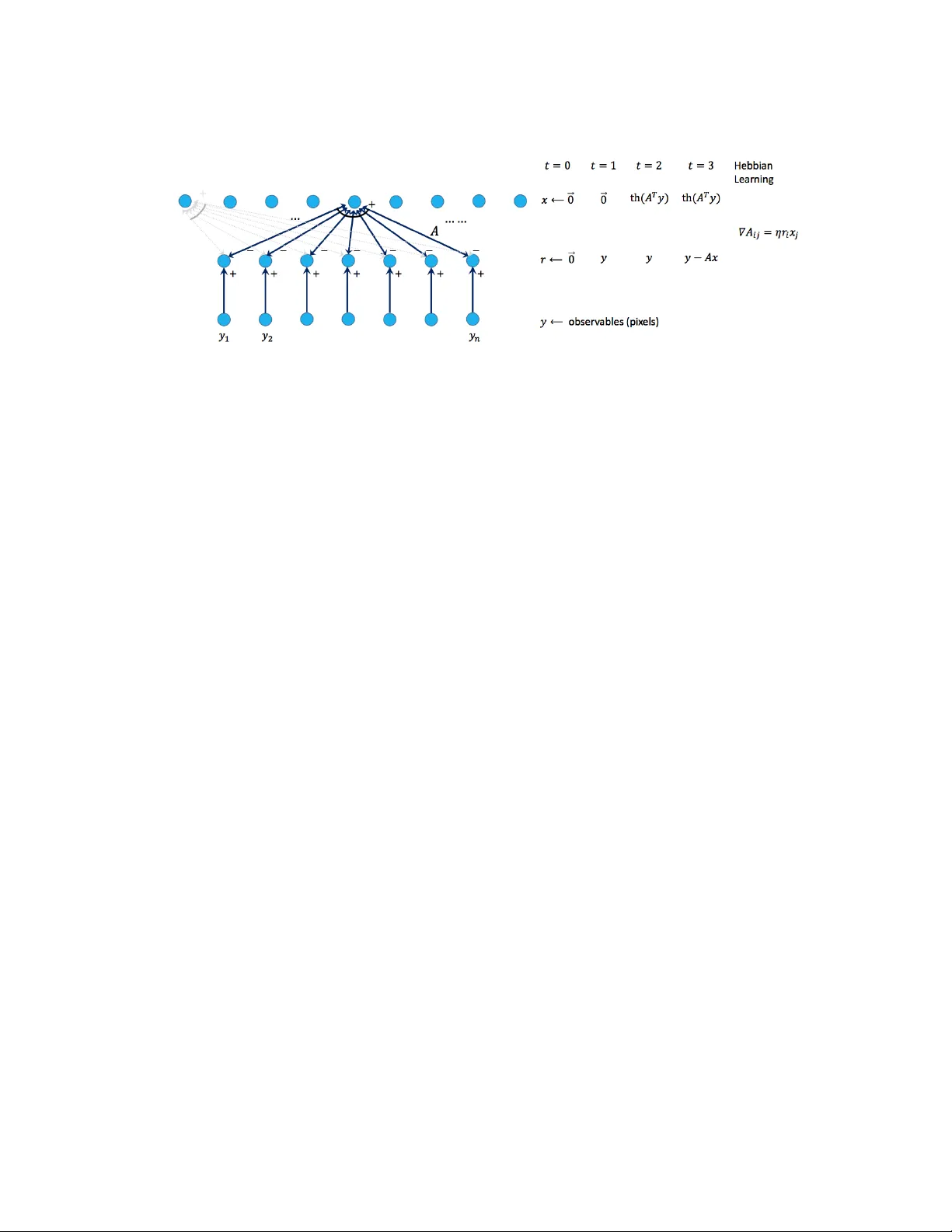
Simple, Eﬃcien t, and Neural Algorithms for Sparse Co ding Sanjeev Arora ∗ and Rong Ge † and T engyu Ma ‡ and Ankur Moitra § Abstract Sp arse c o ding is a basic task in many ﬁelds including signal pro cessing, neuroscience and mac hine learning where the goal is to learn a basis that enables a sparse representation of a given set of data, if one exists. Its standard formulation is as a non-conv ex optimization problem which is solved in practice by heuristics based on alternating minimization. Re- cen t w ork has resulted in several algorithms for sparse coding with pro v able guarantees, but somewhat surprisingly these are outp erformed b y the simple alternating minimization heuristics. Here we giv e a general framew ork for understanding alternating minimization whic h we leverage to analyze existing heuristics and to design new ones also with prov able guaran tees. Some of these algorithms seem implementable on simple neural architectures, whic h was the original motiv ation of Olshausen and Field ( 1997a ) in introducing sparse co ding. W e also giv e the ﬁrst eﬃcient algorithm for sparse co ding that works almost up to the information theoretic limit for sparse recov ery on incoherent dictionaries. All previous algorithms that approached or surpassed this limit run in time exponential in some natural parameter. Finally , our algorithms improv e up on the sample complexity of existing ap- proac hes. W e b eliev e that our analysis framew ork will hav e applications in other settings where simple iterative algorithms are used. 1. In tro duction Sp arse c o ding or dictionary le arning consists of learning to express (i.e., c o de ) a set of input v ectors, say image patches, as linear combinations of a smal l num b er of vectors chosen from a large dictionary . It is a basic task in man y ﬁelds. In signal pro cessing, a wide v ariety of signals turn out to b e sparse in an appropriately chosen basis (see references in Mallat ( 1998 )). In neuroscience, sparse represen tations are b eliev ed to improv e energy eﬃciency of the brain b y allo wing most neurons to b e inactive at an y given time. In mac hine learning, imp osing sparsity as a constraint on the represen tation is a useful wa y to av oid over-ﬁtting . Additionally , methods for sparse co ding can b e thought of as a to ol for fe atur e extr action and are the basis for a num b er of imp ortan t tasks in image pro cessing such as segmen tation, retriev al, de-noising and sup er-resolution (see references in Elad ( 2010 )), as § arora@cs.princeton.edu, Princeton Universit y , Computer Science Department and Center for Compu- tational Intractabilit y . This work w as supp orted in part by NSF gran ts CCF-0832797, CCF-1117309, CCF-1302518, DMS-1317308, Simons Inv estigator Award, and Simons Collab oration Grant. § rongge@microsoft.com, Microsoft Researc h, New England. § tengyu@cs.princeton.edu, Princeton Universit y , Computer Science Department and Center for Compu- tational Intractabilit y . This work w as supp orted in part by NSF gran ts CCF-0832797, CCF-1117309, CCF-1302518, DMS-1317308, Simons Inv estigator Award, and Simons Collab oration Grant. § moitra@mit.edu, Massach usetts Institute of T echnology , Department of Mathematics and CSAIL. This w ork w as supported in part by a grant from the MIT NEC Corp oration and a Go ogle Research Aw ard. w ell as a building blo c k for some deep learning architectures Ranzato et al. ( 2007 ). It is also a basic problem in linear algebra itself since it inv olv es ﬁnding a b etter basis. The notion w as introduced b y neuroscientists Olshausen and Field ( 1997a ) who formal- ized it as follows: Given a dataset y (1) , y (2) , . . . , y ( p ) ∈ < n , our goal is to ﬁnd a set of basis v ectors A 1 , A 2 , . . . , A m ∈ < n and sparse co eﬃcien t vectors x (1) , x (2) , . . . , x ( p ) ∈ < m that minimize the r e c onstruction err or p X i =1 k y ( i ) − A · x ( i ) k 2 2 + p X i =1 S ( x ( i ) ) (1) where A is the n × m c o ding matrix whose j th column is A j and S ( · ) is a nonlinear p enalt y function that is used to encourage sparsity . This function is nonconv ex b ecause b oth A and the x ( i ) ’s are unkno wn. Their pap er as w ell as subsequent w ork chooses m to b e larger than n (so-called over c omplete case) b ecause this allo ws greater ﬂexibilit y in adapting the represen tation to the data. W e remark that sparse co ding should not b e confused with the related — and usually easier — problem of ﬁnding the sparse representations of the y ( i ) ’s given the co ding matrix A , v ariously called c ompr esse d sensing or sp arse r e c overy Candes et al. ( 2006 ); Candes and T ao ( 2005 ). Olshausen and Field also gav e a local search/gradien t descent heuristic for trying to min- imize the noncon vex energy function ( 1 ). They gav e exp erimen tal evidence that it pro duces co ding matrices for image patches that resemble known features (such as Gab or ﬁlters) in V 1 p ortion of the visual cortex. A related pap er of the same authors Olshausen and Field ( 1997b ) (and also Lewic ki and Sejnowski ( 2000 )) places sparse co ding in a more familiar gener ative mo del setting whereby the data p oin ts y ( i ) ’s are assumed to b e probabilistically generated according to a model y ( i ) = A ∗ · x ∗ ( i ) + noise where x ∗ (1) , x ∗ (2) , . . . , x ∗ ( p ) are sam- ples from some appropriate distribution and A ∗ is an unknown co de. Then one can deﬁne the maximum lik eliho o d estimate, and this leads to a diﬀeren t and usually more complicated energy function — and asso ciated heuristics — compared to ( 1 ). Surprisingly , maximum likelihoo d-based approaches seem unnecessary in practice and lo cal search/gradien t descent on the energy function ( 1 ) with hard constraints works well, as do related algorithms such as MOD Aharon et al. ( 2006 ) and k -SVD Engan et al. ( 1999 ). In fact these metho ds are so eﬀective that sparse co ding is considered in practice to b e a solv ed problem, even though it has no p olynomial time algorithm p er se. Eﬃcien t Algorithms vs Neural Algorithms. Recen tly , there has b een rapid progress on designing p olynomial time algorithms for sparse co ding with prov able guarantees (the relev ant pap ers are discussed b elow). All of these adopt the generativ e mo del viewpoint sk etched ab o v e. But the surprising success of the simple descen t heuristics has remained largely unexplained. Empirically , these heuristics far out p erform — in running time, sample complexit y , and solution qualit y — the new algorithms, and this (startling) observ ation w as in fact the starting p oin t for the curren t work. Of course, the famous example of simplex vs el lipsoid for linear programming reminds us that it can b e muc h more challenging to analyze the b eha vior of an empirically successful algorithm than it is to to design a new p olynomial time algorithm from scratch! But for sparse coding the simple in tuitive heuristics are imp ortan t for another reason beyond just their algorithmic eﬃciency: they app ear to b e implementable in neural arc hitectures. 2 Simple, Efficient, and Neural Algorithms for Sp arse Coding (Roughly sp eaking, this means that the algorithm stores the co de matrix A as synapse w eights in a neural net work and up dates the entries using diﬀerences in p oten tials of the synapse’s endpoints.) Since neural computation — and also deep learning — ha ve prov en to b e diﬃcult to analyze in general, analyzing sparse coding thoroughly seems to b e a natural ﬁrst step for theory . Our algorithm is a close relativ e of the Olshausen-Field algorithm and th us inherits its neural implemen tability; see App endix E for further discussion. Here w e presen t a rigorous analysis of the simple energy minimization heuristic, and as a side b eneﬁt this yields b ounds on running time and sample complexity for sparse co ding that are b etter (in some cases, dramatically so) than the algorithms in recent pap ers. This adds to the recen t literature on analyzing alternating minimization Jain et al. ( 2013 ); Hardt ( 2013 ); Netrapalli et al. ( 2013 , 2014 ) but these work in a setting where there is a conv ex program that is kno wn to work to o, and in our setting, the only known con vex program runs in time exp onen tial in a natural parameter Barak et al. ( 2014 ). 1.1. Recen t W ork A common thread in recent w ork on sparse co ding is to assume a generative mo del; the precise details v ary , but each has the property that given enough samples the solution is essen tially unique. Spielman et al. ( 2012 ) gav e an algorithm that succeeds when A ∗ has full column rank (in particular m ≤ n ) whic h w orks up to sparsit y roughly √ n . How ev er this algorithm is not applicable in the more prev alent o v ercomplete setting. Arora et al. ( 2014 ) and Agarw al et al. ( 2013 , 2014 ) indep enden tly gav e algorithms in the o vercomplete case assuming that A ∗ is µ -incoherent (whic h we deﬁne in the next section). The former gav e an algorithm that works up to sparsit y n 1 / 2 − γ /µ for any γ > 0 but the running time is n Θ(1 /γ ) ; Agarw al et al. ( 2013 , 2014 ) ga ve an algorithm that w orks up to sparsity either n 1 / 4 /µ or n 1 / 6 /µ dep ending on the particular assumptions on the mo del. These w orks also analyze alternating minimization but assume that it starts from an estimate A that is column-wise 1 / p oly( n )-close to A ∗ , in which case the ob jective function is essen tially conv ex. Barak et al. ( 2014 ) gav e a new approac h based on the sum-of-squares hierarc hy that w orks for sparsit y up to n 1 − γ for any γ > 0. But in order to output an estimate that is column-wise  -close to A ∗ the running time of the algorithm is n 1 / O (1) . In most applications, one needs to set (say)  = 1 /k in order to get a useful estimate. Ho w ever in this case their algorithm runs in exp onen tial time. The sample complexit y of the ab o ve algorithms is also rather large, and is at least Ω( m 2 ) if not muc h larger. Here w e will giv e simple and more eﬃcient algorithms based on alternating minimization whose column-wise error decreases geometrically , and that work for sparsit y up to n 1 / 2 /µ log n . W e remark that ev en empirically , alternating minimization do es not appear to w ork muc h b ey ond this b ound. 1.2. Mo del, Notation and Results W e will work with the follo wing family of generative mo dels (similar to those in earlier pap ers) 1 : 1. The casual reader should just think of x ∗ as b eing drawn from some distribution that has independent co ordinates. Even in this simpler setting —which has p olynomial time algorithms using Indep endent Comp onent Analysis —w e do not know of an y rigorous analysis of heuristics lik e Olshausen-Field. The 3 Our Mo del Each sample is generated as y = A ∗ x ∗ + noise where A ∗ is a ground truth dictionary and x ∗ is dra wn from an unkno wn distribution D where (1) the supp ort S = supp( x ∗ ) is of size at most k , Pr [ i ∈ S ] = Θ( k /m ) and Pr [ i, j ∈ S ] = Θ( k 2 /m 2 ) (2) the distribution is normalized so that E [ x ∗ i | x ∗ j 6 = 0] = 0; E [ x ∗ i 2 | x ∗ i 6 = 0] = 1 and when x ∗ i 6 = 0, | x ∗ i | ≥ C for some constant C ≤ 1 and (3) the non-zero entries are pairwise indep endent and subgaussian, conditioned on the supp ort. (4) The noise is Gaussian and indep enden t across co ordinates. Suc h models are natural since the original motiv ation behind sparse co ding was to discov er a co de whose representations hav e the prop ert y that the co ordinates are almost independent. W e can relax most of the requirements ab o ve, at the exp ense of further restricting the sparsit y , but will not detail such tradeoﬀs. The rest of the pap er ignores the iid noise: it has little eﬀect on our basic steps lik e computing inner pro ducts of samples or taking singular vectors, and easily tolerated so long as it stays smaller than the “signal.” W e assume A ∗ is an incoherent dictionary , since these are widespread in signal processing Elad ( 2010 ) and statistics Donoho and Huo ( 1999 ), and include v arious families of wa v elets, Gab or ﬁlters as w ell as randomly generated dictionaries. Deﬁnition 1 An n × m matrix A whose c olumns ar e unit ve ctors is µ -inc oher ent if for al l i 6 = j we have h A i , A j i ≤ µ/ √ n. W e also require that k A ∗ k = O ( p m/n ). Ho wev er this can b e relaxed within polylogarithmic factors by tightening the bound on the sparsit y b y the same factor. Throughout this pap er w e will sa y that A s is ( δ , κ )-near to A ∗ if after a p erm utation and sign ﬂips its columns are within distance δ and we ha v e k A s − A ∗ k ≤ κ k A ∗ k . See also Deﬁnition 8 . W e will use this notion to measure the progress of our algorithms. Moreov er we will use g ( n ) = O ∗ ( f ( n )) to signify that g ( n ) is upp er b ounded by C f ( n ) for some small enough constan t C . Finally , throughout this pap er w e will assume that k ≤ O ∗ ( √ n/µ log n ) and m = O ( n ). Again, m can b e allow ed to b e higher by lo wering the sparsity . We assume al l these c onditions in our main the or ems. Main Theorems In Section 2 we give a general framework for analyzing alternating minimization. Instead of thinking of the algorithm as trying to minimize a kno wn non- con vex function, w e view it as trying to minimize an unknown con vex function. V arious up date rules are shown to provide go o d approximations to the gradient of the unknown function. See Lemma 11 , Lemma 28 and Lemma 33 for examples. W e then leverage our framew ork to analyze existing heuristics and to design new ones also with prov able guaran tees. In Section 3 , w e prov e: earlier papers were only in terested in p olynomial-time algorithms, so did not wish to assume indep en- dence. 4 Simple, Efficient, and Neural Algorithms for Sp arse Coding Theorem 2 Ther e is a neurally plausible algorithm which when initialize d with an esti- mate A 0 that is ( δ , 2) -ne ar to A ∗ for δ = O ∗ (1 / log n ) , c onver ges at a ge ometric r ate to A ∗ until the c olumn-wise err or is O ( p k /n ) . F urthermor e the running time is O ( mnp ) and the sample c omplexity is p = e O ( mk ) for e ach step. Additionally we giv e a neural architecture implementing our algorithm in App endix E . T o the b est of our kno wledge, this is the ﬁrst neurally plausible algorithm for sparse co ding with pro v able conv ergence. Ha ving set up our general framew ork and analysis technique w e can use it on other v ariants of alternating minimization. Section 3.1.2 gives a new up date rule whose bias (i.e., error) is negligible: Theorem 3 Ther e is an algorithm which when initialize d with an estimate A 0 that is ( δ, 2) - ne ar to A ∗ for δ = O ∗ (1 / log n ) , c onver ges at a ge ometric r ate to A ∗ until the c olumn-wise err or is O ( n − ω (1) ) . F urthermor e e ach step runs in time O ( mnp ) and the sample c omplexity p is p olynomial. This algorithm is based on a mo diﬁcation where we carefully pro ject out components along the column currently b eing updated. W e complement the ab o v e theorems by revisiting the Olshausen-Field rule and analyzing a v ariant of it in Section 3.1.1 (Theorem 12 ). How ever its analysis is more complex because we need to b ound some quadratic error terms. It uses con vex programming. What remains is to give a method to initialize these iterative algorithms. W e give a new approac h based on pair-wise rew eighting and w e pro ve that it returns an estimate A 0 that is ( δ, 2)-near to A ∗ for δ = O ∗ (1 / log n ) with high probabilit y . As an additional b eneﬁt, this algorithm can b e used ev en in settings where m is not kno wn and this could help solv e another problem in practice — that of mo del sele ction . In Section 5 w e prov e: Theorem 4 Ther e is an algorithm which r eturns an estimate A 0 that is ( δ, 2) -ne ar to A ∗ for δ = O ∗ (1 / log n ) . F urthermor e the running time is e O ( mn 2 p ) and the sample c omplexity p = e O ( mk ) . This algorithm also admits a neural implementation, which is sketc hed in App endix E . The pro of curren tly requires a pro jection step that increases the run time though we suspect it is not needed. W e remark that these algorithms w ork up to sparsit y O ∗ ( √ n/µ log n ) whic h is within a logarithmic factor of the information theoretic threshold for sparse recov ery on incoherent dictionaries Donoho and Huo ( 1999 ); Grib on v al and Nielsen ( 2003 ). All previous known algorithms that approac h Arora et al. ( 2014 ) or surpass this sparsity Barak et al. ( 2014 ) run in time exp onen tial in some natural parameter. Moreo ver, our algorithms are simple to describ e and implemen t, and inv olve only basic op erations. W e believe that our framework will hav e applications beyond sparse co ding, and could be used to sho w that simple, iterativ e algorithms can b e p o w erful in other contexts as well by suggesting new w ays to analyze them. 5 Algorithm 1 Generic Alternating Minimization Approach Initialize A 0 Rep eat for s = 0 , 1 , ..., T Deco de: Find a sparse solution to A s x ( i ) = y ( i ) for i = 1 , 2 , ..., p Set X s suc h that its columns are x ( i ) for i = 1 , 2 , ..., p Up date: A s +1 = A s − η g s where g s is the gradient of E ( A s , X s ) with resp ect to A s 2. Our F ramew ork, and an Overview Here we describ e our framework for analyzing alternating minimization. The generic sc heme w e will b e in terested in is given in Algorithm 1 and it alternates b et ween up dating the estimates A and X . It is a heuristic for minimizing the non-conv ex function in ( 1 ) where the p enalty function is a hard constraint. The crucial step is if we ﬁx X and compute the gradien t of ( 1 ) with resp ect to A , w e get: ∇ A E ( A, X ) = p X i =1 − 2( y ( i ) − Ax ( i ) )( x ( i ) ) T . W e then take a step in the opp osite direction to up date A . Here and throughout the pap er η is the learning rate, and needs to b e set appropriately . The c hallenge in analyzing this general algorithm is to identify a suitable “measure of progress”— called a Lyapuno v function in dynamical systems and con trol theory — and show that it impro v es at each step (with high probabilit y o ver the samples). W e will measure the progress of our algorithms b y the maximum column-wise diﬀerence b et w een A and A ∗ . In the next subsection, we identify suﬃcient conditions that guarantee progress. They are inspired by proofs in conv ex optimization. W e view Algorithm 1 as trying to minimize an unknown con vex function, sp eciﬁcally f ( A ) = E ( A, X ∗ ), which is strictly conv ex and hence has a unique optimum that can b e reached via gradien t descent. This function is unkno wn since the algorithm do es not know X ∗ . The analysis will show that the direction of mo vemen t is correlated with A ∗ − A s , which in turn is the gradient of the ab o ve func- tion. An indep endent pap er of Balakrishnan et al. ( 2014 ) prop oses a similar framew ork for analysing EM algorithms for hidden v ariable mo dels. The diﬀerence is that their condition is really ab out the geometry of the ob jective function, though ours is ab out the prop ert y of the direction of mo vemen t. Therefore we hav e the ﬂexibility to choose diﬀerent deco ding pro cedures. This ﬂexibilit y allows us to ha ve a closed form of X s and obtain a useful func- tional form of g s . The setup is reminiscen t of sto chastic gr adient desc ent , whic h mo ves in a direction whose exp ectation is the gradient of a known conv ex function. By contrast, here the function f () is unknown, and furthermore the exp ectation of g s is not the true gradient and has bias . Due to the bias, we will only b e able to pro ve that our algorithms reac h an appro ximate optimum up to some error whose magnitude is determined b y the bias. W e can mak e the bias negligible using more complicated algorithms. 6 Simple, Efficient, and Neural Algorithms for Sp arse Coding Appro ximate Gradient Descen t Consider a general iterativ e algorithm that is trying to get to a desired solution z ∗ (in our case z ∗ = A ∗ i for some i ). At step s it starts with a guess z s , computes some direction g s , and up dates its estimate as: z s +1 = z s − η g s . The natural progress measure is k z ∗ − z s k 2 , and b elo w we will identify a suﬃcien t condition for it to decrease in each step: Deﬁnition 5 A ve ctor g s is ( α, β ,  s )-correlated with z ∗ if h g s , z s − z ∗ i ≥ α k z s − z ∗ k 2 + β k g s k 2 −  s . R emark: The traditional analysis of conv ex optimization corresp onds to the setting where z ∗ is the global optim um of some con vex function f , and  s = 0. Sp eciﬁcally , if f ( · ) is 2 α -strongly conv ex and 1 / (2 β )-smooth, then g s = ∇ f ( z s ) ( α , β , 0)-correlated with z ∗ . Also w e will refer to  s as the bias. Theorem 6 Supp ose g s satisﬁes Deﬁnition 5 for s = 1 , 2 , . . . , T , and η satisﬁes 0 < η ≤ 2 β and  = max T s =1  s . Then for any s = 1 , . . . , T , k z s +1 − z ∗ k 2 ≤ (1 − 2 α η ) k z s − z ∗ k 2 + 2 η  s In p articular, the up date rule ab ove c onver ges to z ∗ ge ometric al ly with systematic err or /α in the sense that k z s − z ∗ k 2 ≤ (1 − 2 α η ) s k z 0 − z ∗ k 2 + /α . F urthermor e, if  s < α 2 k z s − z ∗ k 2 for s = 1 , . . . , T , then k z s − z ∗ k 2 ≤ (1 − α η ) s k z 0 − z ∗ k 2 . The pro of closely follo ws existing pro ofs in conv ex optimization: Pro of: [Proof of Theorem 6 ] W e expand the error as k z s +1 − z ∗ k 2 = k z s − z ∗ k 2 − 2 η g s T ( z s − z ∗ ) + η 2 k g s k 2 = k z s − z ∗ k 2 − η  2 g s T ( z s − z ∗ ) − η k g s k 2  ≤ k z s − z ∗ k 2 − η  2 α k z s − z ∗ k 2 + (2 β − η ) k g s k 2 − 2  s  (Deﬁnition 5 and η ≤ 2 β ) ≤ k z s − z ∗ k 2 − η  2 α k z s − z ∗ k 2 − 2  s  ≤ (1 − 2 α η ) k z s − z ∗ k 2 + 2 η  s Then solving this recurrence we ha ve k z s +1 − z ∗ k 2 ≤ (1 − 2 αη ) s +1 R 2 +  α where R = k z 0 − z ∗ k . And furthermore if  s < α 2 k z s − z ∗ k 2 w e hav e instead k z s +1 − z ∗ k 2 ≤ (1 − 2 α η ) k z s − z k 2 + α η k z s − z k 2 = (1 − αη ) k z s − z k 2 and this yields the second part of the theorem to o.  In fact, we can extend the analysis ab o ve to obtain identical results for the case of constrained optimization. Supp ose we are interested in optimizing a conv ex function f ( z ) 7 o ver a con vex set B . The standard approac h is to tak e a step in the direction of the gradien t (or g s in our case) and then pro ject in to B after eac h iteration, namely , replace z s +1 b y Pro j B z s +1 whic h is the closest p oint in B to z s +1 in Euclidean distance. It is well-kno wn that if z ∗ ∈ B , then k Pro j B z − z ∗ k ≤ k z − z ∗ k . Therefore we obtain the following as an immediate corollary to the ab o ve analysis: Corollary 7 Supp ose g s satisﬁes Deﬁnition 5 for s = 1 , 2 , . . . , T and set 0 < η ≤ 2 β and  = max T s =1  s . F urther supp ose that z ∗ lies in a c onvex set B . Then the up date rule z s +1 = Pr oj B ( z s − η g s ) satisﬁes that for any s = 1 , . . . , T , k z s − z ∗ k 2 ≤ (1 − 2 α η ) s k z 0 − z ∗ k 2 + /α In p articular, z s c onver ges to z ∗ ge ometric al ly with systematic err or /α . A dditional ly if  s < α 2 k z s − z ∗ k 2 for s = 1 , . . . , T , then k z s − z ∗ k 2 ≤ (1 − α η ) s k z 0 − z ∗ k 2 What remains is to derive a functional form for v arious up date rules and show that these rules mo ve in a direction g s that appro ximately p oin ts in the direction of the desired solution z ∗ (under the assumption that our data is generated from a stochastic model that meets certain conditions). An Ov erview of Applying Our F ramework Our framew ork clariﬁes that an y improv ement step meeting Deﬁnition 5 will also conv erge to an appro ximate optimum, which enables us to engineer other up date rules that turn out to b e easier to analyze. Indeed we ﬁrst analyze a simpler up date rule with g s = E [( y − A s x )sgn( x T )] in Section 3 . Here sgn( · ) is the co ordinate-wise sign function. W e then return to the Olshausen-Field up date rule and analyze a v ariant of it in Section 3.1.1 using approximate pro jected gradient descent. Finally , we design a new up date rule in Section 3.1.2 where w e carefully pro ject out comp onen ts along the column currently b eing up dated. This has the eﬀect of replacing one error term with another and results in an up date rule with negligible bias. The main steps in showing that these up date rules ﬁt in to our framew ork are giv en in Lemma 11 , Lemma 28 and Lemma 33 . Ho w should the algorithm up date X ? The usual approach is to solve a sparse reco very problem with resp ect to the curren t co de matrix A . How ev er man y of the standard basis pursuit algorithms (such as solving a linear program with an ` 1 p enalt y) are diﬃcult to analyze when there is error in the co de itself. This is in part because the solution do es not ha ve a closed form in terms of the co de matrix. Instead w e take a muc h simpler approac h to solving the sparse reco very problem whic h uses matrix-v ector m ultiplication follow ed by thresholding: In particular, we set x = threshold C / 2 (( A s ) T y ), where threshold C / 2 ( · ) keeps only the co ordinates whose magnitude is at least C / 2 and zeros out the rest. Recall that the non-zero co ordinates in x ∗ ha ve magnitude at least C . This deco ding rule reco v ers the signs and support of x correctly provided that A is column-wise δ -close to A ∗ for δ = O ∗ (1 / log n ). See Lemma 10 . The rest of the analysis can b e describ ed as follows: If the signs and supp ort of x are reco vered correctly , then alternating minimization mak es progress in each step. In fact this 8 Simple, Efficient, and Neural Algorithms for Sp arse Coding holds each for m uch larger v alues of k than we consider; as high as n/ (log n ) O (1) . (How ev er, the explicit deco ding rule fails for k > √ n/µ log n .) Thus it only remains to prop erly initialize A 0 so that it is close enough to A ∗ to let the ab o v e deco ding rule succeed. In Section 5 we give a new initialization pro cedure based on pair-wise reweigh ting that we pro ve works with high probability . This section may b e of indep enden t in terest, since this algorithm can b e used ev en in settings where m is not kno wn and could help solve another problem in practice — that of mo del sele ction . See Lemma 20 . 3. A Neurally Plausible Algorithm with Prov able Guaran tees Here we will design and analyze a neurally plausible algorithm for sparse co ding whic h is giv en in Algorithm 2 , and we giv e a neural architecture implemen ting our algorithm in App endix E . The fact that such a simple algorithm pro v ably works sheds new light on ho w sparse co ding might b e accomplished in nature. Here and throughout this pap er w e will w ork with the follo wing measure of closeness: Deﬁnition 8 A is δ -close to A ∗ if ther e is a p ermutation π : [ m ] → [ m ] and a choic e of signs σ : [ m ] → {± 1 } such that k σ ( i ) A π ( i ) − A ∗ i k ≤ δ for al l i We say A is ( δ, κ )-near to A ∗ if in addition k A − A ∗ k ≤ κ k A ∗ k to o. This is a natural measure to use, since we can only hop e to learn the columns of A ∗ up to relab eling and sign-ﬂips. In our analysis, w e will assume throughout that π ( · ) is the iden tity p erm utation and σ ( · ) ≡ +1 b ecause our family of generativ e mo dels is inv ariant under this relab eling and it will simplify our notation. Let sgn( · ) denote the coordinate-wise sign function and recall that η is the learning rate, whic h we will so on set. Also we ﬁx b oth δ, δ 0 = O ∗ (1 / log n ). W e will also assume that in eac h iteration, our algorithm is given a fresh set of p samples. Our main theorem is: Theorem 9 Supp ose that A 0 is (2 δ, 2) -ne ar to A ∗ and that η = Θ( m/k ) . Then if e ach up date step in A lgorithm 2 uses p = e Ω( mk ) fr esh samples, we have E [ k A s i − A ∗ i k 2 ] ≤ (1 − τ ) s k A 0 i − A ∗ i k 2 + O ( k /n ) for some 0 < τ < 1 / 2 and for any s = 1 , 2 , ..., T . In p articular it c onver ges to A ∗ ge ometri- c al ly, until the c olumn-wise err or is O ( p k /n ) . Our strategy is to pro v e that b g s is ( α , β ,  )-correlated (see Deﬁnition 5 ) with the desired solution A ∗ , and then to prov e that k A k nev er gets to o large. W e will ﬁrst prov e that if A is somewhat close to A ∗ then the estimate x for the representation almost alw ays has the correct supp ort. Here and elsewhere in the pap er, we use “very high probability” to mean that an even t happ ens with probabilit y at least 1 − 1 /n ω (1) . Lemma 10 Supp ose that A s is δ -close to A ∗ . Then with very high pr ob ability over the choic e of the r andom sample y = A ∗ x ∗ : sgn(threshold C / 2 (( A s ) T y )) = sgn( x ∗ ) 9 Algorithm 2 Neurally Plausible Up date Rule Initialize A 0 that is ( δ 0 , 2)-near to A ∗ Rep eat for s = 0 , 1 , ..., T Deco de: x ( i ) = threshold C / 2 (( A s ) T y ( i ) ) for i = 1 , 2 , ..., p Up date: A s +1 = A s − η b g s where b g s = 1 p · p X i =1 ( y ( i ) − A s x ( i ) )sgn( x ( i ) ) T W e pro ve a more general version of this lemma (Lemma 23 ) in Appendix A ; it is an ingredien t in analyzing all of the update rules w e consider in this pap er. How ever this is just one step on the wa y to wards pro ving that b g s is correlated with the true solution. The next step in our pro of is to use the prop erties of the generativ e mo del to deriv e a new form ula for b g s that is more amenable to analysis. W e deﬁne g s to b e the exp ectation of b g s g s := E [ b g s ] = E [( y − A s x )sgn( x ) T ] (2) where x := threshold C / 2 (( A s ) T y ) is the deco ding of y . Let q i = Pr [ x ∗ i 6 = 0] and q i,j = Pr [ x ∗ i x ∗ j 6 = 0], and deﬁne p i = E [ x ∗ i sgn( x ∗ i ) | x ∗ i 6 = 0]. Here and in the rest of the pap er, we will let γ denote an y vector whose norm is negligible (i.e. smaller than 1 /n C for any large constant C > 1). This will simplify our calculations. Also let A ∗ − i denote the matrix obtained from deleting the i th column of A ∗ . The follo wing lemma is the main step in our analysis. Lemma 11 Supp ose that A s is (2 δ, 2) -ne ar to A ∗ . Then the up date step in Algorithm 2 takes the form E [ A s +1 i ] = A s i − η g s i wher e g s i = p i q i ( λ s i A s i − A ∗ i +  s i ± γ ) , and λ s i = h A s i , A ∗ i i and  s i =  A s − i diag ( q i,j )  A s − i  T  A ∗ i /q i Mor e over the norm of  s i c an b e b ounde d as k  s i k ≤ O ( k /n ) . Note that p i q i is a scaling constant and λ i ≈ 1; hence from the ab ov e form ula we should exp ect that g s i is w ell-correlated with A s i − A ∗ i . Pro of: Since A s is (2 δ, 2)-near to A ∗ , A s is 2 δ -close to A ∗ . W e can now in vok e Lemma 10 and conclude that with high probabilit y , sgn( x ∗ ) = sgn( x ). Let F x ∗ b e the even t that sgn( x ∗ ) = sgn( x ), and let 1 F x ∗ b e the indicator function of this even t. T o av oid the ov erwhelming n umber of app earances of the sup erscripts, let B = A s throughout this pro of. Then w e can write g s i = E [( y − B x )sgn( x i )]. Using the fact that 1 F x ∗ + 1 ¯ F x ∗ = 1 and that F x ∗ happ ens with v ery high probability: g s i = E [( y − B x )sgn( x i ) 1 F x ∗ ] + E [( y − B x )sgn( x i ) 1 F x ∗ ] = E [( y − B x )sgn( x i ) 1 F x ∗ ] ± γ (3) The k ey is that this allo ws us to essen tially replace sgn( x ) with sgn( x ∗ ). Moreov er, let S = supp( x ∗ ). Note that when F x ∗ happ ens S is also the supp ort of x . Recall that 10 Simple, Efficient, and Neural Algorithms for Sp arse Coding according to the deco ding rule (where we ha v e replaced A s b y B for notational simplicit y) x = threshold C / 2 ( B T y ). Therefore, x S = ( B T y ) S = B T S y = B T S A ∗ x ∗ . Using the fact that the supp ort of x is S again, we ha ve B x = B T S B S A ∗ x ∗ . Plugging it into equation ( 3 ): g s i = E [( y − B x )sgn( x i ) 1 F x ∗ ] ± γ = E [( I − B S B T S ) A ∗ x ∗ · sgn( x ∗ i ) 1 F x ∗ ] ± γ = E [( I − B S B T S ) A ∗ x ∗ · sgn( x ∗ i )] − E [( I − B S B T S ) A ∗ x ∗ · sgn( x i ) 1 ¯ F x ∗ ] ± γ = E [( I − B S B T S ) A ∗ x · sgn( x ∗ i )] ± γ where again we hav e used the fact that F x ∗ happ ens with v ery high probabilit y . No w we rewrite the expectation ab ov e using sub conditioning where we ﬁrst choose the supp ort S of x ∗ , and then we choose the nonzero v alues x ∗ S . E [( I − B S B T S ) A ∗ x ∗ · sgn( x ∗ i )] = E S h E x ∗ S [( I − B S B T S ) A ∗ x ∗ · sgn( x ∗ i ) | S ] i = E [ p i ( I − B S B T S ) A ∗ i ] where w e use the fact that E [ x ∗ i · sgn( x ∗ i ) | S ] = p i . Let R = S − { i } . Using the fact that B S B T S = B i B T i + B R B T R , w e can split the quantit y ab o v e into t w o parts, g s i = p i E [( I − B i B T i ) A ∗ i + p i E [ B R B T R ] A ∗ i = p i q i  I − B i B T i  A ∗ i + p i  B − i diag( q i,j ) B T − i  A ∗ i ± γ . where diag( q i,j ) is a m × m diagonal matrix whose ( j, j )-th entry is equal to q i,j , and B − i is the matrix obtained by zeroing out the i th column of B . Here w e used the fact that Pr [ i ∈ S ] = q i and Pr [ i, j ∈ S ] = q ij . No w w e set B = A s , and rearranging the terms, w e hav e g s i = p i q i ( h A s i , A ∗ i i A s i − A ∗ i +  s i ± γ ) where  s i =  A s − i diag( q i,j )  A s − i  T  A ∗ i /q i , whic h can b e bounded as follo ws k  s i k ≤ k A s − i k 2 max j 6 = i q i,j /q i ≤ O ( k /m ) k A s k 2 = O ( k/n ) where the last step used the fact that max i 6 = j q i,j min q i ≤ O ( k/m ), which is an assumption of our generativ e mo del.  W e will b e able to reuse muc h of this analysis in Lemma 28 and Lemma 33 b ecause we ha ve deriv ed to for a general deco ding matrix B . In Section 4 w e complete the analysis of Algorithm 2 in the inﬁnite sample setting. In particular, in Section 4.1 , we pro ve that if A s is (2 δ, 2)-near to A ∗ then g s i is indeed ( α, β ,  )-correlated with A i (Lemma 16 ). Finally we prov e that if A s is (2 δ, 2)-near to A ∗ then k A s +1 − A ∗ k ≤ 2 k A ∗ k (Lemma 17 ). These lemmas together with Theorem 6 imply Theorem 14 , the simpliﬁed version of Theorem 9 where the num b er of samples p is assumed to be inﬁnite (i.e. w e hav e access to the true exp ectation g s ). In Appendix D w e prov e the sample complexit y b ounds we need and this completes the pro of of Theorem 9 . 3.1. F urther Applications Here we apply our framew ork to design and analyze further v ariants of alternating mini- mization. 11 3.1.1. Revisiting Olshausen-Field In this subsection w e analyze a v arian t of the Olshausen-Field up date rule. How ev er there are quadratic error terms that arise in the expressions w e deriv e for g s and bounding them is more c hallenging. W e will also need to make (slightly) stronger assumptions on the distributional mo del that for distinct i 1 , i 2 , i 3 w e hav e q i 1 ,i 2 ,i 3 = O ( k 3 /m 3 ) where q i 1 ,i 2 ,i 3 = Pr [ i 1 , i 2 , i 3 ∈ S ]. Theorem 12 Supp ose that A 0 is (2 δ, 2) -ne ar to A ∗ and that η = Θ( m/k ) . Ther e is a variant of Olshausen-Field (given in Algorithm 4 in App endix B.1 ) for which at e ach step s we have k A s − A ∗ k 2 F ≤ (1 − τ ) s k A 0 − A ∗ k 2 F + O ( mk 2 /n 2 ) for some 0 < τ < 1 / 2 and for any s = 1 , 2 , ..., T . In p articular it c onver ges to A ∗ ge ometri- c al ly until the err or in F r ob enius norm is O ( √ mk /n ) . W e defer the pro of of the main theorem to App endix B.1 . Curren tly it uses a pro jection step (using conv ex programming) that may not b e needed but the pro of requires it. 3.1.2. Removing the Systemic Err or In this subsection, w e design and analyze a new up date rule that conv erges geometrically un til the column-wise error is n − ω (1) . The basic idea is to engineer a new deco ding matrix that pro jects out the comp onen ts along the column currently b eing up dated. This has the eﬀect of replacing a certain error term in Lemma 11 with another term that go es to zero as A gets closer to A ∗ (the earlier rules we hav e analyzed do not hav e this prop ert y). W e will use B ( s,i ) to denote the decoding matrix used when up dating the i th column in the s th step. Then w e set B ( s,i ) i = A i and B ( s,i ) j = Pro j A ⊥ i A j for j 6 = i . Note that B ( s,i ) − i (i.e. B ( s,i ) with the i th column remov ed) is no w orthogonal to A i . W e will rely on this fact when w e b ound the error. W e defer the pro of of the main theorem to App endix B.2 . Theorem 13 Supp ose that A 0 is (2 δ, 2) -ne ar to A ∗ and that η = Θ( m/k ) . Ther e is an algorithm (given in Algorithm 5 given in App endix B.2 ) for which at e ach step s , we have k A s i − A ∗ i k 2 ≤ (1 − τ ) s k A 0 i − A ∗ i k 2 + n − ω (1) for some 0 < τ < 1 / 2 and for any s = 1 , 2 , ..., T . In p articular it c onver ges to A ∗ ge ometri- c al ly until the c olumn-wise err or is n − ω (1) . 4. Analysis of the Neural Algorithm In Lemma 11 we ga ve a new (and more useful) expression that describ es the up date direction under the assumptions of our generative mo del. Here w e will make crucial use of Lemma 11 in order to prov e that g s i is ( α, β ,  )-correlated with A i (Lemma 15 ). Moreov er we use Lemma 11 again to show that k A s +1 − A ∗ k ≤ 2 k A ∗ k (Lemma 17 ). T ogether, these auxiliary lemmas imply that the column-wise error decreases in the next step and moreo ver the errors across columns are uncorrelated. 12 Simple, Efficient, and Neural Algorithms for Sp arse Coding W e assume that eac h iteration of Algorithm 2 tak es inﬁnite n umber of samples, and prov e the corresp onding simpliﬁed version of Theorem 9 . The pro of of this Theorem highlights the essen tial ideas of b ehind the proof of the Theorem 9 , which can be found at Appendix D . Theorem 14 Supp ose that A 0 is (2 δ, 2) -ne ar to A ∗ and that η = Θ( m/k ) . Then if e ach up date step in A lgorithm 2 uses inﬁnite numb er of samples at e ach iter ation, we have k A s i − A ∗ i k 2 ≤ (1 − τ ) s k A 0 i − A ∗ i k 2 + O ( k 2 /n 2 ) for some 0 < τ < 1 / 2 and for any s = 1 , 2 , ..., T . In p articular it c onver ges to A ∗ ge ometri- c al ly until the c olumn-wise err or is O ( k /n ) . The pro of is deferred to the end of this section. 4.1. Making Progress In Lemma 11 we sho wed that g s i = p i q i ( λ i A s i − A ∗ i +  s i + γ ) where λ i = h A i , A ∗ i i . Here we will prov e that g s i is ( α, β ,  )-correlated with A ∗ i . Recall that we ﬁxed δ = O ∗ (1 / log n ). The main in tuition is that g s i is mostly equal to p i q i ( A s i − A ∗ i ) with a small error term. Lemma 15 If a ve ctor g s i is e qual to 4 α ( A s i − A ∗ i ) + v wher e k v k ≤ α k A s i − A ∗ i k + ζ , then g s i is ( α, 1 / 100 α, ζ 2 /α ) -c orr elate d with A ∗ i , mor e sp e ciﬁc al ly, h g s i , A s i − A ∗ i i ≥ α k A s i − A ∗ i k 2 + 1 100 α k g i k 2 − ζ 2 /α. In particular, g s i is ( α, β ,  )-correlated with A ∗ i , where α = Ω( k /m ), β ≥ Ω( m/k ) and  = O ( k 3 /mn 2 ). W e can no w apply Theorem 6 and conclude that the column-wise error gets smaller in the next step: Corollary 16 If A s is (2 δ, 2) -ne ar to A ∗ and η ≤ min i ( p i q i (1 − δ )) = O ( m/k ) , then g s i = p i q i ( λ i A s i − A ∗ i +  s i + γ ) is (Ω( k /m ) , Ω( m/k ) , O ( k 3 /mn 2 )) -c orr elate d with A ∗ i , and further k A s +1 i − A ∗ i k 2 ≤ (1 − 2 α η ) k A s i − A ∗ i k 2 + O ( η k 2 /n 2 ) Pro of: [Proof of Lemma 15 ] Throughout this pro of s is ﬁxed and so we will omit the su- p erscript s to simplify notations. By the assumption, g i already has a comp onen t that is p oin ting to the correct direction A i − A ∗ i , we only need to show that the norm of the extra term v is small enough. First we can b ound the norm of g i b y triangle inequality: k g i k ≤ k 4 α ( A i − A ∗ i ) k + k v k ≤ 5 α k ( A i − A ∗ i ) k + ζ , therefore k g i k 2 ≤ 50 α 2 k ( A i − A ∗ i ) k 2 + 2 ζ 2 . Also, we can b ound the inner-pro duct b et ween g i and A i − A ∗ i b y h g i , A i − A ∗ i i ≥ 4 α k A i − A ∗ i k 2 − k v kk A i − A ∗ i k . 13 Using these b ounds, we will show h g i , A i − A ∗ i i − α k A i − A ∗ i k 2 − 1 100 α k g i k 2 + ζ 2 /α ≥ 0. Indeed w e hav e h g i , A i − A ∗ i i − α k A i − A ∗ i k 2 − 1 100 α k g i k 2 + ζ 2 /α ≥ 4 α k A i − A ∗ i k 2 − k v kk A i − A ∗ i k − α k A i − A ∗ i k 2 − 1 100 α k g i k 2 + ζ 2 /α ≥ 3 α k A i − A ∗ i k 2 − ( α k A i − A ∗ i k + ζ ) k A i − A ∗ i k − 1 100 α (50 α 2 k ( A i − A ∗ i ) k 2 + 2 ζ 2 ) + ζ 2 /α ≥ α k A i − A ∗ i k 2 − ζ k A i − A ∗ i k + 1 4 ζ 2 /α = ( √ α k A i − A ∗ i k − ζ / 2 √ α ) 2 ≥ 0 . This completes the pro of of the lemma.  Pro of: [Proof of Corollary 16 ] W e use the form in Lemma 11 , g s i = p i q i ( λ i A s i − A ∗ i +  s i + γ ) where λ i = h A i , A ∗ i i . W e can write g s i = p i q i ( A s i − A ∗ i ) + p i q i ((1 − λ i ) A s i +  s i + γ ), so when applying Lemma 15 w e can use 4 α = p i q i = Θ( k /m ) and v = p i q i ((1 − λ i ) A s i +  s i + γ ). The norm of v can be b ounded in t wo terms, the ﬁrst term p i q i (1 − λ i ) A s i has norm p i q i (1 − λ i ) whic h is smaller than p i q i k A s i − A ∗ i k , and the second term has norm b ounded by ζ = O ( k 2 /mn ). By Lemma 15 we kno w the vector g i s is (Ω( k /m ) , Ω( m/k ) , O ( k 3 /mn 2 ))-correlated with A s . Then by Theorem 6 w e hav e the last part of the corollary .  4.2. Main taining Nearness Lemma 17 Supp ose that A s is (2 δ, 2) -ne ar to A ∗ . Then k A s +1 − A ∗ k ≤ 2 k A ∗ k in Algo- rithm 2 . Pro of: As in the pro of of the previous lemma, we will mak e crucial use of Lemma 11 . Substituting and rearranging terms we ha v e: A s +1 i − A ∗ i = A s i − A ∗ i − η g s i = (1 − η p i q i )( A s i − A ∗ i ) + η p i q i (1 − λ s i ) A s i − η p i  A s − i diag( q i,j )  A s − i  T  A ∗ i ± γ Our ﬁrst goal is to write this equation in a more conv enien t form. In particular let U and V be matrices suc h that U i = p i q i (1 − λ s i ) A s i and V i = p i  A s − i diag( q i,j )  A s − i  T  A ∗ i . Then w e can re-write the ab o ve equation as: A s +1 − A ∗ = ( A s − A ∗ )diag(1 − η p i q i ) + η U − η V ± γ where diag(1 − η p i q i ) is the m × m diagonal matrix whose en tries along the diagonal are 1 − η p i q i . W e will b ound the spectral norm of A s +1 − A b y b ounding the sp ectral norm of each of the matrices of right hand side. The ﬁrst tw o terms are straightforw ard to b ound: k ( A s − A ∗ )diag(1 − η p i q i ) k ≤ k A s − A ∗ k · (1 − η min i p i q i ) ≤ 2(1 − Ω( η k /m )) k A ∗ k 14 Simple, Efficient, and Neural Algorithms for Sp arse Coding where the last inequalit y uses the assumption that p i = Θ(1) and q i ≤ O ( k/m ), and the assumption that k A s − A ∗ k ≤ 2 k A ∗ k . F rom the deﬁnition of U it follows that U = A s diag( p i q i (1 − λ s i )), and therefore k U k ≤ δ max i p i q i k A s k = o ( k /m ) · k A ∗ k where we hav e used the fact that λ s i ≥ 1 − δ and δ = o (1), and k A s k ≤ k A s − A ∗ k + k A ∗ k = O ( k A ∗ k ). What remains is to bound the third term, and let us ﬁrst introduce an auxiliary matrix Q which w e deﬁne as follows: Q ii = 0 and Q i,j = q i,j h A s i , A ∗ i i for i 6 = j . It is easy to verify that the following claim: Claim 18 The i th c olumn of A s Q is e qual to  A s − i diag ( q i,j )  A s − i  T  A ∗ i Therefore we can write V = A s Q diag( p i ). W e will b ound the sp ectral norm of Q by b ounding its F rob en us norm instead. Then from the deﬁnition of A , we ha v e that: k Q k F ≤  max i 6 = j q ij  X i 6 = j q h A s i , A ∗ j i 2 = O ( k 2 /m 2 ) k A ∗ T A s k F Moreo ver since A ∗ T A s is an m × m matrix, its F rob enius norm can b e at most a √ m factor larger than its sp ectral norm. Hence we hav e k V k ≤  max i p i  k A s kk Q k ≤ O ( k 2 √ m/m 2 ) k A s k 2 k A ∗ k ≤ o ( k /m ) k A ∗ k where the last inequality uses the fact that k = O ( √ n/ log n ) and k A s k ≤ O ( k A ∗ k ). Therefore, putting the pieces together we ha ve: k A s +1 − A ∗ k ≤ k ( A s − A ∗ )diag(1 − η p i q i ) k + k η U k + k η V k ± γ ≤ 2(1 − Ω( η k/m )) k A k + o ( η k/m ) k A ∗ k + o ( η k /m ) k A ∗ k ± γ ≤ 2 k A ∗ k and this completes the pro of of the lemma.  4.3. Pro of of Theorem 14 W e pro ve b y induction on s . Our induction hypothesis is that the theorem is true at eac h step s and A s is (2 δ, 2)-near to A ∗ . The h yp othesis is trivially true for s = 0. Now assuming the inductive h yp othesis is true. Recall that Corollary 16 of Section 4.1 says that if A s is (2 δ, 2)-near to A ∗ , which is guaranteed b y the inductive hypothesis, b y then g s i is indeed (Ω( k /m ) , Ω( m/k ) , O ( k 3 /mn 2 ))-correlated with A ∗ i . In voking our framew ork of analysis (Theorem 6 ), we hav e that k A s +1 i − A ∗ i k 2 ≤ (1 − τ ) k A s i − A ∗ i k 2 + O ( k 2 /n 2 ) ≤ (1 − τ ) s +1 k A 0 i − A ∗ i k 2 + O ( k 2 /n 2 ) Therefore it also follows that A s +1 is 2 δ -close to A ∗ . Then we in vok e Lemma 17 to pro ve A s +1 has not to o large sp ectral norm k A s +1 − A ∗ k ≤ 2 k A ∗ k , which completes the induction. 15 Algorithm 3 P airwise Initialization Set L = ∅ While | L | < m choose samples u and v Set c M u,v = 1 p 2 P p 2 i =1 h y ( i ) , u ih y ( i ) , v i y ( i ) ( y ( i ) ) T Compute the top tw o singular v alues σ 1 , σ 2 and top singular vector z of c M u,v If σ 1 ≥ Ω( k /m ) and σ 2 < O ∗ ( k /m log m ) If z is not within distance 1 / log m of an y vector in L (even after sign ﬂip), add z to L Set e A such that its columns are z ∈ L and output A = Pro j B e A where B is the conv ex set deﬁned in Deﬁnition 30 5. Initialization There is a large gap b et w een theory and practice in terms of how to initialize alternating minimization. The usual approach is to set A randomly or to p opulate its columns with samples y ( i ) . These often work but we do not know ho w to analyse them. Here w e give a nov el metho d for initialization which we sho w succeeds with v ery high probability . Our algorithm works b y pairwise reweigh ting. Let u = A ∗ α and v = A ∗ α 0 b e t wo samples from our mo del whose supp orts are U and V resp ectively . The main idea is that if we reweigh t fresh samples y with a factor h y , u ih y , v i and compute c M u,v = 1 p 2 p 2 X i =1 h y ( i ) , u ih y ( i ) , v i y ( i ) ( y ( i ) ) T then the top singular vectors will corresp ond to columns A ∗ j where j ∈ U ∩ V . (This is reminiscen t of ideas in recen t pap ers on dictionary learning, but more sample eﬃcient.) Throughout this section w e will assume that the algorithm is given tw o sets of samples of size p 1 and p 2 resp ectiv ely . Let p = p 1 + p 2 . W e use the ﬁrst set of samples for the pairs u, v that are used in rew eighting and w e use the second set to compute c M u,v (that is, the same set of p 2 samples is used for each u, v throughout the execution of the algorithm). Our main theorem is: Theorem 19 Supp ose that Algorithm 3 is given p 1 = e Ω( m ) and p 2 = e Ω( mk ) fr esh samples and mor e over ( a ) A ∗ is µ -inc oher ent with µ = O ∗ ( √ n k log 3 n ) , ( b ) m = O ( n ) and ( c ) k A ∗ k ≤ O ( p m n ) . Then with high pr ob ability A is ( δ, 2) -ne ar to A ∗ wher e δ = O ∗ (1 / log n ) . W e will defer the pro of of this theorem to App endix C . The key idea is the following main lemma. W e will inv oke this lemma sev eral times in order to analyze Algorithm 3 to v erify whether or not the supp orts of u and v share a common elemen t, and again to sho w that if they do we can approximately recov er the corresp onding column of A ∗ from the top singular v ector of M u,v . 16 Simple, Efficient, and Neural Algorithms for Sp arse Coding Lemma 20 Supp ose u = A ∗ α and v = A ∗ α 0 ar e two r andom samples with supp orts U , V r esp e ctively. L et β = A ∗ T u and β 0 = A ∗ T v . L et y = A ∗ x ∗ b e r andom sample that is indep endent of u , v , then M u,v := E [ h u, y ih v , y i y y T ] = X i ∈ U ∩ V q i c i β i β 0 i A ∗ i A ∗ i T + E 1 + E 2 + E 3 , (4) wher e q i = Pr [ i ∈ S ] , c i = E [ x ∗ i 4 | i 6 = S ] , and the err or terms ar e: E 1 = P i 6∈ U ∩ V q i c i β i β 0 i A ∗ i A ∗ i T E 2 = P i,j ∈ [ m ] ,i 6 = j q i,j β i β 0 i A ∗ j A ∗ j T E 3 = P i,j ∈ [ m ] ,i 6 = j q i,j ( β i A ∗ i β 0 j A ∗ j T + β 0 i A ∗ i β j A ∗ j T ) . Mor e over the err or terms E 1 + E 2 + E 3 has sp e ctr al norm b ounde d by O ∗ ( k /m log n ) , | β i | ≥ Ω(1) for al l i ∈ supp( α ) and | β 0 i | ≥ Ω(1) for al l i ∈ supp( α 0 ) . Pro of: [Proof of Lemma 20 ] W e will pro ve this lemma in three parts. First we compute the exp ectation and sho w it has the desired form. Recall that y = A ∗ x ∗ , and so: M u,v = E S h E x ∗ S [ h u, A ∗ S x ∗ S ih v , A ∗ S x ∗ S i A ∗ S x ∗ S x ∗ S T A ∗ S T | S ] i = E S h E x ∗ S [ h β , x ∗ S ih β 0 , x ∗ S i A ∗ S x ∗ S x ∗ S T A ∗ S T | S ] i = E S h X i ∈ S c i β i β 0 i A ∗ i A ∗ i T + X i,j ∈ S,i 6 = j  β i β 0 i A ∗ j A ∗ j T + β i β 0 j A ∗ i A ∗ j T + β 0 i β j A ∗ i A ∗ j T i = X i ∈ [ m ] q i c i β i β 0 i A ∗ i A ∗ i T + X i,j ∈ [ m ] ,i 6 = j q i,j  β i β 0 i A ∗ j A ∗ j T + β i β 0 j A ∗ i A ∗ j T + β 0 i β j A ∗ i A ∗ j T  where the second-to-last line follo ws b ecause the entries in x ∗ S are independent and hav e mean zero, and the only non-zero terms come from x ∗ i 4 (whose exp ectation is c i ) and x ∗ i 2 x ∗ j 2 (whose exp ectation is one). Equation ( 4 ) now follows b y rearranging the terms in the last line. What remains is to b ound the sp ectral norm of E 1 , E 2 and E 3 . Next w e establish some useful prop erties of β and β 0 : Claim 21 With high pr ob ability it holds that ( a ) for e ach i we have | β i − α i | ≤ µk log m √ n and ( b ) k β k ≤ O ( p mk /n ) . In particular since the diﬀerence betw een β i an α i is o (1) for our setting of parameters, w e conclude that if α i 6 = 0 then C − o (1) ≤ | β i | ≤ O (log m ) and if α i = 0 then | β i | ≤ µk log m √ n . Pro of: Recall that U is the supp ort of α and let R = U \{ i } . Then: β i − α i = A ∗ i T A ∗ U α U − α i = A ∗ i T A ∗ R α R 17 and since A ∗ is incoheren t w e hav e that k A ∗ i T A ∗ R k ≤ µ p k /n . Moreo ver the en tries in α R are indep enden t and subgaussian random v ariables, and so with high probabilit y |h A ∗ i T A ∗ R , α R i| ≤ µk log m √ n and this implies the ﬁrst part of the claim. F or the second part, w e can b ound k β k ≤ k A ∗ kk A ∗ U kk α k . Since α is a k -sparse vector with indep enden t and subgaussian entries, with high probability k α k ≤ O ( √ k ) in whic h case it follows that k β k ≤ O ( p mk /n ).  No w we are ready to b ound the error terms. Claim 22 With high pr ob ability e ach of the err or terms E 1 , E 2 and E 3 in ( 4 ) has sp e ctr al norm b ounde d at most O ∗ ( k /m log m ) . Pro of: Let S = [ m ] \ ( U ∩ V ), then E 1 = A ∗ S D 1 A ∗ S T where D 1 is a diagonal matrix whose en tries are q i c i β i β 0 i . W e ﬁrst b ound k D 1 k . T o this end, w e can inv ok e the ﬁrst part of Claim 21 to conclude that | β i β 0 i | ≤ µ 2 k 2 log 2 m n . Also q i c i = Θ( k /m ) and so k D 1 k ≤ O  µ 2 k 3 log 2 m mn  = O  µk 2 log 2 n m √ n  = O ∗ ( k /m log m ) Finally k A S k ≤ k A k ≤ O (1) (where we hav e used the assumption that m = O ( n )), and this yields the desired b ound on k E 1 k . The second term E 2 is a sum of p ositive semideﬁnite matrices and we will mak e crucial use of this fact b elo w: E 2 = X i 6 = j q i,j β i β 0 i A ∗ j A ∗ j T  O ( k 2 /m 2 )  X i β i β 0 i  X j A ∗ j A ∗ j T   O ( k 2 /m 2 ) k β kk β 0 k A ∗ A ∗ T . Here the ﬁrst inequalit y follo ws by using bounds on q i,j and then completing the square. The second inequality uses Cauc hy-Sc h wartz. W e can no w in vok e the second part of Claim 21 and conclude that k E 2 k ≤ O ( k 2 /m 2 ) k β kk β 0 kk A ∗ k 2 ≤ O ∗ ( k /m log m ) (where w e hav e used the assumption that m = O ( n )). F or the third error term E 3 , by symmetry we need only consider terms of the form q i,j β i β 0 j A ∗ i A ∗ j T . W e can collect these terms and write them as A ∗ QA ∗ T , where Q i,j = 0 if i = j and Q i,j = q i,j β i β 0 j if i 6 = j . First, w e b ound the F rob enius norm of Q : k Q k F = s X i 6 = j,i,j ∈ [ m ] q 2 i,j β 2 i ( β 0 j ) 2 ≤ s O ( k 4 /m 4 )( X i ∈ [ m ] β 2 i )( X j ∈ [ m ] ( β 0 j ) 2 ) ≤ O ( k 2 /m 2 ) k β kk β 0 k . Finally k E 3 k ≤ 2 k A ∗ k 2 k Q k ≤ O ( m/n · k 2 /m 2 ) k β kk β 0 k ≤ O ∗ ( k /m log m ), and this completes the pro of of the claim.  The pro of of the main lemma is now complete.  Conclusions Going b ey ond √ n sparsity requires new ideas as alternating minimization app ears to break do wn. Mysterious prop erties of alternating minimization are also left to explore, suc h as wh y a random initialization w orks. Are these heuristics information theoretically optimal in terms of their sample complexity? Finally , can w e analyse energy minimization in other con texts as well? 18 Simple, Efficient, and Neural Algorithms for Sp arse Coding References A. Agarwal, A. Anandkumar, and P . Netrapalli. Exact reco very of sparsely used o vercom- plete dictionaries. In , 2013. A. Agarw al, A. Anandkumar, P . Jain, P . Netrapalli, and R. T andon. Learning sparsely used o vercomplete dictionaries via alternating minimization. In COL T , pages 123–137, 2014. M. Aharon, M. Elad, and A. Bruckstein. K-svd: An algorithm for designing ov ercomplete dictionaries for sparse represen tation. In IEEE T r ans. on Signal Pr o c essing , pages 4311– 4322, 2006. S. Arora, R. Ge, and A. Moitra. New algorithms for learning incoherent and o vercomplete dictionaries. In COL T , pages 779–806, 2014. Siv araman Balakrishnan, Martin J. W ainwrigh t, and Bin Y u. Statistical guarantees for the EM algorithm: F rom p opulation to sample-based analysis. CoRR , abs/1408.2156, 2014. URL . Boaz Barak, John Kelner, and Da vid Steurer. Dictionary learning using sum-of-square hierarc hy . 2014. E. Candes and T. T ao. Deco ding by linear programming. In IEEE T r ans. on Information The ory , pages 4203–4215, 2005. E. Candes, J. Rom b erg, and T. T ao. Stable signal recov ery from incomplete and inaccurate measuremen ts. In Communic ations of Pur e and Applie d Math , pages 1207–1223, 2006. D. Donoho and X. Huo. Uncertaint y principles and ideal atomic decomp osition. In IEEE T r ans. on Information The ory , pages 2845–2862, 1999. M. Elad. Sparse and redundant representations. In Springer , 2010. K. Engan, S. Aase, and J. Hak on-Husoy . Metho d of optimal directions for frame design. In ICASSP , pages 2443–2446, 1999. R. Gribonv al and M. Nielsen. Sparse representations in unions of bases. In IEEE T r ansac- tions on Information The ory , pages 3320–3325, 2003. M. Hardt. On the pro v able con vergence of alternating minimization for matrix completion. In , 2013. R. Horn and C. Johnson. Matrix analysis. In Cambridge University Pr ess , 1990. P . Jain, P . Netrapalli, and S. Sangha vi. Low rank matrix completion using alternating minimization. In STOC , pages 665–674, 2013. M. Lewic ki and T. Sejnowski. Learning o vercomplete representations. In Neur al Computa- tion , pages 337–365, 2000. S. Mallat. A wa velet tour of signal pro cessing. In A c ademic-Pr ess , 1998. 19 Y urii Nestero v. Intr o ductory le ctur es on c onvex optimization : a b asic c ourse . Applied optimization. Kluw er Academic Publ., Boston, Dordrech t, London, 2004. ISBN 1-4020- 7553-7. URL http://opac.inria.fr/record=b1104789 . Praneeth Netrapalli, Prateek Jain, and Sujay Sanghavi. Phase retriev al using alternating minimization. In A dvanc es in Neur al Information Pr o c essing Sys- tems 26: 27th Annual Confer enc e on Neur al Information Pr o c essing Systems 2013. Pr o c e e dings of a me eting held De c emb er 5-8, 2013, L ake T aho e, Nevada, Unite d States. , pages 2796–2804, 2013. URL http://papers.nips.cc/paper/ 5041- phase- retrieval- using- alternating- minimization . Praneeth Netrapalli, Niranjan U. N, Sujay Sanghavi, Animashree Anandkumar, and Prateek Jain. Non-con vex robust PCA. In A dvanc es in Neur al Information Pr o c essing Systems 27: A nnual Confer enc e on Neur al Information Pr o c essing Systems 2014, De c emb er 8-13 2014, Montr e al, Queb e c, Canada , pages 1107–1115, 2014. URL http://papers.nips. cc/paper/5430- non- convex- robust- pca . Erkki Oja. Simpliﬁed neuron mo del as a principal comp onen t analyzer. Journal of Mathematic al Biolo gy , 15(3):267–273, No vem b er 1982. ISSN 0303-6812. doi: 10.1007/ bf00275687. URL http://dx.doi.org/10.1007/bf00275687 . Erkki Oja. Principal comp onen ts, minor comp onen ts, and linear neural netw orks. Neur al Networks , 5(6):927–935, 1992. Bruno A. Olshausen and Da vid J. Field. Sparse co ding with an ov ercomplete basis set: a strategy emplo yed b y v1. Vision R ese ar ch , 37:3311–3325, 1997a. Bruno A Olshausen and David J Field. Sparse co ding with an ov ercomplete basis set: A strategy emplo yed b y v1? Vision r ese ar ch , 37(23):3311–3325, 1997b. Marc’Aurelio Ranzato, Y-Lan Boureau, and Y ann LeCun. Sparse feature learn- ing for deep b elief net works. In A dvanc es in Neur al Information Pr o c ess- ing Systems 20, Pr o c e e dings of the Twenty-First A nnual Confer enc e on Neu- r al Information Pr o c essing Systems, V anc ouver, British Columbia, Canada, De- c emb er 3-6, 2007 , pages 1185–1192, 2007. URL http://papers.nips.cc/paper/ 3363- sparse- feature- learning- for- deep- belief- networks . D. Spielman, H. W ang, and J. W right. Exact recov ery of sparsely-used dictionaries. In Journal of Machine L e arning R ese ar ch , 2012. 20 Simple, Efficient, and Neural Algorithms for Sp arse Coding App endix A. Threshold Deco ding Here w e sho w that a simple thresholding metho d recov ers the support of each sample with high probability (ov er the randomness of x ∗ ). This corresp onds to the fact that sparse reco very for incoherent dictionaries is muc h easier when the non-zero co eﬃcients do not tak e on a wide range of v alues; in particular, one does not need iterativ e pursuit algorithms in this case. As usual let y = A ∗ x ∗ b e a sample from the mo del, and let S b e the supp ort of x ∗ . Moreov er supp ose that A ∗ is µ -incoherent and let A b e column-wise δ -close to A . Then Lemma 23 If µ √ n ≤ 1 2 k and k = Ω ∗ (log m ) and δ = O ∗ (1 / √ log m ) , then with high pr ob- ability (over the choic e of x ∗ ) we have S = { i : |h A i , y i| > C / 2 } . Also for al l i ∈ S sgn ( h A i , y i ) = sgn ( x ∗ i ) . Consider h A i , y i = h A i , A ∗ i i x ∗ i + Z i where Z i = P j 6 = i h A i , A ∗ j i x ∗ j is a mean zero random v ariable whic h measures the con tribution of the cross-terms. Note that |h A i , A ∗ i i| ≥ (1 − δ 2 / 2), so |h A i , A ∗ i i x ∗ i | is either larger than (1 − δ 2 / 2) C or equal to zero dep ending on whether or not i ∈ S . Our main goal is to show that the v ariable Z i is muc h smaller than C with high probabilit y , and this follows b y standard concentration b ounds. Pro of: Intuitiv ely , Z i has t wo source of randomness: the supp ort S of x ∗ , and the ran- dom v alues of x ∗ conditioned on the supp ort. W e prov e a stronger statement that only requires second source of randomness. Namely , even conditioned on the support S , with high probabilit y S = { i : |h A i , y i| > C / 2 } . W e remark that Z i is a sum of indep enden t subgaussian random v ariables and the v ariance of Z i is equal to P j ∈ S \{ i } h A i , A ∗ j i 2 . Next we b ound each term in the sum as h A i , A ∗ j i 2 ≤ 2( h A ∗ i , A ∗ j i 2 + h A i − A ∗ i , A ∗ j i 2 ) ≤ 2 µ 2 + 2 h A i − A ∗ i , A ∗ j i 2 . On the other hand, we kno w k A ∗ S \{ i } k ≤ 2 by Gershgorin’s Disk Theorem. Therefore the second term can b e b ounded as P j ∈ S \{ i } h A i − A ∗ i , A ∗ j i 2 = k A ∗ S \{ i } T ( A i − A ∗ i ) k 2 ≤ O ∗ (1 / log m ). Using this b ound, we kno w the v ariance is at most O ∗ (1 / log m ): X j ∈ S \{ i } h A i , A ∗ j i 2 ≤ 2 µ 2 k + 2 X j ∈ S \{ i } h A i − A i , A ∗ j i 2 ≤ O ∗ (1 / log m ) . Hence w e hav e that Z i is a subgaussian random v ariable with v ariance at most O ∗ (1 / log m ) and so w e conclude that Z i ≤ C / 4 with high probabilit y . Finally w e can tak e a union bound o ver all indices i ∈ [ m ] and this completes the pro of of the lemma.  In fact, even if k is m uch larger than √ n , as long as the sp ectral norm of A ∗ is small and the supp ort of x ∗ is random enough, the supp ort recov ery is still correct. Lemma 24 If k = O ( n/ log n ) , µ/ √ n < 1 / log 2 n and δ < O ∗ (1 / √ log m ) , the supp ort of x ∗ is a uniformly k -sp arse set, then with high pr ob ability (over the choic e of x ) we have S = { i : |h A i , y i| > C / 2 } . Also for al l i ∈ S sgn ( h A i , y i ) = sgn ( x ∗ i ) . The pro of of this lemma is very similar to the previous one. How ever, in the previous case w e only used the randomness after conditioning on the supp ort, but to prov e this stronger lemma w e need to use the randomness of the supp ort. First w e will need the following elementary claim: 21 Claim 25 k A ∗ T A i k ≤ O ( p m/n ) and | A ∗ T j A i | ≤ O ∗ (1 / √ log m ) for al l j 6 = i . Pro of: The ﬁrst part follows immediately from the assumption that A ∗ and A are column- wise close and that k A ∗ k = O ( p m/n ). The second part follows b ecause | A ∗ T j A i | ≤ | A ∗ T j A ∗ i | + | A ∗ T j ( A ∗ i − A i ) | ≤ O ∗ (1 / √ log m ).  Let R = S \{ i } . Recall that conditioned on c hoice of S , w e ha ve v ar( Z i ) = P j ∈ R h A i , A ∗ j i 2 . W e will b ound this term with high probability ov er the c hoice of R . First we b ound its exp ectation: Lemma 26 E R [ P j ∈ R h A i , A ∗ j i 2 ] ≤ O ( k /n ) Pro of: By assumption R is a uniformly random subset of [ m ] \ { i } of size | R | (this is either k or k − 1). Then E [ X j ∈ R h A i − A ∗ i , A ∗ j i 2 ] = | R | m − 1 k A ∗ T A i k 2 = O ( k/n ) , where the last step uses Claim 25 .  Ho wev er b ounding the exp ected v ariance of Z i is not enough; we need a b ound that holds with high probability ov er the choice of the supp ort. Intuitiv ely , w e should exp ect to get b ounds on the v ariance that hold with high probability b ecause each term in the sum ab o v e (that bounds v ar( Z i )) is itself at most O ∗ (1 / log m ), which easily implies Theorem 23 . Lemma 27 P j ∈ R h A i , A ∗ j i 2 ≤ O ∗ (1 / log m ) with high pr ob ability over the choic e of R . Pro of: Let a j = h A i , A ∗ j i 2 , then a j = O ∗ (1 / log m ) and moreo ver P j 6 = i a j = O ( m/n ) using the same idea as in the pro of of Lemma 26 . Hence w e can apply Chernoﬀ b ounds and conclude that with high probabilit y P j 6 = i a j X j = P j ∈ R h A i , A ∗ j i 2 ≤ O ∗ (1 / log m ) where X j is an indicator v ariable for whether or not j ∈ R .  Pro of: [Proof of Lemma 24 ] Using Lemma 27 we hav e that with high probability ov er the c hoice of R , v ar ( Z i ) ≤ O ∗ 1 / log m . In particular, conditioned on the supp ort R , Z i is the sum of indep enden t subgaussian v ariables and so with high probability (using Theorem ?? ) | Z i | ≤ O ( p v ar Z i log n ) = O ∗ (1) . Also as w e sa w b efore that |h A i , A ∗ i i x i | > (1 − δ 2 / 2) C if i ∈ S and is zero otherwise. So we conclude that |h A i , y i| > C / 2 if and only if i ∈ S which completes the pro of.  Remark: In the ab o v e lemma we only needs the support of x satisfy concen tration in- equalit y in Lemma 27 . This do es not really require S to b e uniformly random. 22 Simple, Efficient, and Neural Algorithms for Sp arse Coding App endix B. More Alternating Minimization Here w e prov e Theorem 12 and Theorem 13 . Note that in Algorithm 4 and Algorithm 5 , we use the exp ectation of the gradient ov er the samples instead of the empirical av erage. W e can sho w that these algorithms would maintain the same guaran tees if w e used p = e Ω( mk ) to estimate g s as we did in Algorithm 2 . Ho wev er these pro ofs would require rep eating v ery similar calculations to those that we p erformed in App endix D , and so w e only claim that these algorithms maintain their guarantees if they use a p olynomial num b er of samples to appro ximate the exp ectation. B.1. Pro of of Theorem 12 W e giv e a v ariant of the Olshausen-Field up date rule in Algorithm 4 . Our ﬁrst goal is to pro ve that each column of g s is ( α, β ,  )-correlated with A ∗ i . The main step is to prov e an analogue of Lemma 11 that holds for the new up date rule. Lemma 28 Supp ose that A s is (2 δ, 5) -ne ar to A ∗ Then e ach c olumn of g s in Algorithm 4 takes the form g s i = q i  ( λ s i ) 2 A s i − λ i A s i +  s i  wher e λ i = h A i , A ∗ i i . Mor e over the norm of  s i c an b e b ounde d as k  s i k ≤ O ( k 2 /mn ) . W e remark that unlik e the statement of Lemma 15 , here we will not explicitly state the functional form of  s i b ecause w e will not need it. Pro of: The pro of parallels that of Lemma 11 , although we will use sligh tly diﬀerent con- ditioning arguments as needed. Again, we deﬁne F x ∗ as the even t that sgn( x ∗ ) = sgn( x ), and let 1 F x ∗ b e the indicator function of this even t. W e can inv ok e Lemma 23 and conclude that this ev ent happ ens with high probabilit y . Moreov er let F i b e the even t that i is in the set S = supp( x ∗ ) and let 1 F i b e its indicator function. When even t F x ∗ happ ens, the decoding satisﬁes x S = A T S A ∗ S x ∗ S and all the other en tries are zero. Throughout this proof s is ﬁxed and so w e will omit the sup erscript s for notational con venience. W e can now rewrite g i as g i = E [( y − Ax ) x T ] = E [( y − Ax ) x T i 1 F x ∗ ] + E [( y − Ax ) x T i (1 − 1 F x ∗ )] = E h ( I − A T S A S ) A ∗ S x ∗ S x ∗ S T A ∗ S T A i 1 F x ∗ 1 F i i ± γ = E h ( I − A T S A S ) A ∗ S x ∗ S x ∗ S T A ∗ S T A i 1 F i i = E h ( I − A T S A S ) A ∗ S x ∗ S x ∗ S T A ∗ S T A i 1 F i i ± γ 23 Algorithm 4 Olshausen-Field Up date Rule Initialize A 0 that is ( δ 0 , 2)-near to A ∗ Rep eat for s = 0 , 1 , ..., T Deco de: x = threshold C / 2 (( A s ) T y ) for eac h sample y Up date: A s +1 = A s − η g s where g s = E [( y − A s x ) x T ] Pro ject: A s +1 = Pro j B A s +1 (where B is deﬁned in Deﬁnition 30 ) Once again our strategy is to rewrite the expectation ab o v e using subconditioning where w e ﬁrst choose the supp ort S of x ∗ , and then we choose the nonzero v alues x ∗ S . g i = E S h E x ∗ S [( I − A T S A S ) A ∗ S x ∗ S x ∗ S T A ∗ S T A i 1 F i | S ] i ± γ = E h ( I − A S A T S ) A ∗ S A ∗ S T A i 1 F i i ± γ = E h ( I − A i A T i − A R A R T )( A ∗ i A ∗ i T + A ∗ R A ∗ R T ) A i 1 F i i ± γ = E h ( I − A i A T i )( A ∗ i A ∗ i T ) A i 1 F i i + E h ( I − A i A T i ) A ∗ R A ∗ R T A i 1 F i i − E h A R A R T A ∗ i A ∗ i T A i 1 F i i − E h A R A T R A ∗ R A ∗ R T A i 1 F i i ± γ Next w e will compute the exp ectation of each of the terms on the right hand side. This part of the pro of will b e somewhat more inv olv ed than the pro of of Lemma 11 , b ecause the terms ab o v e are quadratic instead of linear. The leading term is equal to q i ( λ i A ∗ i − λ 2 i A i ) and the remaining terms contribute to  i . The second term is equal to ( I − A i A T i ) A ∗ − i diag( q i,j ) A ∗ − i T A i whic h has sp ectral norm b ounded by O ( k 2 /mn ). The third term is equal to λ i A − i diag( q i,j ) A ∗ − i T A ∗ i whic h again has sp ectral norm bounded b y O ( k 2 /mn ). The ﬁnal term is equal to E h A R A T R A ∗ R A ∗ R T A i 1 F i i = X j 1 ,j 2 6 = i E [( A j 1 A T j 1 )( A ∗ j 2 A ∗ j 2 T ) A i 1 F i 1 F j 1 1 F j 2 ] = X j 1 6 = i   X j 2 6 = i q i,j 1 ,j 2 h A ∗ j 2 , A i ih A ∗ j 2 , A j 1 i   A j 1 = A − i v . where v is a v ector whose j 2 -th comp onent is equal to P j 2 6 = i q i,j 1 ,j 2 h A ∗ j 2 , A i ih A ∗ j 2 , A j 1 i . The absolute v alue of v j 2 is b ounded b y | v j 2 | ≤ O ( k 2 /m 2 ) |h A ∗ j 2 , A i i| + O ( k 3 /m 3 )( X j 2 6 = j 1 ,i ( h A ∗ j 2 , A i i 2 + h A ∗ j 2 , A j 1 i 2 )) ≤ O ( k 2 /m 2 ) |h A ∗ j 2 , A i i| + O ( k 3 /m 3 ) k A ∗ k 2 = O ( k 2 /m 2 )( |h A ∗ j 2 , A i i| + k /n ) . The ﬁrst inequality uses b ounds for q ’s and the AM-GM inequality , the second inequality uses the sp ectral norm of A ∗ . W e can now b ound the norm of v as follows k v k ≤ O ( k 2 /m 2 · p m/n ) 24 Simple, Efficient, and Neural Algorithms for Sp arse Coding and this implies that the last term satisﬁes k A − i kk v k ≤ O ( k 2 /mn ). Combining all these b ounds completes the pro of of the lemma.  W e are now ready to prov e that the up date rule satisﬁes Deﬁnition 5 . This again uses Lemma 15 , except that we in v oke Lemma 28 instead. Com bining these lemmas w e obtain: Lemma 29 Supp ose that A s is (2 δ, 5) -ne ar to A ∗ . Then for e ach i , g s i as deﬁne d in A lgorithm 4 is ( α, β ,  ) -c orr elate d with A ∗ i , wher e α = Ω( k /m ) , β ≥ Ω( m/k ) and  = O ( k 3 /mn 2 ) . Notice that in the third step in Algorithm 4 we pro ject back (with resp ect to F rob enius norm of the matrices) in to a conv ex set B which we deﬁne b elo w. Viewed as minimizing a con vex function with con vex constraints, this pro jection can b e computed b y v arious con v ex optimization algorithm, e.g. subgradient metho d (see Theorem 3.2.3 of Section 3.2.4 of Nestero v’s seminal Bo ok Nestero v ( 2004 ) for more detail). Without this mo diﬁcation, it seems that the up date rule given in Algorithm 4 do es not necessarily preserv e nearness. Deﬁnition 30 L et B = { A | A is δ 0 close to A 0 and k A k ≤ 2 k A ∗ k} The crucial prop erties of this set are summarized in the follo wing claim: Claim 31 ( a ) A ∗ ∈ B and ( b ) for e ach A ∈ B , A is (2 δ 0 , 5) -ne ar to A ∗ Pro of: The ﬁrst part of the claim follows b ecause by assumption A ∗ is δ 0 -close to A 0 and k A ∗ − A 0 k ≤ 2 k A ∗ k . Also the second part follo ws b ecause k A − A ∗ k ≤ k A − A 0 k + k A 0 − A ∗ k ≤ 4 k A ∗ k . This completes the pro of of the claim.  By the con vexit y of B and the fact that A ∗ ∈ B , w e ha ve that pro jection doesn’t increase the error in F rob enius norm. Claim 32 F or any matrix A , k Pr oj B A − A ∗ k F ≤ k A − A ∗ k F . W e now hav e the to ols to analyze Algorithm 4 b y ﬁtting it into the framework of Corollary 7 . In particular, w e prov e that it con verges to a globally optimal solution by connecting it to an approximate form of pr oje cte d gradien t descent: Pro of: [Pro of of Theorem 12 ] W e note that pro jecting into B ensures that at the start of eac h step k A s − A ∗ k ≤ 5 k A ∗ k . Hence g s i is (Ω( k /m ) , Ω( m/k ) , O ( k 3 /mn 2 ))-correlated with A ∗ i for each i , whic h follows from Lemma 29 . This implies that g s is (Ω( k /m ) , Ω( m/k ) , O ( k 3 /n 2 ))- correlated with A ∗ in F rob enius norm. Finally we can apply Corollary 7 (on the matrices with F rob enius) to complete the pro of of the theorem.  25 Algorithm 5 Un biased Up date Rule Initialize A 0 that is ( δ 0 , 2)-near to A ∗ Rep eat for s = 0 , 1 , ..., T Deco de: x = threshold C / 2 (( A s ) T y ) for eac h sample y ¯ x i = threshold C / 2 (( B ( s,i ) ) T y ) for eac h sample y , and eac h i ∈ [ m ] Up date: A s +1 i = A s i − η g s i where g s i = E [( y − B ( s,i ) ¯ x i )sgn( x ) T i ] for each i ∈ [ m ] B.2. Pro of of Theorem 13 The pro of of Theorem 13 is parallel to that of Theorem 14 and Theorem 12 . As usual, our ﬁrst step is to show that g s is correlated with A ∗ : Lemma 33 Supp ose that A s is ( δ, 5) -ne ar to A ∗ . Then for e ach i , g s i as deﬁne d in Algo- rithm 5 is ( α, β ,  ) -c orr elate d with A ∗ i , wher e α = Ω( k /m ) , β ≥ Ω( m/k ) and  ≤ n − ω (1) . Pro of: W e chose to write the pro of of Lemma 11 so that we can reuse the calculation here. In particular, instead of substituting B for A s in the calculation we can substitute B ( s,i ) instead and we get: g ( s,i ) = p i q i ( λ s i A s i − A ∗ i + B ( s,i ) − i diag( q i,j ) B ( s,i ) T − i A ∗ i ) + γ . Recall that λ s i = h A s i , A ∗ i i . No w we can write g ( s,i ) = p i q i ( A s i − A ∗ i ) + v , where v = p i q i ( λ s i − 1) A s i + p i q i B ( s,i ) − i diag( q i,j ) B ( s,i ) T − i A ∗ i + γ Indeed the norm of the ﬁrst term p i q i ( λ s i − 1) A s i is smaller than p i q i k A s i − A ∗ i k . Recall that the second term was the main con tribution to the systemic error, when w e analyzed earlier up date rules. Ho wev er in this case we can use the fact that B ( s,i ) T − i A s i = 0 to rewrite the second term ab ov e as p i q i B ( s,i ) − i diag( q i,j ) B ( s,i ) T − i ( A ∗ i − A s i ) Hence w e can b ound the norm of the second term by O ( k 2 /mn ) k A ∗ i − A s i k , which is also m uch smaller than p i q i k A s i − A ∗ i k . Com bining these tw o b ounds w e hav e that k v k ≤ p i q i k A s i − A ∗ i k / 4 + γ , so we can take ζ = γ = n − ω (1) in Lemma 15 . W e can complete the proof b y in voking Lemma 15 whic h implies that the g ( s,i ) is (Ω( k /m ) , Ω( m/k ) , n − ω (1) )-correlated with A i .  This lemma would b e all we would need, if we added a third step that pro jects on to B as we did in Algorithm 4 . How ever here w e do not need to pro ject at all, b ecause the up date rule main tains nearness and thus we can a v oid this computationally intensiv e step. Lemma 34 Supp ose that A s is ( δ, 2) -ne ar to A ∗ . Then k A s +1 − A ∗ k ≤ 2 k A ∗ k in Algo- rithm 5 . 26 Simple, Efficient, and Neural Algorithms for Sp arse Coding This proof of the ab o v e lemma parallels that of Lemma 17 . W e will fo cus on highligh ting the diﬀerences in b ounding the error term, to av oid rep eating the same calculation. Pro of: [sk etch] W e will use A to denote A s and B ( i ) to denote B ( s,i ) to simplify the notation. Also let ¯ A i b e normalized so that ¯ A i = A i / k A i k and then w e can write B ( i ) − i = ( I − ¯ A i ¯ A T i ) A − i . Hence the error term is given b y ( I − ¯ A i ¯ A T i ) A − i diag( q i,j ) A T − i ( I − ¯ A i ¯ A T i ) A ∗ i Let C b e a matrix whose columns are C i = ( I − ¯ A i ¯ A T i ) A ∗ i = A i − h ¯ A i , A ∗ i i ¯ A i . This implies that k C k ≤ O ( p m/n ). W e can now rewrite the error term ab o ve as A − i diag( q i,j ) A T − i C i − ( ¯ A i ¯ A i ) T A − i diag( q i,j ) A T − i C i It follows from the pro of of Lemma 17 that the ﬁrst term ab o ve has sp ectral norm b ounded by O ( k/m · p m/n ). This is b ecause in Lemma 17 we b ounded the term A − i diag( q i,j ) A T − i A ∗ i and in fact it is easily v eriﬁed that all we used in that pro of was the fact that k A ∗ k = O ( p m/n ), whic h also holds for C . All that remains is to b ound the second term. W e note that its columns are scalar mul- tiples of ¯ A i , where the coeﬃcient can b e bounded as follo ws: k ¯ A i kk A − i k 2 k diag( q i,j ) kk A ∗ i k ≤ O ( k 2 /mn ). Hence we can b ound the sp ectral norm of the second term iby O ( k 2 /mn ) k ¯ A k = O ∗ ( k /m · p m/n ). W e can now com bine these t wo b ounds, whic h together with the calcu- lation in Lemma 17 completes the pro of.  These t wo lemmas directly imply Theorem 13 . App endix C. Analysis of Initialization Here we prov e an inﬁnite sample v ersion of Theorem 19 by rep eatedly inv oking Lemma 20 . W e give sample complexit y b ounds for it in App endix D.3 where we complete the pro of of Theorem 19 . Theorem 35 Under the assumption of The or em 19 , if A lgorithm 3 has ac c ess to M u,v (deﬁne d in L emma 20 ) inste ad of the empiric al aver age c M u,v , then with high pr ob ability A is ( δ, 2) -ne ar to A ∗ wher e δ = O ∗ (1 / log n ) . Our ﬁrst step is to use Lemma 20 to sho w that when u and v share a unique dictionary elemen t, there is only one large term in M u,v and the error terms are small. Hence the top singular v ector of M u,v m ust b e close to the corresp onding dictionary element A i . Lemma 36 Under the assumptions of The or em 19 , supp ose u = A ∗ α and v = A ∗ α 0 ar e two r andom samples with supp orts U , V r esp e ctively. When U ∩ V = { i } the top singular ve ctor of M u,v is O ∗ (1 / log n ) -close to A ∗ i . Pro of: When u and v share a unique dictionary elemen t i , the con tribution of the ﬁrst term in ( 4 ) is just q i c i β i β 0 i A ∗ i A ∗ i T . Moreov er the co eﬃcien t q i c i β i β 0 i is at least Ω( k /m ) whic h follo ws from Lemma 20 and from the assumptions that c i ≥ 1 and q i = Ω( k /m ). 27 On the other hand, the error terms are b ounded by k E 1 + E 2 + E 3 k ≤ O ∗ ( k /m log m ) whic h again b y Lemma 20 . W e can now apply W edin’s Theorem (see e.g. Horn and Johnson ( 1990 )) to M u,v = q i c i β i β 0 i A ∗ i A ∗ i T + ( E 1 + E 2 + E 3 ) | {z } p erturbation and conclude that its top singular vector m ust b e O ∗ ( k /m log m ) / Ω( k /m ) = O ∗ (1 / log m )- close to A ∗ i , and this completes the pro of of the lemma.  Using ( 4 ) again, we can v erify whether or not the supp orts of u and v share a unique elemen t. Lemma 37 Supp ose u = A ∗ α and v = A ∗ α 0 ar e two r andom samples with supp orts U , V r esp e ctively. Under the assumption of The or em 19 , if the top singular value of M u,v is at le ast Ω( k /m ) and the se c ond lar gest singular value is at most O ∗ ( k /m log m ) , then with high pr ob ability u and v shar e a unique dictionary element. Pro of: By Lemma 20 we kno w with high probability the error terms hav e sp ectral norm O ∗ ( k /m log m ). Here w e sho w when that happ ens, and the top singular v alue is at least Ω( k /m ), second largest singular v alue is at most O ∗ ( k /m log m ), then u and v m ust share a unique dictionary element. If u and v share no dictionary elemen t, then the main part in Equation ( 4 ) is empty , and the error term has sp ectral norm O ∗ ( k /m log m ). In this case the top singular v alue of M u,v cannot b e as large as Ω( k /m ). If u and v share more than one dictionary element, there are more than one terms in the main part of ( 4 ). Let S = U ∩ V , we know M u,v = A ∗ S D S A ∗ S T + E 1 + E 2 + E 3 where D S is a diagonal matrix whose en tries are equal to q i c i β i β 0 i . All diagonal entries in D S ha ve magnitude at least Ω( k /m ). By incoherence w e know A ∗ S ha ve smallest singular v alue at least 1 / 2, therefore the second largest singular v alue of A ∗ S D S A ∗ S T is at least: σ 2 ( A ∗ S D S A ∗ S T ) ≥ σ min ( A ∗ S ) 2 σ 2 ( D S ) ≥ Ω( k /m ) . Finally b y W eyl’s theorem (see e.g. Horn and Johnson ( 1990 )) we know σ 2 ( M u,v ) ≥ σ 2 ( A ∗ S D S A ∗ S T ) − k E 1 + E 2 + E 3 k ≥ Ω( k /m ). Therefore in this case the second largest singular v alue cannot b e as small as O ∗ ( k /m log m ). Com bining the ab ov e t wo cases, w e know when the top t wo singular v alues satisfy the conditions in the lemma, and the error terms are small, u and v share a unique dictionary elemen t.  Finally , we are ready to pro ve Theorem 19 . The idea is ev ery v ector added to the list L will b e close to one of the dictionary elements (b y Lemma 37 ), and for every dictionary elemen t the list L contains at least one close v ector b ecause w e hav e enough random samples. Pro of: [Proof of Theorem 35 ] By Lemma 37 we know ev ery vector added into L m ust b e close to one of the dictionary elemen ts. On the other hand, for any dictionary elemen t A ∗ i , 28 Simple, Efficient, and Neural Algorithms for Sp arse Coding b y the b ounded moment condition of D we know Pr [ | U ∩ V | = { i } ] = Pr [ i ∈ U ] Pr [ i ∈ V ] Pr [( U ∩ V ) \{ i } = ∅| i ∈ U, j ∈ U ] ≥ Pr [ i ∈ U ] Pr [ i ∈ V ](1 − P j 6 = i,j ∈ [ m ] Pr [ j ∈ U ∩ V | i ∈ U, j ∈ V ]) = Ω( k 2 /m 2 ) · (1 − m · O ( k 2 /m 2 )) = Ω( k 2 /m 2 ) . Here the inequality uses union b ound. Therefore given O ( m 2 log 2 n/k 2 ) trials, with high probabilit y there is a pair of u , v that intersect uniquely at i for all i ∈ [ m ]. By Lemma 36 this implies there must b e at least one v ector that is close to A ∗ i for all dictionary elements. Finally , since all the dictionary elemen ts ha ve distance at least 1 / 2 (b y incoherence), the connected comp onents in L correctly identiﬁes diﬀerent dictionary elements. The output A m ust b e O ∗ (1 / log m ) close to A ∗ .  App endix D. Sample Complexity In the previous sections, we analyzed v arious up date rules assuming that the algorithm w as given the exact exp ectation of some matrix-v alued random v ariable. Here w e show that these algorithms can just as w ell use appro ximations to the exp ectation (computed b y taking a small n umber of samples). W e will fo cus on analyzing the sample complexity of Algorithm 2 , but a similar analysis extends to the other up date rules as well. D.1. Generalizing the ( α, β ,  ) -correlated Condition W e ﬁrst giv e a generalization of the framework we presented in Section 2 that handles random up date direction g s . Deﬁnition 38 A r andom ve ctor g s is ( α, β ,  s )-correlated-whp with a desir e d solution z ∗ if with pr ob ability at le ast 1 − n − ω (1) , h g s , z s − z ∗ i ≥ α k z s − z ∗ k 2 + β k g s k 2 −  s . This is a strong condition as it requires the random vector is well-correlated with the desired solution with v ery high probabilit y . In some cases we can further relax the deﬁnition as the following: Deﬁnition 39 A r andom ve ctor g s is ( α, β ,  s )-correlated-in-exp ectation with a desir e d solution z ∗ if E [ h g s , z s − z ∗ i ] ≥ α k z s − z ∗ k 2 + β E [ k g s k 2 ] −  s . W e remark that E [ k g s k 2 ] can b e m uch larger than k E [ g s ] k 2 , and so the ab o v e notion is still stronger than requiring (say) that the exp ected v ector E [ g s ] is ( α, β ,  s )-correlated with z ∗ . 29 Theorem 40 Supp ose r andom ve ctor g s is ( α, β ,  s ) -c orr elate d-whp with z ∗ for s = 1 , 2 , . . . , T wher e T ≤ p oly( n ) , and η satisﬁes 0 < η ≤ 2 β , then for any s = 1 , . . . , T , E [ k z s +1 − z ∗ k 2 ] ≤ (1 − 2 α η ) k z s − z ∗ k 2 + 2 η  s In p articular, if k z 0 − z ∗ k ≤ δ 0 and  s ≤ α · o ((1 − 2 αη ) s ) δ 2 0 +  , then the up dates c onver ge to z ∗ ge ometric al ly with systematic err or /α in the sense that E [ k z s − z ∗ k 2 ] ≤ (1 − 2 α η ) s δ 2 0 + /α . The pro of is identical to that of Theorem 6 except that w e tak e the expectation of both sides. D.2. Pro of of Theorem 9 In order to pro ve Theorem 9 , we proceed in t wo steps. First w e sho w when A s is ( δ s , 2)-near to A ∗ , the appro ximate gradien t is ( α, β ,  s )-correlated-whp with optimal solution A ∗ , with  s ≤ O ( k 2 /mn ) + α · o ( δ 2 s ). This allo ws us to use Theorem 40 as long as w e can guaran tee the sp ectral norm of A s − A ∗ is small. Next w e sho w a version of Lemma 17 which works even with the random appro ximate gradient, hence the nearness property is preserv ed during the iterations. These tw o steps are formalized in the follo wing tw o lemmas, and we defer the pro ofs un til the end of the section. Lemma 41 Supp ose A s is (2 δ, 2) -ne ar to A ∗ and η ≤ min i ( p i q i (1 − δ )) = O ( m/k ) , then b g s i as deﬁne d in Algorithm 2 is ( α, β ,  s ) -c orr elate d-whp with A ∗ i with α = Ω( k /m ) , β = Ω( m/k ) and  s ≤ α · o ( δ 2 s ) + O ( k 2 /mn ) . Lemma 42 Supp ose A s is ( δ s , 2) -ne ar to A ∗ with δ s = O ∗ (1 / log n ) , and numb er of samples use d in step s is p = e Ω( mk ) , then with high pr ob ability A s +1 satisﬁes k A s +1 − A ∗ k ≤ 2 k A ∗ k . W e will pro v e these lemmas by b ounding the diﬀerence b et ween b g s i and g s i using v arious concen tration inequalities. F or example, we will use the fact that b g s i is close to g s i in Euclidean distance. Lemma 43 Supp ose A s is ( δ s , 2) -ne ar to A ∗ with δ s = O ∗ (1 / log n ) , and numb er of samples use d in step s is p = e Ω( mk ) , then with high pr ob ability k b g s i − g s i k ≤ O ( k /m ) · ( o ( δ s ) + O ( p k /n )) . Using the ab o ve lemma, Lemma 41 no w follows the fact that g s i is correlated with A ∗ i . The pro of of Lemma 42 mainly inv olv es using matrix Bernstein’s inequality to b ound the ﬂuctuation of the sp ectral norm of A s +1 . Pro of: [Proof of Theorem 9 ] The theorem now follows immediately by com bining Lemma 41 and Lemma 42 , and then applying Theorem 40 .  30 Simple, Efficient, and Neural Algorithms for Sp arse Coding D.3. Sample Complexit y for Algorithm 3 F or the initialization pro cedure, when computing the reweigh ted co v ariance matrix M u,v w e can only take the empirical a v erage o ver samples. Here w e sho w with only e Ω( mk ) samples, the diﬀerence b et ween the true M u,v matrix and the estimated M u,v matrix is already small enough. Lemma 44 In Algorithm 3 , if p = e Ω( mk ) then with high pr ob ability for any p air u, v c onsider by A lgorithm 3 , we have k M u,v − c M u,v k ≤ O ∗ ( k /m log n ) . The pro of of this Lemma is deferred to Section D.4.3 . notice that although in Algo- rithm 3 , we need to estimate M u,v for many pairs u and v , the samples used for diﬀerent pairs do not need to b e indep enden t. Therefore we can partition the data into t wo parts, use the ﬁrst part to sample pairs u, v , and use the second part to estimate M u,v . In this w ay , w e kno w that for each pair u, v the whole initialization algorithm also takes e Ω( mk ) samples. No w we are ready to prov e Theorem 19 . Pro of: [Proof of Theorem 19 ] First of all, the conclusion of Lemma 36 is still true for c M u,v when p = e Ω( mk ). T o see this, we could simply write c M u,v = q i c i β i β 0 i A ∗ i A ∗ i T + ( E 1 + E 2 + E 3 ) + ( c M u,v − M u,v ) | {z } p erturbation where E 1 , E 2 , E 3 are the same as the pro of of Lemma 36 . W e can now view c M u,v − M u,v as an additional p erturbation term with the same magnitude. W e hav e that when U ∩ V = { i } the top singular vector of M u,v is O ∗ (1 / log n )-close to A ∗ i . Similarly , we can prov e the conclusion of Lemma 37 is also true for c M u,v . Note that we actually c ho ose p suc h that the p erturbation of c M u,v matc hes noise lev el in Lemma 37 . Finally , the pro of of the theorem follo ws exactly that of the inﬁnite sample case giv en in Theorem 35 , except that we inv ok e the ﬁnite sample counterparts of Lemma 20 and Lemma 37 that w e gav e ab o v e.  D.4. Pro ofs of Auxiliary Lemmas Here w e pro v e Lemma 41 , Lemma 42 , and Lemma 44 which will follo w from v arious v ersions of the Bernstein inequality . W e ﬁrst recall Bernstein’s inequalit y that we are going to use sev eral times in this section. Let Z b e a random v ariable (which could b e a vector or a matrix) c hosen from some distribution D and let Z (1) , Z (2) , ..., Z ( p ) b e p indep enden t and iden tically distributed samples from D . Bernstein’s inequality implies that if E [ Z ] = 0 and for eac h j , k Z ( j ) k ≤ R almost surely and E [( Z ( j ) ) 2 ] ≤ σ 2 , then 1 p      p X i =1 Z ( i )      ≤ e O R p + s σ 2 p ! (5) with high probabilit y . The pro ofs b elo w will in volv e computing go o d bounds on R and σ 2 . Ho wev er in our setting, the random v ariables will not b e b ounded almost surely . W e will use the following technical lemma to handle this issue. 31 Lemma 45 Supp ose that the distribution of Z satisﬁes Pr [ k Z k ≥ R (log(1 /ρ )) C ] ≤ 1 − ρ for some c onstant C > 0 , then (a) If p = n O (1) then k Z ( j ) k ≤ e O ( R ) holds for e ach j with high pr ob ability and (b) k E [ Z 1 k Z k≥ e Ω( R ) ] k = n − ω (1) . In particular, if 1 p P p j =1 Z ( j ) (1 − 1 k Z ( j ) k≥ e Ω( R ) ) is concentrated with high probabilit y , then 1 p P p j =1 Z ( j ) is to o. Pro of: The ﬁrst part of the lemma follows from choosing ρ = n − log n and applying a union b ound. The second part of the lemma follows from E [ Z 1 k Z k≥ R log 2 c n ] ≤ E [ k Z k 1 k Z k≥ R log 2 c n ] = R log 2 c n Pr [ k Z k ≥ R log 2 c n ] + Z ∞ R log 2 c n Pr [ k Z k ≥ t ] dt = n − ω (1) . and this completes the pro of.  All of the random v ariables we consider are themselves pro ducts of subgaussian random v ariables, so they satisfy the tail b ounds in the ab o v e lemma. In the remaining pro ofs we will fo cus on b ounding the norm of these v ariables with high probabilit y . D.4.1. Pr oof of Lemma 43 and Lemma 41 Since s is ﬁxed throughout, w e will use A to denote A s . Also we ﬁx i in this pro of. Let S denote the supp ort of x ∗ . Note that b g i is a sum of random v ariable of the form ( y − Ax )sgn( x i ). Therefore w e are going to apply Bernstein inequalit y for proving b g i concen trates around its mean g i . Since Bernstein is typically not tigh t for sparse random v araibles like in our case. W e study the concentration of the random v ariable Z := ( y − Ax )sgn( x i ) | i ∈ S ﬁrst. W e prov e the following technical lemma at the end of this section. Claim 46 L et Z (1) , . . . , Z ( ` ) b e i.i.d r andom variables with the same distribution as Z := ( y − Ax ) sgn ( x i ) | i ∈ S . Then when ` = e Ω( k 2 ) , k 1 ` ` X j =1 Z ( j ) − E [ Z ] k ≤ o ( δ s ) + O ( p k /n ) W e b egin by proving Lemma 43 . Pro of: [Proof of Lemma 43 ] Let W = { j : i ∈ supp( x ∗ ( j ) ) } and then we hav e that b g i = | W | p · 1 | W | X j ( y ( j ) − Ax ( j ) )sgn( x ( j ) i ) Note that 1 | W | P j ( y ( j ) − Ax ( j ) )sgn( x ( j ) i ) has the same distribution as 1 ` P ` j =1 Z ( j ) for ` = | W | , and indeed b y concentration we hav e ` = | W | = e Ω( k 2 ) when p = e Ω( mk ). Also note that 32 Simple, Efficient, and Neural Algorithms for Sp arse Coding E [( y − Ax )sgn( x i )] = q i · E [ Z ] with q i = O ( k/m ). Therefore b y Lemma 46 w e hav e that k b g i − g i k ≤ O ( k /m ) · k 1 ` ` X j =1 Z ( j ) − E [ Z ] k ≤ O ( k /m ) · ( o ( δ s ) + O ( p k /n )) and this completes the pro of.  Pro of: [Proof of Lemma 41 ] Therefore using Lemma 11 we can write b g s i (whp) as b g i = b g i − g i + g i = 4 α ( A s i − A ∗ i ) + v with k v k ≤ α k A s i − A ∗ i k + O ( k /m ) · ( o ( δ s ) + O ( p k /n )). By Lemma 15 we ha ve b g i is (Ω( k /m ) , Ω( m/k ) , o ( k /m · δ 2 s ) + O ( k 2 /mn ))-correlated-whp with A ∗ i .  Then it suﬃces to pro ve Claim 46 . T o this end, we apply the Bernstein’s inequality stated in equation 5 with the additional technical lemma 45 . W e are going to control the maxim um norm of Z and as w ell as the v ariance of Z using Claim 47 and Claim 48 as follo ws: Claim 47 k Z k = k ( y − Ax ) sgn ( x i ) k ≤ e O ( µk/ √ n + kδ 2 s + √ k δ s ) holds with high pr ob ability Pro of: W e write y − Ax = ( A ∗ S − A S A T S A ∗ S ) x ∗ S = ( A ∗ S − A S ) x ∗ S + A S ( I − A T S A ∗ S ) x ∗ S and we will bound each term. F or the ﬁrst term, since A is δ s -close to A ∗ and | S | ≤ O ( k ), we hav e that k A ∗ S − A S k F ≤ O ( δ s √ k ). And for the second term, we ha v e k A S ( A T S A ∗ S − I ) k F ≤ k A S kk ( A T S A ∗ S − I ) k F ≤ ( k A ∗ S k + δ s √ k )( k ( A S − A ∗ S ) T A ∗ S k F + k A ∗ S T A ∗ S − I k F ) ≤ (2 + δ s √ k )( k A ∗ S kk A S − A ∗ S k F + µk / √ n ) ≤ O ( µk / √ n + δ 2 s k + √ k δ s ) . Here w e hav e rep eatedly used the b ound k U V k F ≤ k U kk V k F and the fact that A ∗ is µ incoheren t which implies k A ∗ S k ≤ 2. Recall that the en tries in x ∗ S are c hosen indep enden tly of S and are subgaussian. Hence if M is ﬁxed then k M x ∗ S k ≤ e O ( k M k F ) holds with high probabilit y . And so k ( y − Ax )sgn( x i ) k ≤ e O ( k A ∗ S − A S k F + k A S ( A T S A ∗ S − I ) k F ) ≤ e O ( µk/ √ n + k δ 2 s + √ k δ s ) whic h holds with high probabilit y and this completes the pro of.  Next w e b ound the v ariance. Claim 48 E [ k Z k 2 ] = E [ k ( y − Ax ) sgn ( x i ) k 2 | i ∈ S ] ≤ O ( k 2 δ 2 s ) + O ( k 3 /n ) Pro of: W e can again use the fact that y − Ax = ( A ∗ S − A S A T S A ∗ S ) x ∗ S and that x ∗ S is conditionally indep enden t of S with E [ x ∗ S ( x ∗ S ) T ] = I and conclude E [ k ( y − Ax )sgn( x i ) k 2 | i ∈ S ] = E [ k A ∗ S − A S A T S A ∗ S k 2 F | i ∈ S ] Then again w e write A ∗ S − A S A T S A ∗ S as ( A ∗ S − A S ) + A S ( I k × k − A T S A ∗ S ), and the b ound the F rob enius norm of the tw o terms separately . First, since A is δ s -close to A ∗ , w e hav e 33 that A ∗ S − A S has column-wise norm at most δ s and therefore k A ∗ S − A S k F ≤ √ k δ s . Second, note that k A S k F ≤ O ( √ k ) since eac h column of A has norm 1 ± δ s , w e hav e that E [ k A S ( I − A T S A ∗ S ) k 2 F | i ∈ S ] ≤ O ( k ) E [ k ( I k × k − A T S A ∗ S ) k 2 F | i ∈ S ] ≤ O ( k ) E   X j ∈ S (1 − A T j A ∗ j ) 2 + X j 6 = ` ∈ S h A j , A ∗ ` i 2 | i ∈ S   W e can now use the fact that A is δ s -close to A ∗ , expand out the exp ectation, and use the fact that Pr [ j ∈ S, ` ∈ S | i ∈ S ] ≤ O ( k 2 /m 2 ), to obtain E [ k A S ( I − A T S A ∗ S ) k 2 F | i ∈ S ] ≤ O ( k 2 δ 2 s ) + O ( k 3 /m 2 ) · X j,` ∈ [ m ] \ i h A j , A ∗ ` i 2 + O ( k 2 /m ) k A T i A ∗ − i k 2 + O ( k 2 /m ) k A T − i A ∗ i k 2 ≤ O ( k 2 δ 2 s ) + O ( k 3 /n ) and this completes the pro of.  Pro of: [Proof of Claim 46 ] W e apply ﬁrst Bernstein’s inequalit y ( 5 ) with R = e O ( µk/ √ n + k δ 2 s + √ k δ s ) and σ 2 = O ( k 2 δ 2 s ) + O ( k 3 /n ) on random v ariable Z ( j ) (1 − 1 k Z ( j ) k≥ Ω( R ) ). Then b y claim 47 , claim 48 and Bernstein Inequality , we know that the truncated version of Z concen trates when ` = Ω( k 2 ),       1 ` ` X j =1 Z ( j ) (1 − 1 k Z ( j ) k≥ Ω( R ) ) − E [ Z (1 − 1 k Z k≥ Ω( R ) )]       ≤ e O  R `  + e O r σ 2 ` ! = o ( δ s )+ O ( p k /n ) Note that we c ho ose ` = k 2 log c n for a large constant c so that it kills the log factors caused b y Bernstein’s inequality . Then by Lemma 45 , w e hav e that P j Z ( j ) also concen trates: k 1 ` ` X j =1 Z ( j ) − E [ Z ] k ≤ o ( δ s ) + O ( p k /n ) and this completes the pro of.  D.4.2. Proof of Lemma 42 Pro of: [Proof of Lemma 42 ] W e will apply the matrix Bernstein inequality . In order to do this, w e need to establish b ounds on the spectral norm and on the v ariance. F or the spectral norm b ound, we hav e k ( y − A s x )sgn( x ) T k = k ( y − A s x ) kk sgn( x ) k = √ k k ( y − A s x ) k . W e can no w use Claim 47 to conclude that k ( y − A s x ) k ≤ e O ( k ), and hence k ( y − A s x )sgn( x ) k ≤ e O ( k 3 / 2 ) holds with high probability . F or the v ariance, we need to b ound b oth E [( y − A s x )sgn( x ) T sgn( x )( y − A s x ) T ] and E [sgn( x )( y − A s x ) T ( y − A s x )sgn( x ) T ]. The ﬁrst term is equal to k E [( y − A s x )( y − A s x ) T ]. Again, the b ound follo ws from the calculation in Lemma 28 and we conclude that k E [( y − A s x )sgn( x ) T sgn( x )( y − A s x ) T ] k ≤ O ( k 2 /n ) 34 Simple, Efficient, and Neural Algorithms for Sp arse Coding T o b ound the second term we note that E [sgn( x )( y − A s x ) T ( y − A s x )sgn( x ) T ]  e O ( k 2 ) E [sgn( x )sgn( x ) T ]  e O ( k 3 /m ) I Moreo ver we can now apply the matrix Bernstein inequality and conclude that when the n umber of samples is at least e Ω( mk ) w e hav e k 1 p p X j =1 ( y ( j ) − A s x ∗ ( j ) )sgn( x ∗ ( j ) ) T − E [( y − A s x )sgn( x ) T k ≤ O ∗ ( k /m · p m/n ) and this completes the pro of.  D.4.3. Proof of Lemma 44 Again in order to apply the matrix Bernstein inequality we need to bound the spectral norm and the v ariance of each term of the form h u, y ih v , y i y y T . W e mak e use of the following claim to b ound the magnitude of the inner pro duct: Claim 49 |h u, y i| ≤ e O ( √ k ) and k y k ≤ e O ( √ k ) hold with high pr ob ability Pro of: Since u = A ∗ α and b ecause α is k -sparse and has subgaussian non-zero entries w e ha ve that k u k ≤ e O ( √ k ), and the same b ound holds for y to o. Next we write |h u, y i| = |h A ∗ T S u, x ∗ S i| where S is the supp ort of x ∗ . Moreo ver for an y set S , w e hav e that k A ∗ S T u k ≤ k A ∗ S kk u k ≤ e O ( √ k ) holds with high probability , again b ecause the en tries of x ∗ S are subgaussian w e conclude that |h u, y i| ≤ e O ( √ k ) with high probabilit y .  This implies that kh u, y ih v , y i y y T k ≤ e O ( k 2 ) with high probability . No w we need to b ound the v ariance: Claim 50 k E [ h u, y i 2 h v , y i 2 y y T y y T ] k ≤ e O ( k 3 /m ) Pro of: W e ha ve that with high probability k y k 2 ≤ e O ( k ) and h u, y i 2 ≤ e O ( k ), and we can apply these b ounds to obtain E [ h u, y i 2 h v , y i 2 y y T y y T ]  e O ( k 2 ) E [ h v , y i 2 y y T ] On the other hand, notice that E [ h v , y i 2 y y T ] = M v ,v and using Lemma 20 we hav e that k E [ h v , y i 2 y y T ] k ≤ O ( k /m ). Hence we conclude that the v ariance term is b ounded b y e O ( k 3 /m ).  No w w e can apply the matrix Bernstein inequality and conclude that when the n umber of samples is p = e Ω( mk ) then k c M u,v − M u,v k ≤ e O ( k 2 ) /p + q e O ( k 3 /mp ) ≤ O ∗ ( k /m log n ) with high probability , and this completes the pro of. 35 Figure 1: A neural implementation of Algorithm 2 , which mimics that of Olshausen-Field (Figure 5 in Olshausen and Field ( 1997a )) App endix E. Neural Implementation Neural Implementation of Alternating Minimization: Here w e sketc h a neural ar- c hitecture implemen ting Algorithm 2 , essentially mimicking Olshausen-Field (Figure 5 in Olshausen and Field ( 1997a )), except our deco ding rule is m uch simpler and takes a single neuronal step. (a) The b ottom lay er of neurons take input y and at the top la yer neurons output the deco ding x of y with resp ect to the current co de. The middle lay er labeled r is used for intermediate computation. The co de A is stored as the weigh ts b et ween the top and middle lay er on the synapses. Moreov er these w eights are set via a Hebbian rule, and up on receiving a new sample y , w e up date the weigh t A ij on the synapses by the pro duct of the v alues of the t wo endpoint neurons, x j and r i . (b) The top lay er neurons are equipp ed with a threshold function. The middle la yer ones are equipp ed with simple linear functions (no threshold). The b ottom lay er can only b e c hanged by stimulation from outside the system. (c) W e remark that the updates require some attention to timing, which can b e ac- complished via spik e timing. In particular, when a new image is presented, the v alue of all neurons are up dated to a (nonlinear) function of the weigh ted sum of the v alues of its neigh b ors with w eights on the corresp onding synapses. The execution of the netw ork is sho wn at the righ t hand side of the ﬁgure. Up on receiving a new sample at time t = 0, the v alues of b ottom lay er are set to b e y and all the other lay ers are reset to zero. At time t = 1, the v alues in the middle la yer are up dated b y the w eighted sum of their neighbors, whic h is just y . Then at time t = 2, the top lay er obtains the deco ding x of y by calculating threshold C / 2 ( A T y ). At time t = 3 the middle lay er calculates the residual error y − Ax and then at time t = 4 the synapse w eights that store A are up dated via Hebbian rule (up date prop ortional to the pro duct of the endp oin t v alues). Rep eating this pro cess with man y images indeed implemen ts Algorithm 2 and succeeds provided that the net work is appropriately initialized to A 0 that is ( δ, 2) near to A ∗ . 36 Simple, Efficient, and Neural Algorithms for Sp arse Coding Neural Implementation of Initialization: Here we sketc h a neural implemen tation of Algorithm 19 . This algorithm uses simple op erations that can b e implemented in neurons and comp osed, ho wev er unlik e the ab o v e implementation we do not know of a tw o lay er net work, but note that this pro cedure need only b e performed once so it need not ha ve a particularly fast or short neural implementation. (a) It is standard to compute the inner pro ducts h y , u i and h y , v i using neurons, and ev en the top singular vector can be computed using the classic Oja’s Rule Oja ( 1982 ) in an online manner where each sample y is received sequen tially . There are also generalizations to computing other principle comp onen ts Oja ( 1992 ). Ho wev er, we only need the top singular v ector and the top t wo singular v alues. (b) Also, the greedy clustering algorithm whic h preserv es a single estimate z in each equiv alence class of v ectors that are O ∗ (1 / log m )-close (after sign ﬂips) can be implemented using inner pro ducts. Finally , pro jecting the estimate e A onto the set B may not b e required in real life (or even for correctness pro of ), but even if it is it can b e accomplished via sto c hastic gradient descent where the gradien t again makes use of the top singular v ector of the matrix. 37

Simple, Efficient, and Neural Algorithms for Sparse Coding

Original Paper

Comments & Academic Discussion

Leave a Comment

Original Paper

Related Papers

Comments & Academic Discussion

Leave a Comment