Random Walk Initialization for Training Very Deep Feedforward Networks

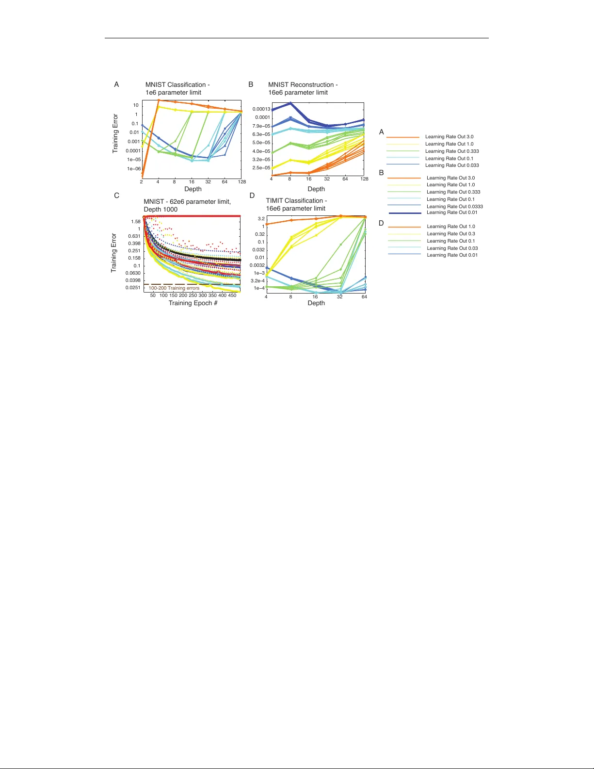
Under revie w as a conference paper at ICLR 2015 R A N D O M W A L K I N I T I A L I Z A T I O N F O R T R A I N I N G V E RY D E E P F E E D F O RW A R D N E T W O R K S David Sussillo Google Inc. Mountain V ie w , CA, 94303, USA sussillo@google.com L.F . Abbott Departments of Neuroscience and Physiology and Cellular Biophysics Columbia Univ ersity New Y ork, NY , 10032, USA lfabbott@columbia.edu A B S T R AC T T raining very deep networks is an important open problem in machine learning. One of man y dif ficulties is that the norm of the back-propagated error gradient can grow or decay exponentially . Here we show that training very deep feed-forwar d networks (FFNs) is not as difficult as previously thought. Unlike when back- propagation is applied to a recurrent network, application to an FFN amounts to multiplying the error gradient by a different random matrix at each layer . W e sho w that the successiv e application of correctly scaled random matrices to an initial vector results in a random walk of the log of the norm of the resulting vectors, and we compute the scaling that makes this walk unbiased. The variance of the random walk grows only linearly with network depth and is in v ersely proportional to the size of each layer . Practically , this implies a gradient whose log-norm scales with the square r oot of the network depth and shows that the v anishing gradient problem can be mitigated by increasing the width of the layers. Mathematical analyses and e xperimental results using stochastic gradient descent to optimize tasks related to the MNIST and TIMIT datasets are provided to support these claims. Equations for the optimal matrix scaling are provided for the linear and ReLU cases. 1 I N T RO D U C T I O N Since the early 90s, it has been appreciated that deep neural networks suffer from a vanishing gra- dient problem (Hochreiter, 1991), (Bengio et al., 1993), (Bengio et al., 1994), (Hochreiter et al., 2001). The term vanishing gradient refers to the fact that in a feedforward netw ork (FFN) the back- propagated error signal typically decreases (or increases) exponentially as a function of the distance from the final layer . This problem is also observed in recurrent networks (RNNs), where the errors are back-propagated in time and the error signal decreases (or increases) exponentially as a function of the distance back in time from the current error . Because of the v anishing gradient, adding man y extra layers in FFNs or time points in RNNs does not usually impro ve performance. Although it can be applied to both feedforward and recurrent networks, the analysis of the v anishing gradient problem is based on a recurrent architecture (e.g. (Hochreiter, 1991)). In a recurrent net- work, back-propagation through time in volv es applying similar matrices repeatedly to compute the error gradient. The outcome of this process depends on whether the magnitudes of the leading eigen- values of these matrices tend to be greater than or less than one 1 . Eigen value magnitudes greater than one produce exponential growth, and less than one produces e xponential decay . Only if the magnitude of the leading eigen values are tightly constrained can there be a useful “non-v anishing” 1 Excluding highly non-normal matrices. 1 Under revie w as a conference paper at ICLR 2015 gradient. Although this fine-tuning can be achieved by appropriate initialization, it will almost surely be lost as the optimization process goes forward. Interestingly , the analysis is very different for an FFN with randomly initialized matrices at each layer . When the error gradient is computed in a FFN, a dif ferent matrix is applied at every lev el of back-propagation. This small difference can result in a wildly dif ferent beha vior for the magnitude of the gradient norm for FFNs compared to RNNs. Here we show that correctly initialized FFNs suffer from the v anishing gradient problem in a far less drastic way than previously thought, namely that the magnitude of the gradient scales only as the square root of the depth of the network. Different approaches to training deep networks (both feedforward and recurrent) have been studied and applied, such as pre-training (Hinton & Salakhutdinov, 2006), better random initial scaling (Glorot & Bengio, 2010),(Sutskev er et al., 2013), better optimization methods (Martens, 2010), specific architectures (Krizhevsk y et al., 2012), orthogonal initialization (Saxe et al., 2013), etc. Further , the topic of why deep networks are difficult to train is also an area of active research (Glorot & Bengio, 2010), (Pascanu et al., 2012), (Sax e et al., 2013), (Pascanu et al., 2014). Here, we address the v anishing gradient problem using mathematical analysis and computational experiments that study the training error optimized deep-networks. W e analyze the norm of vectors that result from successi ve applications of random matrices, and we show that the analytical results hold empirically for the back-propagation equations of nonlinear FFNs with hundreds of layers. W e present and test a basic heuristic for initializing these networks, a procedure we call Random W alk Initialization because of the random walk of the log of the norms (log-norms) of the back- propagated errors. 2 A N A L Y S I S A N D P R O P O S E D I N I T I A L I Z A T I O N 2 . 1 T H E M A G N I T U D E O F T H E E R R O R G R A D I E N T I N F F N S W e focus on feedforward networks of the form a d = g W d h d − 1 + b d (1) h d = f ( a d ) , (2) with h d the vector of hidden activ ations, W d the linear transformation, and b d the biases, all at depth d , with d = 0 , 1 , 2 , . . . , D . The function f is an element-wise nonlinearity that we will normalize through the deri vati ve condition f 0 (0) = 1 , and g is a scale factor on the matrices. W e assume that the network has D layers and that each layer has width N (i.e. h d is a length N vector). Further we assume the elements of W d are initially drawn i.i.d. from a Gaussian distribution with zero mean and v ariance 1 / N . Otherwise the elements are set to 0. The elements of b d are initialized to zero. W e define h 0 to be the inputs and h D to be the outputs. W e assume that a task is defined for the network by a standard objecti ve function, E . Defining δ d ≡ ∂ E ∂ a   d , the corresponding back-propagation equation is δ d = g ˜ W d +1 δ d +1 , (3) where ˜ W d is a matrix with elements giv en by ˜ W d ( i, j ) = f 0 ( a d ( i )) W d ( j, i ) . (4) The e volution of the squared magnitude of the gradient v ector, | δ d | 2 , during back-propagation can be written as | δ d | 2 = g 2 z d +1 | δ d +1 | 2 , (5) where we hav e defined, for reasons that will become apparent, z d =    ˜ W d δ d / | δ d |    2 . (6) The entire ev olution of the gradient magnitude across all D layers of the netw ork is then described by Z = | δ 0 | 2 | δ D | 2 = g 2 D D Y d =1 z d , (7) 2 Under revie w as a conference paper at ICLR 2015 where we ha ve defined the across-all-layer gradient magnitude ratio as Z . Solving the v anishing gradient problem amounts to keeping Z of order 1, and our proposal is to do this by appropriately adjusting g . Of course, the matrices W and ˜ W change during learning, so we can only do this for the initial configuration of the network before learning has made these changes. W e will discuss how to mak e this initial adjustment and then sho w e xperimentally that it is suf ficient to maintain useful gradients ev en during learning. Because the matrices W are initially random, we can think of the z v ariables defined in equation (6) as random variables. Then, Z , giv en by equation (7), is proportional to a product of random variables and so, according to the central limit theorem for products of random variables, Z will be approximately log-normal distributed for large D . This implies that the distribution for Z is long- tailed. For applications to neural network optimization, we want a procedure that will re gularize Z in most cases, resulting in most optimizations making progress, b ut are willing to tolerate the occasional pathological case, resulting in a failed optimization. This means that we are not interested in catering to the tails of the Z distribution. T o avoid issues associated with these tails, we choose instead to consider the logarithm of equation (7), ln( Z ) = D ln( g 2 ) + D X d =1 ln( z d ) . (8) The sum in this equation means that we can think of ln( Z ) as being the result of a random walk, with step d in the walk gi ven by the random variable ln( z d ) . The goal of Random W alk Initialization is to chose g to make this walk unbiased. Equivalently , we choose g to make ln( Z ) as close to zero as possible. 2 . 2 C A L C U L A T I O N O F T H E O P T I M A L g V A L U E S Equation (8) describes the ev olution of the logarithm of the error-vector norm as the output-layer vector δ D is back-propagated through a network. In an actual application of the back-propagation algorithm, δ D would be computed by propagating an input forward through the network and com- paring the network output to the desired output for the particular task being trained. This is what we will do as well in our neural network optimization experiments, but we would like to begin by studying the vanishing gradient problem in a broader context, in particular , one that allo ws a general discussion independent of the particular task being trained. T o do this, we study what happens to randomly chosen vectors δ D when they are back-propagated, rather than studying specific vectors that result from forward propagation and an error computation. Among other things, this implies that the δ D we use are uncorrelated with the W matrices of the netw ork. Similarly , we want to make analytic statements that apply to all networks, not one specific network. T o accomplish this, we average over realizations of the matrices ˜ W applied during back-propagation. After present- ing the analytic results, we will show that they provide excellent approximations when applied to back-propagation calculations on specific networks being trained to perform specific tasks. When we average ov er the ˜ W matrices, each layer of the network becomes equiv alent, so we can write h ln( Z ) i = D  ln( g 2 ) + h ln( z ) i  = 0 , (9) determining the critical value of g as g = exp  − 1 2 h ln( z ) i  . (10) Here z is a random variable determined by z =    ˜ W δ / | δ |    2 , (11) with ˜ W and δ chosen from the same distribution as the ˜ W d and δ d variables of the dif ferent layers of the network (i.e. we hav e dropped the d index). W e will compute the optimal g of equation (10) under the assumption that ˜ W is i.i.d. Gaussian with zero mean. For linear networks, f 0 = 1 so ˜ W = W T , and this condition is satisfied due to the 3 Under revie w as a conference paper at ICLR 2015 definition of W . For the ReLU nonlinearity , f 0 effecti vely zeros out approximately half of the ro ws of ˜ W , but the Gaussian assumption applies to the non-zero ro ws. For the tanh nonlinearity , we will rely on numerical rather than analytic results and thus will not need this assumption. When ˜ W is Gaussian, so is ˜ W δ / | δ | , independent of the distribution or value of the vector δ (that is, the product of a Gaussian matrix and a unit v ector is a Gaussian v ector). The fact that ˜ W δ / | δ | is Gaussian for any vector δ means that we do not need to consider the properties of the δ d vectors at different network layers, making the calculations much easier . It also implies that z is χ 2 distributed because it is the squared magnitude of a Gaussian vector . More precisely , if the elements of the N × N matrix ˜ W hav e variance 1 / N , we can write z = η / N , where η is distributed according to χ 2 N , that is, a χ 2 distribution with N degrees of freedom. Writing z = η / N , expanding the logarithm in a T aylor series about z = 1 and using the mean and variance of the distrib ution χ 2 N , we find h ln( z ) i ≈ h ( z − 1) i − 1 2  ( z − 1) 2  = − 1 N . (12) From equation (10), this implies, to the same degree of approximation, that the optimal g is g linear = exp  1 2 N  . (13) The slope of the variance of the random w alk of ln( Z ) is given to this le vel of approximation by D (ln( z )) 2 E − D ln( z ) E 2 = 1 2 N . (14) Note that this is in versely proportional to N . These expressions are only computed to lowest order in a 1 / N expansion, b ut numerical studies indicate that the y are reasonably accurate (more accurate than expressions that include order 1 / N 2 terms) ov er the entire range of N values. For the ReLU case, ˜ W 6 = W T , b ut it is closely related because the factor of f 0 , which is equal to either 0 or 1, sets a fraction of the rows of ˜ W to 0 but leaves the other rows unchanged. Given the zero-mean initialization of W , both values of f 0 occur with probability 1/2. Thus the deriv ative of the ReLU function sets 1 − M rows of ˜ W to 0 and leaves M ro ws with Gaussian entries. The value of M is drawn from an N element binomial distribution with p = 1 / 2 , and z is the sum of the squares of M random variables with variance 1 / N . W e write z = η / N as before, but in this case, η is distributed according to χ 2 M . This means that z is a doubly stochastic variable: first M is drawn from the binomial distribution and then η is drawn from χ 2 M . Similarly , the average h ln( z ) i must now be done ov er both the χ 2 and binomial distributions. A complication in this procedure, and in using ReLU networks in general, is that if N is too small (about N < 20 ) a layer may hav e no activity in any of its units. W e remove these cases from our numerical studies and only av erage ov er nonzero values of M . W e can compute h ln( z ) i to leading order in 1 / N using a T aylor series as abo ve, but e xpanding around z = 1 / 2 in this case, to obtain h ln( z ) i ≈ − ln(2) − 2 N . (15) Howe ver , unlike in the linear case, this expression is not a good approximation ov er the entire N range. Instead, we computed h ln( z ) i and h (ln( z )) 2 i numerically and fit simple analytic expressions to the results to obtain h ln( z ) i ≈ − ln(2) − 2 . 4 max( N , 6) − 2 . 4 , (16) and D (ln( z )) 2 E − D ln( z ) E 2 ≈ 5 max( N , 6) − 4 . (17) From equation (16), we find g ReLU = √ 2 exp  1 . 2 max( N , 6) − 2 . 4  . (18) 4 Under revie w as a conference paper at ICLR 2015 Computing these av erages with the tanh nonlinearity is more difficult and, though it should be possible, we will not attempt to do this. Instead, we report numerical results below . In general, we should expect the optimal g v alue for the tanh case to be greater than g linear , because the deri vati ve of the tanh function reduces the variance of the rows of ˜ W compared with those of W , but less than g ReLU because multiple rows of ˜ W are not set to 0. 2 . 3 C O M P U TA T I O NA L V E R I FI C AT I O N The random walks that generate Z values according to equation (8) are shown in the top panel of Figure 1 for a linear network (with random vectors back-propagated). In this case, the optimal g value, gi ven by equation (13) was used, producing an unbiased random walk (middle panel of Figure 1). The linear increase in the variance of the random walk across layers is well predicted by variance computed in equation (14). 1 100 200 300 400 500 0 1 2 3 6 4 2 0 2 4 6 0.02 0 0.02 0.04 d  log( | δ d | ) 2   log( | δ d | )  log( | δ d | ) Figure 1: Sample random walks of random vectors back-propagated through a linear network. (T op) Many samples of random walks from equation (8) with N = 100 , D = 500 and g = 1 . 005 , as determined by equation (13). Both the starting v ectors as well as all matrices were generated randomly at each step of the random walk. (Middle) The mean o ver all instantiations (blue) is close to zero (red line) because the optimal g value w as used. (Bottom) The v ariance of the random w alks at layer d (blue), and the value predicted by equation (14) (red). W e also explored via numerical simulation the degree to which equations (10) and (18) were good approximations of the dependence of g on N . The results are sho wn in Figure 2. The top row of Figure 2 sho ws the predicted g value as a function of the layer width, N , and the nonlinearity . Each point is averaged over 200 random networks of the form giv en by equations (1-3) with D = 200 and both h 0 and δ D set to a random vectors whose elements hav e unit v ariance. The bottom row of Figure 2 shows the growth of the magnitude of δ 0 in comparison to δ D for a fixed N = 100 , as a function of the g scaling parameter and the nonlinearity . Each point is av eraged over 400 random instantiations of equations (1-2) and back-propagated via equations (3). The results show the predicted optimal g values from equations (13) and (18) match the data well, and they provide a numerical estimate of the optimal g value of the tanh case. In addition, we see that the range of serviceable values for g is larger for tanh than for the linear or ReLU cases due to the saturation of the nonlinearity compensating for growth due to g W d . 5 Under revie w as a conference paper at ICLR 2015 Linear Linear ReLU ReLU Tanh Tanh g g g N N N g 20 40 60 80 100 120 140 160 180 200 1.005 1.01 1.015 1.02 1.025 20 40 60 80 100 120 140 160 180 200 1.43 1.44 1.45 1.46 1.47 1.48 1.49 1.5 1.51 20 40 60 80 100 120 140 160 180 200 1.1 1.15 1.2 1.25 1.3 1.35 0.995 1 1.005 1.01 1.015 −1.5 −1 −0.5 0 0.5 1 1.5 2 1.424 1.428 1.432 1.436 1.44 −1 −0.5 0 0.5 1 1 1.05 1.1 1.15 1.2 1.25 −4 −3 −2 −1 0 1 2  log( | δ 0 | | δ D | )  Figure 2: T op - Numerical simulation of the best g as a function of N , using equations (1-3) using random vectors for h 0 and δ D . Black shows results of numerical simulations, and red shows the predicted best g values from equations (13) and (18). (Left) linear, (Middle) - ReLU , (Right) - tanh . Bottom - Numerical simulation of the average log( | δ 0 | / | δ D | ) as a function of g , again using equations (1-3). Results from equations (13) and (18) are indicated by red arrows. Guidelines at 0 (solid green) and -1, 1 (dashed green) are provided. 3 R E S U L T S O F T R A I N I N G D E E P N E T W O R K S W I T H R A N D O M W A L K I N I T I A L I Z A T I O N 3 . 1 R A N D O M W A L K I N I T I A L I Z A T I O N The general methodology used in the Random W alk Initialization is to set g according to the values giv en in equations (13) and (18) for the linear and ReLU cases, respectively . For tanh , the values between 1.1 and 1.3 are sho wn to be good in practice, as sho wn in Figure 2 (upper right panel) and in Figure 3 (left panels). The scaling of the input distribution itself should also be adjusted to zero mean and unit variance in each dimension. Poor input scaling will effect the back-propagation through the deriv ativ e terms in equation (3) for some number of early layers before the randomness of the initial matrices “w ashes out” the poor scaling. A slight adjustment to g may be helpful, based on the actual data distribution, as most real-world data is far from a normal distribution. By similar reasoning, the initial scaling of the final output layer may need to be adjusted separately , as the back-propagating errors will be affected by the initialization of the final output layer . In summary , Random W alk Initialization requires tuning of three parameters: input scaling (or g 1 ), g D , and g , the first two to handle transient ef fects of the inputs and errors, and the last to generally tune the entire network. By far the most important of the three is g . 3 . 2 E X P E R I M E N TA L M E T H O D S T o assess the quality of the training error for deep nonlinear FFNs set up with Random W alk Initial- ization, we ran experiments on both the MNIST and TIMIT datasets with a standard FFN defined by equations (1-2). In particular we studied the classification problem for both MNIST and TIMIT , using cross-entrop y error for multiclass classification, and we studied reconstruction of MNIST dig- its using auto-encoders, using mean squared error . For the TIMIT study , the input features were 15 frames (+/- 7 frames of context, with ∆ and ∆∆ ). In these studies, we focused exclusi vely on train- ing error, as the ef fect of depth on generalization is a different problem (though obviously important) from how one can train deep FFNs in the first place. 6 Under revie w as a conference paper at ICLR 2015 The general experimental procedure w as to limit the number of parameters, e.g. 4e6 parameters, and distribute them between matrices and biases of each layer in a network. The classification experiments used constant width layers, and for these experiments the actual number of parameters was the first value abo ve the parameter limit, p lim , such that a constant integer value of N was possible. Thus as a network got deeper , its layers also became more narrow . For example, for the MNIST dataset, at p lim = 4 e 6 , for D = 4 , N = 1228 and for D = 512 , N = 88 . For the MNIST auto-encoder experiments, p lim = 16 e 6 , and the code layer was 30 linear units. The size of each layer surrounding this middle encoding layer was chosen by picking a constant increase in layer size such that the total number of parameters was first number above p lim that led to an integral layer width for all layers. For example, at D = 4 , the layer sizes were [9816 30 9816 784] , while for D = 128 the layer sizes were [576 567 558 ... 48 39 30 38 48 ... 558 567 576 784] . In these auto-encoder studies we used the tanh nonlinearity , and v aried the g parameter per experiment, but not per layer . Our experiments compared one depth to another so we v aried the learning rates quite a bit to ensure fairness for both shallow and deep networks. In particular , we varied the minimal and maximal learning rates per e xperiment. In essence, we had an exponential learning rate schedule as a function of depth , with the minimal and maximal values of that exponential set as hyper-parameters. More precisely , we denote the maximum depth in an experiment as D max (e.g. if we compared networks with depths [4 8 16 32 64 128] in a single experiment, then D max = 128 ). Let λ in and λ out be the learning rate hyper -parameters for the input and output layers, respectively . The exponential learning rate schedule with decay τ and scale α , as a function of depth, took the form τ = ( D max − 1) ln( λ out ) − ln( λ in ) (19) α = exp(ln( λ in ) + D max τ ) (20) γ d = α exp( − D max − d + 1 τ ) . (21) Then for a given network with depth D , potentially smaller than D max , the learning rates were set for the actual experiment as λ D − d = γ D max − d . (22) A key aspect of this learning rate scheme is that shallo wer networks are not ov erly penalized with tiny learning rates in the early layers. This is because the decay starts with layer D getting learning rate λ out and goes backwards to the first layer , which gets a learning rate λ D max − D . This means that for networks more shallow than D max , λ 1 could be much larger than λ in ; only if D = D max did λ 1 = λ in . Some experiments had λ in < λ out , some had λ in > λ out , and we also tested the standard λ in = λ out (no learning rate schedule as a function of depth for all experiments). For the very deep networks, varying the learning rates as a function of depth was very important, although we do not study it in depth here. Finally , the learning rates in all layers were uniformly decayed by a multiplicativ e factor of 0.995 at the end of each training epoch. Beyond setting learning rate schedules, there were no bells and whistles. W e trained the networks using standard stochastic gradient descent (SGD) with a minibatch size of 100 for 500 epochs of the full training dataset. W e also used gradient clipping, in cases when the gradient became very large, although this w as very uncommon. The combination of hyper -parameters: the varied learning rates, depths, and g v alues resulted in roughly 300-1000 optimizations for each panel displayed in Figure 3 and Figure 4. 3 . 3 P E R F O R M A N C E R E S U L T S W e employed a first set of experiments to determine whether or not training a real-world dataset would be affected by choosing g according to the Random W alk Initialization. W e trained many networks as described abo ve on the MNIST dataset. The results are shown in Figure 3 for both the tanh and ReLU nonlinearities. Namely , for tanh the smallest training error for most depths is between g = 1 . 1 and g = 1 . 4 , in good agreement with Figure 2 (upper left panel). For ReLU the smallest training error was between g = 1 . 4 and g = 1 . 55 . These results are in very good agreement with our analytic calculations and the results shown in Figure 2 (upper middle panel). 7 Under revie w as a conference paper at ICLR 2015 0.9 1 1.1 1.2 1.3 1.4 1.5 1.6 1.7 0.001 0.0032 0.01 0.032 0.1 0.32 1 g Training Error 0.9 1 1.1 1.2 1.3 1.4 1.5 1.6 1.7 0.001 0.0032 0.01 0.032 0.1 0.32 1 g Training Error 1.25 1.3 1.35 1.4 1.45 1.5 1.55 1.6 1.65 3.2e−05 0.0001 0.00032 0.001 0.0032 0.01 0.032 0.1 0.32 1 g 1.25 1.3 1.35 1.4 1.45 1.5 1.55 1.6 1.65 0.0001 0.001 0.01 0.1 1 10 g depth = 64 depth = 128 depth = 256 depth = 512 depth = 32 depth = 64 depth = 128 depth = 256 T anh - Error across all learning rates ReLU - Error across all learning rates T anh - Error (min of learning rates) ReLU - Error (min of learning rates) Figure 3: Training error on MNIST as a function of g and D . Each simulation used a parameter limit of 4 e 6 . Error sho wn on a log 10 scale. The g parameter is varied on the x-axis, and color denotes v arious values of D . (Upper left) T raining error for the tanh function for all learning rate combinations. The learning rate hyper-parameters λ in and λ out are not visually distinguished. (Lower left) Same as upper left e xcept showing the minimum training error for all learning rate combinations. (Upper right and lower right) Same as left, b ut for the ReLU nonlinearity . For both nonlinearities, the experimental results are in good agreement with analytical and e xperimental predictions. The goal of the second set of experiments was to assess training error as a function of D . In other words, does increased depth actually help to decrease the objectiv e function? Here we focused on the tanh nonlinearity as many believ e ReLU is the easier function to use. Having demonstrated the utility of correctly scaling g , we used a variety of g values in the general optimal range abo ve 1. The results for MNIST classification are shown in Figure 4A. The best training error was depth 2, with a very large learning rate. T ied for second place, depths of 16 and 32 showed the next lowest training error . The MNIST auto-encoder experiments are shown in Figure 4B. Again the most shallow network achieved the best training error . Ho wever , ev en depths of 128 were only roughly 2x greater in training error , thus demonstrating the effecti veness of our initialization scheme. Mostly as a stunt, we trained networks with 1000 layers to classify MNIST . The parameter limit was 62e6, resulting in a layer width of 249. The results are shown in Figure 4C. The very best networks (over all hyper-parameters) were able to achiev e a performance of about 50 training mistakes. W e also tried Random W alk Initialization on the TIMIT dataset (Figure 4D) and the results were similar to MNIST . The best training error among the depths tested w as depth 16, with depth 32 essentially tied. In summary , depth did not improv e training error on any of the tasks we examined, but these experiments nev ertheless provide strong evidence that our initialization is reasonable for very deep nonlinear FFNs trained on real-world data. 8 Under revie w as a conference paper at ICLR 2015 50 100 150 200 250 300 350 400 450 0.0251 0.0398 0.0630 0.1 0.158 0.251 0.398 0.631 1 1.58 MNIST - 62e6 parameter limit, Depth 1000 T raining Error T raining Error MNIST Classification - 1e6 parameter limit MNIST Reconstruction - 16e6 parameter limit TIMIT Classification - 16e6 parameter limit T raining Epoch # Depth Depth Depth Learning Rate Out 3.0 Learning Rate Out 1.0 Learning Rate Out 0.333 Learning Rate Out 0.1 Learning Rate Out 0.033 A A B C D Learning Rate Out 3.0 Learning Rate Out 1.0 Learning Rate Out 0.333 Learning Rate Out 0.1 Learning Rate Out 0.0333 B D 2 4 8 16 32 64 128 1e−06 1e−05 0.0001 0.001 0.01 0.1 1 10 4 8 16 32 64 128 2.5e−05 3.2e−05 4.0e−05 5.0e−05 6.3e−05 7.9e−05 0.0001 0.00013 Learning Rate Out 0.01 4 8 16 32 64 1e−4 3.2e-4 1e−3 0.0032 0.01 0.032 0.1 0.32 1 3.2 Learning Rate Out 1.0 Learning Rate Out 0.3 Learning Rate Out 0.1 Learning Rate Out 0.03 Learning Rate Out 0.01 100-200 T raining errors Figure 4: Performance results using Random W alk Initialization on MNIST and TIMIT . Each net- work had the same parameter limit, regardless of depth. T raining error is shown on a log 2 − log 10 plot. The legend for color coding of λ out is shown at right. The values of λ in were varied with the same values as λ out and are shown with different markers. V aried g values were also used and av- eraged ov er . For A and B, g = [1 . 05 , 1 . 1 , 1 . 15 , 1 . 2] . (A) The classification training error on MNIST as a function of D , λ in and λ out . (B) MNIST Auto-encoder reconstruction error as a function of hyper-parameters. (C) Experiments on MNIST with D = 1000 . Training error is shown as a func- tion of training epoch. Hyper-parameters of λ in , λ out , were varied to get a sense of the difficulty of training such a deep network. The v alue of g = 1 . 05 was used to combat pathological curv ature. (D) Classification training error on TIMIT dataset. V alues of g = [1 . 1 , 1 . 15 , 1 . 2 , 1 . 25] were averaged ov er . 4 D I S C U S S I O N The results presented here imply that correctly initialized FFNs, with g v alues set as in Figure 2 or as in equation (13) for linear networks and equation (18) for ReLU networks, can be successfully trained on real datasets for depths upwards of 200 layers. Importantly , one may simply increase N to decrease the fluctuations in the norm of the back-propagated errors. W e deriv ed equations for the correct g for both the linear and ReLU cases. While our experiments explicitly used SGD and av oided regularization, there is no reason that Random W alk Initialization should be incompatible with other methods used to train very deep netw orks, including second-order optimization, dif ferent architectures, or regularization methods. This study revealed a number of points about training very deep networks. First, one should be careful with biases. Throughout our experiments, we initialized the biases to zero, though we al ways allowed them to be modified. For the most part, use of biases did not hurt the results. Howe ver , care must be taken with the learning rates because the optimization may use the biases to quickly match the target mean across e xamples. If this happens, the careful initialization may be destroyed and forward progress in the optimization will cease. Second, learning rates in very deep networks are very important. As can be seen from Figure 4D (e.g. D = 32 ), the exact learning rate scheduling made a huge dif ference in performance. Third, we suspect that for extremely deep networks (e.g. 1000 layers as in Figure 4C), curvature of the error landscape may be extremely problematic. This means that the network is so sensitive to changes in the first layer that effecti ve optimization of the 9 Under revie w as a conference paper at ICLR 2015 1000 layer network with a first-order optimization method is impossible. Indeed, we set g = 1 . 05 in Figure 4C precisely to deal with this issue. Our e xperimental results show that ev en though depth did not clearly impro ve the training error , the initialization scheme was ne vertheless ef fectiv e at allo wing training of these very deep netw orks to go forw ard. Namely , almost all models with correctly chosen g that were not brok en, due to a mismatch of learning rate hyper-parameters to architecture, reached zero or near-zero training classification error or extremely low reconstruction error, regardless of depth. Further research is necessary to determine whether or not more difficult or different tasks can make use of very deep feedforward networks in a way that is useful in applied settings. Regardless, these results sho w that initializing v ery deep feedforward networks with Random W alk Initialization, g set according to Figure 2 or as described in the section Calculation of the Optimal g V alues , as opposed to g = 1 , is an easily implemented, sensible default initialization. A C K N O W L E D G M E N T S W e thank Quoc Le and Ilya Sutskev er for useful discussions. R E F E R E N C E S Bengio, Y ., Frasconi, P ., and Simard, P . The problem of learning long-term dependencies in recurrent networks. pp. 1183–1195, San Francisco, 1993. IEEE Press. (invited paper). Bengio, Y ., Simard, P ., and Frasconi, P . Learning long-term dependencies with gradient descent is difficult. 5(2):157–166, 1994. Glorot, Xavier and Bengio, Y oshua. Understanding the dif ficulty of training deep feedforward neural networks. In International Conference on Artificial Intelligence and Statistics , pp. 249–256, 2010. Hinton, Geoffrey E and Salakhutdinov , Ruslan R. Reducing the dimensionality of data with neural networks. Science , 313(5786):504–507, 2006. Hochreiter , S. Untersuchungen zu dynamischen neuronalen Netzen. Diploma thesis, T .U. M ¨ unich, 1991. Hochreiter , Sepp, Bengio, Y oshua, Frasconi, Paolo, and Schmidhuber , J ¨ urgen. Gradient flo w in recurrent nets: the difficulty of learning long-term dependencies, 2001. Krizhevsk y , Alex, Sutskev er , Ilya, and Hinton, Geof frey E. Imagenet classification with deep con vo- lutional neural networks. In Advances in neural information processing systems , pp. 1097–1105, 2012. Martens, James. Deep learning via hessian-free optimization. In Pr oceedings of the 27th Interna- tional Confer ence on Machine Learning (ICML-10) , pp. 735–742, 2010. Pascanu, Razv an, Mikolo v , T omas, and Bengio, Y oshua. On the difficulty of training recurrent neural networks. arXiv pr eprint arXiv:1211.5063 , 2012. Pascanu, Razvan, Dauphin, Y ann N, Ganguli, Surya, and Bengio, Y oshua. On the saddle point problem for non-con vex optimization. arXiv preprint , 2014. Saxe, Andrew M, McClelland, James L, and Ganguli, Surya. Exact solutions to the nonlinear dy- namics of learning in deep linear neural networks. arXiv pr eprint arXiv:1312.6120 , 2013. Sutske ver , Ilya, Martens, James, Dahl, George, and Hinton, Geoffrey . On the importance of initial- ization and momentum in deep learning. In Pr oceedings of the 30th International Conference on Machine Learning (ICML-13) , pp. 1139–1147, 2013. 10