Downlink Scheduling over Markovian Fading Channels

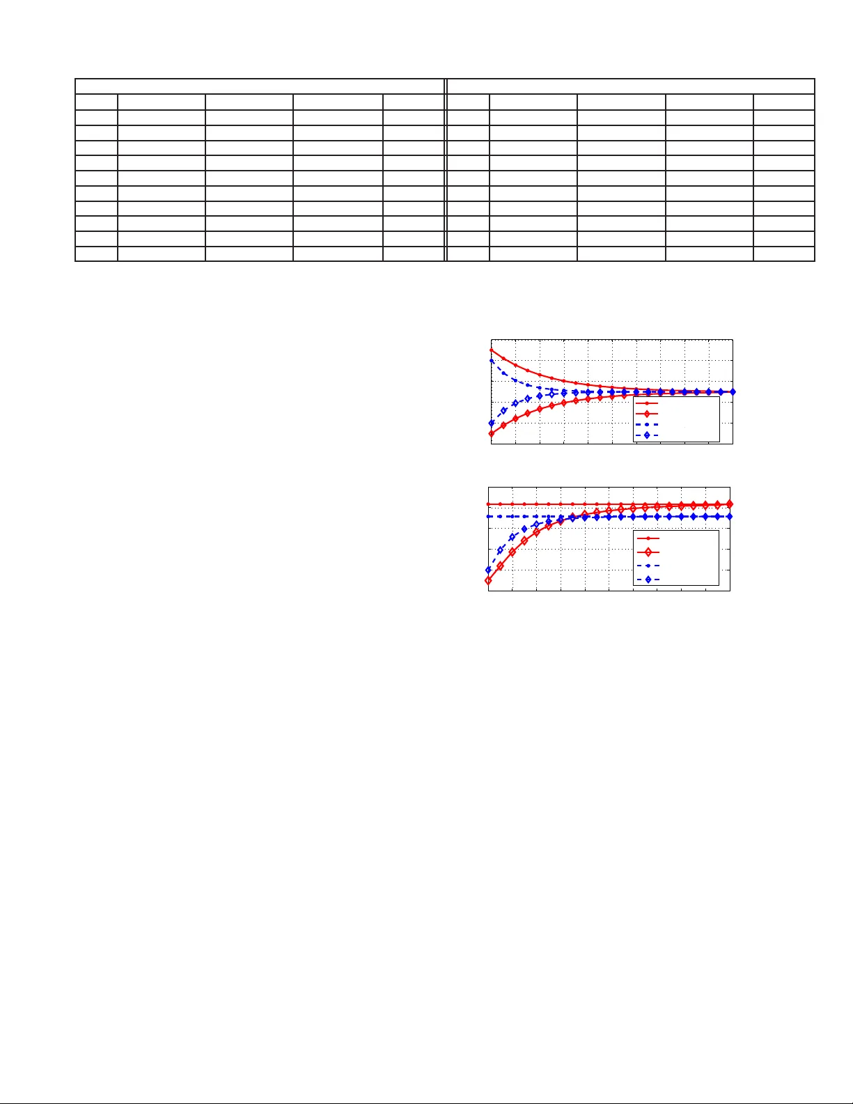
1 Do wnlink Scheduling o ver Mar ko vian F ading Channels W enzhuo Ouyang, Atilla Eryilmaz, and Ness B. Shr off Abstract —W e consider the scheduling problem in downlink wireless networks wit h heterogeneous, Markov- modulated, ON/OFF channels. It is we ll-known tha t the performance of scheduling ov er fa ding cha nnels relies heavily on the accuracy of the available Channel State Inf ormation (CSI), which is co stly to acquire. Thus , we consider the CSI a cquisition via a pra ctical ARQ-based feedback mechanism whereby c hannel states are revealed at the end of only scheduled users’ transmissions. In the assumed presence of temporally-co rrelated channel evolutions, the desired scheduler must opt imally balance the explo itation-explo ration trade-off , whereby it schedules transmissions bo th t o e xploit tho se channels with up-to- date CSI and to ex plore t he current stat e of those with outdated CSI. In earlier works, Whittle’ s Index Policy h ad been suggested as a low-complexity and high- performance solution to t his problem. However , analyzing its perfor- mance in the typical scenario of sta tistically heteroge- neous channel state processes has remained elusive and challenging, mainly because of the highly-coupled and complex dynamics it possesses. In this work, we overcome these difﬁculties t o rigo rously esta blish the a symptotic optimality properties o f Whittle’s Index Policy in the limiting regime of many users. More s peciﬁcally: (1 ) we prove the local op timality of Whitt le’ s Index Policy , provided that the initial sta te o f the system is within a certain neighborhood of a carefully selected state; (2) we then esta blish the g lobal optimality of Whittle ’ s Index Policy under a recurrence assumption that is veriﬁed numerically f or o ur pr o blem. These results establish that Whittle’ s Index Policy possesses analy tically provable op- timality char acteristics f or scheduling over heterogeneous and temporally -correlated channels. W enzh uo Ouyang and Atilla Eryil maz are with the Department of ECE, The Ohio S tate Univ ersity ( e-mails: ouyangw@ece.osu.ed u, eryilmaz@ece.osu.edu). Ness B. Shro ff holds a joint appointment in both the Department of ECE and the Department of CSE at The Ohio State Univ ersi ty (e-mail: shro ff@ece .osu.edu). A preliminary version of this paper appeared in INFOCOM 2012. This work was supported in part by NSF grants CAREER- CNS-0953515, CCF-091666 4, CNS-1012700, DTRA grant HDTRA 1-08-1-001 6, Qatar National Research Fund (QNRF) under the National Prioriti es Research Program (NP RP) grant NPRP 09-1168- 2-455, and ARO MURI a ward W 911NF-08-1-023 8. I . I N T RO D U C T I O N Channel ﬂuctuation is a n intrinsic characteristic of wireless communications. Such a variation ca lls for allocation of the wireless resources in a dynamic man- ner , leading to the classic opportunistic scheduling principle (e.g., [1][2]). Unde r the assump tion that the instantaneou s c hanne l s tate information (CSI) is fully av ailable to the sched uler , many efﬁcient opportunistic schedu ling algorit hms (e.g., [4]-[6]) ha ve been proposed and extens i vely studied . More recent works ha ve focused on designing schedu ling algo rithms under i mperfect CSI, where the channe l state is mo deled as independ ent a nd identi- cally distrib uted ( i.i.d. ) p rocesse s a cross time (e.g., [9]- [13]). On the othe r han d, although the i.i.d. c hanne l model brings ease of ana lysis, it fails to cap ture the time-correlation of the fading channels [3]. Spec iﬁ- cally , it fails to exploit the channe l memory , which is a critical res ource for making sche duling decisions. Howe ver , designing ef ﬁ cient scheduling schemes under time-correlated ch annels with imperfect CSI is a very challenging problem. The challeng e is mainly because of the dif ﬁcu lty i n making the classic ‘exploitati on versus exploration’ trade-of f (e.g., [7], [8]), in which a sch eduler need s to strike a balance betwee n selecting the chan nels with up-to-date chan nel memory that guar- antees h igh immed iate gains, or to exp lore the channels with outdated CSI for more informed decision s and assoc iated future throughput g ains. W e consider the downlink schedu ling problem w here a base s tation transmits to the users within its transmis- sion range , sub ject to sched uling constraints. T o mod el the time c orrelations presen t over f ading channe ls, we assu me that wireless channe ls evol ve as Markov- modulated ON/OFF processes. Th e c hanne l state in- formation is obtained from ARQ-based fee dback, on ly after e ach sched uled trans mission. Nev ertheless, due to time correlation, the memory of the past channel s tate can be u sed to predict the current channe l state prior to sche duling decision. Hence, channe l memory should be intelligently exploited by the s chedu ler in order to achieve high throug hput performanc e. 2 In a related work [14], a similar problem is con- sidered unde r delaye d CSI, where it is assume d that perfect CS I is av ailable within a ma ximum delay , which is in turn smaller than the delay experienced by the ARQ feedba ck used for collision detec tion. These as sumptions allow the scheduling decision s to be decoupled fr o m CSI acquisition, which leads to the development of centralized as well as distributed schedu lers. Howe ver , this approach d oes no t us e ARQ as a means of acquiring impro ved channel quality information. In con trast, in our s etup the nature of ARQ feedba ck creates a n implicit impa ct of schedu l- ing dec isions on the CSI feed back, which comp letely transforms the nature of the optimal scheduler design, and therefore requires a different approach. Under the scena rio where all the c hanne ls have identical Mar kov statistics , round-robin-bas ed algorit h ms (e.g., [15]-[18]) have be en shown to pos sess op timality properties in throughput performance. Ho wev er , the round-robin- based algorithms are no longer optimal in asym metric scenar ios , e.g., when dif ferent channe ls ha ve dif feren t Markov t ransition statistics, as is naturally the cas e in typical h eterogeneo us c onditions. Under the asymmetric scenarios, our downlink schedu ling prob lem i s an example of the classic Re st- less Multiarmed Band it Problem (RMBP) [19]. Low- complexity Whittle’ s Index Policies [19] for the down- link scheduling problem ha ve been proposed in [20][21] based on R MBP theory . Howe ver , although Whittle’ s Index Policy can bring signiﬁcant throughput gains by exploiting the chann el memory [21], the ana lytical characterization o f its performanc e under asymmetric scena rios i s very challenging and prohibiti vely techni- cal. This is becaus e a symmetry leads to a sophisticated interplay of memory e voluti on a mong chann els with heterogene ous chara cteristics, which brings a signiﬁ- cant challenge to the an alysis of Whittl e’ s Index Policy not pre sent in the perfectly symmetric s cenario. For RMBP problems unde r general scenarios, Whit- tle’ s Index Policy has been proven in [22] to be asymptotically optimal a s the number o f u sers grows, provided a non-tri vial con dition, known as W eber’ s condition, holds. Nonethe less, W eber’ s condition con - cerns the g lobal con ver g ence of a no n-linear differential equation, which is extremely dif ﬁcult to verify ev e n numerically in our downlink sc heduling scenario. In [23], optimality properties of gen eral RMBP is s tudied, where a sub-optimal BALANCED-INDEX policy , as well as a THRESHOLD-WHITTLE policy , are proved to provide 2 − ap proximation performance , i.e., ac hiev es at least half of the optimal rew a rd. Our work takes a dif fere nt a pproach than [23] to speciﬁcally study the per-user throu ghput performance of the Whittle’ s Index Policy for d ownlink sche duling, an d consider the strict optimality metric in the as ymptotic regime when the number of users scales. In this pa per , we take signiﬁcant steps in a nalyzing the optimality properties of Whitt le’ s Index Polic y for the downli nk scheduling prob lem in the prese nce o f channe l h eterogene ity . Spe ciﬁcally , o ur contrib utions are as f ollo ws. • W e a pply the Wh ittle’ s index framework to our downlink sc heduling prob lem and identify the optimal policy for the problem with a relaxed constraint in Section I II. This policy , with carefully selected randomization, provides a pe rformance upper bo und to Whittle’ s Index Policy . • W e establish the local optimality of Whittle’ s Index Policy in the as ymptotic regime when the number of users s cales in Section V. Sp eciﬁcally , we show that the p erformance of the index policy can get arbitrarily clos e to that of the relaxed-co nstraint optimal policy , provided that the initial state of the system is within a certain neighb orhood of a carefully s elected state. • Based on the local op timality result, und er a numerically veriﬁable recurrence assu mption, we then establish the glob al op timality of Whittle’ s Index Po licy in the limiti ng regime o f many use rs in Sec tion VI. I I . S Y S T E M M O D E L A N D P R O B L E M F O R M U L AT I O N A. Downlink W ir e less Channe l Model W e co nsider a ti me-slotted, wireless downlink sys tem with one base stati on and N users. The wir e less chan nel C i [ t ] between base station and user i remains static within eac h time slot t and evolv e s stochas tically across time slots, independently acros s users. W e adopt the simplest non-trivial model of time-correlated f a ding channe ls by cons idering two-state ON/OFF channels, where the state space of c hanne l i is S i = { 0 , 1 } , with the value of e ach state rep resenting the transmission rate a channel can su pport at the state. One important co mponent of our mode l is the in- clusion o f ch annel heteroge neity that the users will typically experience in real systems . Su ch asymme try creates a signiﬁcant c hallenge to the design and a nalysis of op timal sch eduling sch emes compared to perfectly symmetric channe ls. T o av oid cumbersome notation and unes sential technica l c omplications, in this work we model c hannel asymmetry by considering only two classes o f channel statistics. Spec iﬁcally , for all 3 0 k p k r k r − 1 k p − 1 1 Fig. 1 : T w o s tate Mark ov chain model for channels i n class k . the channels in clas s k , k = 1 , 2 , their states e volve according to the same Markov statistics. Howev e r , these ch aracteristics differ between classes. The state transition of ch annels in clas s k is depicted in Fig. 1, represented by a 2 × 2 probability trans ition matrix, P k =  p k 1 − p k r k 1 − r k  , where p k := prob  C i [ t ]=1   C i [ t − 1]=1  , r k := prob  C i [ t ]=1   C i [ t − 1]=0  . for chan nel i in class k . The number of clas s k chann els is γ k N , k ∈ { 1 , 2 } with γ k being the p r opo rtion of channe ls in class k with respe ctiv e to the total numbe r N of chan nels. W e study the scena rio where all the Markovian channe ls are pos iti vely co rrelated, i.e., p k > r k for k =1 , 2 . This a ssumption, which is commonly made in this doma in (e.g., [17], [18], [24]) , mea ns that the c han- nel ev olution ha s a positiv e auto-correlation. He nce, roughly speak ing, the ch annel has a stronger potential to stay in its previous state than jumping to another , which is typ ical especia lly in slow f a ding en vironme nt. For ea se of exposition, we sha ll exclude the trivi al case when r k = 0 or p k = 1 , k = 1 , 2 . B. Scheduling Model – Belief V alue Evolution W e as sume tha t the b ase station can simultaneo usly transmit to at mos t αN ∈ Z + users in a ti me slot without interference, wh ere α ∈ (0 , 1] stands for the maximum fraction of us ers tha t can be activ ated. For example, in a multi-channel communication model, α would corresp ond to the fraction of a ll us ers tha t can be simultaneo usly serviced in unit time. Howe ver , the schedu ler doe s no t k now the exact chann el state in the c urrent slot when the sc heduling decis ion is made. Instead, the sc heduler maintains a belief value π i [ t ] for e ach channel i , which is deﬁned as the probability of chann el i being in the ON state at the beginning of slot t . The accurate channel state is revealed via A CK/N ACK feed back from the sche duled us ers, only at the end of each time slot after the da ta is transmitted. This accurate chann el state fee dback is in turn used by the sch eduler to up date the belief v alues. For us er i in c lass k , k = 1 , 2 , let a i [ t ] ∈{ 0 , 1 } indicate whether the user is selected f or transmission in slot t . Then, from the d eﬁnition the be lief values, π i [ t ] ev olves as follows, π i [ t +1]=      p k , if a i [ t ]=1 , C i [ t ]=1 , r k , if a i [ t ]=1 , C i [ t ]=0 , π i [ t ] p k +(1 − π i [ t ]) r k , if a i [ t ]=0 . (1) In our se tup, belief values are known to be sufﬁcient statistics to r e present the past s chedu ling de cisions and feedback (e.g., [16], [25]). In the meanwh ile, in our ON/OFF chann el mode l, π i [ t ] also equa ls to the expected throughpu t contributed b y ch annel i if it is schedu led in time slot t . For a user in class k , k =1 , 2 , we use b k c,l to denote its belief value whe n the most recent observed channe l was c ∈ { 0 , 1 } , and is l slots in the pa st. From the belief update rule ( 1 ), b k c,l can be calculated a s a func tion of l ≥ 1 as, b k 0 ,l = r k − ( p k − r k ) l r k 1 + r k − p k , b k 1 ,l = r k + (1 − p k )( p k − r k ) l 1 + r k − p k . Fig. 2 illustrates the b elief value upd ate when a channe l s tays idle (i.e., a i =0 ). It is clear tha t if the schedu ler is never updated of the state of c hannel i (in class k ), the belief value will c on verge to its stationary probability of being ON, de noted by the s tationary belief value b k s := r k / (1+ r k − p k ) . The vector ~ π [ t ]=( π 1 [ t ] , · · · , π N [ t ]) denotes the belief values of all channels at the beginning of slot t . W e use B k to represe nt the s et of the belief values for class k channels , whe re B k = { b k s , b k c,l , c ∈ { 0 , 1 } , l ∈ Z + } . W e assume that the sys tem starts to operate from slot t = 0 . At the beginning of s lot 0 , for each channel the schedu ler has either observed its channel state be fore, or has never been updated of its c hanne l state, i.e., w ith belief value b k s . It is then clear that, based on the b elief update rule (1), π i [ t ] ∈ B k for a ll t ≥ 0 , i.e ., e ach be lief value π i [ t ] e volves over countab ly many s tates. In the rest of the pap er , we shall use ‘belief value’ and ‘belief state’ interchangea bly . C. Downlink Schedu ling Pr oblem – POMDP F ormula- tion W e cons ider the broad class U of (po ssibly n on- stationary) sch eduling policies that makes a schedu ling 4 1 2 3 4 5 6 7 8 9 10 0 0.2 0.4 0.6 0.8 1 Time of staying idle: l Belief value b k 1,l b k 0,l Fig. 2 : Belief values u pdate whe n staying idle, p k = 0 . 8 , r k = 0 . 2 , b k s = 0 . 5 . decision based on t he history of observed chan nel states and s chedu ling actions . Th e d ownlink sch eduling problem is then to identify a policy in U t h at maximizes the inﬁnite ho rizon, time average expected thr oughpu t , subject to the con straint on the number of users se lected at each time slot. Gi ven the initial state ~ π [0] , the problem is for mulated as, max u ∈ U lim inf T →∞ 1 T E h T − 1 X t =0 N X i =1 π i [ t ] · a u i [ t ]    ~ π [0] i (2) s.t. N X i =1 a u i [ t ] ≤ αN , ∀ t. (3) where the belief value π i [ t ] ev o lves acc ording to rule (1) based on the sch eduling decision a u i [ t ] under policy u . Such an o bjectiv e is s tandard in literature for Markov Decision Processe s u nder the long term a verage re ward criteria (e.g., [26 ]). No ting that sinc e the sche duling decisions are made b ased on i ncomplete knowledge of channe l states, this problem is a Partially Obs ervable Markov Decision Process [25]. This problem is in f a ct an example of Restless Mul- tiarmed Bandit Problem (RMBP) [19]. For a general RMBP , ﬁn ding a n op timal so lution is P SP A C E-hard [27]. Howev er , for the downlink sch eduling problem at ha nd, a low- complexity Whittle’ s Index Policy was proposed in [20][21] based on the RMBP theory that inherently exploits the c hanne l memory wh en making schedu ling decision s. For de tailed d escriptions o f g en- eral RMBP and Whittle’ s Index Po licy for do wnlink schedu ling, p lease refer to [19]-[21]. For the d ownlink sched uling problem, we note tha t there is only limited analytical ch aracterization of Whittle’ s Index Policy , which is restricted in perfectly symmetric scen arios where Whittle’ s Index Po licy t akes a spec ial round-robin form [20]. In asymme tric cases, howe ver , the sc heduling decision no longer takes the form of round-robin, b ringing sophisticated complica- tions in belief value evoluti ons that are tightly coupled among ch annels, which signiﬁcantly comp licates the analysis. The main focu s of this p aper is to analytically characterize the performanc e of Whittl e’ s Index Policy in the asymmetric case with tw o classes of channels. I I I . U P P E R B O U N D O N A C H I E V A B L E T H R O U G H P U T W e begin our analysis by characterizing a n upper bound to the through put performance of all feasible downlink sched uling policies that satisﬁes the constraint (3). The upper bound i s obtained from a ﬁctitious policy which is optimal for the downlink schedu ling problem under a r elaxed con straint . Note here that such relaxation is also a crucial s tep in the s tudy of the ge neral RMBP problem. Y et, our analysis, being spec iﬁc to the downlink s cheduling problem, has its novelties, a s we sha ll remark on later . A. A ve rage-Constrained Relaxed Scheduling Pr ob lem W e consider an as sociated relaxed p roblem o f (2)- (3) that only requires a n average number of users to be activ ated in the long run, deﬁned as follows max u ∈ U lim inf T →∞ 1 T E h T − 1 X t =0 N X i =1 π i [ t ] · a u i [ t ]    ~ π [0] i (4) s.t. lim sup T →∞ 1 T E h T − 1 X t =0 N X i =1 a u i [ t ] i ≤ αN . (5) Note that, contrary to the stringent constraint (3), the relaxed constraint (5) a llows the acti vation of mo re than α fraction of users in each time slot, provided the long term average fraction d oes n ot exce ed α . Hence the optimal policy un der this r elaxed constraint, which we shall identify ne xt, provides a t hroughput u pper bou nd to any policy that satisﬁes the stringent c onstraint. B. Optimal P olicy for the Relaxed Pr ob lem W e remark that the relaxed problem is a lso a n impor- tant comp onent of Whittle’ s analysis of g eneral RMBPs [19], in which an optimal policy f or the relaxed problem is dev e loped based o n the Whittle’ s index values . Fol- lowi ng the approa ch of classic R MBP framework [19], in our downlink scena rio, we identify an optimal p olicy for the relaxed problem based on Whittle’ s indices. Speciﬁca lly , for chan nels in class k , the Whittle’ s index value W k ( π ) is assign ed to each belief s tate π ∈ B k . Thes e ind ex values intuitiv ely cap ture the exploitation and exploration value to be gained from schedu ling the associated channel when its belief value is π . This ch aracteristic of W k ( π ) is also illustrated in 5 Section VII-B via n umerical in vestigations. The index value func tion is expressed in closed form a s W k ( π )=    ( b k 0 ,l − b k 0 ,l +1 )( l +1)+ b k 0 ,l +1 1 − p k +( b k 0 ,l − b k 0 ,l +1 ) l + b k 0 ,l +1 if r k ≤ π = b k 0 ,l ω ∗ , and stays idle if W k ( π i [ t ]) < ω ∗ . If W k ( π i [ t ]) = ω ∗ , it is sche duled with pr o bability ρ ∗ . (ii) Th e parameters ω ∗ and ρ ∗ ar e such that, under policy φ ∗ , the relaxed constraint (5) is strictly satisﬁed with equ ality . From now on, we shall denote φ ∗ as the ‘ Optimal Relaxed P olicy ’. For technical purposes, we henc eforth assume α is such that ρ ∗ 6 =1 . Since each α value maps to a uniqu e ( ω ∗ , ρ ∗ ) pair [29], only countab ly many α values correspo nd to ρ ∗ =1 , i.e. , ach iev e d by deterministic policies . The refore, the set of α ∈ (0 , 1] for which ρ ∗ 6 =1 ha s Lebesg ue measure one . C. Steady State Di stributi on o f Belief V alues W e next prese nt the t ransition structure of the be lief values unde r Optimal Relaxed Policy , ca ptured in the follo wing lemma . The structure will be critical in the development of our subsequ ent main results. Lemma 2. F or each channel in class k , un der the Optimal Relax ed P o licy , the structure of belief va lue evolution depends on the thr eshold ω ∗ of policy . (i) If ω ∗ < W k ( b k s ) , the n the belief value evolution of each class k channe ls is positive recurr e nt with a ﬁnite r e current class. (ii) If ω ∗ ≥ W k ( b k s ) , the belief value evolution is tran- sient. W ith probabilit y 1 , ultimately no channel in clas s k will transmit. Proof: The proof of this lemma follows from the monotonic s tructure of b elief e volution, as shown in Fig. 2. Details are include d in Appendix E.  Thus, if ω ∗ ≥ max { W 1 ( b 1 s ) , W 2 ( b 2 s ) } , the above an al- ysis re veals that ultimately n o u ser trans its, correspond- ing to the tri vial case of αN = 0 . Also, if ω ∗ is between W 1 ( b 1 s ) an d W 2 ( b 2 s ) , the class with the smaller W k ( b k s ) will eventually transit into a p assive mode, h ence re- ducing the sys tem to a well-understood scena rio with a single class of chan nels [15][16]. Thus, here we fo- cus on the h eterogeneo us case of ω ∗ < W k ( b k s ) , k = 1 , 2 , where the s teady-state belief value distrib u tion exists for both classes under the Optimal Relaxed Policy . D. Upper bo und on achievable thr oug hput The throughput pe rformance of Optimal Relaxed Pol- icy provides a n throughput upper bound for all policies under the s tringent c onstraint. T he v a lue o f such a n upper bound clearly depe nds on the numb er o f users in each c lass γ k N , k = 1 , 2 , as well as the fraction α of users allowed for a cti vati on. Den oting γ = [ γ 1 , γ 2 ] , we rep resent the time average expected throughput of the Optimal Relaxed Policy as υ N ( γ , α ) . Th e following lemma states that, as long as γ a nd α are giv e n, the per-user throu ghput ( i.e., υ N ( γ , α ) / N ) is independ ent of N . Lemma 3. Given γ and α , υ N ( γ ,α ) N is indepen dent of N , de noted henc eforth as r ( γ , α ) . Proof: The proof follo ws from s howing that, when the number of users N g rows, as long as the proportion of each class of c hannels stay s the sa me and the fraction α of users activ a ted d oes no t c hange , the form o f O ptimal Relaxed Policy d oes not cha nge. Sinc e eac h u ser is schedu led indep endently , the throughput υ N ( γ , α ) is proportional to N , establishing the lemma. Details are provided in Appe ndix B.  W e henc e refer to the ( γ , α ) p air a s ‘ sy stem pa- rameters ’. Therefore N r ( γ , α ) provides a throu ghput upper bou nd to a ny policy in the s ame sys tem under the stringent cons traint (3). Equiv alently , r ( γ , α ) provides a per-user throughput performanc e uppe r bound to all policies that satisﬁes the stringen t constraint. W e next de scribe Whitt le ’ s Index Polic y for the strictly-constrained problem (2)-( 3), an d later study the close ness of its performance to the upper b ound established he re. 6 I V . W H I T T L E ’ S I N D E X P O L I C Y D E S C R I P T I O N In this s ection we formally introduce Whittl e’ s Index Policy for solving the stringently-constrained downlink schedu ling problem (2)-(3). A. Whittle’ s Index P olicy The Optimal Relaxed Policy , along with the Whittle’ s index values, gi ves c onsistent ordering of belief values with res pective to the indices. For instance , under the Optimal Re laxed Po licy , if it is optimal to sc hedule on e channe l, it is the n optimal to transmit to other channels with h igher index values. So the Whittle’ s index value giv e s an intuiti ve order o f how attracti ve the chan nel is for sched uling. This intuit ion lea ds to Whittle’ s Index Policy [20] un der the stringent cons traint on the maximum numbe r of c hannels that can be sc heduled . Whittle’ s Index Policy: At the be ginning of each time slot, the channel i in c lass k is scheduled if its Whitt le’ s index value W k ( π i ) is wit hin the top αN index value s of all channels in that slot, with arb itrary tie-br eak ing while as suring a total αN chan nels being schedu led. Whittle’ s Index Policy is attracti ve be cause it has very low complexity , an d it w a s o bserved via n umerical in vestigations to yield signiﬁca nt throug hput pe rfor - mance gains over the sche duling strategies that does not utilize cha nnel me mory [21]. The main focus of our work is to analytically understand the approximate or asymptotic o ptimality o f Whittle’ s Index Po licy in asymmetric sc enarios. B. Whittle’ s Index P olicy o ver T ru ncated State Sp ace Recall from Section II that the b elief values ev olve over a c ountable state sp ace, also note that if a channel is not s cheduled for a long time, its belief value will get arbitrarily close to its stationary be lief v alue . This moti vates u s to c onsider a truncated version of the belief value evoluti on whe reby the belief value is s et to its stea dy state if the correspon ding channel is not s cheduled for a lar ge number , say τ , slots. This mild assumption facilitates more tractab le performance analysis of the policy . Thu s, if a clas s k user is not schedu led for τ time s lots, its c hannel state history is entirely forgotten and its belief value will transit to the s tationary belief value b k s , wh ere the truncation τ is as sumed to be very large. Whittle’ s Index Po licy is then i mplemented ov e r the truncated b elief state, which dif fers from the n on- truncated case me rely in the trunc ated belief value ev olution. W e believe that, the trunca ted s cenario can provide arbitrarily close approximation to the original system when τ is la r g e. Mor e impo rtantly , a s we shall see in the following two sections , Wh ittle’ s Index Po l- icy , impleme nted ov er the truncated belief state space, achieve asymptotically optimal p erformance as long as the truncation is suf ﬁciently large. V . L O C A L O P T I M A L I T Y O F W H I T T L E ’ S I N D E X P O L I C Y In this sec tion, we study the optimality properties of Whittle’ s Index Policy for downlink s chedu ling, over a lar g e truncated belief space . This result forms the basis for the subs equen t global optimality result in Section VI. W e start by introducing a state s pace o ver which the local optimality will be established . A. System State V ector W e deﬁne the sys tem s tate Z N as a vector tha t represents the proportion of ch annels in each belief value, over the tr uncated space when the total number of us ers is N , i.e., Z N =  Z 1 ,N , Z 2 ,N  , with Z k ,N =[ Z k ,N 0 , 1 , · · · , Z k ,N 0 ,τ , Z k ,N s , Z k ,N 1 ,τ , · · · , Z k ,N 1 , 1 ] , k = 1 , 2 . where Z k ,N c,l and Z k ,N s respectively denote the propor- tion of c hannels in the corres ponding be lief s tate b k c,l and b k s , with respect to the total numbe r of us ers N . Hence, each e lement of Z N is a multiple of 1 / N so that Z N takes values in a lattice w ith me sh size 1 / N . Noting that the total numbe r of users in eac h class does not chan ge over time, for any N the sy stem state Z N [ t ] ∈ Z where Z : = { Z N ≥ 0 : Z k ,N s + X c,l Z k ,N c,l = γ k , k = 1 , 2 } . (7) The system state vector Z N [ t ] d oes n ot distinguish users with the s ame belief s tate, thus it s dimension will not s cale with N . T herefore, co mpared with ~ π [ t ] , it provides a more con venient representation of the system belief state. Fu rthermore, Z N [ t ] fully determines the instantaneou s throughp ut ga in in slot t under both Whittle’ s Index Policy and the Optimal Relaxed Policy (introduced in Lemma 1), becaus e the instantan eous throughput gains u nder both policies are only deter- mined by the distrib ution of the cha nnels with dif ferent belief values, not their iden tities. From Lemma 2 and the subse quent remarks , un der the o peration of the Optimal Relaxed P olicy , the b elief state ev olution of each chann el is positiv e recurrent with a steady-state distributi o n. The followi ng lemma also e stablishes the independe nce of this steady-state 7 distrib u tion from N , an d deﬁnes a useful parameter for future us e. Lemma 4. Given the sys tem parameters ( γ , α ) , the system state v ector Z N [ t ] u nder the Optimal Relaxed P olicy con verg es in distribution to a rand om v ector , denoted as Z N [ ∞ ] . The mean of Z N [ ∞ ] is indep endent of N and is de noted as ~ ζ α γ := E  Z N [ ∞ ]  . Proof: This lemma follows from a s imilar principle to the o ne we established in Lemma 3. For details, pleas e refer Appe ndix C.  It is easy to se e that ~ ζ α γ ∈ Z and the form of ~ ζ α γ fully determines the time av e rage throug hput of the Optimal Relaxed Policy . The refore, the vector ~ ζ α γ provides an important benchmark for o ur asymptotic analysis. If, in the long run under Whittle’ s Index Policy , the sy stem state Z N [ t ] stays close to ~ ζ α γ , it indicates that Whittle’ s Index Policy will have through put performance close to that of the Optimal Relaxed Policy – the through put upper bo und. T o capture the closene ss, we deﬁne the δ neighborhoo d of ~ ζ α γ as Ω δ ( ~ ζ α γ ) = { Z ∈ Z : || Z − ~ ζ α γ || ≤ δ } , (8) for δ > 0 , where || · || stands for Eu clidean distan ce. W e are now rea dy to state and p rove our ﬁrst ma in result regarding a form of local optimality o f Whittl e’ s Index Policy . B. Local Optimality of Wh ittle’ s Index P o licy Under the system parameters ( γ , α ) , we let R N T ( γ , α, x ) represent the time average throughput ob- tained over the time duration 0 ≤ t < T unde r Whittle’ s Index Policy , conditioned on the initial s ystem state Z N [0] = x , i.e., R N T ( γ , α, x ) := 1 T E h T − 1 X t =0 N X i =1 π i [ t ] a ind i [ t ]    Z N [0] = x i , where ( a ind i [ t ]) i denotes the scheduling decision vector made by Whittle’ s Ind ex Policy at time t. Recall from Lemma 3 tha t r ( γ , α ) de notes the pe r - user t hroughput under t he Opti ma l Relaxed Policy , which serves as an upper bound on Whittle’ s Index Policy performance. The n ext proposition c haracterizes the local con vergence property of Whittle’ s Index Po licy performance to r ( γ , α ) . Proposition 1. Under the system parameters ( γ , α ) , ther e exists a δ > 0 neighbo rhood Ω δ ( ~ ζ α γ ) of ~ ζ α γ such that, if the initi al system state x is within Ω δ ( ~ ζ α γ ) , then lim T →∞ lim m →∞ R N m T ( γ , α, x ) N m = r ( γ , α ) . where { N m } m is a ny increasing seque nce of positive inte gers with αN m , γ k N m ∈ Z + , for k = 1 , 2 a nd all m . Proof Outline: Here, we give a high level description of the proo f for an intuiti ve u nderstanding , and refer the reade r to App endix D for the rigorous deriv ation. • W e start by deﬁning a ﬂ uid approximation, whereby the disc rete-time ev olution of Z N [ t ] un der Whittle’ s Index Policy is mode led as a deterministic vector z [ t ] ∈ Z that ev olves in discrete time over Z a nd is indepen dent of N . Under this ﬂuid approximation, the u sers are no longer unsplittable entities so that the state spac e of z [ t ] is no long er restricted to a lattice as it was for Z N [ t ] . Also, the ﬂuid approximation z [ t ] ev olves in a deterministic man ner , in contrast to the stochas tic transition of Z N [ t ] . The evolution of z [ t ] is deﬁned b y a dif ference equation as a fun ction of the expected s tate chang e o f Z N [ t ] u nder Whittle’ s Index Policy as follows z [ t + 1] − z [ t ]    z [ t ]= z = E h Z N [ t + 1] − Z N [ t ]    Z N [ t ]= z i , (9) where N is a ny integer for which z is a feasible state. • W e the n e stablish local c on vergence of the ﬂuid approximation mod el when z [0] is within a small enough δ neigh borhood Ω δ ( ~ ζ α γ ) o f ~ ζ α γ . W e show the con vergence by ﬁrst noting that the differential equa- tion (9) is linear within a wider con vex region than Ω δ ( ~ ζ α γ ) . W ithin this region, we obtain a closed form expression of the right han d s ide of (9), wh ich enables us to in vestigate the eigen value structure of the linear dif fere ntial equa tion. W e show that e ach eigen value λ satisﬁes | λ | < 1 and apply s tandard li near system theory to es tablish the loc al con ver ge nce. • W e then connect the ﬂuid approximation mod el z [ t ] to the discrete-time stochas tic system s tate Z N [ t ] by using a discrete-time extension of Kurtz’ s Theorem, which ca n be interpreted as an exten sion of the strong law of lar ge numbers to random processe s (se e [30]). Essentially , it s tates that, over a ny ﬁnite time du ration [0 , T ] , the ac tual s ystem ev olution Z N [ t ] can be made arbitrarily c lose to the above ﬂu id approximation z [ t ] by increas ing the n umber of channels N su f ﬁciently , with expone ntial con vergence rate. • The previous con ver ge nce result, tog ether with the local conv er gence result of the ﬂuid evol ution z [ t ] to 8 ~ ζ α γ , enab les u s to estab lish the local con ver gence of the system state Z N [ t ] to ~ ζ α γ as the numbe r of u sers N grows, provided that the initial state Z N [0] ∈ Ω δ ( ~ ζ α γ ) . Hence the sys tem state unde r Whittle’ s Ind ex P olicy will stay c lose (in a probabilistic sens e) to the expec ta- tion ~ ζ α γ of the sys tem state unde r the Optimal Relaxed Policy , which, in turn, indicates that the through put performance of Whittl e’ s Index Policy will app roach the throughput upper boun d r ( γ , α ) , as expressed in the p roposition. W e again emph asize that the technical details o f the outlined step s are fairly intricate an d are moved to Appendix D.  Proposition 1 ill ustrates an interes ting loca l optimal- ity property of Whittle’ s Index Policy as the number of users N and the time horizon T increases while the system parameters ( γ , α ) stay the same. It indica tes that, unde r Whittl e’ s Index Policy , as long as the initial state Z N [0] is close e nough to ~ ζ α γ , the a verage per- user throughput over any ﬁ nite time duration will get arbi- trarily close to the Optimal Relaxed Policy performance as the numbe r of us ers scales . Remark: W e n ote tha t the se quenc e { N m } m is used to gu arantee that the numb er of channels in each c lass, as well as the number of sch eduled use rs, take integer values. In fact, o ur result ca n be g eneralized to all N by slightly perturbing γ and α a s a fun ction o f N but assuring their limits are well-deﬁne d. V I . G L O BA L O P T I M A L I T Y O F W H I T T L E ’ S I N D E X P O L I C Y The above local op timality result heavily relies on the initial state Z N [0] b eing clos e to ~ ζ α γ , which is dif ﬁ cult to gua rantee. In this sec tion, we study the global optimality o f the inﬁnite h orizon throughput performance of Whitt le’ s Index Policy starti ng from any initial state. W e begin our analysis by p resenting the recurrence structure of the sys tem state. Lemma 5. Und er sy stem parameters ( γ , α ) , for any ǫ > 0 , if the n umber of users N is larg e enou gh, (i) The system state Z N [ t ] evolves as a n aperiodic Markov chain, in a s tate sp ace that c ontains only o ne r e current class. (ii) There exists at lea st on e recurrent state within the ǫ ne ighborho od Ω ǫ ( ~ ζ α γ ) of ~ ζ α γ . Proof: W e prove this lemma by constructing prob ability paths from any state to the neighbo rhood Ω ǫ ( ~ ζ α γ ) . Details of the p roof are include d in Appe ndix E.  This lemma states that Z N [ t ] will u ltimately enter any small ne ighborhood of ~ ζ α γ when N is lar ge enough. T ogether with Prop osition 1, this result shows promise for e stablishing the g lobal a symptotic op timality of Whittle’ s Index Policy . T his is plaus ible beca use on ce Z N [ t ] ente rs Ω δ ( ~ ζ α γ ) , the perform ance of Whit tle’ s Index Policy a fterwards can get very close to its uppe r bound a s N sca les, as established in Propos ition 1. Howe ver , since we consider the inﬁnite horizon time av erage through put, this argument would break do wn if the time it takes for Z N [ t ] to enter Ω δ ( ~ ζ α γ ) also sc ales up with N . This ob servation mo ti vates us to introdu ce a useful a ssumption, wh ich will later be justiﬁed (in Section VII-A) via n umerical studies . Assumption Ψ : For each ǫ> 0 , let Γ N x ( ǫ ) represe nt the ﬁrst time of reaching Ω ǫ ( ~ ζ α γ ) starting from Z N [0] = x , i.e., Γ N x ( ǫ ) = min { t : Z N [ t ] ∈ Ω ǫ ( ~ ζ α γ )   Z N [0] = x } . Then we assume tha t, the expected time of reac hing Ω ǫ ( ~ ζ α γ ) is bound ed by a constan t M ǫ < ∞ , i.e., E  Γ N x ( ǫ )  ≤ M ǫ , for all x an d large enou gh N . Since for ea ch N , Z N [ t ] under Whittle’ s Index Policy is recurrent and a periodic with a ﬁ nite s tate space , there exists a steady-state distribut ion a ssociated with Z N [ t ] . As before, we us e Z N [ ∞ ] to den ote the assoc iated limiting random vector . Th e next lemma establishes that, und er Ass umption Ψ , the distributi o n of Z N [ ∞ ] approaches a point-mass at ~ ζ α γ as N s cales. Here, aga in, the sequen ce { N m } m is deﬁ ned in the same way a s in Proposition 1. Lemma 6. Under Ass umption Ψ and system pa rame- ters ( γ , α ) , for a ny ǫ > 0 , the stea dy state probabilit y of Z N [ t ] und er Whittle’ s Index P olicy satisﬁe s lim m →∞ P  Z N m [ ∞ ] ∈ Ω ǫ ( ~ ζ α γ )  = 1 . Proof: The proof utilizes Theorem 6 . 89 from [30], which builds on the following arguments. Note that ǫ > 0 ca n b e selec ted to be sma ll enou gh for the following a r g ument. As dep icted in Fig. 3, we let T ǫ be a random variable de noting, in steady state, the time duration betwee n consec utive h itting times into the ne ighborhood Ω ǫ ( ~ ζ α γ ) from outside of the ne ighbor- hood. Let T 0 ǫ denote the time duration from the time Z N [ t ] enters the neighborhood Ω ǫ ( ~ ζ α γ ) from outside until the time it leaves. Hence, the expected proportion of time that Z N [ t ] stays outside this neigh borhood is ( E [ T ǫ ] − E [ T 0 ǫ ]) /E [ T ǫ ]. 9 t ( ) α Ω T T 0 [ ] t ∈ Z N ( ) α Ω [ ] t ∉ N Z ( ) α Ω [ ] t ∉ N Z ( ) α Ω [ ] t ∈ N Z γ γ γ γ ε ε ε ε ε ε ς ς ς ς Fig. 3 : Tr ansition beh avior o f Z N [ t ] in steady sta te. W e know that the numerator E [ T ǫ ] − E [ T 0 ǫ ] is uni- formly b ounded for all N due to Assump tion Ψ . How- ev er , as N inc reases , it is more li kely for Z N [ t ] to stay within the neighbo rhood for a long time before exiting it (based on the con vergence of ﬂuid ap proximation mod el and Kurtz’ s Theo rem in the proof of P roposition 1). Thus, E [ T 0 ǫ ] , and hence the den ominator E [ T ǫ ] , grow to inﬁnity as N scales . The refore, the expected proportion of time sp ent outside Ω ǫ ( ~ ζ α γ ) vanishes as N sc ales up, which leads to the statement of the lemma. De tails of the p roof can b e found in App endix F.  Under Whittle’ s Index P olicy with s ystem parame- ters ( γ , α ) , we let R N x ( γ , α ) be the ac hiev ed inﬁnite horizon, time average throughp ut, conditioned on the initial sys tem state Z N [0]= x , i.e., R N x ( γ , α ) := lim T →∞ 1 T E h T − 1 X t =0 N X i =1 π i [ t ] a ind i [ t ]    Z N [0] = x i . From Lemma 6 we know that, in steady -state, the system state Z N m [ ∞ ] is increasingly conc entrated around ~ ζ α γ as m increases , regardles s of the initial state x . W e build on this to establish the glob al as ymptotical optimality of Whittle’ s Index P olicy . Proposition 2. Under Assu mption Ψ , for a ny initial system state x , we hav e lim m →∞ R N m x ( γ , α ) N m = r ( γ , α ) . Since r ( γ , α ) is an u pper bound on t he maximum achievable per-user throughput by an y p olicy , this im- plies tha t Whittle’ s Index P olicy is optimal in the ma ny user re g ime. Proof: W e p rove this result by d ecompos ing R N x ( γ , α ) as a summa tion of the expected throughput con ditioned on whether the system state is within or o utside an arbitrarily small ǫ ne ighborhood of ~ ζ α γ . Since the latter has d iminishing probab ility according to Lemma 6, the expe cted through put of Wh ittle’ s Index Policy can get a rbitrarily close to that of Optimal Relaxed Policy . Details of the p roof are provided in Appendix G.  Remarks: 1) W e would like to emphas ize that the global opti- mality result is no t a straight-forward extension of the local co n vergence result b y co ntrasting Proposition 1 10 50 100 150 200 250 300 350 400 450 500 0 10 20 30 40 50 60 70 Number of users: N Average value of Γ N x ( ε ) (a) × 10 3 10 50 100 150 200 250 300 350 400 450 500 0 10 20 30 40 50 60 70 Number of users: N Average value of Γ N y ( ε ) (b) × 10 3 Fig. 4: A verage time of h itting Ω ǫ ( ~ ζ α γ ) . (a ) Z N [0] = x ; (b) Z N [0] = y . and Proposition 2. Note that in Proposition 1, the time limit is outs ide the limit of the number of users N , where ea ch con vergence (with N ) is with respectiv e to a ﬁxe d time duration . Ho wev er , the o rder of limit is switched in the global optimali ty res ult of Propos ition 2, as it states the co n vergence with N the inﬁnite hor izon av erage throug hput, which is much stronger and hence is muc h more ch allenging to prove. 2) W e would like to c ontrast Assumption Ψ with W e ber’ s c ondition [22]. For g eneral RMBP problem, W e ber’ s c ondition leads to the s ame global a symptotic optimality res ult. While conﬁrming W eb er’ s cond ition may be possible in very low-dimensional problems , in our downlink sch eduling prob lem, this requires o ne to rule ou t the existence o f both closed orbits a nd ch aotic behavior of a high-dimensional non-linear differential equation, wh ich is extremely difﬁcult to che ck - even numerically . As sumption Ψ , on the other hand, takes a much simpler form, as it is de ﬁned over the actual stochas tic system and is ame nable to eas y nu merical veriﬁcation, as is performed in Section VII-A. V I I . N U M E R I C A L R E S U L T S A. V eriﬁc ation and Interp r e tation of Assu mption Ψ W e start by numerically verifying As sumption Ψ . W e co nsider the as ymmetric scena rio with two class es of channels wi th system p arameters γ =[0 . 45 , 0 . 55] , α =0 . 6 , with p 1 =0 . 9 , r 1 =0 . 45 , p 2 =0 . 8 , r 2 =0 . 3 . 10 Z N [0] = x Z N [0] = y α ( p 1 , r 1 ) ( p 2 , r 2 ) [ β 1 , β 2 ] E  Γ N x ( ǫ )  α ( p 1 , r 1 ) ( p 2 , r 2 ) [ β 1 , β 2 ] E  Γ N y ( ǫ )  0.4360 (0.2242,0.1379) (0.6742,0.137 6) [0.6680,0.3320 ] 24.8 0.1202 (0.6598,0.0091) (0.5881,0.133 7) [0.3534,0.6466] 50 0.0529 (0.7209,0.2958) (0.2393,0.094 7) [0.8772,0.1228 ] 52.4 0.3857 (0.5024,0.1382) (0.1818,0.144 2) [0.8627,0.1373] 51 0.1368 (0.6402,0.0611) (0.9357,0.654 4) [0.9446,0.0554 ] 20.8 0.8013 (0.8335,0.2617) (0.8046,0.148 6) [0.5621,0.4379] 9.8 0.6664 (0.6016,0.0809) (0.9163,0.222 1) [0.2571,0.7429 ] 19.8 0.1410 (0.5727,0.1403) (0.0743,0.041 8) [0.4514,0.5486] 50 0.4558 (0.8767,0.6747) (0.8080,0.648 3) [0.6475,0.3525 ] 5 0.6782 (0.8871,0.0472) (0.5157,0.064 3) [0.2971,0.7029] 67.2 0.4606 (0.9192,0.7814) (0.2898,0.168 6) [0.9971 0.0029] 1 5.8 0.0418 (0.8311,0.0482) (0.1699,0.0728 ) [0.8828,0.1172] 60.6 0.1367 (0.6401,0.0611) (0.9357,0.654 3) [0.9446,0.0554 ] 20.8 0.5858 (0.4808,0.1552) (0.8344,0.534 0) [0.4662,0.5338] 13 0.6664 (0.6016,0.0809) (0.9163,0.222 0) [0.2571,0.7429 ] 19.8 0.5271 (0.7086,0.2569) (0.8684,0.606 4) [0.7992,0.2008] 7.6 0.6018 (0.2008,0.1861) (0.2826,0.199 2) [0.7762,0.2238 ] 3 0.8393 (0.5426,0.1789) (0.7747,0.453 8) [0.2453,0.7547] 5 0.1781 (0.4421,0.0513) (0.9150,0.443 0) [0.3696,0.6304 ] 29 0.7498 (0.5219,0.3849) (0.6668,0.295 6) [0.9673,0.0327] 5.8 T ABLE I: Evaluation of average time of hitting Ω ǫ ( ~ ζ α γ ) und er a wide range of p arameters. W e n ext examine the c hange of the average hitting time Γ N x ( ǫ ) , while maintaining α a nd γ . W e let x , y ∈ Z be initial values of Z N [0] that are selected to be two extreme points in the state sp ace to exhibit the u niformity of Γ N x ( ǫ ) to the initial state. Speciﬁca lly , s tate x c orresponds to the c ase when all the users ha ve just observed their channe ls to be in OFF s tate, i.e ., with b elief value b k 0 , 1 , k = 1 , 2 . An d y correspond s to the c ase when all u sers have no initial observation of their cha nnels state history , i.e., with belief value b k s , k = 1 , 2 . W e examine the av e rage value of hitting time Γ N x ( ǫ ) and Γ N y ( ǫ ) with a very sma ll neighborhood ǫ =0 . 005 , when the nu mber o f users N grows from 10 × 10 3 to 500 × 10 3 . As indicated in Fig. 4, for both cases, the average time of hitting the ǫ ne ighborhood ﬁrst decreas es wit h N , a nd then con verges and s tays almost the s ame as N sc ales up. This is esp ecially intriguing. The rationale behind this pheno menon is as follows. Under Whittle’ s Index Policy , a total number of αN users are activ ated at e ach time slot. Therefore, for relati vely s mall numbe r of users, the amount of prob- abilistic belief state transitions, as well a s the a mount of sy stem states in the ne ighborhood, increase s with N , leading to a high er chan ce of hitting the de sired neighborhoo d Ω ǫ ( ~ ζ α γ ) and smaller value of hitti ng time. Howe ver , the belief update of eac h use r c ontrib utes to the 1 / N cha nge of the s ystem state Z N [ t ] , which decreas es with N . Therefore, as N further increases , the total amount of transitions of the system state Z N [ t ] due to channel state fee dback is roug hly αN · 1 / N = α , which is in variant of N . T able I illustrates the average value o f hitting time Γ N x ( ǫ ) and Γ N y ( ǫ ) unde r a variety of randomly generated sys tem parameters when 1% con vergence is reached as N s cales. T hese result shows that the hitting time is boun ded and he nce of veriﬁes Assumption Ψ . 1 3 5 7 9 11 13 15 17 19 21 0 0.2 0.4 0.6 0.8 1 Time of staying idle Belief value Belief value evolution (a) Class 1, C i [0]=1 Class 1, C i [0]=0 Class 2, C i [0]=1 Class 2, C i [0]=0 1 3 5 7 9 11 13 15 17 19 21 0 0.2 0.4 0.6 0.8 1 Time of staying idle Index value Index value evolution Class 1, C i [0]=1 Class 1, C i [0]=0 Class 2, C i [0]=1 Class 2, C i [0]=0 (b) Fig. 5: The ev olution of be lief v alue and Whittle’ s index value. (a) Be lief value ev olution (b) Whit - tle’ s ind ex v alue ev olution. B. ‘Exploitation versu s E xploration’ T rade-off In this section, we demon strate how the Whittle’ s in- dex v alue cap tures the ‘exploitati on versus exploration’ trade-off for our as ymmetric do wnlink s cheduling pr ob- lem . Consider two classes of ON/OFF fading c hanne ls with b elief value ev olutions plotted in Fig. 5 (a). Note that both clas ses have the same stationa ry distrib ution b k s = 0 . 5 , k ∈ { 1 , 2 } of being at ON state, b u t channels in class 1 h as a higher degree of time correlation, i.e., fades slower , than chann els in class 2 since p 1 > p 2 and r 1 < r 2 . The c orrespond ing Whittle index values of the two classes o f chann els are dep icted in Fig. 5(b) as functions of the u pdated belief value sta rting from dif fere nt initial states. T o un derstand the nature of Wh ittle’ s index value, we ﬁrst cons ider the ca se wh en the chann els in bo th classes are o bserved to be ON at time 0 and stay passive since the n. As indicated in Fig. 5(a) the cla ss 11 1 channe l has a higher belief value than the clas s 2 channe l, hence scheduling the clas s 1 chan nel gi ves a h igher immediate throughput than scheduling the class 2 cha nnel. Moreover , on ce a class 1 ch annel is sche duled, it is more likely to stay in ON state again, bringing high future gains. Accordingly , the index v alues in Fig. 5(b) when both state ev o lutions start from O N states capture tha t it is more attractive to schedu le the clas s 1 cha nnel bec ause of the ad vantage in both exploitation and exploration. On the o ther hand, whe n the sch eduler has observed channe ls in both classes to be OFF at time 0 , Fig. 5(a) shows that the c lass 2 c hannel has a higher b elief value than the clas s 1 chan nel. Howev e r , a lthough the Whittle’ s index value in Fig. 5(b) of class 2 cha nnel is initially smaller than that of class 1 ch annel, after a certain a mount o f d elay (around 8 slots in the ﬁgu re) this order is switche d, which is interpreted as follows: initially , since the class 1 channel has smaller belief value tha n that of the class 2 channel, it is more attracti ve to exploit the immediate gain brough t by the class 2 c hanne l. Howe ver , as the passive time g rows, as indicated in Fig. 5(a), the difference b etween immediate gain of bo th classes diminishes. The n, it be comes more attracti ve to explore the class 1 channel bec ause its longer memory can bring higher future gains if it turns out to be in ON state. This in vestigation re veals the intricate nature of Whittle’ s index v a lue in capturing the fun damental ‘ex- ploration versus exp loitation’ trade-off. In our sc hedul- ing problem with a symmetric channel s tatistics, such a property of Whittle’ s Index P olicy turns out to be cru- cial in achieving asymptotically optimal performa nce . C. P er formance Evalua tion and Co mparison Note that o ur results focus on as ymptotic regime when the nu mber of users scales up . W e next n u- merically e valuate the performance of the Whit- tle’ s Index Policy und er ﬁnite nu mber of users. W e next conside r a system wh ere γ =[0 . 6 , 0 . 4] , α =0 . 3 , ( p 1 , r 1 )=(0 . 75 , 0 . 2 ) a nd ( p 2 , r 2 )=(0 . 8 , 0 . 3) , and e valu- ate the value R N x ( γ , α ) / N wh en N increas es as mu lti- ples of 5 , i.e., N = 5 m, m = 1 , 2 , · · · . Fig. 6(a) a nd (b) respectively correspon d to the a forementioned extreme points. As obse rved in Fig. 6, the per- u ser throughput value R N x ( γ , α ) / N of Whittle’ s Index Policy quick ly con verges to the upper bound value r ( γ , α ) . This resu lt indicates that, in re alistic scen arios with ﬁnite N , the global conv e rgence result in Proposition 2 holds unde r moderate number o f users (under N = 50 a s shown in Fig. 6). 100 200 300 400 500 0 0.05 0.1 0.15 0.2 0.25 (a) Number of users: N Average value of R N x ( γ , α )/N R N x ( γ , α )/N r( γ , α ) BALANCEDINDEX THRESHOLDWHITTLE 100 200 300 400 500 0 0.05 0.1 0.15 0.2 0.25 (b) Number of users: N Average value of R N y ( γ , α )/N R N y ( γ , α )/N r( γ , α ) BALANCEDINDEX THRESHOLDWHITTLE Fig. 6: Performance ev aluation an d c omparison of pe r- user throu ghput of Whittle’ s Ind ex Policy . (a) Z N [0] = x ; (b) Z N [0] = y . Fig. 6 also p lots the per-user throughput p erfor - mance of the BALANCEDINDEX policy , which is proposed in [23] an d proved to achieve throughput half of the optimal throughput, i.e., 2-approximation performance. As obse rved in Fig. 6, the asymptotic per-user throughp ut performanc e of BALANCEDIN- DEX is strictly lower tha n the Whittle’ s Index Policy . This is becaus e although B AL ANCEDINDEX policy guarantees 2-approximation to the optimal through put performance, it do es not provide strictly optimal per- user throughput performance in the as ymptotic regime of lar ge numb er of use rs, as compared with Whittle’ s Index Policy . Fig. 6 als o ev a luates the performanc e of a s light mod iﬁcation Whittle’ s Index Policy , name ly the THRESHOLD-WHITTLE policy , propose d in [23] by slightly ad justing the Whittles index value at b e- lief values p i , i = 1 , 2 . It can be observed fr om the ﬁ gure that the pe r -user throu ghput pe rformance of THRESHOLD-WHITTLE p olicy is very close to that of the Whittle’ s Index P olicy , ind icating that the modiﬁcation of the Whittl e’ s indices in THRESHOLD- WHITTLE policy does no t bring signiﬁc antly change the throughput performance for the plotted example. It was proven in [23] that the THRES HOLD-WHITTLE policy achiev es at least half of the op timal throughput. 12 Howe ver , a nalytically proving the as ymptotic op timality of THRESHOLD-WHITTLE policy remains an op en question. D. Evaluation of F airness a mong Us ers In this sec tion, we ev a luate the f airness performance of Whittle’ s Index Polic y . W e exam the through put dif- ference betwee n the two types of us ers, unde r dif ferent set of Markov transition statistics. T o facilit ate be tter ev alua tion, we deﬁne the throughput r N x ( k , γ , α ) to be the per-user throu ghput within each class k of users , i.e., r N x ( k , γ , α ) = lim T →∞ 1 T E h P T − 1 t =0 P i ∈N k π i [ t ] a ind i [ t ]    Z N [0] = x i γ k N , where N k represents the s et of us ers in clas s k . W e consider the scena rio where ( p 1 , r 1 ) = (0 . 9 , 0 . 1) and ( p 2 , r 2 ) = (0 . 6 , 0 . 4 ) with γ = [0 . 5 , 0 . 5] , α = 0 . 3 . Therefore, the chann els in clas s 1 have a much highe r degree of co rrelation tha n the c hannels in class 2 , i.e., it is more likely for the channe ls in class 1 to stay in its previous-slot state than chan ge to a different state comp ared with ch annels in clas s 2 . Howev er , channe ls in both clas ses have the same stea dy state probability in state ‘1’, i.e., b 1 s = b 2 s = 0 . 5 . Fig. 7 plots the pe r -user throu ghput within ea ch c lass un der Whittle’ s Index P olicy . It can be ob served that users in class 1 achieves h igher throughpu t tha n u sers in class 2 . The highe r throughput gain of c lass 1 is brought by the h igher d egree of temporal correlation and also the aforeme ntioned ‘Exploitation versus Exploration’ trade-off . Since the class - 1 chan nels have higher d egree of time-correlation, if a class- 1 c hanne l is previously observed in state 1 , the sc heduler tends to continue to serve it for longer time to o btain high immediate gains. It is also more attractiv e to explore a c hannel in class 1 beca use, as previously discuss ed, higher future gains ca n be obtaine d if it turns out to be in state ‘1’. Therefore, chann els in class 1 have higher overall throughput than c hannels in c lass 2 , res ulting in the big gap in throughpu t betwee n the two class es of use rs in Fig. 7. T o facilitate better performance in terms of fairness, we ev aluate the performance of the following heuristic policy Ξ ba sed on the Whittle’ s index values. In policy Ξ , instead of directly using Whittle’ s index v alues, the algorithm sc hedules the αN users with the lar gest W k ( π i [ t ]) R i [ t ] , 100 200 300 400 500 0 0.05 0.1 0.15 0.2 0.25 0.3 0.35 (a) Number of users: N Average value of r N x (k, γ , α ) r N x (1, γ , α ) r N x (2, γ , α ) 100 200 300 400 500 0 0.05 0.1 0.15 0.2 0.25 0.3 Number of users: N Average value of r N x (k, γ , α ) (b) r N x (1, γ , α ) r N x (2, γ , α ) Fig. 7: Evaluation of r N x ( k , γ , α ) with N . (a) Whittle’ s Index Policy; (b) P olicy Ξ . at slot t , wh ere R i [ t ] is use r i ’ s achieved throug hput up to s lot t , i.e ., R i [ t ] = P t − 1 τ =1 π i [ τ ] · a Ξ i [ τ ]   ~ π [0] . Hence a u ser’ s priority for s cheduling is de termined by its Whittle’ s index value relati ve to its own a c- tual achieved throughpu t. Therefore p olicy Ξ mimics the proportional fair sched uling algorithms (e.g., [3]) commonly used in c ommunication n etworks. Fig. 7(b) ev alua tes the p erformance of policy Ξ . As we can see , under the a lgorithm Ξ , the throug hput gap betwe en the two classe s of c hannels is close r than Whittle’ s index policy , indicating impro ved f airnes s p erformance. Finally , we belie ve that combining Whittle’ s index and the frame-based schedu ling [18] can lead to low- complexity algorithms that op timally meet the fairness constraints among diff e rent u sers. V I I I . C O N C L U S I O N In this pap er , we studied the problem of downlink schedu ling over ON/OFF Marko v ian fading channe ls in the p resence of chan nel heteroge neity . W e consider the scenario where instantaneo us cha nnel state infor - mation is not p erfectly known at the sche duler , but is 13 acquired via a p ractical ARQ-styled feedbac k after each schedu led transmission. W e analytically characterized the pe rformance of Whittle’ s Index Policy for downli nk schedu ling, and proved its local and glob al asymp totic optimality properties as the number of users scales. Speciﬁca lly , provided that the initial system state is within a c ertain region, we e stablished the local op- timality of Whittle’ s Index Policy by in vestigating the ev olution of the sy stem belief state with a ﬂu id ap- proximation. W e then established the global asymptotic optimality of Whittle’ s Index Policy under a recurrence condition, which is suitable for numerical veriﬁca- tion. Our res ults es tablish that Whittle’ s Index Policy , which is a ttracti ve due to its low-complexit y operation, also processe s strong asymptotic optimality prop erties for scheduling over hete rogeneou s Markovian fading channe ls. Future res earch directions includes de sign of schedu ling algo rithms tha t not only maximizes the s um throughput, but a lso provides fairness among heteroge - neous us ers using Whittle’ s index. R E F E R E N C E S [1] R. Knopp, P . A. Humblet, “Information capacity and power control in single cell multiuser communications, ” in IE EE ICC , 1995. [2] X. Liu, E. K. P . Chong, N. B . Shroff, “Opportunistic transmis- sion scheduling with resource-sharing constraints in wi reless networks, ” IEEE JS AC , 2001. [3] D. Tse, P . V iswanath, “Fundamen tals of w ir eless communica- tion, ” Cambridge University Press, 2005. [4] L. T assiulas, “Scheduling and performance limits of networks with constantly chang ing topology , ” IEEE T ransactions on Information Theory , vol. 43, no. 3, pp. 1067-1 073, 1997. [5] X. Lin, N. B. Shroff, “The impact of imperfect schedul- ing on cross-Layer congestion control in wireless networks, ” IEEE/ACM T ransa ctions on Networking , vol. 14 , no. 2, pp. 302- 315, 200 6 [6] A. Eryilmaz, R. Srikant, “Fair resource allocation in wireless networks using queue -length based schedu ling and con gestion control, ” IE EE/ACM Tr ansactions on Networking, vol. 15, no. 6, pp . 1333-13 44, 2007. [7] C. Safran, C. G. Ch ute, “Exploration and e xploitation of clinical databases”, International Journ al of Bio-Medical Computing, vol. 39, pp. 15 1–156, 199 5. [8] L.P . Kaelbling, M.L. Littman, A.W . Moore, “Reinforcement learning: a surve y , ” J ournal of Artiﬁcial Intelligen ce R esear ch, vol. cs.AI/9605, pp. 237–285, 1996. [9] M. J. Neely , S. T . Rager , and T . F . La Porta, “Max wei ght learning algorithms for scheduling in unkno wn en vironments, ” IEEE Tr ansactions on Automatic Contr ol, vol. 57, no. 5, pp. 1179-119 1, May 201 2. [10] J. Huang, R. A. B erry , and M. L. Honig, “W ireless scheduling with hybrid ARQ”, IE EE Tr ansactins on W i r eless Communica- tions , v ol. 4, no. 6, 2005. [11] R. Aggarwal, M. Assaad, C. E. Koksa l, and P . Schniter , “ Joint scheduling and resource allocation in the ofdma do wnli nk: util- ity maximization under imperfect channel-state information, ” IEEE T ransaction s on Signal Pr ocessing, vol. 59, no. 11, pp. 5589-560 4, 2011. [12] C. Thejaswi, J. Zhang, S. Pun, V . H. Poor , “Distributed oppor- tunistic schedu ling wi th two-le vel channel probing, ” IEEE/ACM T ransactions on Networking, vol. 18, pp.1464–1477 , 2009. [13] W . Ouyang, S. Murugesan, A. Eryilmaz, N. B. Shroff, “Scheduling with Rate Adaptation under Incomplete Kno wl- edge of Channel/Estimator S tatistics, ” Allerton Confer ence, 2010. [14] L. Y ing, S. Shakkottai, “On throughput optimality with de- layed network-state information, ” IEEE Tr ansactions on Infor- mation T heory , vol. 57, no. 8, pp. 5116-5132 , 2011. [15] Q. Zhao, B. Krishnamachari, K . Liu, “On myopic sensing for multichanne l opportunistic access: Structure, optimality , and performance, ” IE EE T ransactions on W ir eless Communications, vol. 7, no. 12, pp. 543 1-5440, 2008. [16] S.H. Ahma d, M. Liu, T . Javidi, Q. Z hao, B. Krishnamachari, “Optimality of myopic sensing in multi-Channel opportunistic access, ” IEEE T ransactions on Information T heory , vol. 55, no. 9, pp . 404 0-4050, 2009. [17] C. Li, M. J. Neely , “Exploiting channel memory for multi-user wireless scheduling without channel measure ment: capacity regions and algorithms, ” Elsevier P erformance Evaluation, vol. 68, no. 8, pp. 631-657, 2011. [18] C. Li and M. J. Neely , “Network uti lity maximization ov er partially observa ble Markovian channels, ” I EEE W iOpt, May 2011. [19] P . Whittle, “Restless Bandits: Activity allocation in a changing world,“ Journ al of Applied Proba bility , 1988. [20] K. Liu, Q. Zhao, “Indexab ility of restless bandit problems and optimality of Whittl e’ s index for dynamic multi channel access, ” IEEE T ransa ctions on Information Theory , v ol. 56, no. 11 , pp. 5547-556 7, 2010. [21] W . Ouyang, S. Murugesan, A. Eryilmaz, N. Shroff, “Exploit- ing channel memory for joint estimation and scheduling in do wnlink networks, ” in IEEE INFOC OM , 201 1. [22] R. W eber and G. W eiss, “On an Index Policy for Restless Bandits, ” Jo urnal of Applied Pr obability , vol. 27, no. 3, 1990. [23] S. Guha, K. Munagala, and P . S hi, “ Approximation algorithms for restless bandit problems. ” Journal of the A CM, vol. 58, no. 1, 20 10. [24] S. Murugesan , P . Schniter, N. B. Shroff, “Opportunistic scheduling using A RQ feedback in Multi-Cell Downlink, ” in Asilomar 2010. [25] E. J. Sondik, “The optimal contr ol of partially observable Marko v Decision Processes , ” Ph.D. thesis, Stanford Univ ersity , 1971. [26] Eitan Altman, “Constraine d Mark ov Decision Pr ocesses, ” Chapman & Hall, 1999. [27] C. Papadimitriou, J.N. Tsitsiklis “ The complexity of op- timal queueing network control, ” Mathematics of Operation Resear ch, 1999 . [28] W . Ouyang, A. Erilmaz, N. B. Shroff, “ Asymptotically optimal do wnlink scheduling over marko vian fading channels, ” IEE E INFOCOM 2012 , Orlando, Frorida. [29] W . Ouyan g, A. E ryilmaz, N.B. Shroff, “Low-comple xity Op- timal Scheduling Over Correlated Fading Chan nels with ARQ Feedback, ” IEEE W iOpt 2012 , Pad erborn, German y . [30] A. Shwartz, A. W eiss, “Lar ge de viation for performance analysis, ” Chapm an & Hall, 1994. [31] P . K. Dutta, “W hat do discounted optima con verge to? A theory of discount rate asymptotics in economic models,“ J ournal of Economic Theory , v ol. 55, pp . 64-94, 1991. [32] D. P . Bertsekas, “N onlinear pr ogrammin g, 2nd edition“ , B el- mont: At hena Scientiﬁc. 14 0,1 k b 0, 2 k b * 0 , k k h b * 0, k k h b 1,1 k b 1 1 1 * 0, k k h b ρ * 0 , 1 k k h b + * 0, ( 1 ) k k h b ρ − * 0, 1 1 k k h b + − 1, 1 1 k b − 1 ρ − 1 + 1,1 k b Fig. 8 : Belief value trans ition in steady state when ω ∗ = W k ( b k 0 ,h ∗ k ) [33] T . G. Kurtz, “Str ong approximation theorems for density dependen t Mark ov chains”, Stochastic Pro cesses and their Applications, vol. 6, no. 3, pp. 223-240, 1978. [34] R. A. Horn, “ Matrix analysis, ” Cambridge Univ ersity Press, 1999. [35] W . J. Rugh, “Linear system theory , ” Prentice Hall, 1996 A P P E N D I X A P RO O F O F L E M M A 2 (i) First conside r the scena rio where ω ∗ < W k ( b k s ) and suppo se ω ∗ = W k ( b k 0 ,h ∗ k ) for the be lief state b k 0 ,h ∗ k . If the belief value of a cha nnel is above b k 0 ,h ∗ k at the beginning of a slot, the cha nnel will be activ ated . Ac - cording to the b elief value e volution rule (1), in the next slot its belief value will either be p k or r k , de pending on the underlying c hannel state re vealed at the en d of a slot. Clearly , the belief e voluti o n in this c ase is positi ve recurrent within a ﬁnite state space, i.e. , the belief state can only t ake the values p k , r k , b k 0 , 2 , · · · , b k 0 ,h ∗ k +1 . On the other hand, if the belief value is below b k 0 ,h ∗ k , the cha nnel remains idle and will a ctiv ate once its belief value exceeds b k 0 ,h ∗ k . Fig. 8 illustrates the belief evoluti on in steady state unde r this sce nario. (ii) Consider the scenario whe re ω ∗ ≥ W k ( b k s ) . In this case, a cha nnel is activ ated if its ind ex value is above ω ∗ . After trans mission, if the cha nnel is observed to be in OFF state, its belief value will transit to r k and stays idle until its index v a lue crosses ω ∗ . Since ω ∗ ≥ W k ( b k s ) , it is clear from the belief v alue ev olution (see Fig. 2 ) that, starting from r k , the belief value will always be smaller than b k s . Hence the chan nel will stay idle at all times. On the other hand, if the chan nel is ob served to be in ON state a fter transmission , the belief value will transit to p k and the cha nnel will kee p on trans mitting until the underlying cha nnel turns out to be in OFF state. Since we assume d p k < 1 , the ch annel will ultimately b e in OFF state a nd its be lief value will transit to r k and stays in idle mode e ver since. Therefore ev entually no ch annel in class k w ill be sche duled and the belief values will keep transit tow ard, but never reach, the steady s tate be lief value b k s . A P P E N D I X B P RO O F O F L E M M A 3 Consider two sys tems with dif ferent total numbe r of users b ut identical α and γ . Suppos e the ﬁrst system has N 1 total n umber of users while the se cond system h as N 2 number of users. For the ﬁrst system with N 1 total number of users, suppos e the p olicy φ ∗ , spec iﬁed in Lemma 1, is optimal for the relaxed-constraint problem. For ea ch chan nel i in class k , we let A k φ ∗ denote the expected fraction of time of activ a tion, i.e., A k φ ∗ = lim sup T →∞ 1 T E h T − 1 X t =0 a φ ∗ i [ t ] i . Then, acc ording to Lemma 1(ii), the expe cted num- ber of activ ated us ers satisﬁe s γ 1 N 1 · A 1 φ ∗ + γ 2 N 1 · A 2 φ ∗ = αN 1 . Now apply the same policy φ ∗ when the total num- ber of users is N 2 . Since φ ∗ schedu les ea ch cha nnel independ ently , A 1 φ ∗ and A 2 φ ∗ does not change in this scena rio. T herefore, the expected number of activ ated users is expressed as γ 1 N 2 · A 1 φ ∗ + γ 2 N 2 · A 2 φ ∗ = N 2 N 1  γ 1 N 1 · A 1 φ ∗ + γ 2 N 1 · A 2 φ ∗  = αN 2 , hence the complementary slackn ess condition (i.e., Lemma 1(ii)) for the relaxed-co nstraint problem is also satisﬁed under φ ∗ , when the total number of users is N 2 . Hence the policy φ ∗ satisﬁes both Lemma 1(i) and (ii) under the total numbe r of users N 2 , and is an optimal policy for that scen ario. Therefore, ﬁxing sys tem parameters ( γ , α ) , for dif- ferent numbe r N of users, the policy φ ∗ is always optimal. Sinc e the p olicy φ ∗ schedu les e ach cha nnel independ ently , we let υ k ( γ , α ) d enote the expe cted rew ard contrib uted by each ch annel in cla ss k . Hence we have υ N ( γ , α ) = N γ 1 υ 1 ( γ , α ) + N γ 2 υ 2 ( γ , α ) . Therefore the per-user throughput is υ N ( γ , α ) N = γ 1 υ 1 ( γ , α ) + γ 2 υ 2 ( γ , α ) , which is indep enden t of N . Hen ce the lemma is proven. 15 A P P E N D I X C P RO O F O F L E M M A 4 Gi ven system p arameters ( γ , α ) , we kn ow from the proof of Lemma 3 tha t the form of the Opti- mal Relaxed Policy , deno ted by φ ∗ , doe s not ch ange with the n umber N of users. Sinc e φ ∗ schedu les each channe l independently , we let vector ε k = [ ε k 0 , 1 , · · · , ε k 0 ,τ , ε k s , ε k 1 ,τ , · · · , ε k 1 , 1 ] deno te the s teady state distrib u tion of the belief value of a use r in class k unde r φ ∗ , with ε k s + P c,h ε k c,h = 1 . Therefore, E [ Z N ( ∞ )] = 1 N [ γ 1 N ε 1 , γ 2 N ε 2 ] = [ γ 1 ε 1 , γ 2 ε 2 ] . Since φ ∗ is indepen dent of N , ε k is indepen dent of N for k = 1 , 2 . Therefore E [ Z N ( ∞ )] is independe nt of the use r number N , which proves the lemma. A P P E N D I X D P RO O F O F P R O P O S I T I O N 1 A. Notations W e shall den ote the i th element of Z N [ t ] as Z N i [ t ] , and let β i denote the correspon ding belief value. The index value co rresponding to β i is denoted as w i . In this proo f, sinc e we are ﬁxing the sys tem parameters ( γ , α ) , we shall drop the suf ﬁxes α an d γ to denote ~ ζ α γ as ~ ζ . For e ase of expos ition, in this proof we ass ume W 2 ( b 2 0 ,h ∗ 2 − 1 ) < W 1 ( b 1 0 ,h ∗ 1 ) = ω ∗ < W 2 ( b 2 0 ,h ∗ 2 ) . Hen ce, in the Optimal Re laxed Policy , cha nnels in cla ss 1 are activ ated when their belief values are above b 1 0 ,h ∗ 1 and stay idle if the ir belief values are be lo w b 1 0 ,h ∗ 1 , and activ ates with p robability ρ ∗ ∈ (0 , 1) a t b 1 0 ,h ∗ 1 . For channe ls in class 2 , they are ac ti vated when their belief values no smaller tha n b 2 0 ,h ∗ 2 and sta y idle otherwise. B. T rans ition pr operties of the s ystem state W e ﬁrst in vestigate the belief transition structure o f the system state Z N [ t ] u nder the Whittle’ s Index Policy . It is c lear that Z N [ t ] ev olves as a Markov Chain. W e deﬁne the expected drift ∇ Z N [ t ] ass ociated with the transition of Z N [ t ] as follows, ∇ Z N [ t ] = E  Z N [ t + 1] − Z N [ t ]   Z N [ t ]  . (10) For a channel with belief value β i , we let q 0 i,j and q 1 i,j be the prob ability tha t its belief s tate chan ges to state β j under the idle and transmission actions, respec ti vely . For exa mple, if β i correspond s to belief value b 1 0 ,l , then q 0 i,i +1 = 1 if the ch annel stays idle, otherwise q 1 i, 1 = 1 − b 1 0 ,l and q 1 i, 2 τ +1 = b 1 0 ,l , wh ich corresp onds to the probability of obs erved chan nel be ing 0 or 1 , respectively . Under the Wh ittle’ s Index Policy , we let g i ( z ) be the fraction of users in belief value β i that are activ ated, g i ( z )=        min nh α − P w j >w i z j >z i z i i + , 1 o , if z i 6 =0 1 , if z i = 0 and α − P w j >w i z j > 0 0 , if z i = 0 and α − P w j >w i z j ≤ 0 (11) where [ · ] = max { 0 , ·} . W e us e q i,j ( z ) to denote the probability that the belief value o f a chann el transit f rom β i to β j under sy stem state z . The n q ij ( z ) = g i ( z ) q 1 ij +  1 − g i ( z )  q 0 ij , (12) with q 1 ij =                β i if i ≤ 2 τ + 1 , j = 2 τ + 1 1 − β i if i ≤ 2 τ + 1 , j = 1 β i if 2 τ +2 ≤ i ≤ 2(2 τ + 1) , j =2(2 τ + 1) 1 − β i if 2 τ +2 ≤ i ≤ 2(2 τ + 1) , j =2 τ + 2 0 otherwise. q 0 ij =                1 if i ≤ 2 τ or 2 τ + 2 ≤ i ≤ 3 τ + 1 , and j = i +1 1 if τ + 2 ≤ i ≤ 2 τ + 1 , j = i − 1 1 if 3 τ + 3 ≤ i < 2( 2 τ + 1) , j = i − 1 1 if i = τ + 1 or 3 τ + 2 , and j = i 0 otherwise. W e sha ll let e ii = ~ 0 , and let e ij , i 6 = j be a vector that has − 1 at the i th element, +1 at the j th element, and 0 at all other eleme nts. Hence if a use r ch anges its belief state from β i to β j , the correspon ding cha nge of the system state Z N [ t ] is in the direction of e ij with sc ale 1 / N . Therefore, ∇ Z N [ t ] is a compos ition of expe cted c hange s in each direction e ij . Supp ose Z N [ t ] = z , since the expe cted a mount of c hange of Z N [ t ] in direction e ij is z i [ t ] q ij ( z [ t ]) , the expected drift ∇ Z N [ t ] can then be written as, ∇ Z N [ t ]    Z N [ t ]= z = X i,j z i q ij ( z ) · e ij := Q ( z ) z , (13) where the ( i, j ) th element of matrix Q ( z ) is Q ij ( z ) = ( − P j 6 = i q ij ( z ) for i = j , q j i ( z ) for i 6 = j . (14) Note that, althou gh the sys tem state z can o nly take values on a lattice tha t depend s o n N, the matrix function Q ij ( z ) is deﬁned over more general space Z . Based on this, we proceed to deﬁne a ﬂuid approxima- tion mode l. 16 C. Fluid Approximation Mod el W e consider a ﬂuid ap proximation mo del z [ t ] , which is de ﬁned by the following dif fe rence e quation z [ t + 1] − z [ t ] = Q ( z [ t ]) z [ t ] . (15) Note that the right-hand -side is completely deter- mined by equa tion ( 11)-(14), as a func tion of z [ t ] and is independ ent o f N . W e de note z [ t ] as the ‘ﬂuid approx- imation mode l’ beca use z [ t ] is no longer restricted to take values on the lattice as with the case of the original system state Z N [ t ] , and z [ t ] ev olves in the direction o f the expected change of the system state 1 . Recall that the s et Z is deﬁne d in equa tion (7), we proceed with the following lemma. Lemma 7 . If z [0] ∈ Z , then z [ t ] ∈ Z for all t ≥ 0 . Proof: Since from (13) we have z [ t + 1] − z [ t ]    z [ t ]= z = Q ( z [ t ]) z = X i,j z i [ t ] q ij ( z [ t ]) · e ij . Note that the belief values of a cha nnel ca n o nly ev olve within the b elief states of c lass of the chann el, hence for class 1 , 2 τ +1 X i =1 z i [ t + 1] − 2 τ +1 X i =1 z i [ t ] = ~ 1 T · X 1 ≤ i,j ≤ 2 τ + 1 z i [ t ] q ij ( z [ t ]) e ij = X 1 ≤ i,j ≤ 2 τ + 1 z i [ t ] q ij ( z [ t ]) · (1 − 1) = 0 . where ~ 1 is a vector with 1 in each ele ment. Similar result ho lds for c lass 2 . Since z [0] ∈ Z , we h ave 2 τ +1 X i =1 z i [ t ] ≡ γ 1 , 2(2 τ +1) X i =2 τ +2 z i [ t ] ≡ γ 2 , ∀ t ≥ 0 . Also equation (13)-(15) indicates that z i [ t ] ≥ 0 for all t ≥ 0 if z [0] ∈ Z . Therefore z [ t ] ∈Z for a ll t ≥ 0 , establishing the lemma.  Lemma 8 . Given ( α, γ ) , there exists a un ique param- eter pa ir ( ω ∗ , ρ ∗ ) for the op timal policy φ ∗ . Proof: For a single channe l i in class k , c onsider the policy wh ere the cha nnel a cti vates if its be lief value π i > b k , stays idle whe n π i < b k , and ac ti vates with probability ρ when π i = b k , for some belief value b k . 1 Note that by ‘ﬂuid’ we mean ﬂuid in users/chann els instead of ﬂuid with respectiv e to time. From the b elief value evolution we c an ca lculate the expected time of activion, denoted by A k ( b k , ρ ) , A k ( b k , ρ ) = ( 1 − (1 − p k )( h − ρ ) ρb k 0 ,h +(1 − ρ ) b k 0 ,h +1 +(1 − p k )( h +1 − ρ ) if b k = b k 0 ,h , 0 if π ≥ b k s . It is clear from its expression that, given b k , A k ( b k , ρ ) is co ntinuous with ρ . Also we h av e A k ( b k 0 ,h , 0) = A k ( b k 0 ,h +1 , 1) . In addition, some simple algebra re vea ls that, given b k 0 ,h , A k ( b k 0 ,h , ρ ) s trictly increases with ρ . Therefore, s ince A k ( b k 0 ,h , 0) = A k ( b k 0 ,h +1 , 1) , given ρ A k ( b k , ρ ) mon otonically dec reases with b k ∈ B k . Also, one can obse rve from the expression that, given ρ , lim h →∞ A k ( b k 0 ,h , ρ ) = 0 and A k ( b k 0 , 1 , 1) = 1 . Henc e by appropriately ch oosing b k and ρ , A k ( b k , ρ ) can achieve any value within [0 , 1] . Note tha t t he i n dex value W k ( b k ) monotonically increases with b k ∈ B k , k = 1 , 2 . It follows from the above analysis that, as ω increases, under policy φ ( ω , 1) , the fraction o f a cti vation time for eac h us er strictly d ecrease s from 1 to 0 . Therefore, there exists an unique ( ω ∗ , ρ ∗ ) pair , suc h tha t the p olicy φ ( ω ∗ , ρ ∗ ) strictly satisﬁes activ a tion constraint (5).  Lemma 9. T he vector ~ ζ is the unique ﬁx ed point o f the ﬂuid approximation mode l, i.e., f o r all z ∈ Z , Q ( z ) z = 0 if and o nly if z = ~ ζ . Proof: The p roof follo ws from a similar line of [22 ]. Note that, unde r the Optimal Relaxed Policy , ~ ζ = E  Z N ( ∞ )  and α fraction of channels are a ctiv ated o n av erage. Therefore, in the ﬂuid app roximation model, we have z [ t + 1] − z [ t ]   z [ t ]= ~ ζ = 0 , i.e., Q ( ~ ζ ) ~ ζ = 0 . Now s uppose there exists another ﬁxed po int ~ ζ 0 ∈ Z such tha t ~ ζ 0 6 = ~ ζ and Q ( ~ ζ 0 ) ~ ζ 0 = 0 . Then ~ ζ 0 corre- sponds to the stationary distrib ution of the s ystem state under another policy φ ( ω 0 , ρ 0 ) with threshold parameter ω 0 and randomization factor ρ 0 . Furthermore, un der φ ( ω 0 , ρ 0 ) , the expected fraction o f acti vated channe ls equals to α . Howe ver , this co ntradicts with L emma 8, which states tha t ( ω ∗ , ρ ∗ ) is the unique parameter pairs that strictly satisﬁes the average constraint of acti vation. Therefore, the ﬁxed point ~ ζ is u nique.  D. Con vergence of the Fluid Limit Mod el Deﬁne the region J ω ∗ ⊆ Z as the se t o f z ∈ Z such that, under the Whittle’ s Index Policy d eﬁned in Section IV, the channe l is activ ated if and only if its index value is no smaller t han ω ∗ , which is the threshold for the Op timal Relaxed Policy deﬁned in L emma 1. 17 This mean s that, at s ystem state z ∈ J ω ∗ , all ch annels with index value higher than ω ∗ are sch eduled, and the channe ls with index value smaller tha n ω ∗ stay idle, while the chann els at index value ω ∗ are s cheduled with certain randomization. Speciﬁcally , J ω ∗ = { z ∈Z : P i : w i >ω ∗ z i < α, P i : w i ≥ ω ∗ z i ≥ α. } . The following lemma charac terizes the linearity property of the ﬂuid approx imation model in J ω ∗ . Lemma 1 0. (i) The ve ctor ~ ζ ∈ J ω ∗ . (ii) The ﬂuid dif fer e nce equation (15) is linear within the r egion J ω ∗ , i.e., ther e exist matrix Q ∗ and vector a ∗ such that z [ t + 1] − z [ t ]= Q ∗ · z [ t ]+ a ∗ , for all z [ t ] ∈ J ω ∗ . (16) Proof: (i) The vector ~ ζ ∈ J ω ∗ becaus e, if z [ t ] = ~ ζ , we have P i : w i ≥ ω ∗ g i ( z [ t ]) z i [ t ] = α , where g i ( z [ t ]) z i [ t ] ∈ [0 , 1] as d eﬁned in (11). (ii) Recall that, at the beginning o f the section, we have assumed ω ∗ = W 1 ( b 1 0 ,h ∗ 1 ) for the be lief value b 1 0 ,h ∗ 1 of class- 1 cha nnel. The d if ferenc e equa tion (15) becomes , z [ t + 1] − z [ t ]    z [ t ]= z = X i,j : i 6 = h ∗ 1 z i q ij ( z ) · e ij + z h ∗ 1 X j q h ∗ 1 j ( z ) · e h ∗ 1 j = X i,j : i 6 = h ∗ 1 z i q ij ( z ) · e ij + z h ∗ 1 X j  g h ∗ 1 ( z ) q 1 h ∗ 1 j + [1 − g h ∗ 1 ( z )] q 0 h ∗ 1 j  · e h ∗ 1 j = X i,j : i 6 = h ∗ 1 z i q ij ( z ) · e ij + z h ∗ 1 X j q 0 h ∗ 1 j · e h ∗ 1 j + g h ∗ 1 ( z ) z h ∗ 1 X j  q 1 h ∗ 1 j − q 0 h ∗ 1 j  · e h ∗ 1 j . (17) where the sec ond equality is from (12). Since the total fraction of users ac ti vated is α , we have g h ∗ 1 ( z ) z h ∗ 1 = α − X w i >ω ∗ z i , (18) Substituting the expres sion (18) back in (17), and noting that q ij ( z ) , i 6 = h ∗ 1 stays constan t for z ∈J ω ∗ (since the thres hold ω ∗ for a cti vation doe s not ch ange for z ∈ J ω ∗ ), the linea rity p roperty holds.  From Lemma 7 we know that z [ t ] ∈ Z for all t ≥ 0 , i.e., 2 τ +1 X i =1 z i = γ 1 , 2(2 τ +1) X i =2 τ +2 z i = γ 2 . (19) T aking note of Le mma 7, instea d of using a 2(2 τ + 1) dimensional vector z , it sufﬁces to re present the system state by a 2 · 2 τ dimension vector ˜ z , i.e., ˜ z =  z 1 , · · · , z h ∗ 1 − 1 , z h ∗ 1 +1 , · · · , z 2 τ + h ∗ 2 − 1 , z 2 τ + h ∗ 2 +1 , · · · , z 2(2 τ +1) ] . in which ele ments z h ∗ 1 and z 2 τ + h ∗ 2 are eliminated from z . The transition of ˜ z [ t ] , when z [ t ] ∈ J ω ∗ , is obtaine d by subs tituting the relationship (19) in the dif ference equation (17) and eliminate the elements z h ∗ 1 and z 2 τ + h ∗ 2 , i.e., ˜ z [ t + 1] − ˜ z [ t ] = U ∗ · ˜ z [ t ] + b ∗ ., (20) where the matrix U ∗ and vector b ∗ are ob tained after the su bstitution. The next key lemma c aptures the eigen structure of matrix U ∗ . Lemma 1 1. Each eig en value λ of U ∗ satisﬁes   λ + 1   < 1 . Pr oof: The proof is bas ed on explicit study of matrix U ∗ and is g i ven in Ap pendix H. This lemma leads to the local con vergence o f z [ t ] . Lemma 12. There exists a po sitive c onstant σ su ch that, if the initial state z [0] = x of the ﬂuid appr oxi- mation model is within the σ neighb orhood Ω σ ( ~ ζ ) of ~ ζ , where Ω σ ( ~ ζ ) ⊆ J ω ∗ , then (i) z [ t ] ∈ J ω ∗ for all t ≥ 0 ; (ii) z [ t ] → ~ ζ as t → ∞ . Proof: Similar to ~ ζ that corresponds to z [ t ] , we let vector ˜ ζ represe nt the stationary expectation of vector ˜ z [ t ] . Therefore, from Lemma 9, U ∗ · ˜ ζ + b ∗ = 0 . (21) Substituting (21) in equation (20), we have ˜ z [ t ] − ˜ ζ = ( U ∗ + I  t ( z [0] − ˜ ζ ) = ( U ∗ + I  t ( x − ˜ ζ ) . (22) Since we ha ve assume d that ρ ∗ 6 = 1 , there exists a σ 0 neighborhoo d Ω σ 0 ( ~ ζ ) with Ω σ 0 ( ~ ζ ) ⊆ J ω ∗ . Cor- responding ly , there is a neighborho od o f ˜ ζ for which ˜ z [ t ] evoluti on is linear and is desc ribed by (22). From Lemma 12, eac h eigen value λ of ( U ∗ + I ) satisﬁes   λ   < 1 . Acco rding to the stability theory of linear systems [35], ˜ z [ t ] con verges to ˜ ζ if the initial state is close enou gh to ˜ ζ . Therefore, there exists a σ < σ 0 neighborhoo d of ~ ζ for which if the initial state x ∈ Ω σ ( ~ ζ ) , z [ t ] ∈ J ω ∗ and z [ t ] → ~ ζ as t → ∞ .  18 E. Con vergence of the s ystem state The ﬂuid app roximation mod el provides a good es - timate for the syste m state evoluti on when the number of us ers is lar g e, captured in the followi ng proposition, which can be viewed as a disc r ete-time version of Kurtz theorem [33] applied to ou r problem. The proof is given in App endix I. Proposition 3. T here exists a n eighbor hood Ω δ ( ~ ζ ) o f ~ ζ su ch tha t if Z N [0]= z [0]= x ∈ Ω δ ( ~ ζ ) , then for any µ > 0 and ﬁnite time horizo n T there exists p ositive constants C 1 and C 2 such that P x  sup 0 ≤ t 0 ther e exists a time T 0 such that for each T > T 0 , ther e exist positive co nstants s 1 and s 2 with, P x  sup T 0 ≤ t 0 , we let µ > 0 be such that for any x ∈ Z , if k x − ~ ζ k < µ , then | v ( x ) − v ( ~ ζ ) | < ℓ. (23) Note that the pe r -user instantaneo us throughput v ( z ) ≤ 1 a nd T 0 is de ﬁned in Lemma 13. Therefore,    R N m T ( γ , α, x ) N m − r ( γ , α )    =    1 N m T E  T − 1 X t =0 N m v ( Z N m [ t ])  − r ( γ , α )    =    1 T T 0 − 1 X t =0 E  v ( Z N m [ t ]) − v ( ~ ζ )  + 1 T T − 1 X t = T 0 E  v ( Z N m [ t ]) − v ( ~ ζ )     ≤    1 T T 0 − 1 X t =0 E  v ( Z N m [ t ]) − v ( ~ ζ )     +    1 T T − 1 X t = T 0 E  v ( Z N m [ t ]) − v ( ~ ζ )     ≤ T 0 T + 1 T T − 1 X t = T 0 E    v ( Z N m [ t ]) − v ( ~ ζ )    . (24) Letting A N m be the event { sup T 0 ≤ t ≤ T || Z N m [ t ] − ~ ζ || ≥ µ } , w e proc eed to bound the second term in (24), 1 T T − 1 X t = T 0 E h   v ( Z N m [ t ]) − v ( ~ ζ )   i = P x ( A N m ) 1 T T − 1 X t = T 0 E h   v ( Z N m [ t ]) − v ( ~ ζ )      A N m i +  1 − P x ( A N m )  1 T T − 1 X t = T 0 E h   v ( Z N m [ t ]) − v ( ~ ζ )      ¯ A N m i ≤ P x ( A N m ) + (1 − P x ( A N m )) ℓ = P x ( A N m )(1 − ℓ ) + ℓ . where the inequality if from the fact v ( z ) ≤ 1 and the relation (23). According to Lemma 13, when x ∈ Ω δ ( ~ ζ ) , we have lim m →∞ P x ( A N m ) = 0 , therefore, lim m →∞    R N m T ( γ , α, x ) N m − r ( γ , α )    ≤ T 0 T + ℓ. 19 Since ℓ can be a rbitrarily small, we have lim m →∞ | R N m T ( γ , α, x ) N m − r ( γ , α ) | ≤ T 0 T . Hence, taking limit with T in both sides, lim T → ∞ lim m →∞ R N m T ( γ , α, x ) N m = r ( γ , α ) . W e have thus proved Proposition 1. A P P E N D I X E P RO O F O F L E M M A 5 (i) Here we prove the Markov chain has o ne uniqu e class by sta ting that, starting from any state, there exists a pos sibility to reach a particular s tate, and henc e there is only one cla ss of recu rrent state. W ithout loss of generality , we assume W 1 ( b 1 1 , 1 ) ≥ W 2 ( b 2 1 , 1 ) . Case (1). Su ppose α ≤ γ 1 . Starting from any ini- tial state Z N [0] , the follo wing transition can occur: whenever the cha nnels in class 1 are ac ti vated, their states are observed to be in ON state, and whenever channe ls in class 2 are ac ti vated, they are revealed to be in OFF state. The n after a lon g enou gh time du ration t 1 , α fraction of channels, which are in class 1 , will be in belief value p 1 , and other cha nnels will h av e sta- tionary belief value π s . Hence the system state will be Z N [ t 1 ] = [ Z 1 ,N [ t 1 ] , Z 2 ,N [ t 1 ]] (de ﬁned in Section V -A) with Z 1 ,N 1 , 1 [ t 1 ] = α , Z 1 ,N s [ t 1 ] = γ 1 − α , Z 2 ,N s [ t 1 ] = γ 2 , and with 0 in a ll other positions. Case (2). Suppo se α > γ 1 . Starting from any initial state Z N [0] , cons ider the foll owi ng trans ition path. W ithin the ﬁrst period of time slots, 0 ≤ t ≤ t 0 , whenever users in class 1 are activ ated , they turn out to be i n sta te 1 , and whenev e r use rs in class 2 are acti vated, they turn out to be in s tate 0 . Then if t 0 is long enough, Z 1 ,N [ t 0 ] is such that Z 1 ,N 1 , 1 [ t 0 ] = γ 1 , with zero in all other elements. In the second period, t 0 ≤ t ≤ t 1 , whenever users in class 1 a re ac ti vated, it will remain in state 1 , an d whenever us ers in class 2 are a ctiv ated, it turns out to be in state 1 as w ell. Then after long enough time until t 1 , Z N [ t 1 ] = [ Z 1 ,N [ t 1 ] , Z 2 ,N [ t 1 ]] with Z 1 ,N 1 , 1 [ t 1 ] = γ 1 , Z 2 ,N 1 , 1 [ t 1 ] = α − γ 1 , and Z 2 ,N s [ t 1 ] = 1 − α = γ 2 − Z 2 ,N 1 , 1 [ t 1 ] , with ze ro in all other elements. Since the state space of the Markov Ch ain Z N [ t ] is ﬁnite, the re is at leas t one recurrent clas s. As we have seen in the above ca ses that, s tarting from a ll states, Z N [ t ] can reach a pa rticular state. Therefore there ca n only be on e recurrent state. W e sha ll henceforth denote this particular state as Z N p . It is also clea r from the proof that the Ma rkov c hain is a periodic because of the possible self-transition in state Z N p . (ii) Similar to the proof of Prop osition 1 , in this part, we drop the sufﬁx α and γ in the notation ~ ζ α γ , and we ass ume, with no loss of ge nerality , W 2 ( b 2 0 ,h ∗ 2 − 1 ) < W 1 ( b 1 0 ,h ∗ 1 ) = ω ∗ < W 2 ( b 2 0 ,h ∗ 2 ) . Reca ll tha t from the expression (6) of Whittle’ s index value that W k ( π ) = W k ( b k s ) for π ∈ B k , π ≥ b k s , k = 1 , 2 . W e ﬁrst characterize the structure of ~ ζ . From the description in Lemma 2 we know tha t the non-ze ro elements of ~ ζ are ζ 1 0 := ζ 1 0 , 1 = ζ 1 0 , 2 = · · · = ζ 1 0 ,h ∗ 1 , ζ 1 0 ,h ∗ 1 +1 = (1 − ρ ∗ ) ζ 1 0 ,h ∗ 1 ζ 1 1 , 1 =1 − h ∗ 1 +1 X h =1 ζ 1 0 ,h , ζ 2 0 := ζ 2 0 , 1 = ζ 2 0 , 2 = · · · = ζ 2 0 ,h ∗ 2 − 1 = ζ 2 0 ,h ∗ 2 ζ 2 1 , 1 =1 − h ∗ 2 X h =1 ζ 2 0 ,h . W e shall procee d to con struct a p ath from the state Z N p to an arbitrary neighborhood of ~ ζ . F or e ase o f expo - sition, in the p roof we no long er consider the ch annels as unsplittable entities. Instead, the transition in the e ach stages (in the follo wing p roof) deals with belief s tate ev olution o f certain fraction of users. As we s hall see , under this a ssumption, we can construct a transition path of Z N [ t ] under the Whittle’ s Index Policy , that transits from Z N p to the exact value ~ ζ . Although the identiﬁed path may not be feasible in reality for small value of N , but as the nu mber of us ers N increas es, we can ﬁnd a transition pa th, wh ich ope rates each user as unsplittable e ntities, that is arbitrarily clos e to this identiﬁed path, and thu s ca n ultimately get arbitrarily close to any neighbo rhood of ~ ζ . Note that when Z N [ t 1 ] = Z N p , Z N [ t 1 ] =  Z 1 ,N [ t 1 ] , Z 2 ,N [ t 1 ]  , whe re Z 1 ,N 1 , 1 [ t 1 ]+ Z 1 ,N s [ t 1 ] = γ 1 , Z 2 ,N 1 , 1 [ t 1 ]+ Z 2 ,N s [ t 1 ] = γ 2 . In the followi ng cons truction we shall assu me that belief values are updated at the end of each slot when the actua l channe l states are revealed. Case (1). Suppos e h ∗ 1 ≥ h ∗ 2 and W 1 ( b 1 s ) ≥ W 2 ( b 2 s ) . W e shall de note h ′ 1 = max { l : W 1 ( b 1 0 ,l ) ≤ W 2 ( b 2 s ) } . In this case , the path is con structed with the stages below , starting from state Z N [ t 1 ] = Z N p . Stage 1.1. In the ﬁrst slot, a mong the α fraction a cti- vated ch annels, α − ζ 1 0 ,h ∗ 1 +1 amount remains in ON state, and ζ 1 0 ,h ∗ 1 +1 amount turn ou t in OFF state and are in class 1 . He nce the e nd of this slot, Z N = [ Z 1 ,N , Z 2 ,N ] 20 has the follo wing n on-zero eleme nts Z 1 ,N 0 , 1 = ζ 1 0 ,h ∗ 1 +1 , Z 1 ,N 1 , 1 + Z 1 ,N s = γ 1 − ζ 1 0 ,h ∗ 1 +1 Z 2 ,N 1 , 1 + Z 2 ,N s = γ 2 . Stage 1.2. In each of the next h ∗ 1 slots, α − ζ 1 0 amount in the acti vated channels turn out in ON state, and ζ 1 0 amount of them turn o ut to be in OFF s tate and are in c lass 1 . So at the e nd of the last slot of this stage, the n on-zero elements of the sy stem s tate Z N = [ Z 1 ,N , Z 2 ,N ] sa tisﬁes Z 1 ,N 0 , 1 = Z 1 ,N 0 , 2 = · · · = Z 1 ,N 0 ,h ∗ 1 = ζ 1 0 , Z 1 ,N 0 ,h ∗ 1 +1 = ζ 1 0 ,h ∗ 1 +1 Z 1 ,N 1 , 1 = ζ 1 1 , 1 , Z 2 ,N 1 , 1 + Z 2 ,N s = γ 2 . Stage 2. In the next few slots, all activ a ted channe ls turn out to be in state 1 . This stage goes on for h ′ 1 − h ∗ 1 slots, until those c hannels tha t reach b elief state b 1 0 , 1 at the end of stage 1.1 are in belief state b 1 0 ,h ′ 1 +1 . Th en by the end of the las t slot of this stage, the n on-zero elements o f the s ystem state Z N satisﬁes Z 1 ,N 0 ,h ′ 1 − h ∗ 1 +1 = · · · = Z 1 ,N 0 ,h ′ 1 = ζ 1 0 , Z 1 ,N 0 ,h ′ 1 +1 = ζ 1 0 ,h ∗ 1 +1 Z 1 ,N 1 , 1 = ζ 1 1 , 1 , Z 2 ,N 1 , 1 + Z 2 ,N s = γ 2 . Stage 3. In e ach of the following slots, among all channe l activ a ted, o nly tho se in be lief s tate b 1 0 ,h ′ 1 +1 turn out to b e in OFF state. Th is s tage goe s on u ntil thos e channe ls that transit to b elief state b 1 0 ,h ′ 1 in s tage 2 reaches belief state b 1 0 ,h ∗ 1 − h ∗ 2 +1 . Hence by the end of the ﬁn al slot of this stage , Z 1 ,N 0 , 1 = · · · = Z 1 ,N 0 ,h ∗ 1 − h ∗ 2 = ζ 1 0 , Z 1 ,N 0 ,h ∗ 1 − h ∗ 2 +1 = ζ 1 0 ,h ∗ 1 +1 Z 1 ,N 0 ,h ′ 1 − h ∗ 2 +2 = · · · = Z 1 ,N 0 ,h ′ 1 +1 = ζ 1 0 , Z 2 ,N 1 , 1 + Z 2 ,N s = γ 2 . Stage 4. In ea ch of the n ext h ∗ 2 slots, among a ll us ers activ ated, those in be lief state b 1 0 ,h ′ 1 +1 turn out to be in OFF s tate, a nd ζ 2 0 amount of a cti vated chann els in class 2 turn out in OFF s tate. The n by the e nd of the ﬁnal slot in this stage, the sy stem s tate will be Z N = ~ ζ , i.e., Z 1 ,N 0 , 1 = Z 1 ,N 0 , 2 = · · · = Z 1 ,N 0 ,h ∗ 1 = ζ 1 0 Z 1 ,N 0 ,h ∗ 1 +1 = ζ 1 0 ,h ∗ 1 +1 , Z 1 ,N 1 , 1 = ζ 1 1 , 1 Z 2 ,N 0 , 1 = Z 2 ,N 0 , 2 = · · · = Z 2 ,N 0 ,h ∗ 2 − 1 = Z 2 ,N 0 ,h ∗ 2 = ζ 2 0 , Z 2 ,N 1 , 1 = ζ 2 1 , 1 . Case (2). Suppo se W 1 ( b 1 s ) ≥ W 2 ( b 2 s ) a nd h ∗ 1 ≤ h ∗ 2 . W e sh all let h ′ 1 = m ax { l : W 1 ( b 1 0 ,l ) ≤ W 2 ( b 2 s ) } a nd d = ⌊ h ∗ 2 / ( h ′ 1 + 1) ⌋ . Sta rting from state Z N [ t 1 ] = Z N p , the path is cons tructed with the stag es below , where stage 1.1 and 1 .2 are the same with the pre viou s c ase. Stage 1.1. In the ﬁrst slot, amo ng the α fraction of activ ated channe ls, only ζ 1 0 ,h ∗ 1 +1 amount turn out in OFF state and they are in class 1 . Therefore at the end of this slot, Z N = [ Z 1 ,N , Z 2 ,N ] w ith non-ze ro elements being Z 1 ,N 0 , 1 = ζ 1 0 ,h ∗ 1 +1 , Z 1 ,N 1 , 1 + Z 1 ,N s = γ 1 − ζ 1 0 ,h ∗ 1 +1 Z 2 ,N 1 , 1 + Z 2 ,N s = γ 2 . Stage 1.2 . In each of the next h ∗ 1 slots, α − ζ 1 0 amount of activ ated channe ls are in state ‘1’, and ζ 1 0 amount are in OF F state an d are in c lass 1 . Hence at the end of the las t slot of this s tage, the non-zero e lements of Z N = [ Z 1 ,N , Z 2 ,N ] sa tisﬁes Z 1 ,N 0 , 1 = Z 1 ,N 0 , 2 = · · · = Z 1 ,N 0 ,h ∗ 1 = ζ 1 0 , Z 1 ,N 0 ,h ∗ 1 +1 = ζ 1 0 ,h ∗ 1 +1 Z 1 ,N 1 , 1 = ζ 1 1 , 1 , Z 2 ,N 1 , 1 + Z 2 ,N s = γ 2 . Letting t 2 be the slot right after stag e 1 .2, the path proceeds as follo ws. Stage 2. (1) F rom slot t 2 to slot t 2 + h ′ 1 − h ∗ 1 − 1 , all activ ated channe ls in c lass 1 turn o ut to be in state 1 . Hence at the end of slot t 2 + h ′ 1 − h ∗ 1 − 1 , the channels that reach be lief state b 1 0 ,h ∗ 1 +1 at the end of s tage 1.2 a re in belief state b 1 0 ,h ′ 1 +1 . Next, from slot t 2 + h ′ 1 − h ∗ 1 to slot t 2 + ( d + 1)( h ′ 1 + 1) − 1 , among the activ ate d channe ls in class 1 , on ly tho se in belief state b 1 0 ,h ′ 1 +1 turn ou t to be in OF F s tate. Therefore, a t the end of slot t 2 + ( d + 1)( h ′ 1 + 1) − 1 , the system state vector Z 1 ,N that co rrespond to class- 1 cha nnels is Z 1 ,N 0 , 1 = Z 1 ,N 0 , 2 = · · · = Z 1 ,N 0 ,h ∗ 1 = ζ 1 0 Z 1 ,N 0 ,h ∗ 1 +1 = ζ 1 0 ,h ∗ 1 +1 , Z 1 ,N 1 , 1 = ζ 1 1 , 1 . (2) In the mea nwhile, from slot t 2 + ( d + 1)( h ′ 1 + 1) − h ∗ 2 − 1 to s lot t 2 + ( d + 1)( h ′ 1 + 1) − 1 , a mong the acti vated channe ls in c lass 2 , ζ 2 0 amount turn out to be in OFF state. Hence by the end of slot t 2 + ( d + 1)( h ′ 1 + 1 ) − 1 , the vector Z 1 ,N that co rrespond to clas s- 2 cha nnels is Z 2 ,N 0 , 1 = Z 2 ,N 0 , 2 = · · · = Z 2 ,N 0 ,h ∗ 2 − 1 = Z 2 ,N 0 ,h ∗ 2 = ζ 2 0 , Z 2 ,N 1 , 1 = ζ 2 1 , 1 . Therefore, at the end of slot t 2 + ( d + 1)( h ′ 1 + 1 ) − 1 , Z N = ~ ζ . A P P E N D I X F P RO O F O F L E M M A 6 The proof is a discrete-time version of the proof of Theorem 6.89 from [30 ]. W e ﬁrst present a lemma which is an extens ion of Le mma 13. Lemma 14. The r e is a neighbo rhood Ω ϑ ( ~ ζ α γ ) of ~ ζ α γ , with ϑ < δ , for which if Z N [0] = x ∈ Ω ϑ ( ~ ζ α γ ) , then 21 for an y µ > 0 and time T , there exist pos itive con stants ρ 1 and ρ 2 with, P x  sup 0 ≤ t 0 , we have E [ T ǫ ( N )] = ∞ X t =1 t · P ( T ǫ ( N ) = t ) ≥ 2 K · P ( T ǫ ( N ) ≥ 2 K ) =2 K · P Z N [  N 2 n +1 ]  sup  N 2 n +1 ≤ t< N 2 n +1+2 K k Z N [ t ] − ~ ζ α γ k ≤ ǫ  . (26) Note tha t P Z N [  N 2 n +1 ]  sup  N 2 n +1 ≤ t< N 2 n +1 +2 K k Z N [ t ] − ~ ζ α γ k > ǫ  = X z ∈ Ω ǫ s ( ~ ζ α γ ) P  Z N (  N 1 )= z  P z  sup 0 ≤ t< 2 K k Z N [ t ] − ~ ζ α γ k >ǫ  . (27) Since ǫ s < ϑ , from Lemma 14, the re exist po siti ve constants ς 1 and ς 2 such tha t for any z ∈ Ω ǫ s ( ~ ζ α γ ) , P z  sup 0 ≤ t< 2 K k Z N [ t ] − ~ ζ α γ k > ǫ  ≤ ς 1 exp( − ς 2 N ) . (28) Substitute (28) in (27) we have P Z N [  N 2 n +1 ]  sup  N 2 n +1 ≤ t< N 2 n +1 +2 K k Z N [ t ] − ~ ζ α γ k > ǫ  ≤ ς 1 exp( − ς 2 N ) . Therefore, P Z N m [  N m 2 n +1 ]  sup  N m 2 n +1 ≤ t< N m 2 n +1+2 K k Z N m [ t ] − ~ ζ α γ k ≤ ǫ  → 1 as m → ∞ . From (26 ), if m is la r ge enough , we have E [ T ǫ ( N m )] ≥ K. Since K can be arbitrarily large, lim m →∞ E [ T ǫ ( N m )] = ∞ , i.e., lim m →∞ E [  N m 2 n +1 −  N m 2 n ] = ∞ . Since from Assu mption Ψ we know E [  N m 2 n +2 −  N m 2 n +1 ] ≤ M ǫ s , thus from eq uation (25), lim m →∞ P  Z N m [ ∞ ] / ∈ Ω ǫ ( ~ ζ α γ )  = 0 , which con cludes the proof. A P P E N D I X G P RO O F O F P R O P O S I T I O N 2 For any ℓ > 0 , let ǫ > 0 be s uch tha t for x ∈ Z , if || x − ~ ζ α γ ) || < ǫ , then | v ( x ) − r ( γ , α ) | < ℓ. Consider ﬁxed N m , for ∀ ℓ > 0 de note event E N m = { Z N m [ ∞ ] ∈ Ω ǫ ( ~ ζ α γ ) } , then    R N m x ( γ , α ) N m − r ( γ , α )    ≤ E h   v ( Z N m [ ∞ ]) − v ( ~ ζ α γ )   i = P  E N m  E h   v ( Z N m [ ∞ ]) − v ( ~ ζ α γ )      E N m i + P  ¯ E N m  E h   v ( Z N m [ ∞ ]) − v ( ~ ζ α γ )      ¯ E N m i ≤ P  Z N m [ ∞ ] ∈ Ω ǫ ( ~ ζ α γ )  · ℓ + P  Z N m [ ∞ ] / ∈ Ω ǫ ( ~ ζ α γ )  . (29) 22 Apply Lemma 6 to (29) we have lim m →∞    R N m x ( γ , α ) N m − r ( γ , α )    ≤ lim m →∞ h P  Z N m [ ∞ ] ∈ Ω ǫ ( ~ ζ α γ )  · ℓ + P  Z N m [ ∞ ] / ∈ Ω ǫ ( ~ ζ α γ )  i = ℓ. Since ℓ can be a rbitrary , lim m →∞ R N m x ( γ , α ) N m = r ( γ , α ) , which proves the propos ition. A P P E N D I X H P RO O F O F L E M M A 1 1 After s ome algeb ra, the ma trix U ∗ takes the form U ∗ =  ˜ Q 1 ( z ) B 0 ˜ Q 2 ( z )  . where matrix B is expres sed as B =         0 · · · 0 b 1 0 ,h ∗ 1 − 1 b 1 0 ,h ∗ 1 − 1 · · · b 1 0 ,h ∗ 1 − 1 . . . . . . 0 · · · 0 1 1 · · · 1 . . . . . . 0 · · · 0 − b 1 0 ,h ∗ 1 − b 1 0 ,h ∗ 1 · · · − b 1 0 ,h ∗ 1         in which only the ﬁ rst, last and h ∗ 1 + 1 th row ha ve non- zero e lements, and for each row , non -zero terms start at the h ∗ 2 th element. The matrices ˜ Q 1 ( z ) an d ˜ Q 1 ( z ) are expressed in (30)(31). W e ne ed the follo wing lemma to proc eed. Lemma 1 5. F or any l ∈ Z + , (1 − p 1 ) + b 1 0 ,l > ( l − 1)( b 1 0 ,l +1 − b 1 0 ,l ) . Proof: The proof is moved to App endix J.  W ith this lemma , we proce ed to c haracterize the eigen values of matrix U ∗ , which are given b y the solution to equation det( U ∗ − λI ) = 0 , wh ere det( U ∗ − λI ) = d et  ˜ Q 1 ( z ) − λI B ˜ Q 2 ( z ) − λI  = d et  ˜ Q 1 ( z ) − λI 0 ˜ Q 2 ( z ) − λI  , where the sec ond eq uality is from the property of block matrices. The refore, we have det( U ∗ − λI ) = det( ˜ Q 1 ( z ) − λI ) d et( ˜ Q 2 ( z ) − λI ) . (1) W e ﬁrst study the characteristic polynomial det( ˜ Q 1 ( z ) − λI ) . After some algeb ra we have det( ˜ Q 1 ( z ) − λI ) =(1 + λ ) 2 τ − h ∗ 1 h [ λ + (1 − p 1 )+ b 1 0 ,h ∗ 1 ](1 + λ ) h ∗ 1 − 1 − ( b 1 0 ,h ∗ 1 +1 − b 1 0 ,h ∗ 1 )  1+(1+ λ )+(1+ λ ) 2 + · · · +(1+ λ ) h ∗ 1 − 2  i , (1 + λ ) 2 τ − h ∗ 1 χ 1 ( λ ) . where χ 1 ( λ ) = [ λ +(1 − p 1 )+ b 1 0 ,h ∗ 1 ](1+ λ ) h ∗ 1 − 1 − ( b 1 0 ,h ∗ 1 +1 − b 1 0 ,h ∗ 1 ) ·  1+(1+ λ )+(1+ λ ) 2 + · · · +(1+ λ ) h ∗ 1 − 2  . (32) The matrix ˜ Q 1 ( z ) hence has eigen value − 1 of multiplicity 2 τ − h ∗ 1 . Let λ be any other eigen value of ˜ Q 1 ( z ) , we hence have , i.e., χ 1 ( λ ) = 0 , i.e., [ λ +(1 − p 1 )+ b 1 0 ,h ∗ 1 ](1+ λ ) h ∗ 1 − 1 = ( b 1 0 ,h ∗ 1 +1 − b 1 0 ,h ∗ 1 ) ·  1+(1+ λ )+(1+ λ ) 2 + · · · +(1+ λ ) h ∗ 1 − 2  . (33) W e proc eed to sh ow that   λ + 1   < 1 . W e prove this by c ontradiction, su ppose λ is such that   λ + 1   ≥ 1 . Then tak ing mod ulus of the left h and side of equation (33) we have   [ λ +(1 − p 1 )+ b 1 0 ,h ∗ 1 ](1+ λ ) h ∗ 1 − 1   =   ( λ + 1) − ( p 1 − b 1 0 ,h ∗ 1 )   ·   1 + λ   h ∗ 1 − 1 ≥   | λ + 1 | − | p 1 − b 1 0 ,h ∗ 1 |   ·   1 + λ   h ∗ 1 − 1 ≥  1 − p 1 + b 1 0 ,h ∗ 1    1 + λ   h ∗ 1 − 1 , where the ﬁrst equality is from triangle inequality . Applying Lemma 15 we have,  1 − p 1 + b 1 0 ,h ∗ 1    1 + λ   h ∗ 1 − 1 > ( h ∗ 1 − 1)( b 1 0 ,h ∗ 1 +1 − b 1 0 ,h ∗ 1 ) ·   1 + λ   h ∗ 1 − 1 > ( b 1 0 ,h ∗ 1 +1 − b 1 0 ,h ∗ 1 )  1 +   1 + λ   + · · · +   1 + λ   h ∗ 1 − 2  ≥ ( b 1 0 ,h ∗ 1 +1 − b 1 0 ,h ∗ 1 )   1+(1+ λ )+ · · · +(1+ λ ) h ∗ 1 − 2   . (34) where the ﬁrst ine quality is from Lemma 15, and the second inequality is from the fact that   λ + 1   > 1 , and the last inequality come s from triangle Ine quality . Note that inequality (34) contradicts (33). Therefore eac h eigen values of matrix ˜ Q 1 ( z ) must s atisfy   λ + 1   < 1 . (2) W e then study the characteristic polynomial 23 det( ˜ Q 2 ( z ) − λI ) . W e deriv e tha t det( ˜ Q 2 ( z ) − λI ) =(1 + λ ) 2 τ − h ∗ 2 h  (1 − p 2 ) + (1 − b 2 0 ,h ∗ 2 ) λ  · h 1 + (1 + λ ) + · · · + (1 + λ ) h ∗ 2 − 3 i + (1 + λ ) h ∗ 2 − 2 h  (1 − p 2 ) + λ  (2 + λ ) + b 2 0 ,h ∗ 2 ii , (1 + λ ) 2 τ − h ∗ 2 · χ 2 ( λ ) , (35) where χ 2 ( λ ) =  (1 − p 2 )+(1 − b 2 0 ,h ∗ 2 ) λ  h 1+(1+ λ )+ · · · +(1+ λ ) h ∗ 2 − 3 i +(1+ λ ) h ∗ 2 − 2 · h  (1 − p 2 )+ λ  (2+ λ )+ b 2 0 ,h ∗ 2 i . Consider λ · χ 2 ( λ ) =  (1 − p 2 )+(1 − b 2 0 ,h ∗ 2 ) λ  λ h 1+(1+ λ )+ · · · +(1+ λ ) h ∗ 2 − 3 i +(1+ λ ) h ∗ 2 − 2 λ h  (1 − p 2 )+ λ  (2+ λ )+ b 2 0 ,h ∗ 2 i =  (1 − p 2 )+(1 − b 2 0 ,h ∗ 2 ) λ  (1+ λ − 1) h 1+(1+ λ )+ · · · +(1+ λ ) h ∗ 2 − 3 i +(1+ λ ) h ∗ 2 − 2 λ h  (1 − p 2 )+ λ  (2+ λ )+ b 2 0 ,h ∗ 2 i =  (1 − p 2 )+(1 − b 2 0 ,h ∗ 2 ) λ  (1+ λ ) h ∗ 2 − 2 − 1  +(1+ λ ) h ∗ 2 − 2 λ h  (1 − p 2 )+ λ  (2+ λ )+ b 2 0 ,h ∗ 2 i = −  (1 − p 2 )+(1 − b 2 0 ,h ∗ 2 ) λ  +(1+ λ ) h ∗ 2 − 2 h λ  (1 − p 2 ) + λ  (2+ λ )+ b 2 0 ,h ∗ 2 λ +  (1 − p 2 )+(1 − b 2 0 ,h ∗ 2 ) λ  i = −  (1 − p 2 )+(1 − b 2 0 ,h ∗ 2 ) λ  +(1+ λ ) h ∗ 2 − 2 · h λ h  (1 − p 2 )+ λ  (2+ λ )+1 i + (1 − p 2 ) i = −  (1 − p 2 )+(1 − b 2 0 ,h ∗ 2 ) λ  +(1+ λ ) h ∗ 2 − 2 h λ h (1 − p 2 )(2+ λ )+( λ + 1) 2 i + (1 − p 2 ) i = −  (1 − p 2 )+(1 − b 2 0 ,h ∗ 2 ) λ  +(1+ λ ) h ∗ 2 − 2 h (1 − p 2 )(1+ λ ) 2 + λ ( λ + 1) 2 ) i = −  (1 − p 2 )+(1 − b 2 0 ,h ∗ 2 ) λ  +(1+ λ ) h ∗ 2 − 2 h (1 − p 2 + λ )( λ + 1) 2 i = −  (1 − p 2 )+(1 − b 2 0 ,h ∗ 2 ) λ  +(1+ λ ) h ∗ 2 (1 − p 2 + λ ) . (36) ˜ Q 1 ( z ) =               − 1 0 · · · 0 b 1 0 ,h ∗ 1 − b 1 0 ,h ∗ 1 +1 b 1 0 ,h ∗ 1 − b 1 0 ,h ∗ 1 +2 · · · b 1 0 ,h ∗ 1 − p 1 1 − 1 . . . . . . 1 − 1 − 1 · · · − 1 − 1 − 1 − 1 . . . b 1 0 ,h ∗ 1 +1 − b 1 0 ,h ∗ 1 b 1 0 ,h ∗ 1 +1 − b 1 0 ,h ∗ 1 · · · − (1 − p 1 ) − b 1 0 ,h ∗ 1               (30) ˜ Q 2 ( z ) =               − 1 0 · · · 0 1 − b 2 0 ,h ∗ 2 1 − b 2 0 ,h ∗ 2 +1 · · · 1 − p 2 1 − 1 . . . . . . 1 − 1 − 1 · · · − 1 − 1 − 2 − 1 · · · − 1 − 1 . . . b 2 0 ,h ∗ 2 b 2 0 ,h ∗ 2 +1 · · · − (1 − p 2 )               . (31) 24 It is clear from e quation (35) tha t matrix ˜ Q 2 ( z ) has eigen value − 1 with multiplicity 2 τ − h ∗ 2 . Le t λ be any eigen value of ˜ Q 2 ( z ) , we ﬁrst sh ow the follo wing lemma. Lemma 16. Let λ be any eigen value of ˜ Q 2 ( z ) , then − 2 < Re ( λ ) < 0 . Pr oof: 1) Supp ose ˜ Q 2 ( z ) has an eigen value of 0 , then, from (35), χ 2 (0) = 0 . Howe ver , χ 2 (0) = (1 − p 2 )( h ∗ 2 − 2)+2(1 − p 2 )+ b 2 0 ,h ∗ 2 = h ∗ 2 (1 − p 2 )+ b 2 0 ,h ∗ 2 6 = 0 , leading to a c ontradiction. Hence ˜ Q 2 ( z ) doe s not h ave 0 eigen value. 2) Suppos e the e quation χ 2 ( λ ) = 0 ha s a root λ ∗ = a + bi with a > 0 , or a ≤ − 2 , or being purely imaginary with a = 0 , b 6 = 0 . Hence from eq uation (36), (1 − p 2 )+(1 − b 2 0 ,h ∗ 2 ) λ ∗ =(1+ λ ∗ ) h ∗ 2 (1 − p 2 + λ ∗ ) . (37) Consider the modu lus of the right h and s ide, | (1+ a + bi ) h ∗ 2 | · | 1 − p 2 + a + bi | > | 1 − p 2 + a + bi | > | 1 − p 2 + (1 − b 2 0 ,h ∗ 2 )( a + bi ) | = | 1 − p 2 + (1 − b 2 0 ,h ∗ 2 ) λ ∗ | . The above expression contradicts the previous eq ua- tion (37). From 1) and 2) we conclude that χ 2 ( λ ) = 0 ca n o nly have solution with real part within ( − 2 , 0) . Therefore all eigen values of ma trix ˜ Q 2 ( z ) have real part within ( − 2 , 0) . W e proc eed to show that each eigen v alue λ of ˜ Q 2 ( z ) needs to satisfy   λ + 1   < 1 . Suppose the e quation χ 2 ( λ ) = 0 has a root λ with   λ + 1   ≥ 1 , then from e quation (36), (1 − p 2 )+(1 − b 2 0 ,h ∗ 2 ) λ =(1+ λ ) h ∗ 2 (1 − p 2 + λ ) . (38) W e let 1 + λ = x + y i where x , y ∈ R . From the previous lemma we know tha t | x | < 1 . Some deriv a tion shows that | (1 − p 2 + λ ) | 2 − | (1 − p 2 )+(1 − b 2 0 ,h ∗ 2 ) λ | 2 = | 1 + λ | 2 (2 − b 2 0 ,h ∗ 2 ) b 2 0 ,h ∗ 2 − 2 xb 2 0 ,h ∗ 2 (1 − p 2 − b 2 0 ,h ∗ 2 ) + b 2 0 ,h ∗ 2 (2 p 2 − b 2 0 ,h ∗ 2 ) > | x | (2 − b 2 0 ,h ∗ 2 ) b 2 0 ,h ∗ 2 − 2 | x | b 2 0 ,h ∗ 2 (1 − p 2 − b 2 0 ,h ∗ 2 ) + | x | b 2 0 ,h ∗ 2 (2 p 2 − b 2 0 ,h ∗ 2 ) = | x | b 2 0 ,h ∗ 2 h (2 − b 2 0 ,h ∗ 2 ) − 2(1 − p 2 − b 2 0 ,h ∗ 2 ) + (2 p 2 − b 2 0 ,h ∗ 2 ) i =0 . where the ﬁrst inequality is from the assu mption that | 1 + λ | ≥ 1 a nd the fact that | x | < 1 . Therefore | (1 − p 2 + λ )(1 + λ ) h ∗ 2 | ≥ | (1 − p 2 + λ ) | > | (1 − p 2 )+(1 − b 2 0 ,h ∗ 2 ) λ | . The ab ove expression contradicts equation (38). Hence it can not be   λ + 1   ≥ 1 . Therefore, each e igen value λ of U ∗ satisﬁes   λ + 1   < 1 , which conclud s the proof. A P P E N D I X I P RO O F O F P R O P O S I T I O N 3 Consider the random variable Z N [ t + 1] gi ven Z N [ t ] = z , i.e ., Z N [ t + 1]= Z N [ t ] + 2(2 τ +1) X i,j =1 P N z i h =1 η h ij ( z ) · e ij N , (39) where η h ij ( z ) is an indicator function rep resenting whether the belief value of the h th user transits from belief value β i to belief value β j at the next time slot. Note tha t, given Z N [ t ] = z , the schedu ling ac tion for users in belief s tate β i is independe nt of N beca use the schedu ling decision only depends on the be lief s tate distrib u tion z . As N increa ses and z stays uncha nged, more users are in belief state β i and the contribut ion of each channel to the transition of Z N scales down with N . From the law o f large numbers, if the number of users sca les up w hile z i is kept the sa me, we have lim N →∞ P N z i h =1 η h ij ( z ) N = lim N →∞ N z i N P N z i h =1 η h ij ( z ) N z i = z i q ij ( z ) almost surely , where q ij ( z ) is de ﬁned in (12). Lemma 1 7. There exists a neigh borhoo d Ω ε ( ~ ζ ) of ~ ζ such that, for any µ > 0 , if Z N [ t ] = z ∈ Ω ε ( ζ ) , there exists a function f ( µ ) for which Z N [ t + 1] sa tisﬁes P    Z N [ t + 1] −  I + Q ( z )  z   ≥ µ    Z N [ t ] = z  ≤ 4 exp( − N · f ( µ )) , 25 where f ( µ ) is inde penden t of z and N . Pr oof: Let ~ 1 i be a vector with 1 at the i th position and 0 in a ll o ther elements. From (39), Z N [ t + 1] −  I + Q ( z )  z = 2(2 τ +1) X i,j =1 P N z i h =1 η h ij ( z ) N · e ij − Q ( z ) z = 2(2 τ +1) X i,j =1 P N z i h =1 η h ij ( z ) N · e ij − 2(2 τ +1) X i,j =1 z i q ij ( z ) · e ij = 2(2 τ +1) X i,j =1 P N z i h =1 η h ij ( z ) N ·  ~ 1 j − ~ 1 i  − 2(2 τ +1) X i,j =1 z i q ij ( z ) ·  ~ 1 j − ~ 1 i  = h 2(2 τ +1) X i,j =1 P N z i h =1 η h ij ( z ) N · ~ 1 j − 2(2 τ +1) X i,j =1 z i q ij ( z ) · ~ 1 j i − h 2(2 τ +1) X i,j =1 P N z i h =1 η h ij ( z ) N · ~ 1 i − 2(2 τ +1) X i,j =1 z i q ij ( z ) · ~ 1 i i . Note tha t 2(2 τ +1) X i,j =1 P N z i h =1 η h ij ( z ) N · ~ 1 i − 2(2 τ +1) X i,j =1 z i q ij ( z ) · ~ 1 i = 2(2 τ +1) X i =1 P N z i h =1 P 2(2 τ +1) j =1 η h ij ( z ) N · ~ 1 i − 2(2 τ +1) X i =1 z i 2(2 τ +1) X j =1 q ij ( z ) · ~ 1 i = 2(2 τ +1) X i =1 z i ~ 1 i − 2(2 τ +1) X i =1 z i ~ 1 i =0 , where the se cond equality holds be cause P 2(2 τ +1) j =1 η h ij ( z ) = 1 for all h , and P 2(2 τ +1) j =1 q ij ( z ) = 1 for all i . Therefore Z N [ t + 1] −  I + Q ( z )  z = 2(2 τ +1) X i,j =1 P N z i h =1  η h ij ( z ) − q ij ( z )  N · ~ 1 j . (40) Note that o nce a user is acti vated, its belief value will only transit to p k or r k , therefore η h ij ( z ) 6 = 0 only for j ∈ Θ := { 1 , 2 τ + 1 , 2 τ + 2 , 2(2 τ + 1) } . Also note that for thos e c hannels that stay idle, there is no randomnes s a ssoc iated with its be lief transition, i.e., for them η h ij ( z ) = q ij ( z ) ∈ { 0 , 1 } . Therefore the randomnes s is only asso ciated with the c hanne ls which are activ ated, i.e., thos e with index value n o smaller than ω ∗ . He nce, (40) b ecomes Z N [ t + 1] −  I + Q ( z )  z = X j ∈ Θ X i ∈ Π j ( z ) P N g i ( z ) z i h =1  η h ij ( z ) − q ij ( z )  N · ~ 1 j , where the summa tion P N g i ( z ) z i h =1 ( · ) is over all the c han- nels in belief state β i that are a ctiv ated, and Π j ( z ) is the s et of belief v alue s in which ch annels a re sc heduled within the class that corresp onds to be lief j ∈ Θ , i.e., Π j ( z ):=      { 1 ≤ i ≤ 2 τ + 1 : g i ( z ) > 0 } if j = 1 , 2 τ +1 , { (2 τ + 1) + 1 ≤ i ≤ 2(2 τ + 1) : g i ( z ) > 0 } if j = 2 τ + 2 , 2(2 τ + 1) . W e he nce have P    Z N [ t +1] −  I + Q ( z )  z   ≥ µ    Z N [ t ]= z  = P    X j ∈ Θ X i ∈ Π j ( z ) P g i ( z ) N z i h =1  η h ij ( z ) − q ij ( z )  N · ~ 1 j   >µ  ≤ X j ∈ Θ P     X i ∈ Π j ( z ) g i ( z ) N z i X h =1 η h ij ( z ) − q ij ( z ) N    > µ 4  , (41) where the last inequality ho lds b ecaus e   Θ   = 4 as we ll as the u nion bound. Spe ciﬁcally , the un ion bound ho lds since     X j ∈ Θ X i ∈ Π j ( z ) P g i ( z ) N z i h =1  η h ij ( z ) − q ij ( z )  N · ~ 1 j    > µ  ⊆ [ j ∈ Θ     X i ∈ Π j ( z ) g i ( z ) N z i X h =1 η h ij ( z ) − q ij ( z ) N    > µ 4  . Note that, for each j ∈ Θ , the rando m variables η h ij ( z ) , h = 1 , · · · , g i ( z ) N z i are ind epende nt. F rom an extension of Che bychoff ’ s inequality (See Exc ercise 1.8 in [30]) we hav e that, for each j ∈ Θ , the re exists a positive continuous function f j ( µ ) , which d oes not depend on z an d N , with P     X i ∈ Π j ( z ) g i ( z ) N z i X h =1 η h ij ( z ) − q ij ( z ) N    > µ 4  < exp  − f j ( µ ) X i ∈ Π j ( z ) g i ( z ) N z i  . (42) 26 Let α j be the fraction of channe ls acti vated, under the steady state of Op timal Relaxed Policy , in the c lass correspond ing to belief value β j , i.e., α j = ( P 2 τ +1 i =1 g i ( ζ ) ζ i if j ∈{ 1 , 2 τ + 1 } , P 2(2 τ +1) i =2 τ +2 g i ( ζ ) ζ i if j ∈{ 2 τ +2 , 2(2 τ + 1) } . (43) For any 0 < ℓ < min { α j , j ∈ Θ } , there exists a neighborhoo d Ω ε ( ~ ζ ) suc h that for all z ∈ Ω ε ( ~ ζ ) , X i ∈ Π j ( z ) g i ( z ) z i ≥ α j − ℓ, j ∈ Θ , (44) which ess entially means, under s ystem state z ∈ Ω ε ( ~ ζ ) , the fraction of ac ti vated ch annels in each class will stay close to the cas e when system state is actually ζ . Let f ( µ ) = m in { f j ( µ )( α j − ℓ ) , j ∈ Θ } , the n from (41)- (44), P    Z N [ t + 1] −  I + Q ( z )  z   ≥ µ    Z N [ t ] = z  ≤ X j ∈ Θ P     X i ∈ Π j g i ( z ) N z i X h =1 η h ij ( z ) − q ij ( z ) N    > µ 4  ≤ 4 exp( − N · f ( µ )) . It is clear from the proo f that f ( µ ) does not depe nd on z or N . The lemma thus holds. Lemma 1 8. There exists a neighbor hood Ω δ ( ζ ) of ~ ζ such that, for any µ > 0 , if Z N [0] = x ∈ Ω δ ( ζ ) , for any t ≥ 1 , ther e exist positive con stant c t 1 and c t 2 with P x    Z N [ t ] − z [ t ]   ≥ µ  ≤ c t 1 · exp( − N · c t 2 ) , where c t 1 and c t 2 is inde penden t of x and N . Pr oof: W e let ν < µ . From Lemma 17, there exists ε suc h that if z ∈ Ω ε ( ζ ) P    Z N [ t + 1] −  I + Q ( z )  z   ≥ µ    Z N [ t ] = z  ≤ 4 exp( − f ( µ ) · N ) . (45) W e let ρ < ε b e suc h that    Q ( x ) + I  x −  Q ( y ) + I  y   ≤ ν (46) for a ll x , y ∈ Z with   x − y   ≤ ρ. Rec all that σ is deﬁned in L emma 12. W e let δ < min { σ, ε } be s uch that, if z [0] ∈ Ω δ ( ζ ) , z [ t ] ∈ Ω ε − ρ ( ζ ) for a ll t ≥ 1 . W e proceed to prove this statement b y induction. For t = 1 , if x ∈ Ω δ ( ζ ) , from inequa lity (45), there exists f ( µ ) , P x (   Z N [1] − z [1 ]   ≥ µ  = P x (   Z N [1] −  I + Q ( x )  x   ≥ µ  ≤ 4 exp( − f ( µ ) · N ) . (47) Letting c 1 1 = 4 and c 2 1 = f ( µ ) , the statement holds when t = 1 . Suppose the stateme nt is true at t ≥ 1 , then there exist d t 1 and d t 2 , which correspo nd to ρ , for w hich, P x    Z N [ t + 1] − z [ t + 1]   ≥ µ  = P x    Z N [ t ] − z [ t ]   ≥ ρ  · P x    Z N [ t +1] − z [ t +1]   ≥ µ      Z N [ t ] − z [ t ]   ≥ ρ  + P x    Z N [ t ] − z [ t ]   < ρ  · P x    Z N [ t +1] − z [ t +1]   ≥ µ      Z N [ t ] − z [ t ]   <ρ  ≤ d t 1 exp( − N · d t 2 ) + P x    Z N [ t +1] − z [ t +1]   ≥ µ      Z N [ t ] − z [ t ]   <ρ  . (48) Now c onsider the seco nd term in (48), P x    Z N [ t +1] − z [ t +1]   ≥ µ      Z N [ t ] − z [ t ]   <ρ  = P x    Z N [ t +1] −  I + Q ( Z N [ t ])  Z N [ t ]+  I + Q ( Z N [ t ])  · Z N [ t ] − z [ t + 1]   ≥ µ      Z N [ t ] − z [ t ]   < ρ  ≤ P x    Z N [ t +1] −  I + Q ( Z N [ t ])  Z N [ t ]   +    I + Q ( Z N [ t ])  Z N [ t ] −  I + Q ( z [ t ])  z [ t ]   ≥ µ      Z N [ t ] − z [ t ]   <ρ  ≤ P x    Z N [ t +1] −  I + Q ( Z N [ t ])  Z N [ t ]   ≥ µ − ν      Z N [ t ] − z [ t ]   <ρ  = X z ∈ Ω ρ ( z [ t ]) P x  Z N [ t ]= z    Z N [ t ] ∈ Ω ρ ( z [ t ])  P x    Z N [ t + 1] −  I + Q ( z )  z   ≥ µ − ν    Z N [ t ]= z  (49) where the ﬁrst inequality follows from triangle inequal- ity , and the s econd inequality is from relationsh ip (46). Becaus e z [ t ] ∈ Ω ε − µ ( ζ ) a nd ρ < ε , we have Ω ρ ( z [ t ]) ⊆ Ω ε ( ζ ) . From inequality (45), we have P x    Z N [ t +1] −  I + Q ( z )  z   ≥ µ − ν    Z N [ t ] = z  ≤ 4 exp( − N · f ( µ − ν )) . (50) Substituting (50) to (49), we have P x    Z N [ t +1] − z [ t +1]   ≥ µ      Z N [ t ] − z [ t ]   < ρ  ≤ 4 exp( − N · f ( µ − ν )) . (51) Hence from Equa tion (48) and (51), t here exists constants c t +1 1 > 0 and c t +1 2 > 0 that do not depend on 27 z and N with P x    Z N [ t +1] − z [ t +1]   ≥ µ  ≤ c t +1 1 exp( − N c t +1 2 ) . By ind uction, the lemma h olds. Note tha t from u nion bou nd, P x  sup 0 ≤ t 0 , which proves the lemma.

Downlink Scheduling over Markovian Fading Channels

Original Paper

Comments & Academic Discussion

Leave a Comment

Original Paper

Related Papers

Comments & Academic Discussion

Leave a Comment