Assessing stochastic algorithms for large scale nonlinear least squares problems using extremal probabilities of linear combinations of gamma random variables

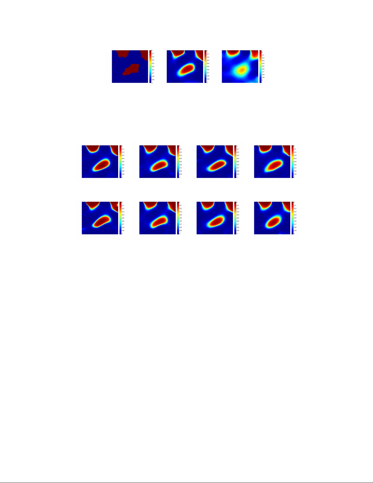
Assessing sto c hastic algorithms for large scale nonlinear least squares problems using extremal probabilities of linear com binations of gamma random v ariables F arb od Ro osta-Khorasani ∗ G´ ab or J. Sz ´ ek ely † Uri M. Asc her ∗ Octob er 20, 2018 Abstract This article considers sto c hastic algorithms for efficien tly solving a class of large scale non-linear least squares (NLS) problems whic h frequen tly arise in ap- plications. W e prop ose eigh t v ariants of a practical randomized algorithm where the uncertain ties in the ma jor sto c hastic steps are quan tified. Suc h sto c has- tic steps in volv e appro ximating the NLS ob jective function using Mon te-Carlo metho ds, and this is equiv alen t to the estimation of the trace of corresp onding symmetric p ositive semi-definite (SPSD) matrices. F or the latter, we prov e tight ne c essary and sufficient conditions on the sample size (which translates to cost) to satisfy the prescrib ed probabilistic accuracy . W e sho w that these conditions are practically computable and yield small sample sizes. They are then incorp orated in our sto c hastic algorithm to quan tify the uncertaint y in eac h randomized step. The b ounds we use are applications of more general results regarding extremal tail probabilities of linear com binations of gamma distributed random v ariables. W e deriv e and prov e new results concerning the maximal and minimal tail probabilities of suc h linear com binations, whic h can b e considered indep endently of the rest of this pap er. 1 In tro duction Large scale data fitting problems arise often in man y applications in science and engineering. As the ability to gather larger amounts of data increases, the need to ∗ Dept. of Computer Science, Univ ersit y of British Columbia, V ancouver, Canada. farbod/ascher@cs.ubc.ca . The work of these authors w as partially funded by NSERC gran t 84306. † National Science F oundation, Arlington, Virginia. gszekely@nsf.gov and Alfr´ ed R ´ en yi Insti- tute of Mathematics, Hungarian Academy of Sciences, Budapest, Hungary . 1 2 devise algorithms to efficien tly solve such problems b ecomes more imp ortan t. The main ob jectiv e here is typically to reco v er some mo del parameters, and it is a widely accepted w orking assumpt ion that having more data can only help (at w orst not h urt) the mo del reco very . Consider the system 1 d i = f i ( m ) + η i , i = 1 , 2 , . . . , s, (1) where d i ∈ R l is the measurement data obtained in the i th exp erimen t, f i = f i ( m ) is the kno wn forw ard op erator (or data predictor) for the i th exp erimen t, m ∈ R l m is the sough t-after parameter vector 2 , and η i is the noise incurred in the i th exp erimen t. The total n umber of exp eriments, or data sets, is assumed large: s  1. The goal is to find (or infer) the unkno wn mo del, m , from the measurements d i , i = 1 , 2 , . . . , s . Gener- ally , this problem can b e ill-p osed. V arious approac hes, including differen t regulariza- tion techniques, ha ve b een prop osed to alleviate this ill-p osedness; see, e.g., [ 33 , 13 ]. In this pap er we assume that the forw ard op erators hav e the form f i ( m ) = f ( m , q i ) , i = 1 , . . . , s, (2) where q i are inputs such that the i th data set, d i , is measured after injecting the i th input (or source) q i in to the system. Th us, for an input q i , f ( m , q i ) predicts the i th measuremen t, giv en the underlying mo del m . W e only consider a sp ecial case where q i ∈ R l q , ∀ i , and f is linear in q , i.e., f ( m , w 1 q 1 + w 2 q 2 ) = w 1 f ( m , q 1 ) + w 2 f ( m , q 2 ). Alternativ ely , w e write f ( m , q ) = G ( m ) q , where G ∈ R l × l q is a matrix that dep ends non-linearly on the sough t m . W e also assume that the task of ev aluating f for each input, q i , is computationally exp ensive. Examples of such a situation arise frequen tly in PDE constrained in verse problems with many data sets; see, e.g., [ 18 , 10 , 30 ] and references therein. Under the further assumption that the indep enden t noise satisfies 3 η i ∼ N (0 , σ I ) , ∀ i , where N denotes normal distribution, I ∈ R l × l denotes the iden tity matrix and σ > 0, the standard maximum likeliho o d (ML) approach leads to mini- mizing the ` 2 misfit function φ ( m ) : = s X i =1 k f ( m , q i ) − d i k 2 2 . (3) Ho wev er, since the ab o v e in verse problem is typically ill-p osed, a regularization func- tional, R ( m ), is often added to the ab o ve ob jective, th us minimizing instead φ R,α ( m ) : = φ ( m ) + αR ( m ) , (4) 1 In this paper, w e use b old low er case to denote vectors and regular capital letters to denote matrices. 2 The parameter vector m often arises from a parameter function in several space v ariables pro jected onto a discrete grid and reshap ed in to a v ector. 3 F or notational simplicity , we do not distinguish b etw een a random vector (e.g., noise) and its realization, as they are clear within the context in which they are used. 3 where α is a regularization parameter [ 13 ]. In general, this regularization term can b e chosen using a priori knowledge of the desired mo del. The ob jective functional ( 4 ) coincides with the maximum a p osteriori (MAP) form ulation. Implicit regularization also exists in which there is no explicit term R ( m ) in the ob jective [ 20 , 10 ]. V arious optimization tec hniques can be used to decrease the v alue of the ab ov e ob jective functionals, ( 3 ) or ( 4 ), to a desired level (determined, e.g., by a given tolerance which dep ends on the noise level), th us reco vering the sought-after mo del. Algorithms that rely on efficien tly approximating the misfit function φ ( m ) hav e b een proposed and studied in [ 18 , 10 , 30 , 29 , 28 ]. In effect, they dra w upon estimating the trace of an implicit 4 symmetric p ositive semi-definite (SPSD) matrix. T o see this, rewrite ( 3 ) as φ ( m ) = k F ( m ) − D k 2 F , (5) where F ( m ) and D are l × s matrices whose i th columns are, respectively , f ( m , q i ) and d i , and k · k F stands for the F rob enius norm. Now, letting B = B ( m ) : = F ( m ) − D , it can b e shown that φ ( m ) = k B k 2 F = tr ( B T B ) = E ( k B w k 2 2 ) , (6) where w is a random v ector drawn from any distribution satisfying E ( ww T ) = I , tr ( A ) denotes the trace of the matrix A , and E denotes the exp ectation. Hence, ap- pro ximating the misfit function φ ( m ) in ( 3 ) or in ( 4 ) is equiv alent to approximating the corresp onding matrix trace (or equiv alen tly , approximating the ab o ve exp ecta- tion). The standard approac h for doing this is based on a Mon te-Carlo metho d, where one generates n random vector realizations, w j , from a suitable probabilit y distribution and computes the empirical mean b φ ( m , n ) : = 1 n n X j =1 k B ( m ) w j k 2 2 ≈ φ ( m ) . (7) Note that b φ ( m , n ) is an unbiase d estimator of φ ( m ), as w e hav e φ ( m ) = E ( b φ ( m , n )). F or the special case of the forward op erators ( 2 ) considered in this pap er, if n  s then this pro cedure yields a very efficient algorithm for approximating the misfit ( 3 ), b ecause s X i =1 f ( m , q i ) w i = f ( m , s X i =1 q i w i ) , whic h can b e computed with a single ev aluation of f p er realization of the random v ector w = ( w 1 , . . . , w s ) T . Our assumption regarding the noise distribution leading to the ordinary least squares misfit function ( 3 ), although standard, is quite simplistic. F ortunately , how- ev er, it can b e readily generalized in one of the following t wo w ays. 4 By “implicit matrix” we mean that the matrix of in terest is not a v ailable explicitly: only infor- mation in the form of matrix-vector pro ducts for any appropriate v ector is av ailable. 4 1. The noise is indep endent and identically distributed (i.i.d) as η i ∼ N (0 , Σ) , ∀ i , where Σ ∈ R l × l is the symmetric p ositive definite cov ariance matrix. In this case, the ML approac h leads to minimizing the ` 2 misfit function φ (1) ( m ) : = s X i =1 k C − 1  f ( m , q i ) − d i  k 2 2 , (8) where C ∈ R l × l is any inv ertible matrix such that Σ = C C T (e.g., C can b e the Cholesky factor of Σ). Thus, φ (1) ( m ) = k C − 1  F ( m ) − D  k 2 F = k B ( m ) k 2 F , with B ( m ) : = C − 1  F ( m ) − D  . The Mon te-Carlo appro ximation b φ (1) ( m , n ) is then precisely as in ( 7 ) but with the newly defined B ( m ). 2. The noise is independen t but not iden tically distributed, satisfying instead η i ∼ N (0 , σ 2 i I ) , i = 1 , 2 , . . . , s , where σ i > 0 are the standard deviations. Under this assumption, the ML approac h yields the weighte d le ast squar es misfit function φ (2) ( m ) : = s X i =1 1 σ 2 i k f ( m , q i ) − d i k 2 2 . (9) W e can further write this equation as φ (2) ( m ) = k  F ( m ) − D  C − 1 k 2 F , where C ∈ R s × s denotes the diagonal matrix whose i th diagonal element is σ i . Th us, with B ( m ) = ( F ( m ) − D ) C − 1 w e can again apply ( 7 ) to obtain a similar Mon te-Carlo appro ximation b φ (2) ( m , n ). No w, if n  s then the unbiased estimators b φ (1) ( m , n ) and b φ (2) ( m , n ) are obtained with a similar efficiency as b φ ( m , n ). In the sequel, for notational simplicity , w e just concen trate on φ ( m ) and b φ ( m , n ), but all the results hold almost v erbatim also for ( 8 ) and ( 9 ). Hence, the ob jectiv e is to b e able to generate as few realizations of w as p ossible for ac hieving acceptable approximations to the misfit function. Estimates on how large n must b e to ac hieve a prescribed accuracy in a probabilistic sense hav e b een deriv ed in [ 1 , 3 , 34 , 28 ]. How ev er, the obtained b ounds are t ypically not sufficiently tigh t to b e practically useful. In the presen t pap er, we pro v e tight b ounds for tail probabilities for such Mon te-Carlo approximations emplo ying the standard normal distribution. These tail b ounds are then used to obtain ne c essary and sufficient b ounds on n , and we demonstrate that these b ounds can b e practically small and computable. F urthermore, using these results, w e are able to b etter quantify the 5 uncertain ties in the highly efficien t randomized algorithms prop osed in [ 10 , 30 , 29 ]. V ariants of suc h algorithms with b etter uncertaint y quan tification are derived. This paper is organized as follo ws. In Section 2 , w e dev elop and state theorems regarding the tigh t tail bounds promised abov e. The theory in this section relies upon some no vel results regarding the extremal probabilities (i.e., maxima and minima of the tail probabilities) of non-negative linear combinations of gamma random v ariables, whic h are prov ed in App endix B . In Section 3 we presen t our sto chastic algorithm v ariants for approximately min- imizing ( 3 ) or ( 4 ) and discuss its no v el elemen ts. Subsequently in Section 4 , the efficiency of the prop osed algorithm v ariants is demonstrated using an important class of problems that arise often in practice. This is follow ed by conclusions and further thoughts in Section 5 . 2 Matrix trace estimation Let the matrix A = B T B ∈ R s × s b e implicit SPSD, and denote its trace b y tr ( A ). As describ ed in Section 1 , w e appro ximate tr ( A ) by tr n ( A ) : = 1 n n X j =1 w T j A w j , (10) where w j ∈ R s ∼ N (0 , I ). No w, given a pair of small p ositiv e real num b ers ( ε, δ ), consider finding an appro- priate sample size n such that Pr  tr n ( A ) ≥ (1 − ε ) tr ( A )  ≥ 1 − δ, (11a) Pr  tr n ( A ) ≤ (1 + ε ) tr ( A )  ≥ 1 − δ. (11b) In [ 28 ] we sho wed that the inequalities ( 11 ) hold if n > 8 c, where c = c ( ε, δ ) = ε − 2 ln(1 /δ ) . (12) Ho wev er, this b ound on n can b e rather p essimistic. Theorems 3 and 4 and Corollary 5 b elo w provide tigh ter and hop efully more useful b ounds on n . In order to pro v e these w e require the tw o additional Theorems 1 and 2 , whose nontrivial and more tec hnical pro ofs are deferred to App endix B . Let X ∼ Gamma ( α, β ) denote a gamma distributed random v ariable (r.v) parametrized by shape α and rate β 5 . 5 Recall that the probabilit y density function of such r.v is f ( x ) = ( β α Γ( α ) x α − 1 e − β x x ≥ 0 , 0 x < 0 . 6 Theorem 1 (Monotonicit y of cum ulativ e distribution function of gamma r.v ) Given p ar ameters 0 < α 1 < α 2 , let X i ∼ Gamma ( α i , α i ) , i = 1 , 2 , b e indep endent r.v’s, and define ∆( x ) : = Pr( X 2 < x ) − Pr( X 1 < x ) . Then we have that (i) ther e is a unique p oint x ( α 1 , α 2 ) such that ∆( x ) < 0 for 0 < x < x ( α 1 , α 2 ) and ∆( x ) > 0 for x > x ( α 1 , α 2 ) , (ii) 1 ≤ x ( α 1 , α 2 ) ≤ 2 √ α 1 ( α 2 − α 1 )+1 2 √ α 1 ( α 2 − α 1 ) . Theorem 2 (Extremal probabilities of linear com bination of gamma r.v’s) Given shap e and r ate p ar ameters α, β > 0 , let X i ∼ Gamma ( α, β ) , i = 1 , 2 , . . . , n , b e i.i.d gamma r.v’s, and define Θ : = { λ =  λ 1 , λ 2 , . . . , λ n  T | λ i ≥ 0 ∀ i, n X i =1 λ i = 1 } . Then we have m n ( x ) : = min λ ∈ Θ Pr n X i =1 λ i X i < x ! =    Pr  1 n P n i =1 X i < x  , x < α β Pr  X 1 < x  , x > 2 α +1 2 β , M n ( x ) : = max λ ∈ Θ Pr n X i =1 λ i X i < x ! =    Pr  X 1 < x  , x < α β Pr  1 n P n i =1 X i < x  , x > 2 α +1 2 β . Next w e state and prov e the results that are directly relev ant to this section. Let us define Q ( n ) : = 1 n Q n , where Q n ∼ χ 2 n denotes a chi-squared r.v of degree n . Note that Q ( n ) ∼ Gamma ( n/ 2 , n/ 2). In case of several i.i.d gamma r.v’s of this sort, we refer to the j th r.v by Q j ( n ). Theorem 3 (Necessary and sufficient condition for ( 11a ) ) Given an SPSD matrix A of r ank r and toler anc es ( ε, δ ) as ab ove, the fol lowing hold: 7 (i) Sufficient c ondition: ther e exists some inte ger n 0 ≥ 1 such that Pr  Q ( n 0 ) < (1 − ε )  ≤ δ. (13) F urthermor e, ( 11a ) holds for al l n ≥ n 0 . (ii) Ne c essary c ondition: if ( 11a ) holds for some n 0 ≥ 1 , then for al l n ≥ n 0 P − ε,r ( n ) : = Pr  Q ( nr ) < (1 − ε )  ≤ δ. (14) (iii) Tightness: if the r p ositive eigenvalues of A ar e al l e qual (NB this always hap- p ens if r = 1 ), then ther e is a p ositive inte ger n 0 satisfying ( 14 ) , such that ( 11a ) holds iff n ≥ n 0 . Pro of Since A is SPSD, it can be diagonalized b y a unitary similarit y transformation as A = U T Λ U , where Λ is the diagonal matrix of eigenv alues sorted in non-increasing order. Consider n random v ectors w i , i = 1 , . . . , n , whose comp onen ts are i.i.d and dra wn from the standard normal distribution, and define z i = U w i for eac h i . Note that since U is unitary , the en tries of z i are i.i.d standard normal v ariables, lik e the en tries of w i . W e ha ve tr n ( A ) tr ( A ) = 1 n tr ( A ) n X i =1 w T i A w i = 1 n tr ( A ) n X i =1 z T i Λ z i = 1 n tr ( A ) n X i =1 r X j =1 λ j z 2 ij = r X j =1 λ j n tr ( A ) n X i =1 z 2 ij = r X j =1 λ j tr ( A ) Q j ( n ) , where the λ j ’s appearing in the sums are p ositive eigen v alues of A. Now, noting that P r j =1 λ j tr ( A ) = 1, Theorem 2 yields Pr r X j =1 λ j tr ( A ) Q j ( n ) ≤ (1 − ε ) ! ≤ Pr  Q ( n ) ≤ (1 − ε )  = P − ε, 1 ( n ) , (15a) Pr r X j =1 λ j tr ( A ) Q j ( n ) ≤ (1 − ε ) ! ≥ Pr  Q ( nr ) ≤ (1 − ε )  = P − ε,r ( n ) . (15b) In addition, for an y given r > 0 and ε > 0, the function P − ε,r ( n ) is monotonically decreasing on integers n ≥ 1. This can b e seen b y Theorem 1 using the sequence α i = ( n 0 + ( i − 1)) r / 2 , i ≥ 1. The claims no w easily follo w b y com bining ( 15 ) and this decreasing prop ert y .  Theorem 4 (Necessary and sufficient condition for ( 11b ) ) Given an SPSD matrix A of r ank r and toler anc es ( ε, δ ) as ab ove, the fol lowing hold: 8 (i) Sufficient c ondition: if the ine quality Pr  Q ( n 0 ) ≤ (1 + ε )  ≥ 1 − δ (16) is satisfie d for some n 0 > ε − 1 , then ( 11b ) holds with n = n 0 . F urthermor e, ther e is always an n 0 > ε − 2 such that ( 16 ) is satisfie d and, for such n 0 , it fol lows that ( 11b ) holds for al l n ≥ n 0 . (ii) Ne c essary c ondition: if ( 11b ) holds for some n 0 > ε − 1 , then P + ε,r ( n ) : = Pr  Q ( nr ) ≤ (1 + ε )  ≥ 1 − δ , (17) with n = n 0 . F urthermor e, if n 0 > ε − 2 r − 2 , then ( 17 ) holds for al l n ≥ n 0 . (iii) Tightness: if the r p ositive eigenvalues of A ar e al l e qual, then ther e is a smal lest n 0 > ε − 2 r − 2 satisfying ( 17 ) such that for any n ≥ n 0 , ( 11b ) holds, and for any ε 2 r − 2 < n < n 0 , ( 11b ) do es not hold. If δ is smal l enough so that ( 17 ) do es not hold for any n ≤ ε 2 r − 2 , then n 0 is b oth ne c essary and sufficient for ( 11b ) . Pro of The same unitary diagonalization argumen t as in the proof of Theorem 3 sho ws that Pr  tr n ( A ) < (1 + ε ) tr ( A )  = Pr r X j =1 λ j tr ( A ) Q j ( n ) < (1 + ε ) ! . No w w e see that if n > ε − 1 , Theorem 2 with α = n/ 2 yields Pr r X j =1 λ j tr ( A ) Q j ( n ) ≤ (1 + ε ) ! ≥ Pr  Q ( n ) ≤ (1 + ε )  = P + ε, 1 ( n ) , (18a) Pr r X j =1 λ j tr ( A ) Q j ( n ) ≤ (1 + ε ) ! ≤ Pr  Q ( nr ) ≤ (1 + ε )  = P + ε,r ( n ) . (18b) In addition, for an y given r > 0 and ε > 0, the function P + ε,r ( n ) is monotonically increasing on in tegers n > ε − 2 r − 2 . This can b e seen by Theorem 1 using the sequence α i = ( n 0 + ( i − 1)) r / 2 , i ≥ 1. The claims no w easily follo w b y com bining ( 18 ) and this increasing prop ert y .  Remarks: (i) P art (iii) of Theorem 4 states that if δ is not small enough, then n 0 migh t not b e a necessary and sufficient sample size for the sp ecial matrices men tioned there, i.e., matrices with λ 1 = λ 2 = · · · = λ r . This can b e seen from Figure 1 (b): for r = 1 , ε = 0 . 1, if δ = 0 . 33, say , there is an integer 10 < n ≤ 100 such that ( 11b ) holds, so n = 101 is no longer a necessary sample size (although it is still sufficient). 9 (a) (b) Figure 1: The curves of P − ε,r ( n ) and P + ε,r ( n ), defined in ( 14 ) and ( 17 ), for ε = 0 . 1 and r = 1: (a) P − ε,r ( n ) decreases monotonically for all n ≥ 1; (b) P + ε,r ( n ) increases monotonically only for n ≥ n 0 , where n 0 > 1: according to Theorem 4 , n 0 = 100 is safe, and this v alue do es not disagree with the plot. (ii) Sim ulations sho w that the sufficien t sample size obtained using Theorems 3 and 4 , amoun ts to b ounds of the form O ( c ( ε, δ ) g ( δ )), where g ( δ ) < 1 is a decreasing function of δ and c ( ε, δ ) is as defined in ( 12 ). As suc h, for larger v alues of δ , i.e., when larger uncertaint y is allow ed, one can obtain significantly smaller sample sizes than the one predicted b y ( 12 ); see Figures 2 and 3 . In other w ords, the difference b et ween the ab o ve tighter conditions and ( 12 ) is increasingly more prominent as δ gets larger. (iii) Note that the results in Theorems 3 and 4 are indep endent of the size of the matrix. In fact, the first items (i) in b oth theorems do not require an y a priori kno wledge ab out the matrix, other than it b eing SPSD. In order to compute the necessary sample sizes, though, one is required to also know the rank of the matrix. (iv) The conditions in our theorems, despite their p otentially ominous lo ok, are actually simple to compute. App endix C contains a short Ma tlab co de whic h calculates these necessary or sufficient sample sizes to satisfy the probabilistic accuracy guarantees ( 11 ), giv en a pair ( ε, δ ) (and the matrix rank r in case of necessary sample sizes). This co de was used for generating Figures 2 and 3 . Com bining Theorems 3 and 4 , w e can easily state conditions on the sample size n for which the condition Pr  | tr n ( A ) − tr ( A ) | ≤ ε tr ( A )  ≥ 1 − δ (19) holds. W e ha ve the following immediate corollary: 10 (a) (b) Figure 2: Comparing, as a function of δ , the sample size obtained from ( 13 ) and denoted by “tight”, with that of ( 12 ) and denoted by “lo ose”, for ε = 0 . 1 and 0 . 01 ≤ δ ≤ 0 . 3: (a) sufficient sample size, n , for ( 11a ), (b) ratio of sufficient sample size obtained from ( 12 ) o v er that of ( 13 ). When δ is relaxed, our new b ound is tighter than the older one by an order of magnitude. Corollary 5 (Necessary and sufficient condition for ( 19 ) ) Given an SPSD matrix A of r ank r and toler anc es ( ε, δ ) as ab ove, the fol lowing hold: (i) Sufficient c ondition: if the ine quality Pr  (1 − ε ) ≤ Q ( n 0 ) ≤ (1 + ε )  ≥ 1 − δ (20) is satisfie d for some n 0 > ε − 1 , then ( 19 ) holds with n = n 0 . F urthermor e, ther e is always an n 0 > ε − 2 such that ( 20 ) is satisfie d and, for such n 0 , it fol lows that ( 19 ) holds for al l n ≥ n 0 . (ii) Ne c essary c ondition: if ( 19 ) holds for some n 0 > ε − 1 , then Pr  (1 − ε ) ≤ Q ( nr ) ≤ (1 + ε )  ≥ 1 − δ , (21) with n = n 0 . F urthermor e, if n 0 > ε − 2 r − 2 , then ( 21 ) holds for al l n ≥ n 0 . (iii) Tightness: if the r p ositive eigenvalues of A ar e al l e qual then ther e is a smal lest n 0 > ε − 2 r − 2 satisfying ( 21 ) such that for any n ≥ n 0 , ( 19 ) holds, and for any ε − 2 r − 2 < n < n 0 , ( 19 ) do es not hold. If δ is smal l enough so that ( 21 ) do es not hold for any n ≤ ε − 2 r − 2 , then n 0 is b oth ne c essary and sufficient for ( 19 ) . Remark: The necessary condition in Corollary 5 (ii) is only v alid for n > ε − 1 (this is a consequence of the condition ( 21 ) b eing tight, as sho wn in part (iii)). In [ 28 ], an “almost tight” necessary condition is given that works for all n ≥ 1. 11 (a) (b) Figure 3: Comparing, as a function of δ , the sample size obtained from ( 16 ) and denoted by “tight”, with that of ( 12 ) and denoted by “lo ose”, for ε = 0 . 1 and 0 . 01 ≤ δ ≤ 0 . 3: (a) sufficient sample size, n , for ( 11b ), (b) ratio of sufficien t sample size obtained from ( 12 ) o v er that of ( 16 ). When δ is relaxed, our new b ound is tighter than the older one by an order of magnitude. 3 Randomized algorithms for solving large scale NLS problems Consider the problem of decreasing the v alue of the original ob jectiv e ( 3 ) to a desired lev el (e.g., satisfying a giv en tolerance) to recov er the sought mo del, m . With the sensitivit y matrices J i ( m ) = ∂ f ( m , q i ) ∂ m , i = 1 , . . . , s w e ha ve the gradient ∇ φ ( m ) = 2 s X i =1 J T i ( m )( f ( m , q i ) − d i ) . An iterative method suc h as mo dified Gauss-Newton (GN), L-BFGS, or nonlinear conjugate gradien t is t ypically designed to decrease the v alue of the ob jectiv e function using rep eated calculations of the gradien t. In the presen t article we follow [ 30 ] and emplo y v ariants of stabilized GN throughout, th us ac hieving a con text in which to fo cus our atten tion on the new asp ects of this work. In the k th iteration of such a metho d, having the curren t iterate m k , an up date direction, δ m k , is calculated. Then the iterate is updated as m k +1 ← m k + α k δ m k , for some appropriate step length α k . What is special in our con text here is that the update direction, δ m k , is calculated using the approximate misfit, b φ ( m k , n k ), defined as describ ed in ( 7 ) ( n k is the sample 12 size used for this appro ximation in the k th iteration). Thus, w e need to c heck or assess whether the v alue of the original ob jective is also decreased using this new iterate. The c hallenge is to do this as w ell as c heck for termination of the iteration pro cess with a minimal num b er of ev aluations of the prohibitively expensive original misfit function φ . In this section, w e extend the algorithms introduced in [ 30 , 29 ] in the context of the more general NLS form ulation ( 8 ) or ( 9 ), assuming that their corresp onding noise distributions hold, although, as promised in Section 1 , we stic k to the simpler notation ( 3 ), ( 7 ). V ariants of mo dified sto chastic steps in the original algorithms are presen ted, and using Theorems 3 and 4 , the uncertainties in these steps are quan tified. More sp ecifically , in the main algorithm introduced in [ 30 ], following a stabilized GN iteration on the approximated ob jective function using the approximated misfit, the iterate is up dated, and some (or all) of the following steps are p erformed: (i) cr oss validation – appro ximate assessment of this iterate in terms of sufficien t decrease in the ob jective function using a con trol set of random combinations of measurements. More sp ecifically , at the k th iteration with the new iterate m k +1 , we test whether the condition b φ ( m k +1 , n k ) ≤ κ b φ ( m k , n k ) (22) (cf. ( 7 )) holds for some κ ≤ 1, employing an indep endent set of weigh t vectors used in b oth approximations of φ ; (ii) unc ertainty che ck – up on success of cross v alidation, an inexp ensive plausible termination test is p erformed where, given a tolerance ρ , w e chec k for the con- dition b φ ( m k +1 , n k ) ≤ ρ (23) using a fresh set of random w eigh t v ectors; and (iii) stopping criterion – up on success of the uncertaint y chec k, an additional inde- p enden t and p oten tially more rigorous termination test against the giv en toler- ance ρ is p erformed (p ossibly using the original misfit function). The role of the cross v alidation step within an iteration is to assess whether the true ob jectiv e function at the curren t iterate has (sufficiently) decreased compared to the previous one. If this test fails, we deem that the curren t sample size is not sufficien tly large to yield an update that decreases the original ob jectiv e, and the fitting step needs to b e rep eated using a larger sample size, see [ 10 ]. In [ 30 ], this step w as used heuristically , so the amount of uncertain ty in suc h v alidation of the curren t iterate was not quantified. Consequen tly , there w as no handle on the amount of false positives/negativ es in such approximate ev aluations (e.g., a sample size could b e deemed to o small while the stabilized GN iteration has in fact pro duced an ac- ceptable iterate). In addition, in [ 30 ] the sample size for the uncertaint y c heck was 13 heuristically c hosen. So this step was also performed with no control o ver the amoun t of uncertaint y . F or the stopping criterion step in [ 30 , 10 ], the ob jective function w as accurately ev aluated using all s exp eriments, whic h is clearly a v ery exp ensiv e c hoice for an algorithm termination chec k. This w as a judicious decision made in order to b e able to hav e a fairer comparison of the new and different metho ds prop osed there. Re- placemen t of this termination criterion by another independent heuristic “uncertain ty c heck” is exp erimented with in [ 29 ]. In this section, we address the issues of quan tifying the uncertaint y in the v alida- tion, uncertaint y chec k and stopping criterion steps within a nonlinear iteration. In what follo ws, w e assume for simplicity that the iterations are p erformed on the ob- jectiv e ( 3 ) using dynamic regularization (or iterative regularization [ 20 , 9 , 10 ]) where the regularization is performed implicitly . Extension to the case ( 4 ) is straigh t for- w ard. Throughout, w e assume to b e given a pair of p ositive and small probabilistic tolerance num b ers, ( ε, δ ). 3.1 Cross v alidation step with quan tified uncertain t y The condition ( 22 ) is an indep enden t, un biased indicator of φ ( m k +1 ) ≤ κφ ( m k ) , whic h indicates sufficien t decrease in the ob jectiv e. If ( 22 ) is satisfied then the cur- ren t sample size, n k , is considered sufficiently large to capture the original misfit well enough to pro duce a v alid iterate, and the algorithm contin ues using the same sample size. Otherwise, the sample size is deemed insufficient and is increased. Using Theo- rems 3 and 4 , w e can no w remov e the heuristic characteristic as to when this sample size increase has b een p erformed hitherto, and present t wo v ariants of ( 22 ) where the uncertain ties in the v alidation step are quantified. Assume we ha ve a sample size n c suc h that P r  b φ ( m k , n c ) ≤ (1 + ε ) φ ( m k )  ≥ 1 − δ, (24a) P r  b φ ( m k +1 , n c ) ≥ (1 − ε ) φ ( m k +1 )  ≥ 1 − δ. (24b) If in the pro cedure outlined ab ov e, after obtaining the up dated iterate m k +1 , w e v erify that b φ ( m k +1 , n c ) ≤ κ  1 − ε 1 + ε  b φ ( m k , n c ) , (25) then it follo ws from ( 24 ) that φ ( m k +1 ) ≤ κφ ( m k ) with a probabilit y of, at least, (1 − δ ) 2 . In other words, success of ( 25 ) indicates that the up dated iterate decreases the v alue of the original misfit ( 3 ) with a probability of, at least, (1 − δ ) 2 . 14 Alternativ ely , supp ose that we ha ve P r  b φ ( m k , n c ) ≥ (1 − ε ) φ ( m k )  ≥ 1 − δ, (26a) P r  b φ ( m k +1 , n c ) ≤ (1 + ε ) φ ( m k +1 )  ≥ 1 − δ. (26b) No w, if instead of ( 25 ) we c heck whether or not b φ ( m k +1 , n c ) ≤ κ  1 + ε 1 − ε  b φ ( m k , n c ) , (27) then it follows from ( 26 ) that if the condition ( 27 ) is not satisfied, then φ ( m k +1 ) > κφ ( m k ) with a probability of, at least, (1 − δ ) 2 . In other w ords, failure of ( 27 ) indicates that the updated iterate results in an insufficien t decrease in the original misfit ( 3 ) with a probability of, at least, (1 − δ ) 2 . W e can replace ( 22 ) with either of the conditions ( 25 ) or ( 27 ) and use the con- ditions ( 13 ) or ( 16 ) to calculate the cross v alidation sample size, n c . If the relev ant c heck ( 25 ) or ( 27 ) fails, we deem the sample size used in the fitting step, n k , to b e to o small to pro duce an iterate which decreases the original misfit ( 3 ), and consequen tly consider increasing the sample size, n k . Note that since 1 − ε 1+ ε < 1 < 1+ ε 1 − ε , the con- dition ( 25 ) results in a more aggressive strategy for increasing the sample size used in the fitting step than the condition ( 27 ). Figure 8 in Section 4 demonstrates this within the context of an application. Remarks: (i) Larger v alues of ε result in more aggressiv e (or relaxed) descent requirement by the condition ( 25 ) (or ( 27 )). (ii) As the iterations progress and w e get closer to the solution, the decrease in the original ob jectiv e could b e less than what is imp osed by ( 25 ). As a result, if ε is to o large, we might nev er successfully pass the cross v alidation test. One useful strategy to alleviate this is to start with a larger ε , decreasing it as w e get closer to the solution. A similar strategy can b e adopted for the case when the condition ( 27 ) is used as a cross v alidation: as the iterations get closer to the solution, one can make the condition ( 27 ) less relaxed by decreasing ε . 3.2 Uncertain t y c hec k with quan tified uncertain t y and effi- cien t stopping criterion The usual test for terminating the iterativ e pro cess is to chec k whether φ ( m k +1 ) ≤ ρ, (28) for a giv en tolerance ρ . Ho w ever, this can b e very exp ensive in ou r current context; see Section 4.1 and T ables 1 and 2 for examples of a scenario where one misfit ev aluation 15 using the en tire data set can b e as expensive as the en tire cost of an efficien t, complete algorithm. In addition, if the exact v alue of the tolerance ρ is not known (which is usually the case in practice), one should b e able to reflect suc h uncertain ty in the stopping criterion and p erform a softer version of ( 28 ). Hence, it could be useful to ha ve an algorithm which allows one to adjust the cost and accuracy of such an ev aluation in a quantifiable w ay , and find the balance that is suitable to particular ob jectives and computational resources. Regardless of the issues of cost and accuracy , this ev aluation should b e carried out as rarely as p ossible and only when deemed timely . In [ 30 ], w e addressed this b y employing an “uncertaint y c heck” ( 23 ) as describ ed earlier in this section, heuris- tically . Using Theorems 3 and 4 , w e no w devise v ariants of ( 23 ) with quantifiable uncertain ty . Subsequently , again using Theorems 3 and 4 , we presen t a muc h cheaper stopping criterion than ( 28 ) whic h, at the same time, reflects our uncertaint y in the giv en tolerance. Assume that we ha ve a sample size n u suc h that P r  b φ ( m k +1 , n u ) ≥ (1 − ε ) φ ( m k +1 )  ≥ 1 − δ . (29) If the up dated iterate, m k +1 , successfully passes the cross v alidation test, then we c heck for b φ ( m k +1 , n u ) ≤ (1 − ε ) ρ. (30) If this holds to o then it follows from ( 29 ) that φ ( m k +1 ) ≤ ρ with a probability of, at least, (1 − δ ). In other words, success of ( 30 ) indicates that the misfit is likely to b e b elo w the tolerance with a probability of, at least, (1 − δ ). Alternativ ely , supp ose that P r  b φ ( m k +1 , n u ) ≤ (1 + ε ) φ ( m k +1 )  ≥ 1 − δ , (31) and instead of ( 30 ) we c heck for b φ ( m k +1 , n u ) ≤ (1 + ε ) ρ. (32) then it follo ws from ( 31 ) that if the condition ( 32 ) is not satisfied, then φ ( m k +1 ) > ρ with a probabilit y of, at least, (1 − δ ). In other w ords, failure of ( 32 ) indicates that using the up dated iterate, the misfit is lik ely to be still ab o v e the desired tolerance with a probability of, at least, (1 − δ ). W e can replace ( 23 ) with the condition ( 30 ) (or ( 32 )) and use the condition ( 13 ) (or ( 16 )) to calculate the uncertaint y c heck sample size, n u . If the test ( 30 ) (or ( 32 )) fails then we skip the stopping criterion chec k and contin ue iterating. Note that since (1 − ε ) < 1 < (1 + ε ), the condition ( 30 ) results in few er false p ositives than the condition ( 32 ). On the other hand, the condition ( 32 ) is exp ected to results in few er false negativ es than the condition ( 30 ). The c hoice of either alternative is dep endent on one’s requirements, resources and the application on hand. 16 The stopping criterion step can b e p erformed in the same w ay as the uncertaint y c heck but p otentially with higher certaint y in the outcome. In other words, for the stopping criterion w e can c ho ose a smaller δ , resulting in a larger sample size n t satisfying n t > n u , and chec k for satisfaction of either b φ ( m k +1 , n t ) ≤ (1 − ε ) ρ, (33a) or b φ ( m k +1 , n t ) ≤ (1 + ε ) ρ. (33b) Clearly the condition ( 33b ) is a softer than ( 33a ): a successful ( 33b ) is o nly necessary and not sufficient for concluding that ( 28 ) holds with the prescrib ed probabilit y . In practice, when the v alue of the stopping criterion threshold, ρ , is not exactly kno wn (it is often crudely estimated using the measuremen ts), one can reflect suc h uncertain ty in ρ b y c ho osing an appropriately large δ . Smaller v alues of δ reflect a higher certaint y in ρ and a more rigid stopping criterion. Remarks: (i) If ε is large then using ( 33a ), one migh t run the risk of ov er-fitting. Similarly , using ( 33b ) with large ε , there is a risk of under-fitting. Thus, appropriate v alues of ε need to b e considered in accordance with the application and one’s computational resources and exp erience. (ii) The same issues regarding large ε arise when emplo ying the uncertaint y c heck condition ( 30 ) (or ( 32 )): large ε might increase the frequency of false negativ es (or p ositives). 3.3 Algorithm W e now present an efficien t, sto c hastic, iterative algorithm for approximately solving NLS form ulations of ( 3 ) or ( 4 ). By p erforming cross v alidation, uncertaint y chec k and stopping criterion as descried in Section 3.1 and Section 3.2 , w e can devise 8 v ariants of Algorithm 1 below. Dep ending on the application, the v ariant of choice can b e selected appropriately . More sp ecifically , cross v alidation, uncertain ty chec k and stopping criterion can, respectively , b e c hosen to b e one of the follo wing com binations (referring to their equation num b ers): (i) ( 25 - 30 - 33a ) (ii) ( 25 - 30 - 33b ) (iii) ( 25 - 32 - 33a ) (iv) ( 25 - 32 - 33b ) (v) ( 27 - 30 - 33a ) (vi) ( 27 - 30 - 33b ) (vii) ( 27 - 32 - 33a ) (viii) ( 27 - 32 - 33b ) Remark: 17 (i) The sample size, n k , used in the fitting step of Algorithm 1 could in principle b e determined by Corollary 5 , using a pair of tolerances ( ε f , δ f ). If cross v al- idation ( 25 ) (or ( 27 )) fails, the tolerance pair ( ε f , δ f ) is reduced to obtain, in the next iteration, a larger fitting sample size, n k +1 . This w ould give a sample size whic h yields a quantifiable appro ximation with a desired relative accuracy . Ho wev er, in the presence of all the added safet y steps describ ed in this section, w e hav e found in practice that Algorithm 1 is capable of pro ducing a satisfying reco very , even with a significantly smaller n k than the one predicted by Corol- lary 5 . Thus, the “ how ” of the fitting sample size increase is left to heuristic (as opp osed to its “ when ”, whic h is quantified as describ ed in Section 3.1 ). (ii) In the algorithm b elow, w e only consider fixed v alues (i.e., indep enden t of k ) for ε and δ . One can easily mo dify Algorithm 1 to incorporate non-stationary v alues whic h adapt to the iteration pro cess, as mentioned in the closing remark of Section 3.1 . In Algorithm 1 , when we dra w v ectors w i for some purp ose, we alw ays dra w them indep enden tly from the standard normal distribution. 4 A practical application In this section, w e demonstrate the efficacy of Algorithm 1 by applying it to an imp ortan t class of problems that arise often in practice: large scale partial differen tial equation (PDE) in verse problems with many measuremen ts. W e sho w b elow the capabilit y of our method by applying it to suc h examples in the con text of the DC resistivit y/EIT problem, as in [ 10 , 30 , 29 ]. 4.1 PDE in v erse problems with man y measuremen ts The con text considered here is one where each ev aluation of f i ( m ) in ( 2 ) is compu- tationally exp ensive. The ev aluation of the misfit function φ ( m ) is esp ecially costly when many exp erimen ts, inv olving different com binations of sources and receivers, are employ ed in order to obtain reconstructions of acceptable quality . The sought mo del m is a discretization of the function m ( x ) as describ ed in Section 1 , and f i ( m ) = P i u i = P i L ( m ) − 1 q i . (34a) Here we write the PDE system in discretized form as L ( m ) u i = q i , i = 1 , . . . , s, (34b) where u i ∈ I R l q is the i th field, q i ∈ I R l q is the i th source, and L is a square ma- trix discretizing the PDEs plus appropriate side conditions. F urthermore, the giv en 18 Algorithm 1 Solve NLS form ulation of ( 3 ) (or ( 4 )) using uncertain t y chec k, cross v alidation and c heap stopping criterion Giv en: sources q i , i = 1 , . . . , s , measuremen ts d i , i = 1 , . . . , s , stopping criterion lev el ρ , ob jective function sufficien t decrease factor κ ≤ 1, pairs of small n um b ers ( ε c , δ c ), ( ε u , δ u ), ( ε t , δ t ), and initial guess m 0 . Initialize : - m = m 0 , n 0 = 1 - Calculate the cross v alidation sample size, n c , as describ ed in Section 3.1 with ( ε c , δ c ). - Calculate the sample sizes for uncertain t y c hec k, n u , and stopping criterion, n t , as describ ed in Section 3.2 with ( ε u , δ u ) and ( ε t , δ t ), resp ectively . for k = 0 , 1 , 2 , · · · until termination do Fitting : - Draw w i , i = 1 , . . . , n k . - Approximate the misfit term and p oten tially its gradient in ( 3 ) or ( 4 ) using ( 7 ) with the ab o ve w eights and n = n k . - Find an up date for the ob jective function using the appro ximated misfit ( 7 ). Cross V alidation : - Draw w i , i = 1 , . . . , n c . if ( 25 ) (or ( 27 )) holds then Uncertain ty Check : - Draw w i , i = 1 , . . . , n u . if ( 30 ) (or ( 32 )) holds then Stopping Criterion : - Draw w i , i = 1 , . . . , n t . if ( 33a ) (or ( 33b )) holds then - T erminate end if end if - Set n k +1 = n k . else - Sample Size Increase : for example, set n k +1 = min(2 n k , s ). end if end for 19 pro jection matrices P i are suc h that f i ( m ) predicts the i th data set. Note that the notation ( 34b ) reflects an assumption of linearit y in u but not in m [ 30 ]. If the lo cations where data are measured do not change from one exp eriment to another, i.e., P = P i , ∀ i , then w e get f ( m , q i ) = P L ( m ) − 1 q i , (35) and the linearit y assumption of f ( m , q ) in q is satisfied. Thus, w e can use Algorithm 1 to efficien tly reco v er m and b e quan tifiably confiden t in the recov ered mo del. If the P i ’s are differen t across exp erimen ts, there are metho ds to extend the existing data set to one where all sources share the same receiv ers, see [ 29 , 17 ]. Using these metho ds (when they apply!), one can effectiv ely transform the problem ( 34a ) to ( 35 ), for whic h Algorithm 1 can b e employ ed. There are several problems of practical interest in the form ( 3 ), ( 34 ), where the use of man y exp eriments, resulting in a large num b er s , is crucial for obtaining credible reconstructions in practical situations. These include electromagnetic data inv ersion in mining exploration (e.g., [ 24 , 12 , 16 , 25 ]), seismic data in version in oil exploration (e.g., [ 14 , 21 , 27 ]), diffuse optical tomograph y (DOT) (e.g., [ 2 , 4 ]), quantitativ e photo- acoustic tomograph y (QP A T) (e.g., [ 15 , 35 ]), direct current (DC) resistivit y (e.g., [ 31 , 26 , 19 , 18 , 10 ]), and electrical imp edance tomography (EIT) (e.g., [ 5 , 8 , 11 ]). Our examples are p erformed in the con text of solving the DC resistivit y problem. The PDE has the form ∇ · ( µ ( x ) ∇ u ) = q ( x ) , x ∈ Ω , (36a) where Ω ⊂ I R d , d = 2 or 3, and µ ( x ) is a conductivity function which ma y b e rough 6 (e.g., discontin uous). Ho w ever, the PDE is co ercive: there is a constan t µ 0 > 0 suc h that µ ( x ) ≥ µ 0 , ∀ x ∈ Ω. It is p ossible to inject some a priori information on µ , when suc h is av ailable, via a parametrization of µ ( x ) in terms of m ( x ) using an appropriate transfer function ψ as µ ( x ) = ψ ( m ( x )). F or example, ψ can be c hosen so as to ensure that the conductivit y sta ys p ositiv e and b ounded a wa y from 0, as w ell as to incorp orate b ounds, which are often kno wn in practice, on the sought conductivit y function. Some p ossible c hoices of function ψ are described in [ 30 , App endix A]. Here w e take Ω to b e the unit square in 2D, and assume the homogeneous Neumann b oundary conditions ∂ u ∂ n = 0 , x ∈ ∂ Ω . (36b) The in verse problem is then to reco ver m in Ω from sets of measuremen ts of u on the domain’s b oundary for differen t sources q . Details of the numerical metho ds emplo yed here, b oth for defining the predicted data f and for solving the in verse problem in appropriately transformed v ariables, can b e found in [ 30 , App endix A]. 6 In theory , the conductivity function is defined so that µ ∈ L ∞ (Ω), and hence it can b e very rough. 20 4.2 Numerical experiments Belo w we consider tw o examples, eac h ha ving a piecewise constant “exact solution”, or “true mo del”, used to syn thesize data: (E.1) in our simpler mo del a target ob ject with conductivit y µ t = 1 has b een placed in a background medium with conductivity µ b = 0 . 1 (see Figure 4 (a)); and (E.2) in a sligh tly more complex setting a conductive ob ject with conductivit y µ c = 0 . 01, as w ell as a resistive one with conductivity µ r = 1, hav e b een placed in a bac kground medium with conductivit y µ b = 0 . 1 (see Figure 6 (a)). Note that the reco very of the model in Example (E.2) is more c hallenging than Example (E.1) since here the dynamic range of the conductivity is m uch larger. Details of the n umerical setup for the follo wing examples are giv en in App endix A . 4.2.1 Example (E.1) W e carry out the 8 v arian ts of Algorithm 1 for the parameter v alues ( ε c , δ c ) = (0 . 05 , 0 . 3), ( ε u , δ u ) = (0 . 1 , 0 . 3), ( ε t , δ t ) = (0 . 1 , 0 . 1), and κ = 1. The resulting total coun t of PDE solv es, whic h is the main computational cost of the iterative solution of such inv erse problems, is rep orted in T ables 1 and 2 . As a p oin t of reference, w e also include the total PDE coun t using the “plain v anilla” stabilized Gauss-Newton metho d whic h employs the entire set of s exp eriments at ev ery iteration and mis- fit estimation task. The recov ered conductivities are display ed in Figures 5 and 7 , demonstrating that emplo ying Algorith m 1 can drastically reduce the total w ork while obtaining equally acceptable reconstructions. V anilla (i) (ii) (iii) (iv) (v) (vi) (vii) (viii) 436,590 4,058 4,028 3,764 3,282 4,597 3,850 3,734 3,321 T able 1: Example (E.1) . W ork in terms of n umber of PDE solv es for all v arian ts of Algorithm 1 , describ ed in Section 3.3 and indicated here by (i)–(viii). The “v anilla” coun t is also given, as a reference. F or the calculations display ed here we hav e emplo yed dynamic al r e gularization [ 9 , 10 ]. In this method there is no explicit regularization term R ( m ) in ( 4 ) and the regularization is done implicitly and iteratively . The qualit y of reconstructions obtained b y the v arious v arian ts in Figure 5 is comparable to that of the “v anilla” with s = 3 , 969 in Figure 4 (b). In con trast, emplo ying only s = 49 data sets corresponding to similar experiments distributed o v er a coarser grid yields an inferior reconstruction in Figure 4 (c). The cost of this latter run is 5 , 684 PDE solv es, which is more exp ensiv e than our randomized algorithms for the muc h larger s . F urthermore, comparing Figures 4 (b) and 5 to Figures 3 and 4 21 (a) (b) (c) Figure 4: Example (E.1) . Plots of log-conductivity: (a) T rue mo del; (b) V anilla reco very with s = 3 , 969; (c) V anilla reco v ery with s = 49. The v anilla reco v ery using only 49 measuremen t sets is clearly inferior, sho wing that a large n umber of measuremen t sets can b e crucial for b etter reconstructions. (i) (ii) (iii) (iv) (v) (vi) (vii) (viii) Figure 5: Example (E.1) . Plots of log-conductivit y of the recov ered mo del using the 8 v ariants of Algorithm 1 , describ ed in Section 3.3 and indicated here b y (i)–(viii). The qualit y of reconstructions is generally comparable to that of plain v anilla with s = 3 , 969 and across v arian ts. of [ 29 ], whic h shows similar results for s = 961 data sets, we again see a relative impro vemen t in reconstruction quality . All of this go es to sho w that a large num b er of measurements s can b e crucial for b etter reconstructions. Th us, it is not the case that one can disp ense with a large p ortion of the measuremen ts and still exp ect the same qualit y reconstructions. Hence, it is indeed useful to hav e algorithms such as Algorithm 1 that, while taking adv antage of the en tire av ailable data, can efficiently carry out the computations and yet obtain credible reconstructions. W e hav e resisted the temptation to mak e comparisons b et ween v alues of φ ( m k +1 ) and ˆ φ ( m k +1 ) for v arious iterates. There are t w o ma jor reasons for that. The first is that ˆ φ v alues in b ounds such as ( 25 ), ( 27 ), ( 30 ), ( 32 ) and ( 33 ) are differen t and are alw ays compared against tolerances in context that are based on noise estimates. In addition, the sample sizes that we used for uncertaint y c heck and stopping criteria, since they are given by Theorems 3 and 4 , already determine how far the estimated 22 misfit is from the true misfit. The second (and more important) reason is that in suc h a highly diffusive forward problem as DC resistivit y , misfit v alues are typically far closer to one another than the resulting reconstructed mo dels m are. A go o d misfit is merely a necessary condition, which can fall significan tly short of b eing sufficient, for a go o d reconstruction [ 16 , 29 ]. 4.2.2 Example (E.2) Here w e ha ve imp osed prior kno wledge on the “ disc ontinuous ” mo del in the form of total v ariation (TV) regularization [ 11 , 7 , 6 ]. Sp ecifically , R ( m ) in ( 4 ) is the discretization of the TV functional R Ω |∇ m ( x ) | . F or eac h reco very , the regularization parameter, α , has been c hosen b y trial and error within the range [10 − 6 , 10 − 3 ] to visually yield the b est quality reco very . V anilla (i) (ii) (iii) (iv) (v) (vi) (vii) (viii) 476,280 5,631 5,057 5,011 3,990 6,364 4,618 4,344 4,195 T able 2: Example (E.2) . W ork in terms of n umber of PDE solv es for all v arian ts of Algorithm 1 , describ ed in Section 3.3 and indicated here by (i)–(viii). The “v anilla” coun t is also given, as a reference. T able 2 and Figures 6 and 7 tell a similar story as in Example (E.1) . The qualit y of reconstructions with s = 3 , 969 b y the v arious v ariants, displa yed in Figure 7 , is comparable to that of the “v anilla” v ersion in Figure 6 (b), yet is obtained at only at a fraction (ab out 1%) of the cost. The “v anilla” solution for s = 49 display ed in Figure 6 (c), costs 5 , 978 PDE solv es, which again is a higher cost for an inferior reconstruction compared to our Algorithm 1 . It is clear from T ables 1 and 2 that for most of these examples, v arian ts (i)–(iv) whic h use the more aggressive cross v alidation ( 25 ) are at least as efficient as their resp ectiv e coun terparts, namely , v ariants (v)–(viii) whic h use ( 27 ). This suggests that, sometimes, a more aggressiv e sample size increase strategy ma y b e a better option; see also the numerical examples in [ 30 ]. Notice that for all v arian ts, the entire cost of the algorithm is comparable to one single ev aluation of the misfit function φ ( m ) using the full data set! 23 (a) (b) (c) Figure 6: Example (E.2) . Plots of log-conductivity: (a) T rue mo del; (b) V anilla reco very with s = 3 , 969; (c) V anilla reco v ery with s = 49. The v anilla reco v ery using only 49 measuremen t sets is clearly inferior, sho wing that a large n umber of measuremen t sets can b e crucial for b etter reconstructions. (i) (ii) (iii) (iv) (v) (vi) (vii) (viii) Figure 7: Example (E.2) . Plots of log-conductivit y of the recov ered mo del using the 8 v ariants of Algorithm 1 , describ ed in Section 3.3 and indicated here b y (i)–(viii). The qualit y of reconstructions is generally comparable to each other and that of plain v anilla with s = 3 , 969. 24 Figure 8: Example (E.2) . Gro wth of the fitting sample size, n k , as a function of the iteration k , up on using cross v alidation strategies ( 25 ) and ( 27 ). The graph sho ws the fitting sample size growth for v ariants (ii) and (vi) of Algorithm 1 , as well as their coun terparts, namely , v ariants (vi) and (viii). Observ e that for v ariants (ii) and (iv) where ( 25 ) is used, the fitting sample size grows at a more aggressiv e rate than for v ariants (vi) and (viii) where ( 27 ) is used. 25 5 Conclusions In the presen t article we ha v e pro ved tight necessary and sufficient conditions for the sample size, n , required to reach, with a probability of at least 1 − δ , (one- sided) approximations for tr ( A ) to within a relative tolerance ε . All of the sufficient conditions are computable in practice and do not assume an y a priori kno wledge ab out the matrix. If the rank of the matrix is kno wn then the necessary b ounds can also b e computed in practice. Subsequen tly , using these conditions, w e hav e presented eigh t v arian ts of a general purp ose algorithm for solving an important class of large scale non-linear least squares problems. These algorithms can b e view ed as an extended v ersion of those in [ 30 , 29 ], where the uncertain t y in most of the sto chastic steps is quantified. Suc h uncertain ty quan tification allo ws one to ha ve b etter con trol o ver the behavior of the algorithm and ha ve more confidence in the reco vered solution. The resulting algorithm is presented in Section 3.3 . F urthermore, we ha ve demonstrated the p erformance of our algorithm using an imp ortan t class of problems whic h arise often in practice, namely , PDE inv erse prob- lems with many measurements. By examining our algorithm in the con text of the DC resistivity problem as an instance of such class of problems, w e ha ve sho wn that Algorithm 1 can reco ver solutions with remark able efficiency . This efficiency is com- parable to similar heuristic algorithms prop osed in [ 30 , 29 ]. The added adv antage here is that with the uncertain ty b eing quantified, the user can ha ve more confidence in the approximate solution obtained by our algorithm. T ables 1 and 2 sho w the amount of work (in PDE solves) of the 8 v arian ts of our algorithm. Compared to a similar algorithm whic h uses the en tire data set, an efficiency improv emen t by tw o orders of magnitude is observ ed. F or most of the examples considered, the same tables also show that the more aggressive cross v alidation strategy ( 25 ) is, at least, as efficient as the more relaxed strategy ( 27 ). A thorough comparison of the behavior of these cross v alidation strategies (and all of the v arian ts, in general) on differen t examples and mo del problems is left for future w ork. Ac knowledgmen t W e thank our anon ymous referees for sev eral v aluable comments whic h hav e help ed to impro ve the text. The first author thanks Prof. Y aming Y u for referring him to [ 32 ], whic h resulted in the collab oration among the authors of the presen t pap er. A Numerical exp erimen ts setup The experimental setting w e use in Section 4.1 is as follo ws: for eac h exp eriment i , there is a p ositiv e unit point source at x i 1 and a negativ e sink at x i 2 , where x i 1 and x i 2 denote t wo lo cations on the b oundary ∂ Ω. Hence in ( 36a ) w e must consider sources of the form q i ( x ) = δ ( x − x i 1 ) − δ ( x − x i 2 ), i.e., a difference of t w o δ -functions, and q i 26 is the discretization of q i o ver the grid. F or our exp eriments, when we place a source on the left boundary , w e place the corresp onding sink on the right b oundary in every p ossible combination. Hence, hav- ing p locations on the left boundary for the source w ould result in s = p 2 exp erimen ts. The receiv ers are located at the top and b ottom b oundaries. No source or receiv er is placed at the corners. W e then generate data d i b y using a chosen true mo del (or ground truth) and a source-receiv er configuration as describ ed ab o ve. This is follo wed by p epp ering these v alues with 2% additiv e Gaussian noise to create the data d i used in our experiments. Sp ecifically , for an additiv e noise of 2%, denoting the “clean data” l × s matrix b y D ∗ , we reshap e this matrix into a v ector d ∗ of length sl , calculate the standard deviation σ = . 02 k d ∗ k / √ sl , and define D = D ∗ + σ ∗ randn ( l , s ) using Ma tlab ’s random generator function randn . F ollo wing the celebrated Morozo v discr ep ancy principle [ 33 , 13 , 23 , 22 ], the stopping tolerance is set to b e ρ = τ σ 2 sl . As in [ 30 ], w e c ho ose τ = 1 . 2. F or all numerical exp eriments, in order to av oid committing “in v erse crime”, the “true field” is calculated on a grid that is twice as fine as the one used to reconstruct the mo del. F or the 2D examples, the reconstruction is done on a uniform grid of size 64 2 with s = 3 , 969 exp eriments in the setup describ ed ab ov e. As for an iterative metho d to decrease the v alue of the ob jectiv e function, w e emplo y v ariants of stabilized GN; see [ 30 , Appendix A] for more details. A t each iteration of suc h metho d, an update direction needs to be calculated. Usually another iterativ e sc heme is used to calculate the update. W e emplo y preconditioned conjugate gradien t (PCG) as our inner iterative solv er. The PCG iteration limit is set to 20, and the PCG tolerance w as chosen to be 10 − 3 . W e again refer to [ 30 , App endix A] for more details. The initial guess for GN iterations is m 0 = 0 . F or the transfer function ψ describ ed in Section 4.1 , w e use the formulation [ 30 , Eqn. (6.3)] with µ max = 1 . 2 max µ ( x ), and µ min = . 83 min µ ( x ). B Extremal probabilities of linear com binations of gamma random v ariables In this app endix we prov e Theorems 1 and 2 . Such results w ere obtained in [ 32 ] for the sp ecial case where the X i ’s are chi-squared r.v’s of degree 1 (corresp onding to α = β = 1 / 2). Here w e extend those results to arbitrary gamma random v ariables, including chi-squared of arbitrary degree, exp onen tial, Erlang, etc. In what follo ws, for a gamma r.v X ∼ Gamma ( α , β ), we use the notation f X for its probabilit y densit y function (PDF) and F X for its cumulativ e distribution function (CDF). The ob jective in the pro of of Theorem 2 is to find the extrema (with resp ect to λ ∈ Θ) of the CDF of r.v P n i =1 λ i X i . This is mainly achiev ed by p erturbation 27 argumen ts, emplo ying a k ey iden tity which is deriv ed using Laplace transforms. Using our p erturbation arguments with this iden tity and emplo ying Lemma 7 , we obtain that at an y extrem um, we must ha v e either λ 1 , λ 2 > 0 and λ 3 = · · · = λ n = 0 or for some i ≤ n we m ust get λ 1 = · · · = λ i > 0 and λ i +1 = · · · = λ n = 0 . (Note that this latter case co vers the “corners” as well.). In the former case, Lemma 8 is used to distinguish b etw een the minima and maxima for different v alues of x . These results along with Theorem 1 are then used to prov e Theorem 2 . Three lemmas are used in the pro ofs of our tw o theorems. Lemma 6 describ es some prop erties of the PDF of non-negative linear com binations of arbitrary gamma r.v’s, such as analyticit y and v anishing deriv atives at zero. Lemma 7 describ es the monotonicit y prop erty of the mode of the PDF of non-negativ e linear com binations of a p articular set of gamma r.v’s, whic h is useful for the pro of of Theorem 2 . Lemma 8 giv es some prop erties regarding the mo de of the PDF of conv ex combinations of tw o p articular gamma r.v’s, whic h is used in pro ving Theorem 1 and Theorem 2 . B.1 Lemmas W e next state and prov e the lemmas summarized ab o ve. Lemma 6 (Generalization of [ 32 , Lemma A]) L et X i ∼ Gamma ( α i , β i ) , i = 1 , 2 , . . . , n, b e indep endent r.v’s, wher e α i , β i > 0 ∀ i . Define Y n : = P n i =1 λ i X i for λ i > 0 , ∀ i and ρ j : = P j i =1 α i . Then for the PDF of Y n , f Y n , we have (i) f Y n > 0 , ∀ x > 0 , (ii) f Y n is analytic on R + = { x | x > 0 } , (iii) f ( k ) Y n (0) = 0 , if 0 ≤ k < ρ n − 1 , wher e f ( k ) Y n denotes the k th derivative of f Y n . Pro of The pro of is done b y induction on n . F or n = 2 we ha ve f Y 2 ( x ) = Z ∞ 0 f λ 1 X 1 ( y ) f λ 2 X 2 ( x − y ) dy = ( β 1 /λ 1 ) α 1 ( β 2 /λ 2 ) α 2 Γ( α 1 )Γ( α 2 ) Z x 0 y α 1 − 1 ( x − y ) α 2 − 1 e − β 1 y λ 1 − β 2 ( x − y ) λ 2 dy . No w the change of v ariable y → x cos 2 θ 1 w ould yield f Y 2 ( x ) = 2 ( β 1 /λ 1 ) α 1 ( β 2 /λ 2 ) α 2 Γ( α 1 )Γ( α 2 ) x ( α 1 + α 2 − 1) Z π 2 0 (cos θ 1 ) 2 α 1 − 1 (sin θ 1 ) 2 α 2 − 1 e − x ( β 1 cos 2 θ 1 λ 1 + β 2 sin 2 θ 1 λ 2 ) dθ 1 . By induction on n , one can sho w that for arbitrary n ≥ 2 f Y n ( x ) = 2 n − 1 n Y i =1 ( β i /λ i ) α i Γ( α i ) ! x ρ n − 1 Z D n − 1 P n (Θ n − 1 ) Q n (Θ n − 1 ) e − xR n (Θ n − 1 ) d Θ n − 1 , (37a) 28 where P n (Θ n − 1 ) = n − 1 Y j =1 (cos θ j ) 2 ρ j − 1 , Q n (Θ n − 1 ) = n − 1 Y j =1 (sin θ j ) 2 α j +1 − 1 , (37b) the function R n (Θ n − 1 ) satisfies the follo wing recurrence relation R n (Θ n − 1 ) = cos 2 θ n − 1 R n − 1 (Θ n − 2 ) + β n λ − 1 n sin 2 θ n − 1 , ∀ n ≥ 2 (37c) R 1 (Θ 0 ) = β 1 /λ 1 , (37d) and d Θ n − 1 denotes the n − 1 dimensional Leb esgue measure with the domain of in tegration D n − 1 = (0 , π / 2) × (0 , π / 2) × . . . × (0 , π / 2) = (0 , π / 2) n − 1 ⊂ R n − 1 . (37e) No w the claims in Lemma 6 follo w from ( 37 ).  Lemma 7 (Generalization of [ 32 , Lemma 1]) L et X i ∼ Gamma ( α i , α ) , i = 1 , 2 , . . . , n, b e indep endent r.v’s, wher e α i > 0 ∀ i and α > 0 . A lso let ψ ∼ Gamma (1 , α ) b e another r.v indep endent of al l X i ’s. If P n i =1 α i > 1 , then the mo de, ¯ x ( λ ) , of the r.v W ( λ ) = Y + λψ is strictly incr e asing in λ > 0 , wher e Y = P n i =1 λ i X i with λ i > 0 , ∀ i . Pro of The pro of is almost identical to that of Lemma 1 in [ 32 ]; hence, w e omit the details.  Lemma 8 (Generalization of [ 32 , Lemma 2]) F or some α 2 ≥ α 1 > 0 , let ξ 1 ∼ Gamma (1 + α 1 , α 1 ) and ξ 2 ∼ Gamma (1 + α 2 , α 2 ) b e indep endent gamma r.v’s. A lso let ¯ x = ¯ x ( λ ) denote the mo de of the r.v ξ ( λ ) = λξ 1 + (1 − λ ) ξ 2 for 0 ≤ λ ≤ 1 . Then (i) for a given λ , ¯ x ( λ ) is unique, (ii) 1 ≤ ¯ x ( λ ) ≤ 2 √ α 1 α 2 +1 2 √ α 1 α 2 , ∀ 0 ≤ λ ≤ 1 , with ¯ x (0) = ¯ x (1) = 1 and, in c ase of α i = α j = α , ¯ x ( 1 2 ) = 2 α +1 2 α , otherwise the ine qualities ar e strict, and (iii) ther e is a λ ∗ ∈  √ α 1 √ α 2 + √ α 1 , 1  such that the mo de ¯ x ( λ ) is a strictly incr e asing function of λ on (0 , λ ∗ ) and it is a strictly de cr e asing function on ( λ ∗ , 1) and, for α 1 = α 2 , we have λ ∗ = 1 2 . 29 Pro of Uniqueness claim ( i ) has already b een prov en in [ 32 , Theorem 4]. W e pro ve ( iii ) since ( ii ) is implied from within the pro of. F or 0 < λ < 1, the PDF of ξ ( λ ) can b e written as f ξ ( λ ) ( x ) = Z x 0 f λξ 1 ( y ) f (1 − λ ) ξ 2 ( x − y ) dy . Since f λξ 1 (0) = f (1 − λ ) ξ 2 (0) = 0 we ha ve ∂ ∂ x f ξ ( λ ) ( x ) = Z x 0 f λξ 1 ( y ) ∂ ∂ x f (1 − λ ) ξ 2 ( x − y ) dy = − Z x 0 f λξ 1 ( y ) ∂ ∂ y f (1 − λ ) ξ 2 ( x − y ) dy = Z x 0 ∂ ∂ y ( f λξ 1 ( y )) f (1 − λ ) ξ 2 ( x − y ) dy where for the second equality we use the fact that ∂ ∂ x f ( x − y ) = − ∂ ∂ y f ( x − y ), and for the third equalit y w e used in tegration b y parts. Let α = α 1 and α 2 = cα for some c ≥ 1. So no w w e ha v e ∂ ∂ x f ξ ( λ ) ( x ) = ( α λ ) 1+ α ( cα 1 − λ ) 1+ αc Γ(1 + α )Γ(1 + α c ) Z x 0 ∂  y α e − αy λ  ∂ y ( x − y ) αc e − cα ( x − y ) 1 − λ dy = α 2+ α ( cα ) 1+ cα Γ(1 + α )Γ(1 + cα ) λ − 2 − α (1 − λ ) − 1 − αc e − cαx (1 − λ ) Z x 0 ( λ − y ) y α − 1 ( x − y ) αc e − αy ( 1 λ − c 1 − λ ) dy = C ( x, λ ) A ( x, λ ) , where C ( x, λ ) : = α 2+ α ( cα ) 1+ cα Γ(1 + α )Γ(1 + cα ) λ − 2 − α (1 − λ ) − 1 − αc e − cαx (1 − λ ) , A ( x, λ ) : = Z x 0 ( λ − y ) y α − 1 ( x − y ) αc e − φ ( λ ) y dy , φ ( λ ) : = α  1 λ − c 1 − λ  . No w if ¯ x is the mo de of ξ ( λ ), then we ha ve ∂ ∂ x f ξ ( λ ) ( ¯ x ) = C ( ¯ x, λ ) A ( ¯ x, λ ) = 0 , whic h implies that A ( ¯ x, λ ) = 0 since C ( ¯ x, λ ) > 0. Let us define the linear functional L : G → R , where G = { g : (0 , ¯ x ) → R | R ¯ x 0 g ( y ) y α − 1 < ∞} , as L ( g ) : = Z ¯ x 0 g ( y ) y α − 1 ( ¯ x − y ) αc e − φ ( λ ) y dy . 30 W e hav e ∂ ∂ λ A ( x, λ ) = Z x 0 h 1 − φ 0 ( λ ) y ( λ − y ) i y α − 1 ( x − y ) αc e − φ ( λ ) y dy = Z x 0 h 1 − λφ 0 ( λ ) y + φ 0 ( λ ) y 2 i y α − 1 ( x − y ) αc e − φ ( λ ) y dy , so  ∂ ∂ λ A ( x, λ )  x = ¯ x = L  1 − λφ 0 ( λ ) f + φ 0 ( λ ) f 2  , (38) where f ∈ G is such that f ( y ) = y . On the other hand since A ( ¯ x, λ ) = 0, w e get L ( λ ) = L ( f ) = Z ¯ x 0 y α ( ¯ x − y ) αc e − φ ( λ ) y dy = Z ¯ x 0 y α e − φ ( λ ) y d  − ( ¯ x − y ) αc +1 αc + 1  = ( αc + 1) − 1 Z ¯ x 0 ( ¯ x − y ) αc +1 d  y α e − φ ( λ ) y  = ( αc + 1) − 1 Z ¯ x 0 ( ¯ x − y ) ( α − φ ( λ ) y ) y α − 1 ( ¯ x − y ) αc e − φ ( λ ) y dy = ( αc + 1) − 1 L  ( ¯ x − f ) ( α − φ ( λ ) f )  = ( αc + 1) − 1 L  α ¯ x − αf − φ ( λ ) ¯ xf + φ ( λ ) f 2  , where the second in tegral is Leb esgue-Stieltjes, and the third integral follows from Leb esgue-Stieltjes integration b y parts. So, for λ ∈ (0 , 1 c +1 ) ∪ ( 1 c +1 , 1), w e get L ( f 2 ) = 1 φ ( λ )  ( αc + 1) L ( f ) − L  α ¯ x − αf − φ ( λ ) ¯ xf   = 1 φ ( λ )   (1 + c ) α + 1 − cα ¯ x 1 − λ  L ( f )  , where we used the fact that L ( α ¯ x ) = α ¯ x λ L ( λ ) = α ¯ x λ L ( f ). No w substituting L ( f 2 ) in ( 38 ) yields  ∂ ∂ λ A ( x, λ )  x = ¯ x = L  1 λ f − λφ 0 ( λ ) f + φ 0 ( λ ) f 2  = 1 λ − λφ 0 ( λ ) + φ 0 ( λ ) φ ( λ ) h (1 + c ) α + 1 − cα ¯ x 1 − λ i ! L ( f ) , whic h after some tedious but routine computations giv es  ∂ ∂ λ A ( x, λ )  x = ¯ x = R ( λ ) ¯ x − Φ( λ ) 1 − ( c + 1) λ , λ ∈  0 , 1 1 + c  ∪  1 1 + c , 1  31 where R ( λ ) > 0, for all 0 < λ < 1, and Φ( λ ) : = α + (1 − 2 α ) λ + ( α − 1 + αc ) λ 2 α  ( c + 1) λ 2 − 2 λ + 1  . Since d Φ( λ ) /dλ =  (1 − c ) λ 2 − 2 λ + 1    α  ( c + 1) λ 2 − 2 λ + 1   2 , we hav e that d Φ( λ ) /dλ = 0 at λ = 1 / (1 + √ c ). Note that the other ro ot, 1 / (1 − √ c ), falls outside of (0 , 1) for any c ≥ 1. It readily can b e seen that Φ( λ ) is increasing on 0 < λ < 1 1+ √ c and decreasing on 1 1+ √ c < λ < 1, and so 1 ≤ Φ( λ ) ≤ 2 α √ c + 1 2 α √ c , ∀ 0 ≤ λ ≤ 1 . The differentiabilit y of ¯ x ( λ ) with resp ect to λ follows from implicit function theorem: d ¯ x ( λ ) dλ = − ∂ ∂ λ A ( ¯ x, λ ) ∂ ∂ ¯ x A ( ¯ x, λ ) , and for that w e need to sho w that ∂ A ( ¯ x,λ ) ∂ ¯ x 6 = 0 for all 0 < λ < 1. If we assume the con trary for some λ , w e get αcA ( ¯ x, λ ) = α c Z ¯ x 0 ( λ − y ) y α − 1 ( ¯ x − y ) αc e − φ ( λ ) y dy = 0 , ( ¯ x − λ ) ∂ ∂ ¯ x A ( ¯ x, λ ) = αc Z ¯ x 0 ( λ − y )( ¯ x − λ ) y α − 1 ( ¯ x − y ) αc − 1 e − φ ( λ ) y dy = 0 , whic h is imp ossible since the in tegrand in the first equality is strictly larger than the one in the second equality: we can see this by looking at the tw o cases 0 < y < λ and λ < y < ¯ x . F rom this w e can also note that ∂ ∂ ¯ x A ( ¯ x, λ ) < 0 for all 0 < λ < 1. T o see this, first consider the case ¯ x > λ , and it follo ws directly as ab ov e that ∂ ∂ ¯ x A ( ¯ x, λ ) < [ αc/ ( ¯ x − λ )] A ( ¯ x, λ ) = 0. Now assume that ¯ x ≤ λ , but since the in tegrand in the first equality is strictly p ositiv e for all 0 < y < ¯ x , then A ( ¯ x, λ ) > 0 whic h is imp ossible. So w e get d ¯ x ( λ ) dλ = S ( λ ) ¯ x − Φ( λ ) 1 − ( c + 1) λ , λ ∈ [0 , 1] (39) where S ( λ ) > 0 for all 0 < λ < 1. W e also defined d ¯ x ( λ ) dλ for λ = 0 , 1 , 1 2 using l’Hˆ opital’s rule (with one-sided differen tiability for λ = 0 , 1). It is easy to see that ¯ x (0) = ¯ x (1) = Φ(0) = Φ(1) = 1 and ¯ x  1 c + 1  = Φ  1 c + 1  = ( c + 1) α + 1 ( c + 1) α . 32 Next we sho w that ¯ x is strictly increasing on (0 , 1 c +1 ). W e first show that on this in terv al, we must hav e ¯ x ( λ ) ≥ Φ( λ ), otherwise there m ust exist a ˆ λ ∈ (0 , 1 c +1 ) suc h that ¯ x ( ˆ λ ) < Φ( ˆ λ ). But this contradicts ¯ x ( 1 c +1 ) = Φ( 1 c +1 ) b y ( 39 ), increasing prop ert y of Φ and con tinuit y of ¯ x . So ¯ x is non-decreasing on (0 , 1 c +1 ). W e must also ha ve that ¯ x ( λ ) > Φ( λ ) for λ ∈ (0 , 1 c +1 ), otherwise if there is a ˆ λ ∈ (0 , 1 c +1 ) suc h that ¯ x ( ˆ λ ) = Φ( ˆ λ ), then, b y ( 39 ), it m ust b e a saddle p oint of ¯ x . But since Φ is strictly increasing and ¯ x is non-decreasing on this interv al, this would imply that for an ε arbitrarily small, w e must ha v e ¯ x ( ˆ λ + ε ) < Φ( ˆ λ + ε ) but this would con tradict the non-decreasing prop erty of ¯ x on this interv al by ( 39 ). The same reasoning shows that w e must ha ve ¯ x ( λ ) < Φ( λ ) on ( 1 c +1 , λ ∗ ) (i.e. ¯ x is strictly increasing on ( 1 c +1 , λ ∗ )) and ¯ x ( λ ) > Φ( λ ) on ( λ ∗ , 1) (i.e. ¯ x is strictly decreasing on ( λ ∗ , 1)). Now w e show that λ ∗ ≥ 1 1+ √ c . F or c = 1 we ha ve 1 c +1 = 1 √ c +1 , hence λ ∗ = 1 2 . F or c > 1, Since ¯ x ( λ ) is increasing for 0 < λ < λ ∗ , decreasing for λ ∗ < λ < 1, and ¯ x ( λ ∗ ) = Φ( λ ∗ ), then b y ( 39 ), this implies that λ ∗ is where the maximum of ¯ x ( λ ) o ccurs. Now if we assume that λ ∗ < 1 1+ √ c , since Φ is increasing on (0 , 1 1+ √ c ), this would contradict ¯ x ( λ ) > Φ( λ ) on ( λ ∗ , 1). Lemma 8 is prov ed.  B.2 Pro ofs of Theorems 1 and 2 W e no w give the detailed pro ofs for our main theorems stated and used in Section 2 . Pro of of Theorem 1 F or proving (i), w e first show that ∆( x ) = 0 at exactly one p oint on R + = { x | x > 0 } denoted by x ( α 1 , α 2 ). Since α 2 > α 1 , let α 2 = α 1 + c , for some c > 0. W e ha ve d ∆( x ) dx = C ( α 2 ) x α 2 − 1 e − α 2 x − C ( α 1 ) x α 1 − 1 e − α 1 x = C ( α 2 ) x α 1 − 1 e − α 1 x  x c e − cx − C ( α 1 ) C ( α 2 )  where C ( α ) = ( α ) α / Γ( α ). The constan t C ( α 1 ) /C ( α 2 ) cannot b e larger than x c e − cx , for all x ∈ R + , otherwise d ∆( x ) /dx would b e negative for all x ∈ R + , and this is imp ossible since ∆(0) = ∆( ∞ ) = 0. The function x c e − cx is increasing on (0 , 1) and decreasing on (1 , ∞ ), and since C ( α 1 ) /C ( α 2 ) is constant, there must exist an interv al ( a, b ) containing x = 1 suc h that d ∆( x ) /dx > 0 for x ∈ ( a, b ) and d ∆( x ) /dx < 0 for x ∈ (0 , a ) ∪ ( b, ∞ ). Now since ∆( x ) is contin uous and ∆(0) = ∆( ∞ ) = 0, then there m ust exist a unique x ( α 1 , α 2 ) ∈ (0 , ∞ ) such that ∆( x ) crosses zero (i.e., ∆( x ) = 0 at the unique p oin t x ( α 1 , α 2 )) and that ∆( x ) < 0 for 0 < x < x ( α 1 , α 2 ) and ∆( x ) > 0 for x > x ( α 1 , α 2 ). 33 W e now prov e (ii). The desired inequality is equiv alent to ∆( x ) < 0 , ∀ x < 1 and ∆( x ) > 0 , ∀ x >  2 p α 1 ( α 2 − α 1 ) + 1  /  2 p α 1 ( α 2 − α 1 )  . Without loss of generality consider α = α 1 , and α 2 = (1 + c ) α , for c = ( α 2 − α ) /α . Define ˜ X ∼ Gamma ( cα, cα ) and let Y ( t ) = tX 1 + (1 − t ) ˜ X . Note that Y (1) = X 1 and Y (1 / (1 + c )) = X 2 , so it suffices to sho w that the CDF of Y ( t ) is increasing in t ∈ [ 1 1+ c , 1] for x < 1 and decreasing for x > (2 α √ c + 1) / (2 α √ c ). Now, w e take the Laplace transform of Y ( t ) as L [ Y ( t )]( z ) =  1 + tz α  − α  1 + (1 − t ) z cα  − cα for Re ( z ) > max {− α/t, − cα/ (1 − t ) } . The Laplace transform of F Y is L [ F Y ]( z ) = Z ∞ 0 e − z x F Y ( x ) dx = 1 z Z ∞ 0 e − z x dF Y ( x ) = 1 z L [ Y ]( z ) . Note that in the second equalit y we applied in tegration by parts and the fact that F Y (0) = 0. Defini ng J ( z ) : = L [ F Y ]( z ) and differentiating with resp ect to t gives dJ dt = J d dt (ln( J )) = J d dt − ln( z ) − α ln(1 + tz α ) − cα ln  1 + (1 − t ) z cα  ! = z 2 cα J  (1 + c ) t − 1   1 + tz α  − 1  1 + (1 − t ) z cα  − 1 . T aking the in verse transform yields d dt Pr ( Y ( t ) ≤ x ) = (1 + c ) t − 1 cα d 2 dx 2 Pr  Y ( t ) + tψ 1 + 1 − t c ψ 2 < x  , where ψ i ∼ Gamma (1 , α ) , i = 1 , 2 , are i.i.d gamma r.v’s whic h are also indep enden t of all X 1 and X 2 . Now applying Lemma 8 yields the desired results.  Pro of of Theorem 2 It is enough to pro ve the theorem for the special case where α = β and the general statement follows from the scaling prop erties of gamma r.v. In tro duce the random v ariable Y : = P n i =1 λ i X i with CDF F Y ( x ) = Pr( Y < x ). As in the proof of Theorem 1 , define J ( z ) : = L [ F Y ]( z ) = 1 z L [ Y ]( z ), where L [ F Y ] and L [ Y ] denote the Laplace transform of F Y and Y , respectively and L [ Y ]( z ) = Q n i =1 (1 + λ i z /α ) − α for Re ( z ) > − α/λ i , i = 1 , 2 , . . . , n. No w consider a vector λ ∈ Θ for whic h λ i λ j 6 = 0 for some i 6 = j . W e k eep all λ k , k 6 = i, j fixed and v ary λ i and λ j under the condition that λ i + λ j = const . W e ma y assume without loss of generalit y that i = 1 and j = 2. V ectors for which λ i = 1 for some i , i.e. the “corners” of Θ, are considered at the end of this pro of. 34 Differen tiating J , we get dJ dλ 1 = J d dλ 1 (ln J ) = J d dλ 1  − ln( z ) − α n X i =1 ln(1 + λ i z α )  = J α z 2 α 2 λ 1 − λ 2 (1 + λ 1 z α )(1 + λ 2 z α ) = 1 α ( λ 1 − λ 2 ) z L [ λ 1 ψ 1 ]( z ) L [ λ 2 ψ 2 ]( z ) L [ Y ]( z ) (40) where ψ i ∼ Gamma (1 , α ) , i = 1 , 2 are i.i.d gamma r.v’s whic h are also indep enden t of all X i ’s. Letting W ( λ ) = Y + λ 1 ψ 1 + λψ 2 with the CDF F W ( λ ) ( x ), it can b e shown that since λ 1 λ 2 6 = 0, then b y Lemma 6 (iii), F 0 W ( λ ) (0) = 0 , ∀ λ ≥ 0. Defining L ( Y , λ, x ) : = F 00 W ( λ ) = d 2 dx 2 Pr ( W ( λ ) < x ) = d 2 dx 2 Pr  Y + λ 1 ψ 1 + λψ 2 < x  (41) and noting that L [ W ( λ )]( z ) = L [ λ 1 ψ 1 ]( z ) L [ λψ 2 ]( z ) L [ Y ]( z ), we get L  L ( Y , λ, . )  ( z ) = Z ∞ 0 e − z x L ( Y , λ, x ) dx = Z ∞ 0 e − z x F 00 W ( λ ) ( x ) dx = z Z ∞ 0 e − z x dF W ( λ ) ( x ) = z L  W ( λ )  ( z ) = z L  λ 1 ψ 1  ( z ) L  λψ 2  ( z ) L  Y  ( z ) . In verting ( 40 ) yields dF Y ( x ) dλ 1 = 1 α ( λ 1 − λ 2 ) L ( Y , λ 2 , x ) . (42) So a necessary condition for the extremum of F Y ( x ) is either λ 1 λ 2 ( λ 1 − λ 2 ) = 0 or L ( λ 2 , x ) = 0. Since λ 1 λ 2 6 = 0 then by Lemma 6 , the PDF, f W ( λ ) ( x ), of the linear form W ( λ ) = Y + λ 1 ψ 1 + λψ 2 , for λ > 0, is differentiable ev erywhere and f W ( λ ) (0) = 0. In addition, on the positive half-line, f 0 W ( λ ) ( x ) = 0 holds at a unique p oin t b ecause f W ( λ ) ( x ) is a unimo dal analytic function (its graph con tains no line segment). The unimo dalit y of f W ( λ ) ( x ) w as already pro ven for all gamma random v ariables in [ 32 , Theorem 4]. No w we can prov e that, for any x > 0, if F Y ( x ) has an extremum then the nonzero λ i ’s can take at most tw o different v alues. Supp ose that λ 1 λ 2 ( λ 1 − λ 2 ) 6 = 0, then by ( 42 ) w e hav e L ( Y , λ 2 , x ) = 0. No w we sho w that, for every λ j 6 = 0, ( 42 ) 35 implies that λ i = λ 1 or λ i = λ 2 . F or this, w e assume the contrary that λ i 6 = λ 1 , λ i 6 = λ 2 , and by using the same reasoning that led to ( 42 ), we can show that L ( Y , λ 2 , x ) = L ( Y , λ j , x ) = 0 for every λ j 6 = 0, i.e. the p oin t x > 0 is sim ultaneously the mo de of the PDF of W λ 2 Y and W λ j Y whic h con tradicts Lemma 7 . So w e get that λ i = λ 1 or λ 2 = λ j . Thus the extrema of F Y ( x ) are tak en for some λ 1 = λ 2 = . . . = λ k , λ k +1 = λ k +2 = . . . = λ k + m , and λ k + m +1 = λ k + m +2 = . . . = λ n = 0 where k + m ≤ n , i.e., extrem um Pr  n X i =1 λ i X i ≤ x  = extrem um Pr  λ k k X i =1 X i + 1 − λ m k + m X i = k +1 X i ≤ x  . Here without loss of generality we can assume k ≥ m ≥ 1. Now the same reasoning as in the end of the pro of of [ 32 , Theorem 1] shows an extrem um is tak en either at k = m = 1, or at λ 1 = λ 2 = . . . = ... = λ k + m . In the former case, by Lemma 8 , for an y x ∈ (0 , 1) ∪ ( 2 α +1 2 α , ∞ ), the extremum can only be tak en at λ ∈ { 0 , 1 2 , 1 } . How ev er, for any x ∈ [1 , 2 α +1 2 α ], in addition to λ ∈ { 0 , 1 2 , 1 } , the extremum can be achiev ed for some λ ∗ suc h that x = ¯ x ( λ ∗ ) where ¯ x ( λ ) denotes the mo de of the distribution of λX 1 + (1 − λ ) X 2 + λψ 1 + (1 − λ ) ψ 2 . But for suc h λ ∗ and x , using ( 42 ) and Lemma 8 (iii) with α 1 = α 2 = α , one can show that Pr( λX 1 + (1 − λ ) X 2 ≤ x ) achiev es a lo cal maximum. No w including the case where λ 1 = 1 mentioned earlier in the pro of, we get m n ( x ) = min 1 ≤ d ≤ n Pr 1 d d X i =1 X i < x ! ∀ x > 0 , M n ( x ) = max 1 ≤ d ≤ n Pr 1 d d X i =1 X i < x ! ∀ x ∈  0 , 1  ∪  2 α + 1 2 α , ∞  , where m n ( x ) and M n ( x ) are defined in the statement of Theorem 2 in Section 2 . Now applying Theorem 1 b y considering the collection α i = iα, i = 1 , 2 , . . . , n, would yield the desired results.  C Ma tlab Co de Here we provide a short Ma tlab co de, promised in Section 2 , to calculate the neces- sary or sufficient sample sizes to satisfy the probabilistic accuracy guarantees ( 11 ) for a SPSD matrix using the Gaussian trace estimator. This co de can b e easily mo dified to b e used for ( 19 ) as well. 1 function [N1,N2] = getSampleSizes(epsilon,delta,maxN,r) 36 2 % INPUT: 3 % @ epsilon: Accuracy of the estimation . 4 % @ delta: Uncertainty of the estimation. 5 % @ r: Rank of the matrix (Use r = 1 for obtaining the sufficient ... sample sizes). 6 % @ maxN: Maximum allowable sample size 7 % OUTPUT: 8 % @ N1: The sufficient (or necessary) sample size for (2.2a). 9 % @ N2: The sufficient (or necessary) sample size for (2.2b). 10 Ns = 1:1:maxN; 11 P1 = gammainc(Ns * r * ( 1 − epsilon)/2,Ns * r/2); 12 I1 = find(P1 < = delta,1, 'first' ); 13 N1 = Ns(I1); % Necessary/Sufficient sample size obtained for (2.2a). 14 Ns = (floor(1/epsilon)+1):1:maxN; 15 P2 = gammainc(Ns * r * (1+epsilon)/2,Ns * r/2); 16 I2 = find(P2 > = 1 − delta,1, 'first' ); 17 N2 = Ns(I2); % Necessary/Sufficient sample size obtained for (2.2b). 18 end References [1] D. Ac hlioptas. Database-friendly random pro jections. In A CM SIGMOD- SIGA CT-SIGAR T Symp osium on Principles of Datab ase Systems, PODS 01 , v olume 20, pages 274–281, 2001. [2] S R Arridge. Optical tomography in medical imaging. Inverse Pr oblems , 15(2):R41, 1999. [3] H. Avron and S. T oledo. Randomized algorithms for estimating the trace of an implicit symmetric p ositive semi-definite matrix. JACM , 58(2), 2011. Article 8. [4] D.A. Boas, D.H. Brooks, E.L. Miller, C. A. DiMarzio, M. Kilmer, R.J. Gaudette, and Q. Zhang. Imaging the bo dy with diffuse optical tomograph y . Signal Pr o- c essing Magazine, IEEE , 18(6):57–75, 2001. [5] L. Borcea, J. G. Berryman, and G. C. P apanicolaou. High-contrast imp edance tomograph y . Inverse Pr oblems , 12:835–858, 1996. [6] Andrea Borsic, Brad M Graham, Andy Adler, and William RB Lionheart. T otal v ariation regularization in electrical imp edance tomography . 2007. [7] T. Chan and X. T ai. Level set and total v ariation regularization for elliptic in verse problem s with discontin uous co efficien ts. J. Comp. Phys. , 193:40–66, 2003. [8] M. Cheney , D. Isaacson, and J. C. New ell. Electrical imp edance tomography . SIAM R eview , 41:85–101, 1999. 37 [9] K. v an den Doel and U. Ascher. Dynamic lev el set regularization for large dis- tributed parameter estimation problems. Inverse Pr oblems , 23:1271–1288, 2007. [10] K. v an den Do el and U. Ascher. Adaptiv e and sto c hastic algorithms for EIT and DC resistivit y problems with piecewise constan t solutions and many measure- men ts. SIAM J. Scient. Comput. , 34:DOI: 10.1137/110826692, 2012. [11] K. v an den Do el, U. Asc her, and E. Hab er. The lost honour of ` 2 -based regular- ization. R adon Series in Computational and Applie d Math , 2013. M. Cullen, M. F reitag, S. Kindermann and R. Sc heinchl (Eds). [12] O. Dorn, E. L. Miller, and C. M. Rappap ort. A shape reconstruction metho d for electromagnetic tomograph y using adjoint fields and lev el sets. Inverse Pr oblems , 16, 2000. 1119-1156. [13] H. W. Engl, M. Hank e, and A. Neubauer. R e gularization of Inverse Pr oblems . Klu wer, Dordrec ht, 1996. [14] A. Fich tner. F ul l Seismic Waveform Mo deling and Inversion . Springer, 2011. [15] H. Gao, S. Osher, and H. Zhao. Quantitativ e photoacoustic tomography . In Mathematic al Mo deling in Biome dic al Imaging II , pages 131–158. Springer, 2012. [16] E. Hab er, U. Ascher, and D. Oldenburg. In version of 3D electromagnetic data in frequency and time domain using an inexact all-at-once approac h. Ge ophysics , 69:1216–1228, 2004. [17] E. Hab er and M. Ch ung. Sim ultaneous source for non-uniform data v ariance andmissing data. 2012. submitted. [18] E. Haber, M. Chung, and F. Herrmann. An effectiv e metho d for parameter estimation with PDE constraints with multiple right-hand sides. SIAM J. Opti- mization , 22:739–757, 2012. [19] E. Hab er, S. Heldmann, and U. Asc her. Adaptive finite volume method for distributed non-smo oth parameter identification. Inverse Pr oblems , 23:1659– 1676, 2007. [20] P . C. Hansen. R ank-Deficient and Discr ete Il l-Pose d Pr oblems . SIAM, 1998. [21] F. Herrmann, Y. Erlangga, and T. Lin. Compressiv e simultaneous full-w av eform sim ulation. Ge ophysics , 74:A35, 2009. [22] J. Kaipo and E. Somersalo. Statistic al and Computational Inverse Pr oblems . Springer, 2005. [23] V. A. Morozov. Metho ds for Solving Inc orr e ctly Pose d Pr oblems . Springer, 1984. 38 [24] G. A. Newman and D. L. Alum baugh. F requency-domain mo delling of airb orne electromagnetic resp onses using staggered finite differences. Ge ophys. Pr osp e ct- ing , 43:1021–1042, 1995. [25] D. Oldenburg, E. Hab er, and R. Shekhtman. 3D in v erseion of m ulti-source time domain electromagnetic data. J. Ge ophysics , 2013. T o app ear. [26] A. Pidlisecky , E. Hab er, and R. Knigh t. RESINVM3D: A MA TLAB 3D Resis- tivit y In version P ack age. Ge ophysics , 72(2):H1–H10, 2007. [27] J. Rohm b erg, R. Neelamani, C. Krohn, J. Krebs, M. Deffenbaugh, and J. An- derson. Efficien t seismic forward mo deling and acquisition using simultaneous random sources and sparsit y . Ge ophysics , 75(6):WB15–WB27, 2010. [28] F. Roosta-Khorasani and U. Asc her. Improv ed bounds on sample size for implicit matrix trace estimators. F oundations of Computational Mathematics , 2014. DOI: 10.1007/s10208-014-9220-1. [29] F. Ro osta-Khorasani, K. v an den Do el, and U. Ascher. Data completion and sto c hastic algorithms for PDE inv ersion problems with man y measurements. Ele ctr onic T r ansactions on Numeric al A nalysis , 2014. T o app ear. [30] F. Ro osta-Khorasani, K. v an den Do el, and U. Ascher. Sto c hastic algorithms for in verse problems in volving PDEs and man y measuremen ts. SIAM J. Scientific Computing , 36(5):S3–S22, 2014. [31] N. C. Smith and K. V ozoff. Two dimensional DC resistivit y in version for dip ole dip ole data. IEEE T r ans. on ge oscienc e and r emote sensing , GE 22:21–28, 1984. [32] G. J. Sz ´ ek ely and N. K. Bakirov. Extremal probabilities for gaussian quadratic forms. Pr ob ab. The ory R elate d Fields , 126:184–202, 2003. [33] C. V ogel. Computational metho ds for inverse pr oblem . SIAM, Philadelphia, 2002. [34] J. Y oung and D. Ridzal. An application of random pro jection to parameter estimation in partial differen tial equations. SIAM J. Scient. Comput. , 34:A2344– A2365, 2012. [35] Z. Y uan and H. Jiang. Quan titative photoacoustic tomography: Recov ery of op- tical absorption co efficien t maps of heterogeneous media. Applie d physics letters , 88(23):231101–231101, 2006.