A Separation Theorem for Chain Event Graphs

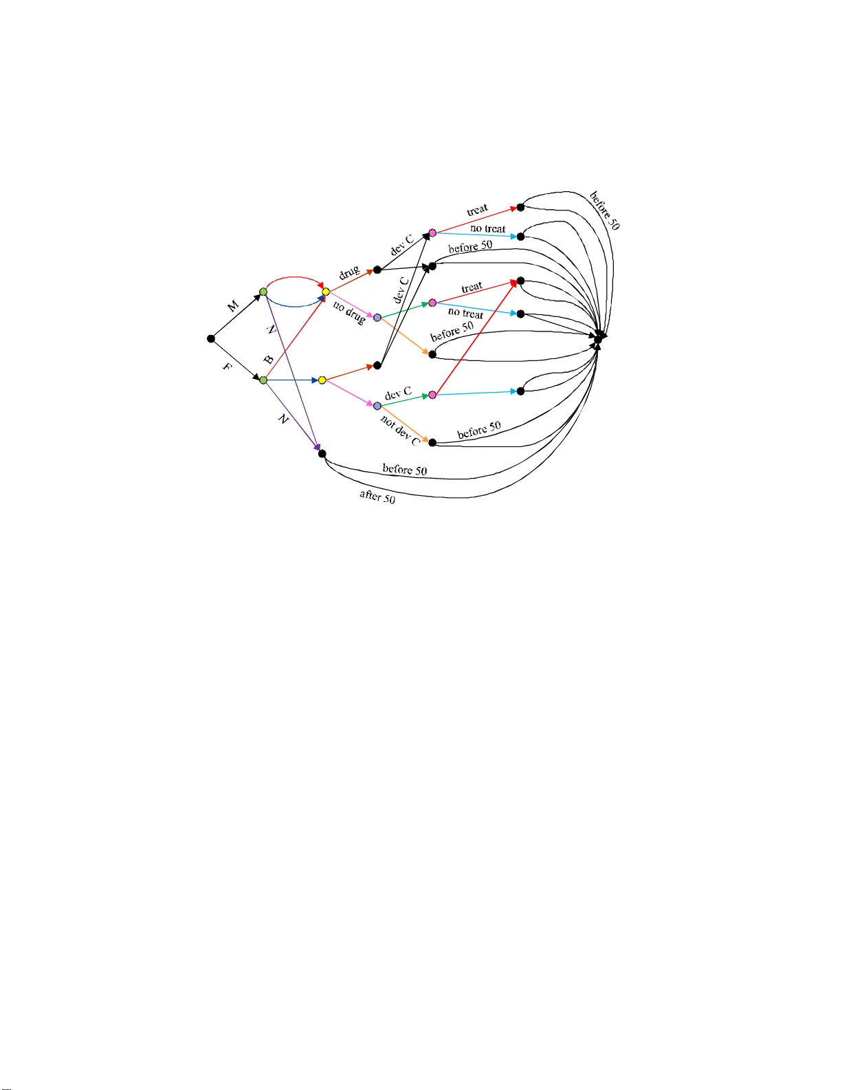
A Separation theorem for Chain Ev en t Graphs P eter Th w aites 1 and Jim Q. Smith 2 1 Univ ersit y of Leeds 2 Univ ersit y of W arwic k Abstract: Ba yesian Net works (BNs) are p opular graphical models for the representation of statistical problems em b ody ing dep endence relationships betw een a num ber of v ariables. Much of this p opularity is due to the d-se pa ration theorem of Pearl and Lauritzen, which al- lows an analys t to iden tify the conditional indep endence statements that a mo del of the pro blem embo dies using only the top ology of the graph. How ev er for man y problems the complete mo del de- pendenc e structure cannot be depicted b y a BN. The Chain Even t Graph (CEG) was in tro duced for these t yp es of problem. In this pa- per we int ro duce a s eparation theor em for CE Gs, analo gous to the d-separa tio n theorem for BNs, which lik ewise allows an analyst to ident ify the conditio nal indep endence str ucture of their mo del from the to polog y of the gr aph. Keyw ords: Bay esian N etw ork, Chain Even t Graph, conditiona l independenc e , directed acyclic gr aph, gra phica l mo del, separation theorem 1 In tro duction If the DA G (directed acyclic gr aph) of a Bay esian Netw ork (BN) has a vertex set { X 1 , X 2 , . . . , X n } , then there are n conditiona l indep endence assertio ns which can simply b e read oﬀ the g raph. These are the proper ties that state that a vertex-v ar iable is independent of its no n-descendants giv en its pa r en ts (the directed lo cal Marko v prop erty [20]). Answering most conditional indep endence queries ho wev er, is not so straight forward. The d-separ ation theorem for BNs was ﬁrst prov ed by V er ma and Pearl [43], and an alternative version co nsidered in [22, 20, 9]. The theor em addresses whether t he conditional indep endence query A ∐ B | C ? can b e answered from the top ology of the DA G of a BN, where A, B , C are disjoint s ubsets of the set o f vertex-v ariables of the DA G. Separation theorems ha ve b e en prov ed for more general classes of g raphical mo del including chain graphs [6], alterna tiv e chain gr aphs [2], and ances tral graphs [3 0]. How ev er, for many problems the a v ailable quantitativ e dep endence infor - mation cannot all b e embo died in the DA G of a BN. The Chain Ev ent Gr a ph 1 (CEG) w as in tro duced in 2006 [39, 38] for the representation & analysis of precisely these so rts of problems. There hav e b een a do z en pap ers on CE Gs published since then, principally conce r ned with their use for problem rep- resentation (eg. [34]), pr obabilit y propaga tion [41], learning and mo del selec- tion [1 4, 15, 3, 3 3, 4, 10], and causal analysis [4 2, 37]. The mo tiv ation for the developmen t of this class is that CE Gs are probably the most natur a l gr aphical mo dels for discre te pro cesses when elicitation inv olves questions ab out how s itu- ations migh t unfold. Although the topo logy o f these gr aphs is more complicated than that of the BN, they a re more expres s iv e, as they allow us to r epresent all str uctural quantitativ e information within the gra ph itself. Context-speciﬁc symmetries which are not intrinsic to the structure of the BN [7, 23, 29, 31] are fully express ed in the top ology of the CEG, which also recog nises logical or structural zero s in pr o babilit y ta bles, and the num be r s of lev els taken by problem-v ariables. This la st has bee n found to b e essential to under standing the geo metry o f B N mo dels with hidden v ariables [1, 26]. In this paper w e re- turn to the mathematics underpinning CEG mo dels, a nd provide a separation theorem for these gr aphs. The CEG is a tree-based graphical structure with a passing resemblance to graphs s uc h as Bozga & Male rs’ proba bilistic decision gr aph [8] (made popula r by Ja eger et al in [1 7]). It diﬀers from these in that edges in a CEG label even ts that might happ en to an individual in a po pulation given a particula r partial history , and the coalescing of vertices & colo uring of edges together en- co de conditiona l independence/Mar k ov structur e. The colouring o f CEGs and their a cyclicit y a lso distinguish them fr o m Mar k ov s ta te space diagrams. Finite CEGs as discussed in this pap er also hav e ﬁnite event s paces whose atoms cor- resp ond to the distinct p ossible histories o r developmen ts that individuals in a po pulation migh t ha ve. The tree-structur e imparts to these atoms an additional longitudinal elemen t consisting of the stages of a n individua l’s developmen t. W e note in pas sing that colour has recen tly been found to pro vide a v aluable em- bellis hmen t to other graphica l models (see for example [16]). Even more so tha n is the case with BNs, ther e ar e a num b e r o f conditional independenc e proper ties which ca n simply b e r e ad oﬀ the CEG [34], a nd g iv en the tree - based nature of the CEG these prop erties a re naturally context-speciﬁc. That is to say they ar e prop erties of the for m A ∐ B | Λ for some even t Λ. An example w ould be that a particular lifest yle-rela ted medical condition is inde- pendent of gender given that the s ub ject is a s mok er. An ana lo gous statement for a discrete BN would be of the form p ( A | B , C = c ) = p ( A | C = c ) for some subsets of v ariables A, B , C , some sp eciﬁc vector v alue c of C and all vector v a lues of A a nd B . The clas s of co nditioning even ts we can tackle with a CEG is how ever muc h richer tha n that genera lly considered when using BN-based analysis. In Section 2 we use a toy example to introduce CEGs. A naive criticism of tree-bas ed gr aphical s tructures is tha t they will b e to o co mplex for la r ger 2 problems. W e note that the pictur e is simply for the inv estigator ’s (or a client ’s) bene ﬁt: as with any large system, analy sts need to consider b oth lo cal and glo bal asp ects – the full CE G for a large pro blem may ex ist only as a set of computer constraints; local asp ects of the problem can b e drawn out as a simple graph. Our example her e is small so that we can use it e ﬀectiv ely to illustr a te key ideas. W e then for mally deﬁne a CEG, and expla in how coalescence & colouring enco de co nditional independence structure. E v ents & rando m v ariables deﬁned on CEGs a re introduced through our example, as are s ub- CEGs conditioned on an event of interest. In Section 3 w e introduce e le mentary v ariables asso ciated with the v ertices of the CEG, and use these to co nstruct a sepa ration theorem. Co mparison with the d-separa tion theorem for BNs is made through cor ollaries and our running example. Section 4 develops s ome of the idea s from earlier s ections. 2 Chain Ev en t Graphs Deﬁnitions of Chain Even t Gra phs (of v arying degrees of complexity) hav e ap- pea red in many of the previo us pa pers on these gr aphs. W e oﬀer a detaile d formal deﬁnition her e so that the theor ems in later sections have a ﬁrm ma the- matical fo unda tion. 2.1 Ev en t T rees W e introduce CE Gs in this sectio n throug h the use o f a toy example, simple enough to illustrate the key ideas. The CEG is a function of an event tr e e [32], and was created to o vercome some of the shortco ming s of these gr a phs. So we s tart by considering an even t tree elic ited fro m some exp e rt. Example 1. A re se ar che r is investigating a p opulation of p e ople whose p ar ents suﬀer er e d fr om an inherite d me dic al c ondition C . S he has information on the gender of e ach individual; if and when they displaye d a symptom S (never, b efor e pub erty, after pub erty); and whether or not they develop e d the c ondition C . Her cu r re nt r ese ar ch is r etr osp e ctive so she also has these individual’s ages at de ath. S he susp e cts that the c onditio n c an le ad to e arly de ath, so she pr o duc es an indic ator that for e ach individual r e c or ds whether or n ot they die d b efo r e the age of 50. She knows that an individual who do es n ot display symptom S wil l not develop the c onditio n. An event tr e e fo r this information i s giv en in Figur e 1. The tr e e is a natur al description o f the problem. The lab els on the edges of each ro ot-to- leaf pa th (eg. male, displa y S b efor e pub erty, develop C , die b efo r e 50 ) in Figure 1 follow a temp oral order, and the absence of c ondition edges in the 9th, 10th, 1 9 th & 20th s uch paths r e ﬂe c ts the exp ert’s knowledge that individuals who do not dis pla y S do not develop C. 3 v 0 v 1 v 2 v 3 v 7 v 5 v 9 S a fter v 10 v 18 v 17 v 4 v 6 v 8 v 36 Figure 1: Event tree for Example 1 An ev ent tree T is a connected directed graph with no cycles. It has one r o ot vertex ( v 0 ) with no pa ren ts, whils t all o ther vertices hav e exactly one par en t. A leaf-vertex is a v ertex with no c hildren. W e denote the vertex set of T b y V ( T ) and the edge set by E ( T ). A directed ro ot-to- leaf path in T is ca lled a r oute . Although an event tre e could be used to re pr esen t an observer’s b eliefs a bout the p ossible dev elopments of some individual, w e ma k e the assumption that the tree relates to a p opulation. Hence the r outes o f the t ree des cribe pr ecisely the p ossible de velopments or histor ies that a n individual in the p opulation ca n exp erience. This descriptio n takes the for m of a sequence of edge-lab e ls, eac h describing what can happen ne x t at a vertex. So in Figure 1 for example, an individual who is male reaches vertex v 1 where the p ossible immediate dev elop- men ts are tha t he displays S befor e pube rt y , after pub erty or not at all. W e sp ecify that the edges leaving a n y vertex in the tree must have distinct lab els; that each individual can only pass along one edge leaving any vertex, and the choice of whic h edge is determined o nly by the v a riable co ntrolling the next stag e of dev elopment (eg. symptom ) and not b y any possible further developmen ts downstream of these edges (ie. towards the leaves). W e also requir e that eac h route corres p onds to a real p ossible developmen t or histor y o f an individual in the p opulation. So each such pa th has a non- zero probability that some individual might take this path. Also, the num ber 4 of ro utes corr e sponds ex actly to the num be r of distinct p ossible his to ries or developmen ts (deﬁned by the e dg e-labe ls) that so me individual could exp erience. Once we ha ve a set of ro utes, and some ordering on these paths, then the edge-lab els deﬁne the tree structure. In our example the ﬁrst v a r iable in our order is gender , so v 0 has tw o emanating edges, la belled male & female . The second v ariable is symptom , so v 1 & v 2 bo th hav e three emana ting edges , labelled displays S b efor e pub erty, di splays S after pub erty & never displays S. W e know that individuals who never display S will not develop condition C, so the edges emanating from v 5 & v 8 lab el the poss ible v alues of the life-exp ectancy indica tor, whereas those emanating from v 3 , v 4 , v 6 & v 7 lab el the pos s ible v alues of c onditio n . In this pap er we use the notation λ to denote a route, and the set of routes of T is lab elled Λ ( T ). When the tree is applied to a population, each route λ corres p onds to a po ssible history or developmen t of an individual in the popu- lation, and hence to an atom in an even t space deﬁned by the tree. The sigma ﬁeld of even ts asso ciated with T is then the set o f a ll p ossible unions o f a toms λ in Λ( T ). No te that the tre e encodes an additional longitudinal dev elopment or history for the individua l, not enc o ded by the sig ma ﬁeld alone [32]. E v ents in the sig ma ﬁeld o f the tree are deno ted Λ. So for instance, in Example 1 the ev ent Λ corresp onding to displaye d S b efo r e pub erty and die d b efor e t he age of 50 is simply the union of the 1st, 3rd, 11th & 1 3th routes in the tre e in Figure 1. Example 1 con tin ued. Ou r r ese ar cher has done suﬃcient analysi s of the data to tel l us that: • life exp e ct ancy of individuals in this p opulation is indep endent of gender given that S is not disp laye d, • males who displa y S at any p oint and females who display S b efor e pub erty have t he same joint pr ob ability distribution over the variabl es condition and life exp ectancy . Mor e over • if and when an indivi dual displays S is indep endent of gende r, and she b elieves tha t • males and females who display S at any p oint have the same pr ob ability of developi ng the c ondition. It is the fact that tra ditional trees cannot rea dily depict this sort o f info r ma- tion which ha s led to tree- based analy sis not receiving the attention it deserves. It is ac tually relatively eas y to po rtray these t yp es of co nditional indep endence or Mar k ov pr operties on a tree – all we need to do is a dd colour to the edges, as in Figure 2 (where edges with the same colouring carry the sa me probability). Despite the c olouring this is s till a rather cumber s ome representation. T o make it mo re compact we use the idea o f c o alesced trees, used in decision anal- ysis since [27]. In a coalesced even t tree v ertices from which the sets of p ossible complete future developments hav e the same pro babilit y distribution a r e c o a- lesced. 5 v 0 v 1 v 2 v 3 v 7 v 5 v 9 after v 10 v 18 v 17 v 4 v 6 v 8 v 36 Figure 2: Coloured e vent tree for Example 1 So in the tree in Figure 2 we can coalesce the vertices v 3 , v 4 & v 6 and a lso the vertices v 5 & v 8 (the vertices v 9 , v 11 & v 13 and v 10 , v 12 & v 14 are also c o alesced, but this coa lescence is in a sense absorb ed into that of v 3 , v 4 & v 6 ). The co m bination of colo uring a nd co alescence g iv es us a more compact g raph that allows us to p ortray a ll co nditional indep endence pro perties of the type describ ed in Example 1 a bov e. So in Figure 3 , the ﬁrst tw o of the four statemen ts provided by our r esearcher are depicted by the coalescence , but the latter tw o req uire the colo uring of the edges leaving v 1 & v 2 and v 3+4+6 & v 7 . The co louring of the edges emanating from v 9+11+13 & fr om v 10+12+14 is suppressed a s it no long er yields an y extra information. 2.2 Probabilities on T rees In section 2.1 w e talked in gener al terms ab out probabilities on trees. In this section we for ma lise these ideas. In Figure 1 the proba bility of the atom { male, displaye d S b efor e pub erty, de- 6 v 0 v 1 v 2 v 3+4+6 v 7 v 5+8 v 9+1 1+13 before after after v 10+12+14 v 15 v 16 Figure 3: Coalesced ev ent tree for Exa mple 1 velop e d C, die d b efor e 50 } is clear ly: p (male) × p (displayed S b efore pub erty | male) × p (develop ed C | male, displayed S b efore pub erty) × p (died b efore 5 0 | ma le, displayed S b efore pub erty , developed C) which can b e wr itten as π e ( v 1 | v 0 ) π e ( v 3 | v 1 ) π e ( v 9 | v 3 ) π e ( v 17 | v 9 ) where π e ( v 17 | v 9 ) is the pr obabilit y of an individua l having r eac hed the vertex v 9 in Figure 1 (ie. they are male, display ed S b efore puber t y & develop ed C) then taking the edg e e ( v 9 , v 17 ) to reach the vertex v 17 (ie. they die befor e 50) etc. W e ca n assign a probability to ea ch ato m of the even t space as: p ( λ ) = Y e ( v,v ′ ) ∈ λ π e ( v ′ | v ) where e ( v , v ′ ) means the edge from vertex v to vertex v ′ , e ( v , v ′ ) ∈ λ means that e ( v , v ′ ) lies on the route λ , and π e ( v ′ | v ) is the co nditional pr obabilit y of trav ersing the edge e ( v , v ′ ) g iv en that have re a c hed the vertex v . W e call the probabilities { π e ( v ′ | v ) } the primitiv e probabilities of the tree T . 7 The se t { p ( λ ) } deﬁnes a pro babilit y measur e ov er the sigma ﬁeld o f ev ents formed b y the atoms λ ∈ Λ( T ). Strictly sp eaking these probabilities are the fundamen tal probabilities of the system as they are the probabilities of the atoms. Ea c h primitive probability has then a unique v alue determined by these { p ( λ ) } . The conditio nal probability of an edge e ( v, v ′ ) is g iv en by: π e ( v ′ | v ) = P λ : e ( v,v ′ ) ∈ λ p ( λ ) P λ : v ∈ λ p ( λ ) where the numerator is the sum of the probabilities of all routes utilising the edge e ( v , v ′ ), and the deno minator is the sum of the probabilities of all routes passing through the start-vertex v of the edge e ( v, v ′ ). So for example in Figure 1 we hav e: π e ( v 17 | v 9 ) = p ( λ 1 ) p ( λ 1 ) + p ( λ 2 ) where λ 1 is the a tom corr e sponding to the ro ute v 0 − → v 17 ( λ ( v 0 , v 17 )) and λ 2 is the atom corres ponding to the route v 0 − → v 18 ( λ ( v 0 , v 18 )). In practice how ever, our elicitation of the tree is likely to yield primitive probabilities o f the sort describ ed ab ov e, rather than probabilities of atoms . 2.3 P ositions and Stages T o a llow our even t tree to encode the full c o nditional indep endence structure of the mo del w e introduce t wo partitions of the tree’s vertices. Let V 0 ( T ) ( ⊂ V ( T )) b e the set of no n-leaf vertices o f T (called sit u ations in [42]). Also let v ≺ v ′ denote that the vertex v pr ecedes the vertex v ′ on some route. Then for an y non-leaf v ertex v a ∈ V 0 ( T ) and leaf-vertex v ′′ a ∈ V ( T ) \ V 0 ( T ) such that v a ≺ v ′′ a , there is a unique s ubpath µ ( v a , v ′′ a ) comprising of the edge s of the route λ ( v 0 , v ′′ a ) which lie b et ween the vertices v a and v ′′ a . Let: π µ ( v ′′ a | v a ) = Y e ( v,v ′ ) ∈ µ ( v a ,v ′′ a ) π e ( v ′ | v ) Now e a c h vertex v ∈ V 0 ( T ) labels a rando m v ariable J ( v ) whose sta te space J ( v ) ca n b e identiﬁed with the set of v − → le af subpaths { µ ( v , v ′′ ) } . Deﬁnition 1. Positions. F or an Event T r e e T ( V ( T ) , E ( T )) , t he set V 0 ( T ) is p artitione d into e quivalenc e classes, c al le d p ositions as fol lows: V ertic es v a , v b ∈ V 0 ( T ) ar e memb ers of t he same e quivalenc e class (p osition) if ther e is a bije ction φ b etwe en J ( v a ) and J ( v b ) such that if φ : µ ( v a , v ′′ a ) 7→ µ ( v b , v ′′ b ) , then (a) the or der e d se quenc e of e dg e-lab els is identic al for µ ( v a , v ′′ a ) and for µ ( v b , v ′′ b ) , (b) π µ ( v ′′ a | v a ) = π µ ( v ′′ b | v b ) . Now, from section 2 .1, tree structure is deﬁned by the e dg e-labe ls, so (a) ab o ve means that the subtrees ro oted in v a and v b hav e identical top ological structure. 8 Similarly , from section 2.2, our e dg e proba bilities a re uniquely deﬁned b y the route pro babilities. W e can se e that the edge probabilities in the subtrees ro oted in v a and v b m ust be uniquely deﬁned by the sets of pro babilities { π µ ( v ′′ a | v a ) } and { π µ ( v ′′ b | v b ) } . So (b) above means that the corresp onding edge probabilities in these tw o subtr e es are equal. So t w o v ertices in a tree are in the same p osition if the sets of poss ible complete future developmen ts fr o m these vertices hav e the same probabilit y distribution. W e denote the set of pos itions o f T by P ( T ) W e no ted ear lier that knowing this par tition of vertices is insuﬃcient for us to fully desc ribe the conditional indep endence structure of the tree, so we int ro duce a second partition. Each vertex v ∈ V 0 ( T ) als o lab els a ra ndo m v ariable K ( v ) whose s tate spa ce K ( v ) can be identiﬁed with the s et of dire c ted edges e ( v, v ′ ) emanating from v . Deﬁnition 2. Stages. F or an Event T r e e T ( V ( T ) , E ( T )) , the set V 0 ( T ) is p artitione d into e quiva lenc e cl asses, c al le d stages as fol lows: V ertic es v a , v b ∈ V 0 ( T ) ar e m emb ers of the same e quivalenc e class (stag e) if ther e is a bije ction ψ b etwe en K ( v a ) and K ( v b ) s u ch that if ψ : e ( v a , v ′ a ) 7→ e ( v b , v ′ b ) , t hen π e ( v ′ a | v a ) = π e ( v ′ b | v b ) . So t wo vertices in a tree are in the same stage if their sets o f emana ting edges hav e the same pro babilit y distr ibution. Note that the set o f stag es is coa rser than the set o f p ositions, and that vertices in the same p osition ar e necessar ily in the same stage. W e also add co louring to trees to illus tr ate the stage structure. So vertices in the same stag e are given the s ame co lour, and edges emanating from v ertices in the same stage a re coloured ac cording to their pr o babilities / lab els. This induces a par tition on E ( T ). 2.4 Chain Ev en t Graphs The Chain Event Gr aph C is a direc ted ac y clic gr a ph (DA G), which is connected, having a unique r o ot vertex (with no incoming edges) and a unique si nk vertex (with no outgo ing edges). Unlik e the BN mor e than o ne edge can e x ist b e- t ween tw o vertices of a CEG. The C E G also generally has its v ertices and edg es coloured, a lthough most of this pap er will deal with uncoloured versions c a lled Simple CE Gs . The ro ot and sink vertices of a CEG are lab elled w 0 and w ∞ . Deﬁnition 3 . Chain Even t Graph. The CEG C ( T ) (a fun ct ion of the tr e e T ( V ( T ) , E ( T )) ) is the gr aph with vertex set V ( C ) and e dge set E ( C ) deﬁne d by: 1. V ( C ) ≡ P ( T ) ∪ { w ∞ } ; 2. (a) F or w, w ′ ∈ V ( C ) \ { w ∞ } ther e is a dir e cte d e dge e ( w , w ′ ) ∈ E ( C ) iﬀ ther e ar e vertic es v , v ′ ∈ V 0 ( T ) such t hat the vert ex v is in the p ositio n w ( ∈ P ( T ) ), v ′ is in t he p osi tion w ′ ( ∈ P ( T ) ), and ther e is an e dge e ( v , v ′ ) ∈ E ( T ) ; 9 w 0 w 1 w 2 w 3 w 4 w 5 w inf w 6 m a l e f e m a l e before after n e v e r b e f o r e after n e v e r d e v e l o p C n o t d e v e l o p C d e v e l o p C n o t d e v e l o p C b e f o r e 5 0 after 50 b e f o r e 5 0 a f t e r 5 0 w 7 w 8 w 9 Figure 4: CEG for Example 1 (b) F or w ∈ V ( C ) \{ w ∞ } t her e is a dir e cte d e dge e ( w , w ∞ ) ∈ E ( C ) iﬀ t her e is a vertex v ∈ V 0 ( T ) such that v is in the p osition w ( ∈ P ( T ) ), and t her e is an e dge e ( v , v ′ ) ∈ E ( T ) for some le af -vertex v ′ ∈ V ( T ) \ V 0 ( T ) . Note that the vertex set o f C ( T ) consists of the p ositions of T and the sink- vertex w ∞ . Positions in C ( T ) ar e sa id to b e in the s a me stage if the comp onent vertices (in T ) o f these positio ns are in the same stage. Colour ing in C ( T ) is inherited from T . The constraints a sso ciated with the positions & stages o f a CEG ho ld for the entire po pulation to which the CEG has b een applied, Example 1 con ti n ued. T o c onvert the c o alesc e d tr e e fr om Fi gur e 3 to a CEG is stra ightforwar d. We simply c ombine the le af-vertic es into a sink-vertex w ∞ as in Figur e 4. The p ositio ns he r e ar e w 0 thr ough w 9 . We note that w 1 & w 2 ar e in the same st age (as c an b e se en fr om the c olouring), w 3 & w 4 ar e in t he same stage, and e ach of w 5 thr ough w 9 is in a stage by itself. The p osition w 3 enc o des the c onditio nal indep endenc e / M arkov pr op erty that males who display S at any p oint and fe males who display S b efor e pub erty have t he same joint pr ob ability distribution over the variabl es condition and life exp ectancy . The p ositio n w 5 enc o des the pr op erty that life exp e ctancy of indi- viduals in this p op ulation is indep endent of gender given that S is not displaye d. The stage { w 1 , w 2 } enc o des the pr op erty that i f and when an individual dis- 10 plays S is indep en dent of gender. The stage { w 3 , w 4 } en c o des the pr op erty t hat condition is indep endent of gender given S displaye d. Without ambiguit y we simplify our notation C ( T ) to C . Analogously with the tree, a directed w 0 → w ∞ path λ in C is c a lled a r oute . The se t of ro utes of C is la belled Λ( C ). W e write w ≺ w ′ when the positio n w precedes the p osition w ′ on a route. When the CE G is applied to a p opulation, ea c h route λ co r resp onds to a po ssible history or developmen t of an indiv idua l in the p opulation, and hence to an atom in the even t space deﬁned by the CEG. The sigma ﬁeld of even ts asso ciated with C is then the set of a ll poss ible unions of atoms λ in Λ( C ). Like the tree , the CEG enco des a n additional longitudinal developmen t or histo ry for the individual, no t encoded by the sigma ﬁeld alone. Event s in the sigma ﬁeld of the CEG are deno ted Λ. Note that the n um b er of ro utes in the CEG equals the num b er in the tree and corres p onds exactly to the n umber of p ossible distinct historie s o r developments that some individua l in the population could exp erience. And since no route has a zero pro babilit y , all edges in the CEG have non-zer o co nditional probabilities asso ciated with them. Because the CEG’s atoms ha ve this implicit lo ngitudinal developmen t asso- ciated w ith them, certain ev ents in the sig ma ﬁeld are par ticularly imp ortant. Let Λ( w ) de no te the even t that an individual unit takes a r oute that pa sses through the p osition w ∈ V ( C ). Λ( w , w ′ ) is then the union of a ll routes passing through the positio ns w a nd w ′ , Λ( e ( w , w ′ )) is the union of all ro utes pa ssing through the edge e ( w , w ′ ), and Λ( µ ( w, w ′ )) is the union of all ro utes utilising the s ubpath µ ( w, w ′ ). 2.5 Probabilities on CE Gs As with tr e es, under lying the CE G there is a probabilit y s pace which is sp eciﬁed by assig ning pro babilities to the atoms. F or each p osition w ∈ V ( C ) \ { w ∞ } and edg e e ( w , w ′ ) emanating from w , we denote b y π e ( w ′ | w ) the pro ba bilit y of tr aversing the edge e ( w , w ′ ) conditional on having rea c hed the po sition w . W e call the probabilities { π e ( w ′ | w ) : e ( w, w ′ ) ∈ E ( C ) , w ∈ V ( C ) \{ w ∞ }} the primitive pr ob ab ilities of C . Then, analogous ly with trees, for each atom λ : p ( λ ) = Y e ( w,w ′ ) ∈ λ π e ( w ′ | w ) as bo th the atoms and the pr imitiv e probabilities are iden tical to the co rre- sp onding atoms and pr imitiv e probabilities in the tree. The se t { p ( λ ) } deﬁnes a pro babilit y measur e ov er the sigma ﬁeld o f ev ents formed by the atoms λ ∈ Λ( C ). This assignment of pro babilities implicitly demands a Mar k ov pr oper t y over the ﬂow o f the units t hroug h the graph. Th us, in the context of our medi- cal example, the probablility of an individual with attributes ( male, displaye d 11 symptom S b efor e pub erty ), ( male, displaye d symptom S after pub erty ) or ( f e- male, d isplaye d symptom S b efo r e pub erty ) de veloping the co ndition dep ends only on the fact that the subpaths cor r espo nding to these pairs of attributes terminate a t the p osition w 3 , and not on the particular subpath leading to w 3 . The probability this individual develops the condition is then π e ( w 6 | w 3 ) ≡ p (Λ( e ( w 3 , w 6 )) | Λ( w 3 )). So we only need to know the position a unit has reached in order to predict as well as is p ossible what the next unfolding of its developmen t will b e. This Markov hypothesis lo oks stro ng but in fact holds for many families o f statistical mode l. F or example all ev ent tree descr iptions of a pro ble m satisfy this prop erty , all ﬁnite state space context speciﬁc Bayesian Netw orks as well as ma n y other structures [34]. W e can go further and s tate that the sets of p ossible future developmen ts (whether o r not they developed the c o ndition and whether or no t they died befo re the a ge of 50) for individuals ta k ing any of these three subpaths m ust be the same. Moreover the conditional probability of any particular subsequen t developmen t must be the sa me for indiv idua ls taking any of these thr ee sub- paths. Note also that if po s itions w a and w b are suc h that the sets of p ossible future developmen ts fro m w a and w b are identical, and the conditional joint probability dis tr ibutions over these s e ts ar e identical, then w a and w b are the same p osition, and m ust be coa lesced for our graph to be a CE G. The probability of a ny even t Λ in the sigma ﬁeld is hence of the form p (Λ) = X λ ∈ Λ p ( λ ) = X λ ∈ Λ Y e ( w,w ′ ) ∈ λ π e ( w ′ | w ) where λ ∈ Λ means that λ is one of the co mponent atoms of the even t Λ. In this pap er we will a lso use the fo llowing further notatio n: π µ ( w ′ | w ) ≡ p (Λ( µ ( w , w ′ )) | Λ ( w )) denotes the pr obabilit y of utilising the subpath µ ( w , w ′ ) (co nditional on passing through w ), π ( w ′ | w ) ≡ p (Λ( w , w ′ ) | Λ( w )) = P µ π µ ( w ′ | w ) deno tes the pr obabilit y of arriving at w ′ conditional on pass ing through w . Expressing a pro blem as a CEG allows domain exper ts to check their beliefs in a very straig h tforward manner : W e stated in Section 2.1 that the ex pert in our example b elieved that males & females w ho display S at an y point have the same probabilit y of developing C. This is depicted in the colo uring of the edges ema nating fro m w 3 & w 4 in Fig- ure 4. O ur expe r t can now use the techniques developed in [14, 15, 3, 33] to tes t the model repre s en ted by Figur e 4 aga inst a lternativ e models with diﬀerent con- ditional indep endence / Markov structure. Such a test might yield information that groupe d the v ertices v 3 , v 4 , v 6 & v 7 from Figure 1 into diﬀerent positio ns than thos e in Figure 4; or that the v ertices v 3 , v 4 & v 6 are indeed in the same stage and positio n, but that the vertex v 7 is not in this stage (ie. the pr obabilit y of dev eloping C is diﬀere n t for female s who display S after pub erty), a nd so the edges leaving w 3 & w 4 in Figure 4 would no lo nger have the same colouring . 12 2.6 Conditioning on even t s Most conditional indep endence queries that could r ealistically b e of interest to an a nalyst can be answered purely by insp ecting the top ology of a CE G. And most of these queries in volv e conditioning on w ha t is known as an intrinsic even t. Deﬁnition 4. Intrinsic ev en ts. L et C Λ b e t he sub gr aph of C c onsisting of only those p ositions and e dges that lie on a r oute λ ∈ Λ , and the sink-vertex w ∞ . Λ is in trinsic to C if the numb er of w 0 − → w ∞ p aths in C Λ e quals the numb er of atoms i n the set { λ } λ ∈ Λ . The idea of intrinsic even ts is closely related to that of fa ithfulness in BNs [24, 36]. Note that each atom (& therefore edge) in C Λ m ust b y construction have a non-zer o probability , but edge-probabilities in C Λ may diﬀer from thos e in C since so me vertices in C Λ will hav e few er emanating edges than they hav e in C , and the proba bilities on the emana ting edges of any vertex must sum to one. All ato ms of the sigma ﬁeld of C are intrinsic, a s are Λ( w ), Λ( w , w ′ ), Λ( e ( w , w ′ )), Λ( µ ( w, w ′ )) (provided these are non-empty), and as is the exha ustiv e set Λ( w 0 ). If we include the empt y set in the set of intrinsic e v ents then we note that in- trinsic sets a re closed under in tersectio n and so tech nically fo rm a π - system (see for ex ample [18]) we can asso ciate with the CE G C . Not all ev ents in the sigma ﬁeld ar e necessarily in trinsic, beca use the class of int rinsic even ts is not clo sed under union. F or example, for the CEG in Figure 4, the even t Λ co ns isting of the union of the t wo atoms describ ed by the routes male, displ ay S b efo r e pub erty, develop C , die b efor e 50 a nd male, display S after pub erty, develop C , die after 50 pr oduces a s ubgraph C Λ which has four distinct routes, so Λ is no t intrinsic. How ever, our int erest in intrinsic ev ents is that we can condition on them, and we show below that conditioning o n in trinsic ev ents often destroys the stag e-structure of C . Conditioning on non- intrinsic e vents usually destroys p o sition-structure. F rom this w e ar g ue tha t if we know that w e wish to condition on a n ev ent such a s the one describ ed above, w e would simply sacriﬁce the p osition-structure of our CEG (knowing tha t it would pr obably be lost in the conditio ning anyw ay) and split (uncoalesce ) the p osition w 3 to form a g raph for which this event is intrinsic. Even without s uch sleight o f hand, the class of intrinsic e vents is r ic h enough to encompass vir tually all of the conditioning even ts in the conditional indep en- dence statements we would like to query . In particula r , if our mo del can b e expressed as a BN (with vertex-v ariables { X j } ) then any set of obs erv a tio ns ex- pressible in the form { X j ∈ A j } ( { A j } subsets of the sample spaces of { X j } ) is a prop er s ubset o f the set of intrinsic even ts deﬁned on the CEG of o ur mo del [41]. Example 1 con tin ued. Supp ose for il lustr ative c onvenienc e that t he e dges la- b el le d male, female, display ed S b efore pube r t y , displayed S after pub ert y , nev er display ed S, develop ed C, did not develop C in our CEG have t he pr ob abilities 1 2 , 1 2 , 1 4 , 1 4 , 1 2 , 1 2 , 1 2 . Now le t u s c ondi tion on the event Λ which is the u nion of al l r outes except { female, display ed S after pube r t y , did not develop C, die d 13 befo re 50 } and { female, display ed S after puber t y , did not develop C, died after 50 } . This event Λ is cle arly i ntrinsic to C , and has the p r ob ab ility p (Λ) = 15 16 . When we c ondition on Λ , the r outes λ which ar e c omp onents of Λ get new pr ob abilities p ( λ | Λ) = p ( λ, Λ) /p (Λ) = p ( λ ) /p (Λ) . In this c ase e ach r oute has its pr ob abi lity mult ipl ie d by 16 15 . We le ave it as a (simple) exer cise to sho w that al l e dge-pr ob abilities r emain unchange d exc ept: π e ( w 1 | w 0 ) b ecomes 8 / 15 π e ( w 2 | w 0 ) b ecomes 7 / 15 π e ( w 3 | w 2 ) b ecomes 2 / 7 π e ( w 4 | w 2 ) b ecomes 1 / 7 π e ( w 5 | w 2 ) b ecomes 4 / 7 π e ( w 8 | w 4 ) b ecomes 1 the e dge π e ( w 9 | w 4 ) do es not exist in C Λ So the p ositions w 1 and w 2 ar e no longer in the same stage. So, as alrea dy noted, co nditioning on an in trinsic even t ca n destro y stage- structure. This leads us to deﬁne an uncoloured version of the CEG. Deﬁnition 5. Simpl e CEG A simple CEG (sCEG) is a CEG wher e ther e ar e no c onstr ai nts on e dge-pr ob abilities, exc ept that (i) al l e dge-pr ob abilities must b e gr e ater than zer o (a c onse qu enc e of the r e quir ement we made for tr e es), and (ii) the sum of emanating-e dge-pr ob abilities for any p osition must e qual one. What this means in practice is that sta ge-structure is suppr essed: there a re no stages whic h a re not p ositions, and so colouring is r e dundan t. There is an analogy here with BNs to which one can always add edges, and sacriﬁce a little conditional independence str uc tur e. W e s ho w now that the cla ss of sCE G mo dels is closed under co nditio ning on an intrinsic even t: Theorem 1. F or an event Λ , intrinsic to C , the sub gr aph C Λ is an sCEG. If the pr ob ability of any r oute λ in the sigma ﬁ eld of C Λ is given by p Λ ( λ ) = p ( λ | Λ) , then the e dge-pr ob abilities in C Λ ar e given by: ˆ π e ( w ′ | w ) = p (Λ | Λ( e ( w, w ′ ))) p (Λ | Λ( w )) π e ( w ′ | w ) The pr o of o f this theo rem is in the a ppendix. W e note that this result has bee n success fully used to develop fast propag a tion algorithms for CEGs [41]. Note that the pro babilit y o f an atom λ in C conditioned on the intrinsic even t Λ is the probability of that a tom in the sCEG C Λ (denoted p Λ ( λ )). It is then trivially the case that the probability of an ev en t in C conditioned on the even t Λ is the pro babilit y of that even t in the sCEG C Λ . 14 2.7 Random v ariables o n sCE Gs Random v ariables measurable with resp ect to the s igma ﬁeld of C partition the set of atoms into even ts. So consider a random v ariable X with state space X , and let us denote the even t that X takes the v alue x ( ∈ X ) by Λ x . Then the set { Λ x } x ∈ X partitions Λ( C ). F or any CEG there is a set of fair ly tra nsparent random v ariables which includes as a subset the set of measurement v a riables of any B N- r epresentation of the mo del, if such a representation exists. Thes e are called cu t-variable s and are dis c us sed in detail in Section 3 .2 . In Figure 4 for example, we hav e a v ar iable which could be called symptom , whic h co uld tak e the v alues 1, 2 & 3 (in some order) for routes tra versing edges labe lle d b efor e , after and never . These are not how ever the only v ariables w e can deﬁne on a CEG, and we ﬁrst co nsider some results for ge ner al v a riables. Note that when w e write X ∐ Y we mean that p ( X = x, Y = y ) = p ( X = x ) p ( Y = y ) ∀ x ∈ X , y ∈ Y , and that this is tr ue for all distributions P compatible with C . Now for a n in trinsic event Λ, w e can write X ∐ Y | Λ if and only if p ( X = x, Y = y | Λ ) = p ( X = x | Λ) p ( Y = y | Λ) for all v alues x of X and y of Y (see for ex ample [12]). That is X ∐ Y | Λ ⇔ p (Λ x , Λ y | Λ) = p (Λ x | Λ) p (Λ y | Λ) for all Λ x ∈ { Λ x } x ∈ X , Λ y ∈ { Λ y } y ∈ Y . Lemma 1. F or a CEG C , variables X, Y me asur able with r esp e ct to the sigma ﬁeld o f C , and intrinsic c onditioning event Λ , the statement X ∐ Y | Λ i s true if and only if X ∐ Y is tru e in the sCEG C Λ . The pro of of this lemma is in the app endix. This is a particula rly useful prop erty b ecause it allo ws us to chec k any co n text-sp eciﬁc conditiona l inde- pendenc e prop erty by c hecking a no n-conditional independence pr oper t y on a sub-sCEG. T o motiv ate the theory in the remainder o f section 2 and in sectio n 3, we need a bigg er example. Example 2 . O ur r ese ar cher fr om Example 1 now turns her attention to a n ongoing stu dy. Subje cts who display the symptom S (at any p oint) may b e given a drug, and the pr ob ability of r e c eiving this drug is not dep endent on their gender or when they displa ye d S . Those that develop t he c ondition C may b e given tr e atment, and the pr ob ability of re c eiving t his tre atment is not dep endent on their gender, when they displaye d S , or whe ther or not they r e c eive d the e arlier drug. The CE G for this is given in Fi gur e 5. These two pr op ert ies ar e depicte d in the CEG by the p ositions w 3 & w 4 b eing in the same stage, and by w 10 , w 12 & w 14 also b eing in the same stage. Figur e 5 also tel ls us that tr e atment and life exp e ctancy ar e indep endent of gender and when S display e d, giv en b oth the event drug given & develop C and the event drug given & not develop C (the p osi tions w 10 & w 11 ); and that life exp e ctancy is indep endent of gender and when S displa ye d given the event drug not given, develop C & treatment given (t he p ositio n w 18 ). 15 w 0 w 1 w 2 w 3 w 4 w 5 w i nf w 6 B A A after 50 w 7 w 8 w 9 w 10 a fter 50 af ter 50 after 50 w 11 w 12 w 13 w 14 w 15 w 16 w 17 w 18 w 19 w 20 Figure 5: CEG for Example 2 Our r ese ar cher is int er est e d in the r elationships b etwe en c ondition & gender, and b etwe en c ondition & when S displaye d, for the s u b gr oups (i) who wer e given the drug, and (ii) who di splaye d S but wer e not given the d rug. In BN-theory , if we wish to answer the query X ∐ Y | Z ?, one wa y we might sta rt doing this is b y dr a wing the ancestral gra ph of { X , Y , Z } (see for example [21]). W e do this b ecause v ariables in the BN which are not pa rt of this graph hav e no inﬂuence on the o utcome of our quer y . There is no dir ect a nalogy for this graph in CEG-theory , but we can consider a pseudo-a ncestral gra ph a sso ciated with a set of ev en ts or v ariables. So in Example 2 , a ll edges a ssoc ia ted with trea tmen t or life ex pectancy lie downstream (ie. tow ards the sink-no de) of the edg es asso ciated with gender, symptom, dr ug and c o ndition, so we ca n simply curtail our CEG so that it do es not include these edge s. So in Figure 5 , the p ositions w 5 , w 10 , w 11 , w 12 , w 13 , w 14 & w 15 are coa lesced int o a new sink-node w ∞ as in Figure 6. But w 7 & w 9 in Figure 5 w ere in the same stage. As these no des a re no w only one edge upstream o f w ∞ , they get coalesced in to a single new po sition ( w 7 in Figure 6). Notice how m uch simpler the ps eudo-ancestral gra ph is than the orig inal CEG. W e have noted ab o ve that stage- s tructure is often des tro yed by conditio ning on an in trinsic even t, but that the set of s C E Gs is clos e d under this conditioning. 16 w 0 w 1 w 2 w 3 w 4 w 5 w i nf w 6 B A N A dev C dev C not dev C w 7 Figure 6: Pseudo-a ncestral graph for Example 2 So the remainder of our analysis is conducted on an unco loured CEG. The graph in Figure 7 is the uncolo ured pseudo- ancestral sCE G C asso ciated with the queries that our resear cher is interested in. This gr aph is analo gous to the mo ralised ancestra l graph us ed in BN-based a nalysis. There are tw o na tural v ariables whic h pa r tition Λ( C ) – these are ge nder (whic h pa r titions Λ( C ) in to events whic h we will ca ll M (male ) & F (female)), and symptom (which partitions Λ( C ) into ev ents which w e will call B (S displayed befo re pub ert y), A (S displayed a fter pub erty) & N (S never display ed)). The v ariable as socia ted with giving the drug par titio ns Λ ( C ) into three even ts – drug g iven, S display ed but drug not given, a nd S not dis played and hence drug not giv en. As the third of th ese even ts is exactly the event N ab ov e, w e will for brev it y describ e the second even t (particularly when lab elling edg es) simply as drug not given or no drug . The v ar iable asso ciated with c o ndition C partitions Λ( C ) into three even ts – C developed, S display ed but C no t developed, a nd S no t dis pla yed a nd hence C not developed. Again, as the third of thes e even ts is exactly the even t N, we will for bre v it y descr ibe the se cond even t simply as C no t develop ed. There is no am biguity here as the queries our resea rc her is interested in corres p ond to conditioning on the even ts dr ug given, and S display ed but dr ug not given. Her ﬁrst question co ncerns the rela tio nship b et ween condition and when S display ed for the subgr oup who w ere given the dr ug. This re q uires conditioning on the even t drug g iv en, so we dra w the sub-sCEG C Λ for this even t. This is given in Figure 8. The r elationships she is interested in co ncern the proba bilities p Λ (C de velop ed | B) 17 w 0 w 1 w 2 w 3 w 4 w 5 w i nf w 6 B A N A dev C dev C not dev C w 7 Figure 7: Ps eudo-ancestral sCEG C for Example 2 and p Λ (C developed | A), and these a r e given below: p Λ (C de velop ed | B) = { p Λ (M) p Λ (B | M) × 1 × p Λ (C de velop ed | (M , B) or (M , A) or (F , B)) + p Λ (F) p Λ (B | F) × 1 × p Λ (C de velop ed | (M , B) or (M , A) or (F , B)) } ÷ { p Λ (M) p Λ (B | M) + p Λ (F) p Λ (B | F) } = p Λ (C de velop ed | (M , B) or (M , A) or (F , B)) = p (C develop ed | ((M , B) or (M , A) or (F , B)) , drug g iv en) (2 . 1) Note: 1. W e do no t need fo r our purpos es here to ev aluate the p Λ ( . . . ) proba bilities, but if w e wished to w e c o uld use the expression fro m Theorem 1. 2. The e x pression (2 .1) is s till the simplest expr ession even if we were to reintroduce stage-str ucture and let w 1 & w 2 be in the same stage. p Λ (C de velop ed | A) = { p Λ (M) p Λ (A | M) × 1 × p Λ (C de velop ed | (M , B) or (M , A) or (F , B)) + p Λ (F) p Λ (A | F) × 1 × p Λ (C de velop ed | F , A) } ÷ { p Λ (M) p Λ (A | M) + p Λ (F) p Λ (A | F) } which clearly do es not equal e x pression (2.1). 3. The denominator is of course p Λ (A), but even if we let w 1 & w 2 be in the same s tage, the ab ov e expression o nly simpliﬁes to 18 w 0 w 1 w 2 w 3 w 4 w 5 w i nf w 6 B A A dev C dev C not dev C Figure 8: C Λ for Λ = { drug g iv en } p Λ (M) p Λ (C de velop ed | (M , B) or (M , A) or (F , B))+ p Λ (F) p Λ (C de velop ed | F , A), which still do es not equal expression (2 .1). Suppo se we now consider the subgroup who display ed S but were not given the drug and the s ub-sCEG C Λ for the even t dr ug not given. This CEG is given in Figure 9 . The corresp onding pro babilities are: p Λ (C de velop ed | B) = { p Λ (M) p Λ (B | M) × 1 × p Λ (C de velop ed) + p Λ (F) p Λ (B | F) × 1 × p Λ (C de velop ed) } ÷ { p Λ (M) p Λ (B | M) + p Λ (F) p Λ (B | F) } = p Λ (C de velop ed) = p (C dev elop ed | drug not given) p Λ (C de velop ed | A) = { p Λ (M) p Λ (A | M) × 1 × p Λ (C developed) + p Λ (F) p Λ (A | F) × 1 × p Λ (C de velop ed) } ÷ { p Λ (M) p Λ (A | M) + p Λ (F) p Λ (A | F) } = p Λ (C de velop ed) = p (C dev elop ed | drug not given) So we hav e that whether C develop e d is indep endent of when S d isplaye d, given that S wa s displa ye d but the drug was not given . 4. W e do not need to consider the case where S never display ed, as this has no intersection with Λ: Given that S displaye d but drug not given , I know that S was display ed, but further knowledge o f when it was displa yed is irrelev ant for prediction of whether o r not the sub ject develop ed C, 19 w 0 w 1 w 2 w 3 w 4 w i nf B A A w 7 Figure 9: C Λ for Λ = { drug not given } 5. This cont ext-sp eciﬁc conditional indep endence pro perty ho lds whether or not we reintroduce sta ge-structure and let w 1 & w 2 be in the same stag e. Let us now consider our r esearcher’s other queries to do with the relationship betw een condition and gender for our subg roups. F r o m Fig ur e 8 w e can see that if Λ = { drug g iv en } then: p Λ (C de velop ed | M) = p Λ (A o r B | M) × 1 × p Λ (C de velop ed | (M , B) or (M , A) or (F , B)) (2 . 2) and p Λ (A o r B | M) = 1, since A & B ar e the only e dges leaving w 1 in C Λ . p Λ (C de velop ed | F ) = p Λ (B | F) × 1 × p Λ (C de velop ed | (M , B) or (M , A) or (F , B)) + p Λ (A | F) × 1 × p Λ (C de velop ed | F , A) which clearly do es not equal expression (2.2), and this is true ev en if we r ein- tro duce stage- structure and let w 1 & w 2 be in the same stage. F rom Fig ur e 9 we can s e e that if Λ = { drug not given } then: p Λ (C de velop ed | M) = p Λ (A o r B | M) × 1 × p Λ (C developed) = p Λ (C de velop ed) = p (C dev elop ed | drug not given) p Λ (C de velop ed | F) = p Λ (B | F) × 1 × p Λ (C de velop ed) + p Λ (A | F) × 1 × p Λ (C de velop ed) = p Λ (C de velop ed) = p (C dev elop ed | drug not given) 20 So we hav e that whether C develop e d is indep en dent of gender, given t hat S was displaye d, but the drug was n ot given , and this is true irres pective o f whether we reint ro duce s tage-structure. W e notice that the topolog ical feature whic h distinguishes Figur e 9 from Figure 8 is that in Fig ur e 9 there is a cut-vertex (a sing le v ertex not w 0 or w ∞ , through whic h a ll ro utes in the g raph pass) lying betw een the edg es asso ciated with gender & sy mptom (upstrea m) and those asso ciated with condition (do wn- stream). W e return to cut-vertices a nd to their role in indep endence queries in section 3 . Note also that the example ab ov e g iv es ample justiﬁcation for w orking with sCEGs when considering co nditional indep endence queries , ra ther than their coloured co un terparts. 3 A separation theorem for simple CEGs In section 2.7 we int ro duced r andom v ariables on sCEGs. In section 3.1 we de- velop this idea, before providing a separ a tion theorem for sCEGs in sectio n 3.2 . 3.1 P osition v ariables As noted in Section 1, mo diﬁed BNs o f one type or ano ther are widely used b e- cause r e a l problems tend to contain more sy mmetries than ca n be represented by a standar d BN. What is generally no t addressed in pa pers on these type s of gra phs is the conse quence that this extra s tructure has for the Marko v re- lationships b et ween the pro blem v ariables. With CEGs w e can addr e ss this explicitly & automatically , and the ﬁrst step towards doing this is to consider mo del v a riables which are more fundamental than the measurement v aria bles customarily considered when working with BNs. So in this section we describ e t wo types of elemen tary random v ar iables, mea surable with resp ect to the sigma ﬁeld of C , that can b e iden tiﬁed with each p o sition w ∈ V ( C ) \ { w ∞ } . Thes e are the v ariables { I ( w ) }} and { X ( w ) } deﬁned b elow. Note that when we say that a v a riable X takes the v alue x , this is equiv alent to s aying that an individual from o ur populatio n has a developmen t which we equate with a route λ , and that this r oute λ is an ele ment of Λ x , th e even t corres p onding to X = x . F or a pos ition w , I ( w ) ca n take the v alues 1 or 0 dep ending on whether this individual is on a route λ which do es o r do es not pass through w . So: I ( w ) =  1 if w ∈ λ 0 if w 6∈ λ (where a s ab ov e, w ∈ λ means that the p osition w lies on the route λ ). Up until now we have lab elled e dg es by their start and endp oints (eg. e ( w, w ′ )), but we can also label the edges leaving a position w by a set o f 21 arbitrar y lab els of the for m e x ( w ) ( x = 1 , 2 , . . . ). W e deﬁne X ( w ) by: X ( w ) =  x if e x ( w ) ∈ λ 0 if w 6∈ λ So X ( w ) = x ( 6 = 0) if our individual is o n a route λ which passes throug h w and the edge e x ( w ). Recall that a CE G depicts all p ossible histories o f a unit in a po pulation, and gives a probability distribution ov er these histories. How ever, when a single unit trav erses one o f the routes in the CEG, v a lues are assigned to I ( w ) & X ( w ) for a ll p ositions w ∈ V ( C ). Notice that since I ( w ) is clearly a function of X ( w ), to sp ecify a full joint distribution o ver the p osition v ariables, it is suﬃcien t to s pecify the joint dis- tribution of { X ( w ) : w ∈ V ( C ) \ { w ∞ }} . Note als o that all a toms λ can b e expressed a s an in tersection: λ = \ w ∈ λ { X ( w ) = x λ } , and event s in the sig ma algebr a o f C as the union of these atoms: Λ = [ λ ∈ Λ ( \ w ∈ λ { X ( w ) = x λ } ) , where x λ ( 6 = 0) is the unique v alue of X ( w ) lab elling the edge in the route λ . Up until this po in t we hav e used the words upstr e am and downstr e am rather lo osely – in the context o f sets o f edges w e ha ve simply used these words to mean further tow ards w 0 and further tow ards w ∞ ; but we need to for malise the meanings here in the co n text of p ositions . So when we sa y that w 1 is upstream of w 2 , or w 2 is downstream of w 1 , we mea n that w 1 ≺ w 2 . F or an y set A ⊂ V ( C ), let X A denote the set of random v ariables { X ( w ) : w ∈ A } and I A the set { I ( w ) : w ∈ A } . Also, for any w ∈ V ( C ), let U ( w ) be the set of pos itions in V ( C ) which lie ups tream of the p osition w , D ( w ) the set of p ositions whic h lie do wnstream of w , U c ( w ) the set of p ositions whic h do not lie upstrea m of w , and D c ( w ) the set of p ositions which do no t lie downstream of w . Lemma 2. F or any sCEG C and p osition w ∈ V ( C ) \{ w ∞ } , the variables I ( w ) , X ( w ) ex hibit the p osition indep endence prop erty t hat X ( w ) ∐ X D c ( w ) | I ( w ) This result (an extensio n of the Limited Memor y Lemma o f [37]) is anal- ogous to the Directed Marko v pro perty whic h can be used to deﬁne BNs (see for example [28]), a nd whic h states that a BN vertex-v ar iable is indep endent of its non-descenda n ts given its par en ts. It provides a set of conditional indepen- dence statemen ts that can simply b e read from the gr a ph, one for each po sition in V ( C ). The pro of of the lemma is in the app endix. 22 The statement that X ( w ) ∐ X D c ( w ) | ( I ( w ) = 1) can be rea d as: Give n a unit r e ach es a p osition w ∈ V ( C ) , whatever happ ens imme diately after w is indep endent of not only al l develop ments thr ough whic h t hat p osition was r e ache d, but also of al l p ositions that lo gic al ly have not happ ene d or c ould not now happ en b e c aus e the unit has p asse d thr ough w . 3.2 Theorem and corollaries It is doubtful whether BNs w ould hav e enjoy ed their enormous p opularity if it were not so apparently easy to re a d co nditional indep endence prop erties fro m them. In par ticular, the existence of the d-separation theorem [22, 43] has allow ed all pra ctitioners to make some attempt at mo del interpretation with some deg ree of conﬁdence. The pr esence of any con text-sp eciﬁc conditiona l indep endence struc tur e how- ever severely hamp ers analysts us ing BNs in t heir attempts to get accur ate pictures of the structure of their problems [7, 2 9]. In ear lie r s ections of this pap er (a nd in par ticula r in section 2.7 ) we hav e b een developing the th eor y needed for re a ding and represe n ting (co n text-sp eciﬁc) conditional indep endence structure using CEGs. In pa rticular, Lemma 1 allows us to consider co ntext- sp eciﬁc queries by lo oking at the relev an t sub-CE G; and Example 2 pr o vides the rationale for loo king at sCEGs. W e now pr ovide a separa tion theorem for sCEGs. Using the standar d terminolog y of non-pro ba bilistic graph theory , we call a p osition w ∈ V ( C ) \ { w ∞ } a cut-vertex if the remov al of w and its asso ciated edges from C would result in a graph with t wo disconnected co mp onents. An alternative des c r iption w ould be a p osition other t han w 0 thr ough which al l r outes p ass . W e also remind readers at this p oint th at when we write (for example) X ∐ Y w e mean that p ( X = x, Y = y ) = p ( X = x ) p ( Y = y ) ∀ x ∈ X , y ∈ Y , and that this is true for all distr ibutio ns P compatible with C . Theorem 2. In an sCEG C wi th w 1 , w 2 ∈ V ( C ) \{ w ∞ } and w 2 6≺ w 1 , X ( w 1 ) ∐ X ( w 2 ) if and only if either (i) ther e exist s a cut-vertex w such that w 1 ≺ w ≺ w 2 , or (ii ) w 2 is itself a cut-vertex. The pr oof of this theore m is in the app endix. The v a riables { I ( w ) }} and { X ( w ) } have an obvious intrinsic ma thema tical interest, but for more practical purp oses we nee d to be able to mak e sta tements a b out the relationships betw een v a riables which a re more closely a nalogous to the mea suremen t v ariables used in BN-based analysis . So, in the sa me wa y that our pr imitiv e pro babilities were used to build pro babilities of subpaths and routes, we can use the X ( w ) v ariables to build new bigger v ariables which hav e a more transpa r en t in terpreta tio n for the a nalyst. In Figur e 4, let X ( w i ) (for i = 5 , 6 , 7 , 8 , 9 ) equal 1 if an individual ha s a developmen t whic h tak es them through the p osition w i and then they die befor e the ag e of 50, and equal 2 if they have a dev elopment whic h takes them thro ugh the po sition w i and then they die after the ag e o f 50. Since an individual’s 23 developmen t will take them through one & o nly one of { w 5 , w 6 , w 7 , w 8 , w 9 } , we can deﬁne a life exp ectancy indicator acro ss the who le CEG b y sup w i : i ∈{ 5 , 6 , 7 , 8 , 9 } X ( w i ) which takes the v alue 1 if an individual dies before the age of 50, o r 2 if they die after the age of 5 0. Analogously with the idea of a cut-v ertex, a p osition cut is a set of p ositions the remov al of which from V ( C ) would result in a gra ph with tw o disconnected comp onen ts. T his is formalise d in Deﬁnition 6. Deﬁnition 6. P osition cut. A set of p ositions W ⊂ V ( C ) \{ w 0 , w ∞ } is a po sition cut i f { Λ( w ) : w ∈ W } forms a p artition of Λ( C ) . As no ted ab ov e, fo r a n y p osition cut W , we ca n deﬁne a cu t -variabl e ; this is formalised in Deﬁnition 7. Deﬁnition 7. Cut-v ariable . F or a p osition cut W , the r andom variable X ( W ) ≡ sup w ∈ W X ( w ) is c al le d a cut-v aria ble . Note that X ( W ) can also b e deﬁned as X ( W ) ≡ P w ∈ W X ( w ). The equiv alence of the tw o forms co mes from the fact that X ( w ) > 0 for one & only one p osition w ∈ W . In Figure 4 we have the ob vious cut-v ariables gender and symptom . If w e assign v alues of 1 to edges labelled develop C, 2 to not develop C, 3 to die b efo r e 50 , and 4 to die after 50 , then X ( W ) for W = { w 3 , w 4 , w 5 } b ecomes a more sophisticated cut-v ariable for developing the condition: X ( W ) takes the v a lue 1 if & o nly if a n indiv idua l develops C, but X ( W ) = 2 tells us tha t an individual display ed symptom S yet did not dev elop C, and X ( W ) = 3 o r 4 tells us that an individual did not display S and therefor e did not dev elop C. Theorem 2 allows us to lo ok at the detail of the Markov structure depicted by our CE Gs. The following corollar ie s allow us to get a broa der picture. Corollary 1. F or an sCEG C with p osition cuts W a and W b , the pr op erty X ( w 1 ) ∐ X ( w 2 ) hold ing for any w 1 ∈ W a , w 2 ∈ W b implies that X ( W a ) ∐ X ( W b ) . So, a s one might expect, the presence of a cut-vertex in an sCEG renders cut-v ariables upstream of this vertex independent of cut-v ariables downstream of the vertex. The pro of o f the corollar y is in the app endix. As already noted, CEGs hav e been desig ned for the representation and a nal- ysis of asymmetric proble ms ; and for symmetric pr oblems a gra ph suc h as a BN is more appropriate. But it is clear that where a problem can a lso b e adequately represented a s a BN (without to o mu ch con text-sp eciﬁc structure), the set of cut-v ariables o f a C E G-representation m ust contain the set of v ariables as soci- ated with the vertices of the BN, as these are simply the measure ment v ariables of the pr oblem. Hence, if an sCE G C repr esen ts a mo del which admits a pro d- uct space structure , M , N are measurement v a riables of the mo del asso ciated 24 with p osition c uts W M , W N , th en the prop erty M ∐ N holds providing that X ( w m ) ∐ X ( w n ) for any w m ∈ W M , w n ∈ W N . This result follows immediately from Co rollary 1. Of more interest to ana lysts of asymmetric problems is the result given in Corollar y 2, whic h ties together the ideas presented in Corolla r y 1 and Lemma 1. Corollary 2. L et C b e a CEG with p osition cut s W a , W b , and Λ an event intrinsic to C . If, in the sCEG C Λ , ther e exists a cut-vertex w su ch that W a ≺ w ≺ W b , then X ( W a ) ∐ X ( W b ) | Λ . The pro of of this corollary is in the appendix. W e can immedia tely deduce that if a CEG C r epresents a mo del which admits a pro duct space structure, M , N are measuremen t v aria bles of the mo del asso ciated with po sition cuts W M , W N , and Λ is an even t intrinsic to C , then if in the sCEG C Λ there exists a cut-vertex w such that W M ≺ w ≺ W N , the prop erty M ∐ N | Λ must hold. Recall fro m Section 2 .7 that for a mea suremen t v ariable X with state space X , the even t that X tak es the v alue x ( ∈ X ) is denoted by Λ x , and the set { Λ x } x ∈ X partitions Λ ( C ). So the query M ∐ N | X ? can b e answered by checking the queries M ∐ N | Λ x ? for each x ∈ X . If our problem elicitation indicates that there a re no context-speciﬁc v ariations in indep endence pro perties connected with conditioning on the v ariable X , we can answer the que r y M ∐ N | X ? by lo oking at a single gr aph C Λ x for some conv enien t v alue X = x . Moreov er, a lthough this ar gumen t has b een constructed under the ass ump- tions that C admits a pro duct space structure, and that M , N & X are mea- surement v aria bles of the problem, these ass umptions are not stric tly necessary; it is suﬃcien t tha t M & N are cut-v ar iables, and tha t { Λ x } x ∈ X partitions Λ( C ). And even these conditio ns can be r e la xed, as we see in Exa mple 3. Example 3. An alternative drug b e c omes avai lable, r esulting in a r evise d sCEG as in Figur e 10. Let W a = { w 0 } , W b = { w 1 , w 2 } , W c = { w 3 , w 4 } and W d = { w 5 , w 6 , w 7 , w 8 } . Now, unlike W b , the se ts W c & W d are no t position-cuts as they do not parti- tion Λ( C ). How ev er, we can still deﬁne X ( W c ) = sup w ∈ W c X ( w ) , X ( W d ) = sup w ∈ W d X ( w ) X ( W c ) , X ( W d ) (although not cut-v aria bles) are bo th meas ur able with resp ect to the s igma ﬁeld of C , but can, unlike X ( W a ) or X ( W b ), ta k e zero v alues, if a patient does no t display the symptom. If w e let Λ 1 be the even t S display e d bu t drug not given , then we get the sub- SCEG C Λ 1 shown in Figur e 9, fr om which we can read the statement ( X ( W a ) , X ( W b )) ∐ X ( W d ) | Λ 1 . 25 w 0 w 1 w 2 w 3 w 4 w 5 w i nf w 6 B A N A dev C dev C not dev C w 7 w 8 Figure 10: s CEG for Example 3 If w e let Λ 2 be the even t old drug given , then we g et the graph C Λ 2 shown in Figure 8, and as w e hav e alrea dy shown, ( X ( W a ) , X ( W b )) / ∐ X ( W d ) | Λ 2 . If we let Λ 3 be the even t new drug given , then we get a graph C Λ 3 which diﬀers from that in Figure 9 only in tha t the cut-v ertex is now w 8 , not w 7 . W e can then r ead the statement ( X ( W a ) , X ( W b )) ∐ X ( W d ) | Λ 3 . Note that { Λ i } i =1 , 2 , 3 here do es not partition Λ ( C ). Clearly we can call X ( W a ) & X ( W b ) gender ( X G ) & symptom ( X S ). If we let X ( w 3 ) & X ( w 4 ) take the v alues 1, 2 & 3 for the outcomes no drug , old drug & new drug , then X ( W c ) takes the v alues 0 , 1, 2 & 3 for did n ot displa y S so did not r e c eive drug , displaye d S but did not r e c eive drug , r e c eive d old drug and r e c eive d new drug . So there is a lso no a m biguity in calling X ( W c ) dru g ( X D ). T aking a similar appr oach to { X ( w i ) } i ∈{ 5 , 6 , 7 , 8 } we ﬁnd that there is also no ambiguit y in calling X ( W d ) c ondition ( X C ), a nd (since X ( W c ) = 0 ⇒ X ( W d ) = 0) collecting these statements together gives the prop erty X C ∐ ( X G , X S ) | ( X D 6 = 2) , ie. c ondition is independent of gender & symptom given that did not r e c eiv e the old dr ug . 26 4 Discussion Chain Even t Gr a phs were intro duced for the r e pr esen tation & analysis of pr ob- lems for which the use of B a yesian Netw orks is not ideal. The class of models expressible a s a CEG includes as a prop er subset the class of mo dels expr essible as faithful reg ular o r context-speciﬁc BNs o n ﬁnite v a riables. Unlike the BN, the CEG embo dies the structure of the mo del state spa c e and any c on text-sp eciﬁc information in its topo logy . In this pap er we ha ve justiﬁed the use of sCE Gs for in vestigating con text-sp eciﬁc conditional independence queries of the form X ∐ Y | Λ ?, a nd provided a separation theo rem for sCEGs and pos ition v ari- ables. The in tro duction of cut-v ariables (analogo us to BN measurement v ar i- ables, but mo r e ﬂex ible) provides a rep ertoire of techniques whic h will enable resear chers to tac kle a comprehensive collection of conditional indep endence en- quiries o n mo dels of asymmetric pr o blems for which the av a ilable quantitativ e depe ndence infor mation cannot all b e embo died in the DA G of a BN. The resear c h that led to this pa per also yieded a n umber of other questions, some of which a re discusse d here. The most o b vious o f these is Do es the only if p art of The or em 2 ho ld if we al low c onstra ints on a CEG ’s e dge-pr ob abilitie s such a s two e dge-pr ob abilities b eing e qual? T he short answer is N o , but the problem is so mewhat more subtle tha n this answer suggests. So me preliminary work o n this is describ ed in [40], but a more co mprehensive analys is awaits a future paper . F or illustra tive co n venience the CEGs in the examples in this pap er hav e bee n constructed in tempor al order, but this is not the only v alid ordering of a CEG. In [42] for instance, w e ha d a CE G representing a po lice inv estigation where the order of even ts was that in which the p olice took action or discov ered evidence (E xtensiv e F orm order [35]). A t the simplest level, there ar e v alid reorder ings of a CEG in whic h the cut-v ariables app ear in a diﬀerent s equence, and there is a set of rules g o verning when adjacent cut-v aria bles can be swapp e d to pro duce a diﬀerent v alid ordering . F or CE Gs depicting mo dels which hav e a natural pro duct spac e structur e with no context-speciﬁc anomolies , these rules are relatively straightforward, but for mor e gene r al CEGs where we might need to co ns ider s w aps o f sets o f a djacen t edge s rather than of cut-v ariables, the rules b ecome very c omplex. How ev er, it seems fa ir ly certa in that if tw o c ut- v a riables in a colour ed CE G are indep enden t then there is a v alid reor de r ed pseudo-ancestr al CEG o f these v a riables in which the v ariables are separa ted by a cut-vertex. W e hope to yield more light o n this in a future pap er. In [5] we have also lo oked at inﬁnite CE Gs where a n individual might come back to (essent ially) the same state at some future time point. These problems can be expresse d as a CEG a na logous to the 2-time-sliced Dynamic BN [19], or as a g raph whic h is no longer a cyclic. Both r epresent ations inv olve mo diﬁcation to the rule s governing conditional indep endence str ucture. This is disc us sed in [5], but there is a n opp ortunit y here for developing CE G semantics further. 27 App endix: Pro ofs Pro of of Theorem 1: Consider the under lying tree T of the CE G C ( T ). The even t Λ cor r espo nds to a union of r outes of T . Let T Λ be the r educed tree cons is ting only of the vertices, edges & ro utes that co mprise Λ. If we denote the proba bilities of even ts in T Λ by p Λ ( .. ), then clea rly we require that p Λ ( λ ) = p ( λ | Λ). Once ro ute proba bilities in a tr ee ar e g iven, edge-proba bilities are uniquely deﬁned. So letting the edge-pro babilities in T Λ be denoted by ˆ π e ( v ′ | v ), and letting the r oute λ ∈ Λ b e descr ibed b y its edg es as: λ = Λ( e ( v 0 , v 1 )) ∩ Λ ( e ( v 1 , v 2 )) ∩ · · · ∩ Λ( e ( v p , v q )) , we ha ve: p Λ ( λ ) = p ( λ | Λ) = p (Λ( e ( v 0 , v 1 )) , Λ ( e ( v 1 , v 2 )) , . . . Λ ( e ( v p , v q )) | Λ) = p (Λ( e ( v p , v q )) | Λ( e ( v 0 , v 1 )) , Λ ( e ( v 1 , v 2 )) , . . . , Λ ) × · · · × p (Λ( e ( v 1 , v 2 )) | Λ( e ( v 0 , v 1 )) , Λ ) × p (Λ( e ( v 0 , v 1 )) | Λ) = p Λ (Λ( e ( v p , v q )) | Λ( e ( v 0 , v 1 )) , Λ ( e ( v 1 , v 2 )) , . . . ) × · · · × p Λ (Λ( e ( v 0 , v 1 ))) = p Λ (Λ( e ( v p , v q )) | Λ( v p )) × · · · × p Λ (Λ( e ( v 1 , v 2 )) | Λ( v 1 )) × p Λ (Λ( e ( v 0 , v 1 ))) using the Mar k ov pro perty of trees fro m section 2.2 = Y e ( v,v ′ ) ∈ λ p Λ (Λ( e ( v , v ′ )) | Λ( v )) = Y e ( v,v ′ ) ∈ λ ˆ π e ( v ′ | v ) If we now let C Λ inherit the e dg e-probabilities from T Λ , w e ha ve: p Λ ( λ ) = Y e ( w,w ′ ) ∈ λ ˆ π e ( w ′ | w ) = Y e ( w,w ′ ) ∈ λ p Λ (Λ( e ( w, w ′ )) | Λ( w )) where, without ambiguit y , we let p Λ ( .. ) denote the probability of an ev ent in C Λ . 28 Then ˆ π e ( w ′ | w ) = p Λ (Λ( e ( w, w ′ )) | Λ( w )) = p (Λ( e ( w , w ′ )) | Λ( w ) , Λ ) = p (Λ( e ( w, w ′ )) , Λ ( w ) , Λ) p (Λ( w ) , Λ) = p (Λ | Λ( e ( w , w ′ )) , Λ ( w )) p (Λ( e ( w , w ′ )) , Λ ( w )) p (Λ | Λ( w )) p (Λ( w )) = p (Λ | Λ( e ( w , w ′ ))) p (Λ( e ( w, w ′ )) , Λ ( w )) p (Λ | Λ( w )) p (Λ( w )) since Λ ( e ( w, w ′ )) ⊂ Λ( w ) = p (Λ | Λ( e ( w , w ′ ))) p (Λ | Λ( w )) π e ( w ′ | w ) Under this edge-pro babilit y ass ignmen t, no edges in C Λ are g iv en a zero prob- ability , since each e ( w, w ′ ) ∈ λ ∈ Λ. And no p o sition in C Λ needs to b e split (uncoalesced) in o rder for us to make this edge-pro babilit y assignment. By construction tw o v ertices in a tree on the same route cannot be in the same p osition. So consider tw o vertices in C Λ which do not lie on the same route. Then the co lle c tions o f routes (elements of Λ) passing through each of these vertices are disjoint. So we can assign the pr obabilit y distribution ov er these routes (in C ) in such a wa y that the conditional join t proba bilit y distributions on the subpaths emanating from these tw o v ertices in C Λ are diﬀeren t. Hence our assignment do es not require us to coa lesce distinct p ositions in C Λ . So po sition-structure is prese r v ed. Hence C Λ is an sCEG, and the s e t of sCEGs is clo sed under conditioning on an intrinsic even t. Pro of of Lem ma 1: V ariables X , Y pa rtition the set of atoms of C , and since Λ ⊂ Λ ( C ), X, Y also partition the set of atoms of C Λ . Consider arbitrar y ev ents Λ x , Λ y from { Λ x } x ∈ X , { Λ y } y ∈ Y , a nd the even t Λ x ∩ Λ y . Then p (Λ x | Λ) = p Λ (Λ x ) e tc., and the statement p (Λ x , Λ y | Λ) = p (Λ x | Λ) p (Λ y | Λ) is true if and only if the statement p Λ (Λ x , Λ y ) = p Λ (Λ x ) p Λ (Λ y ) is true. If either of these re lationships holds for all Λ x ∈ { Λ x } x ∈ X , Λ y ∈ { Λ y } y ∈ Y , then s o do es the other for all Λ x ∈ { Λ x } x ∈ X , Λ y ∈ { Λ y } y ∈ Y . Hence X ∐ Y | Λ if and only if X ∐ Y in C Λ .  29 Pro of of Lem ma 2: 1. Cons ider a sing le route λ consis ting of a subpath µ 0 ( w 0 , w ) betw een w 0 and w , the edge e ( w, w ′ ) la b elled x ( 6 = 0), and a subpa th µ 1 ( w ′ , w ∞ ) co nnecting w ′ to w ∞ . Now this route c o nsists of a set of edges and by co nstruction the probability p ( λ ) of the route is equal to the product of the probabilities lab elling eac h o f these edges. Moreover, the proba bilit y of any subpath of λ is equal to the pro duct of the probabilities la belling each of its edges. So p ( λ ) can be written as the pro d- uct of the probabilities o f three subpaths: µ 0 ( w 0 , w ) , e ( w , w ′ ) and µ 1 ( w ′ , w ∞ ). Thu s: p ( λ ) = π µ 0 ( w | w 0 ) π e ( w ′ | w ) π µ 1 ( w ∞ | w ′ ) . But the fact that λ utilises the subpa th µ 0 ( w 0 , w ) b etw een w 0 and w allo ws us to completely s p ecify the v alue of the vector X U ( w ) . By a slight abuse of notation w e c a n represent this as X U ( w ) = µ 0 ( w 0 , w ). Consider now the even t ( X U ( w ) = µ 0 ( w 0 , w ) , I ( w ) = 1 , X ( w ) = x ), which is the union of all w 0 → w ∞ routes whic h utilise the subpath µ 0 ( w 0 , w ) and the edge e ( w, w ′ ). Then since this is an in trinsic even t we can write: p ( X U ( w ) = µ 0 ( w 0 , w ) , I ( w ) = 1 , X ( w ) = x ) = p (Λ( µ 0 ( w 0 , w )) , Λ( w ) , Λ( e ( w, w ′ ))) = π µ 0 ( w | w 0 ) π e ( w ′ | w ) X µ 1 ∈ M 1 π µ 1 ( w ∞ | w ′ ) , where M 1 is the set o f all subpa ths from w ′ to w ∞ . But P µ 1 ∈ M 1 π µ 1 ( w ∞ | w ′ ) = 1 since a ll paths through w ′ terminate in w ∞ . Similarly , fo r the even t ( X U ( w ) = µ 0 ( w 0 , w ) , I ( w ) = 1) we hav e: p ( X U ( w ) = µ 0 ( w 0 , w ) , I ( w ) = 1) = p (Λ( µ 0 ( w 0 , w )) , Λ( w )) = π µ 0 ( w | w 0 ) . So p ( X ( w ) = x | X U ( w ) = µ 0 ( w 0 , w ) , I ( w ) = 1) = π µ 0 ( w | w 0 ) π e ( w ′ | w ) π µ 0 ( w | w 0 ) = π e ( w ′ | w ) = p (Λ( e ( w, w ′ )) | Λ( w )) = p ( X ( w ) = x | I ( w ) = 1) . Hence X ( w ) ∐ X U ( w ) | ( I ( w ) = 1) (1) 2. If I ( w ) = 1 then X ( w ′ ) = 0 for all w ′ ∈ D c ( w ) ∩ U c ( w ), so we can completely sp ecify the v alue of the vector X D c ( w ) ∩ U c ( w ) , and expre s sion (1) implies: X ( w ) ∐ X U ( w ) | ( X D c ( w ) ∩ U c ( w ) , I ( w ) = 1) (2) Moreov er if I ( w ) = 1, no further information abo ut X D c ( w ) ∩ U c ( w ) will assist us in predicting the v alue of X ( w ). Hence X ( w ) ∐ X D c ( w ) ∩ U c ( w ) | ( I ( w ) = 1) (3) 30 Using a result from [11], the ex pr essions (2) and (3 ) yield the r esult: X ( w ) ∐ ( X U ( w ) , X D c ( w ) ∩ U c ( w ) | ( I ( w ) = 1) ⇒ X ( w ) ∐ X D c ( w ) | ( I ( w ) = 1) 3. If I ( w ) = 0 then X ( w ) = 0 , and no further information ab out X D c ( w ) will assist us in predicting the v alue o f X ( w ). Hence also X ( w ) ∐ X D c ( w ) | ( I ( w ) = 0 )  Pro of of Theorem 2: 1. Suﬃcient conditio n s for i nd e pe ndence. The suﬃcient conditions for independenc e are an almost immediate co nsequence o f similar re s ults for Mar k ov pro cesses, but we include a pro of here for co mpleteness. Consider an sCEG C , and tw o po sitions w 1 , w 2 ∈ V ( C ) \{ w ∞ } such that w 1 ≺ w ≺ w 2 for so me cut-vertex w . By construction I ( w 1 ) 6≡ 0 , I ( w 2 ) 6≡ 0 , I ( w ) ≡ 1. Consider the event ( X ( w 1 ) = x 1 , X ( w 2 ) = x 2 ) ≡ ( X ( w 1 ) = x 1 , I ( w ) = 1 , X ( w 2 ) = x 2 ) for x 1 6 = 0 , x 2 6 = 0. This is the unio n of all routes pass ing through w 1 , utilising an edg e e ( w 1 , w ′ 1 ) lab elled x 1 , pas sing though w , passing through w 2 , and utilising an edge e ( w 2 , w ′ 2 ) lab elled x 2 . By a nalogy with the pro of of Lemma 2 we can, since this is an int rinsic even t, wr ite: p ( X ( w 1 ) = x 1 , X ( w 2 ) = x 2 ) = X µ 0 ∈ M 0 π µ 0 ( w 1 | w 0 ) π e ( w ′ 1 | w 1 ) X µ 1 ∈ M 1 π µ 1 ( w | w ′ 1 ) × X µ 2 ∈ M 2 π µ 2 ( w 2 | w ) π e ( w ′ 2 | w 2 ) X µ 3 ∈ M 3 π µ 3 ( w ∞ | w ′ 2 ) where M 0 is the set of all subpaths from w 0 to w 1 , M 1 is the set of all subpaths from w ′ 1 to w , M 2 is the set of all s ubpaths fro m w to w 2 , and M 3 is the set o f all subpaths f rom w ′ 2 to w ∞ . But P µ 0 ∈ M 0 π µ 0 ( w 1 | w 0 ) is simply the probability of rea c hing w 1 from w 0 etc., so this equals = π ( w 1 | w 0 ) π e ( w ′ 1 | w 1 ) π ( w | w ′ 1 ) π ( w 2 | w ) π e ( w ′ 2 | w 2 ) π ( w ∞ | w ′ 2 ) = π ( w 1 | w 0 ) π e ( w ′ 1 | w 1 ) × 1 × π ( w 2 | w ) π e ( w ′ 2 | w 2 ) × 1 Similarly for the even t X ( w 1 ) = x 1 , w e can write: p ( X ( w 1 ) = x 1 ) = π ( w 1 | w 0 ) π e ( w ′ 1 | w 1 ) × 1 so p ( X ( w 2 ) = x 2 | X ( w 1 ) = x 1 ) = π ( w 1 | w 0 ) π e ( w ′ 1 | w 1 ) π ( w 2 | w ) π e ( w ′ 2 | w 2 ) π ( w 1 | w 0 ) π e ( w ′ 1 | w 1 ) = π ( w 2 | w ) π e ( w ′ 2 | w 2 ) 31 Now consider the e vent ( X ( w 2 ) = x 2 ) ≡ ( I ( w ) = 1 , X ( w 2 ) = x 2 ). Analogously with a bov e we can write: p ( X ( w 2 ) = x 2 ) = π ( w | w 0 ) π ( w 2 | w ) π e ( w ′ 2 | w 2 ) π ( w ∞ | w ′ 2 ) = 1 × π ( w 2 | w ) π e ( w ′ 2 | w 2 ) × 1 = p ( X ( w 2 ) = x 2 | X ( w 1 ) = x 1 ) It is straig h tforward to show that the result a lso holds for x 1 = 0 and x 2 = 0. If w 2 is itself a cut-vertex (with w 1 ≺ w 2 ), then we replace I ( w ) = 1 by I ( w 2 ) = 1 in the ab ov e arg umen t with the sa me result. So a suﬃcien t condition for X ( w 1 ) ∐ X ( w 2 ) is that either w 2 is itself a cut-vertex, or ther e exists a cut-vertex w s uc h that w 1 ≺ w ≺ w 2 . 2. Necessary conditions for indep endence. Let X ( w 1 ) ∐ X ( w 2 ) (and since I ( w ) is a funct ion of X ( w ), X ( w 1 ) ∐ I ( w 2 ) and I ( w 1 ) ∐ I ( w 2 )). Le t the set o f routes of C b e par titioned into four s ubs ets. Call a ro ute Typ e A if it pas ses thr o ugh w 2 , but no t thr o ugh w 1 , Type B if it passes through neither w 1 nor w 2 , Type C if it pass es thro ugh b oth w 1 and w 2 , and Typ e D if it pas ses throug h w 1 , but no t throug h w 2 . Our pr o of proc e eds as fo llo ws: (a) W e sho w that w e must hav e w 1 ≺ w 2 (ie. the set of T yp e C routes is non-empty). (b) W e sho w that ev ery route in tersects with ev ery other r oute a t some p oint downstream o f w 0 and upstream of w ∞ . If t wo w 0 → w ∞ routes share no vertices ex cept w 0 and w ∞ , we call them internal ly disjoint . So ther e cannot be tw o in ternally dis join t w 0 → w ∞ routes in C (c) W e show that there m ust therefore b e a c ut- vertex betw een w 0 and w ∞ . (d) W e show that either w 1 is a cut-vertex or w 2 is a cut-vertex, or there exists a cut-vertex w such that w 1 ≺ w ≺ w 2 . (e) Finally w e show that if w 1 is a cut-v ertex then there must also either be a cut-vertex at w 2 or a cut-vertex w suc h that w 1 ≺ w ≺ w 2 . (a) Suppo se that w 1 6≺ w 2 (and recall that w 2 6≺ w 1 ). Then p ( I ( w 2 ) = 1 | I ( w 1 ) = 1) ≡ 0. I ( w 1 ) ∐ I ( w 2 ) ⇒ p ( I ( w 2 ) = 1) ≡ 0 ⇒ I ( w 2 ) ≡ 0. This is imp ossible by construction. Therefor e w 1 ≺ w 2 . (b) W e ﬁrst show that each Type C route intersects with every other r oute at w 1 or at w 2 or at some p oin t betw een these pos itions. Let λ 1 be a Type C ro ute, and µ 1 ( w 1 , w 2 ) the subpath coincident with λ 1 betw een w 1 and w 2 . If the set of Type B ro utes is non- empt y then let λ 2 be a Type B route which do es no t int ersec t with µ 1 (ie. λ 2 and µ 1 hav e no po sitions or edges in common). Consider a distribution P which assigns (1) a pr o babilit y of 1 − ǫ to every edge of the subpath µ 1 ( w 1 , w 2 ), and (2) a probability of 1 − δ to e ac h edge of the route λ 2 . Let the n umber of edges in µ 1 ( w 1 , w 2 ) b e n ( µ 1 ) a nd the n um be r of edges in λ 2 be n ( λ 2 ) (where b oth n ( µ 1 ) a nd n ( λ 2 ) are ﬁnite). Then let 32 (1 − ǫ ) n ( µ 1 ) > 0 . 9 a nd (1 − δ ) n ( λ 2 ) > 0 . 8. If λ 2 do es not in tersect with µ 1 then this is always p ossible. Under P , assignment (1) gives us that p ( I ( w 2 ) = 1 | I ( w 1 ) = 1) ≥ (1 − ǫ ) n ( µ 1 ) > 0 . 9 and I ( w 1 ) ∐ I ( w 2 ) implies that under this P p ( I ( w 2 ) = 1 | I ( w 1 ) = 0) > 0 . 9 ⇒ p ( I ( w 2 ) = 0 | I ( w 1 ) = 0) < 0 . 1 But assignment (2 ) gives us that p ( I ( w 2 ) = 0) ≥ p ( I ( w 1 ) = 0 , I ( w 2 ) = 0) ≥ p ( λ 2 ) = (1 − δ ) n ( λ 2 ) > 0 . 8 ⇒ p ( I ( w 2 ) = 0 | I ( w 1 ) = 0) > 0 . 8 ※ The ass umption I ( w 1 ) ∐ I ( w 2 ) is incompatible with the a s signmen ts of (1) and (2). But these assignments are alw ays p ossible if λ 2 do es not in tersect with µ 1 . Hence λ 2 m ust intersect with µ 1 . Hence each Type C route intersects with every Type B route at so me p oint downstream of w 1 and upstream of w 2 . Also each T yp e C route intersects with every Type A route (at w 2 ), with every T yp e D route (at w 1 ) and with every other T yp e C route (a t b oth w 1 and w 2 ). W e no w consider r o utes that are not of Type C . If the set of non-T yp e C routes is non-empty let λ 3 , λ 4 be members of this set which do not int ersec t except a t w 0 and w ∞ . Let µ ( w 1 , w 2 ) b e a s ubpath b et ween w 1 and w 2 . F rom ab o ve bo th λ 3 and λ 4 m ust intersect with µ . Let λ 3 int ersect with µ only at the p ositions w 31 , . . . w 3 m , where w 31 ≺ · · · ≺ w 3 m ; and let λ 4 int ersect with µ only at the po sitions w 41 , . . . w 4 n , wher e w 41 ≺ · · · ≺ w 4 n . Without lo ss of generality let w 1  w 31 ≺ w 41  w 2 , so tha t λ 3 could b e a ro ute of Typ e B or Type D , and λ 4 could b e a r oute of Type A or Type B . Suppo se ﬁrstly that w 4 n ≺ w 3 m . Consider the subpath µ 5 ( w 1 , w 2 ) which coin- cides with µ from w 1 to w 31 (if w 31 6 = w 1 ), c o incides with λ 3 from w 31 to w 3 m , and co incides with µ from w 3 m to w 2 . This subpa th µ 5 do es not in tersect with the ro ute λ 4 . This is imp ossible since every r oute in C intersects with every µ ( w 1 , w 2 ) s ubpath. Suppo se therefor e that w 3 m ≺ w 4 n . Consider the subpath µ 6 ( w 1 , w ∞ ) which coincides with µ fro m w 1 to w 31 (if w 31 6 = w 1 ) and coincides with λ 3 from w 31 to w ∞ ; and the subpath µ 7 ( w 0 , w 2 ) which co incides with λ 4 from w 0 to w 4 n and coincides with µ from w 4 n to w 2 (if w 4 n 6 = w 2 ). Co nsider also a distribution P which a ssigns (1) a probability of 1 − ǫ to every edge of µ 6 , and (2) a proba bilit y of 1 − δ to every edge of µ 7 . Let the n umber of e dg es in µ 6 ( w 1 , w ∞ ) b e n ( µ 6 ) and the n umber of edges in µ 7 ( w 0 , w 2 ) b e n ( µ 7 ) (where both n ( µ 6 ) and n ( µ 7 ) are ﬁnite). Then let (1 − ǫ ) n ( µ 6 ) > 0 . 9 and (1 − δ ) n ( µ 7 ) > 0 . 8. If λ 3 and λ 4 do not intersect then this is alwa ys p ossible. Under P , assignment (1) gives us that p ( I ( w 2 ) = 0 | I ( w 1 ) = 1) ≥ (1 − ǫ ) n ( µ 6 ) > 0 . 9 33 and I ( w 1 ) ∐ I ( w 2 ) implies that under this P p ( I ( w 2 ) = 0 | I ( w 1 ) = 0) > 0 . 9 ⇒ p ( I ( w 2 ) = 1 | I ( w 1 ) = 0) < 0 . 1 But assignment (2 ) gives us that p ( I ( w 2 ) = 1 | I ( w 1 ) = 0) > 0 . 8 ※ The ass umption I ( w 1 ) ∐ I ( w 2 ) is incompatible with the a s signmen ts of (1) and (2). But these assignmen ts are always p ossible if λ 3 and λ 4 do not in- tersect. Hence λ 3 and λ 4 m ust intersect. Hence each Type B r oute intersects with every Type A , Type B or Type D route, and each Type A route intersects with every T yp e D route. Also , each Type A route in tersects with every other Type A route (at w 2 ), and each Type D route int ersects with every other Type D r oute (at w 1 ). So each route in C intersects with e very other route downstream of w 0 and upstream o f w ∞ . Hence there ca nnot b e t w o in ternally disjoin t directed r outes fro m w 0 to w ∞ . (c) T o show that this implies the existence of a c ut-vertex betw een w 0 and w ∞ , w e brieﬂy consider a CEG as a Flow Net w ork where ev ery edge and every v ertex (ex c ept w 0 and w ∞ ) has a (ﬂow) capacity of one. Then the maxi- m um ﬂow through the CEG from w 0 to w ∞ m ust equal the maximum num ber of in ternally disjoint w 0 → w ∞ routes. W e can now use F ord & F ulkersons’ Max Flow Min Cut Theorem [13]. This theorem applies to netw orks where only the edges are giv en capacities, s o w e repla c e ea c h vertex w ∈ V ( C ) \{ w 0 , w ∞ } by a pair of vertices w − , w + connected by an edge e ( w − , w + ) with a capacity of o ne – the only edge emanating from w − being e ( w − , w + ) and the only edg e entering w + being e ( w − , w + ). The theorem states tha t for a Flow Netw ork with a single source and a s ing le sink, the maximum ﬂo w from source to sink equals the capacity o f the minimum cut, where cuts pa ss through the edge s of the graph (ie. a cut partitions V ( C ) int o tw o co lle ctions of vertices with w 0 in one collection a nd w ∞ in the other), and the capacit y of the minim um cut is the sum of the capacities of the edges which are cut. So if in our CEG w e ha ve no pairwise in ternally disjoin t w 0 → w ∞ routes, then the maximum ﬂow thro ugh the CE G from w 0 to w ∞ m ust equal one, and the capacity of the minimum cut of the CE G must also equal one. Hence a ll w 0 → w ∞ routes m ust pa ss through a single edg e . Now this edg e may b e of the form e ( w − , w + ), in whic h case w is a cut-v ertex; or the edge ma y be of the form e ( w a , w b ) for w a 6 = w b , in whic h ca se b oth w a and w b are cut-v ertices. Hence there is a cut-vertex w such that w 0 ≺ w ≺ w ∞ . This result can a lso be arrived at by using a corollar y of Whitney’s [44] Theo- rem 7 (a result fo r undirected graphs, sometimes describ ed as the 2nd variation of Menger’s Th e or em [2 5]). (d) Supp ose th ere e x ists a cut-vertex upstream o f w 1 . Then rela bel this cut-vertex as w 0 and rep eat the ar gumen t of (b)(c) to show that there exis ts a cut-vertex b et ween this new w 0 and w ∞ . Since the n umber of p ositions in C is 34 ﬁnite, rep eated use of this arg umen t shows us that either w 1 is a cut-vertex or there exists a cut-vertex do wnstream of w 1 . A complementary argument shows that there exists a cut-vertex at w 2 or upstream o f w 2 . (e) Supp ose w 1 is a cut-vertex, but w 2 is not. Then either (i) w 2 lies exactly one edge downstream of w 1 on every w 1 → w 2 subpath, o r (ii) there exis ts a po sition w 1 1 ( 6 = w 2 ) exactly one edge downstream o f w 1 lying on a w 1 → w 2 subpath. (i) W e know that X ( w 1 ) 6 = 0 (since w 1 is a cut-vertex), s o if X ( w 1 ) takes a v a lue corr esponding to an edg e from w 1 to w 2 , then I ( w 2 ) = 1 and X ( w 2 ) > 0; otherwise I ( w 2 ) = X ( w 2 ) = 0. So X ( w 2 ) / ∐ X ( w 1 ). ※ (ii) If X ( w 1 ) takes a v a lue corr e s ponding to an edge from w 1 to w 1 1 , then I ( w 1 1 ) = 1; otherwise I ( w 1 1 ) = 0. Hence I ( w 1 1 ) is a function of X ( w 1 ). So X ( w 1 ) ∐ X ( w 2 ) ⇒ X ( w 1 ) ∐ I ( w 2 ) ⇒ I ( w 1 1 ) ∐ I ( w 2 ), and using the ar gumen t of (b), (c), (d) ab ov e there m ust be a cut-vertex at w 1 1 or betw een w 1 1 and w 2 . Therefore there exists a cut-vertex at w 2 or a cut-vertex w such that w 1 ≺ w ≺ w 2 .  Pro of of Co rollary 1: Let X ( w 1 ) ∐ X ( w 2 ) hold for so me w 1 ∈ W a , w 2 ∈ W b . Then by Theorem 2 either (i) w 2 is a cut-vertex (in w hich case W b consists of the one po s ition w 2 ), or (ii) there exists a cut-vertex w such that w 1 ≺ w ≺ w 2 . Since W a and W b are p osition cuts, this implies that either (i) w a ≺ w 2 ∀ w a ∈ W a , or (ii) w a ≺ w ≺ w b ∀ w a ∈ W a , w b ∈ W b , and hence (i) X ( w a ) ∐ X ( w 2 ) ∀ w a ∈ W a , or (ii) X ( w a ) ∐ X ( w b ) ∀ w a ∈ W a , w b ∈ W b . Note that X ( w a ), X ( w b ) pairwise indep endent for all w a , w b do es no t in general imply gr oup wise indep endence, but it do es here: An y even t characterised by the expression X W a = x a has the form: X ( w ′ a ) = x a ( 6 = 0) fo r some w ′ a ∈ W a , X ( w a ) = 0 ∀ w a ∈ W a \{ w ′ a } So p ( X W a = x a , X W b = x b ) = p ( X ( w ′ a ) = x a , X ( w ′ b ) = x b , X ( w ) = 0 ∀ w ∈ W a ∪ W b \{ w ′ a , w ′ b } ) for s ome w ′ a ∈ W a , w ′ b ∈ W b = p ( X ( w ′ a ) = x a , X ( w ′ b ) = x b ) since X ( w ′ a ) 6 = 0 ⇒ X ( w a ) = 0 ∀ w a ∈ W a \{ w ′ a } etc = p ( X ( w ′ a ) = x a ) p ( X ( w ′ b ) = x b ) 35 since X ( w ′ a ) ∐ X ( w ′ b ) = p ( X ( w ′ a ) = x a , X ( w a ) = 0 ∀ w a ∈ W a \{ w ′ a } ) × p ( X ( w ′ b ) = x b , X ( w b ) = 0 ∀ w b ∈ W b \{ w ′ b } ) = p ( X W a = x a ) p ( X W b = x b ) So X W a ∐ X W b . But X ( W a ) = sup w ∈ W a X ( w a ) is a function of X W a , and X ( W b ) is a function of X W b . Hence X ( W a ) ∐ X ( W b ).  Pro of of Co rollary 2: Since Λ is int rinsic to C , C Λ is a subg raph of C with V ( C Λ ) ⊂ V ( C ). Let W a in C Λ be the subset of V ( C Λ ) which consists o f elements of W a in C . Then W a is well-deﬁned on C Λ , as is X ( w a ) for any w a ∈ W a . X ( W a ) is measurable with respect to the sigma-ﬁeld of C , so it partitions the set of atoms of C . Since Λ ⊂ Λ( C ), it also partitions the set of ato ms of C Λ , and is well-deﬁned on C Λ as: X ( W a ) = sup w a ∈ W a w a ∈ V ( C Λ ) X ( w a ) . Hence p Λ ( X ( W a ) = x a ) = p ( X ( W a ) = x a | Λ), and all necessa ry terms ar e deﬁned on C Λ consistently with their deﬁnitions on C . In C Λ there exists a cut-v ertex w such tha t W a ≺ w ≺ W b , so by Theo rem 2, X ( w a ) ∐ X ( w b ) ho lds in C Λ for a n y w a ∈ W a ∩ V ( C Λ ) , w b ∈ W b ∩ V ( C Λ ). Hence by Lemma 1, X ( W a ) ∐ X ( W b ) | Λ holds in C .  References [1] E. S. Allman, C. Matias, and J. A. Rho des. Iden tiﬁability of parameters in latent structur e mode ls with many observed v ar iables. Th e Annals of Statistics , 37:309 9–3132 , 20 09. [2] S. A. Andersso n, D. Madigan, and M. D. Perlman. Alternative Mar k ov prop erties fo r chain gra phs. Sc andinavian Journal of Statistics , 28:33– 8 5, 2001. [3] L. M. Barc lay , J. L. Hutton, and J . Q. Smith. Reﬁning a Bayesian Net - work using a Chain Event Gra ph. Intern ational Journal of Appr oximate R e aso ning , 54:13 00–1309 , 2013. [4] L. M. Barclay , J. L. Hutton, and J. Q. Smith. Cha in E vent Graphs for Informed Missingness. Bayesian Analysis , 9 :53–76, 201 4 . 36 [5] L. M. Bar cla y , J. Q. Smith, P . A. Thw aites, a nd A. E. Nicholson. The Dynamic Chain Event Graph. Research Rep ort 14- 0 4, CRiSM, 2 014. Sub- mitted to Ele ctr onic Journ al of Statistics . [6] R. R. Bouck a ert and M. Studen y . Chain gr a phs: Semantics a nd expr e s- siveness. In C. F ro idev aux and J. Kohlas, editors , Symb ol ic and Qu antative appr o aches t o R e asoning and Unc ertainty , num ber 946 in Lecture Notes in Artiﬁcial Intelligence, pages 67–76 . Spring er-V erlag, 1995 . [7] C. Boutilier, N. F riedman, M. Goldszmidt, and D. Koller. Context-sp eciﬁc independenc e in Bay esian Netw orks. In Pr o c e e dings of the 12th Confer enc e on Un c ertainty in A rtiﬁcial Intel ligenc e , pages 115 –123, 1996. [8] M. Bozg a and O. Maler. On the Representation of P robabilities o ver Struc- tured Do ma ins. In Computer Aide d V eriﬁc ation , volume 16 33 of L e ct ur e Notes in Computer Scienc e , pag es 261 –273. Springer, 199 9. [9] R. G. Cow ell, A. P . Dawid, S. L. L a uritzen, and D. J. Spiegelha lter. Pr ob- abilistic N etworks and Exp ert Systems . Springer, 1999 . [10] R. G. Cowell a nd J. Q. Smith. Ca usal Discov ery throug h MAP se le ction of stratiﬁed Chain Even t Graphs. Ele ctr onic Journal of Statistics , 8:9 6 5–997, 2014. [11] A. P . Dawid. Conditional indepe ndenc e in s tatistical theor y . Journal of the R oyal Statistic al So ciety, S eries B , 4 1:1–31, 197 9. [12] A. P . Dawid and M. St udeny . Conditiona l pro ducts: an alternative ap- proach to conditiona l independence. In Pr o c e e dings of the 7th Workshop on Artiﬁcial Int el ligenc e and Statistics , pages 32 –40, 199 9. [13] L. R. F ord and D. R. F ulkerson. Flows in Networks . P r inceton Universit y Press, 1962 . [14] G. F reeman and J. Q. Smith. Bay esian MAP model s election o f Chain Even t Graphs. Journ al of Multivariate A nalysis , 10 2:1152–1 165, 2011. [15] G. F re e ma n and J . Q . Smith. Dynamic staged tr ees for discrete multiv aria te Time Series: Forecasting , mo del selection and caus a l analysis. Bayesian Analy sis , 6:2 79–305, 2011 . [16] S. Ho jsgaard and S. L. Lauritzen. Gra phical Gaussian mo dels with edge and vertex symmetries. Journal of the R oyal S tatistic al So ciety, Series B , 70:100 5–1027, 2008. [17] M. Jaeger, J. D. Nielsen, and T. Silander . Lear ning Probabilistic Decision Graphs. In Pr o c e e dings of the 2nd Eu r op e an Wo rkshop on Pr ob abilistic Gr aph ic al Mo dels , pag e s 113–12 0, Leiden, 2004 . [18] O. Kallenberg . F oundatio ns of Mo dern Pr ob ability . Springer, 199 7. 37 [19] K. B. K orb and A. E. Nicholson. Bayesian A rtiﬁcial Intel ligenc e . Chapman & Hall/CRC Press, 2 004. [20] S. L. La uritzen. Gr aphic al Mo dels . Oxford, 19 9 6. [21] S. L. Lauritzen. Causa l inference from graphica l mo de ls . In O. E. Ba rndorﬀ- Nielsen et al., editors , Complex Sto chastic Systems . Chapman and Hall, 2001. [22] S. L. Lauritzen, A. P . Dawid, B. N. La rsen, and H. G. Leimer. Indep endence prop erties o f directed Markov ﬁelds. Networks , 20:4 91–505, 1990 . [23] D. Mc Alles ter, M. Collins, a nd F. Periera. Ca se factor dia grams for struc- tured probabilistic modeling. In Pr o c e e dings of the 20th Confer enc e on Unc ertainty in A rtiﬁcial Intel ligenc e , pages 382–39 1, 200 4. [24] C. Meek. Strong completeness a nd faithfulness in Bay esian Netw orks. In Pr o c e e dings of the 11th Confer enc e on Un c ertainty in Artiﬁcial Intel ligenc e , pages 411–4 41, 19 95. [25] K. Menger. Zur allgemeinen Kur v entheorie. F undamenta Mathematic ae , 10:95– 115, 1 927. [26] D. M. Q . Mond, J. Q. Smith, and D. V an Str aten. Stochastic factorisa - tions, sandwiched simplices and the to polog y of the space of explana tions. Pr o c e e dings of the Roy al So ciety of L ondon , A 459:2 821–284 5, 2003. [27] S. M. O lmstead. On Repr esenting and Solving De cision Pr oblems . P hD thesis, Stanford University , 1983. [28] J. Pearl. Causality: Mo dels, Re asoning and Infer enc e . Cambridge, 20 00. [29] D. Poole and N. L. Z hang. Exploiting contextual independenc e in prob- abilistic inf erence. Journal of Artiﬁcial Intel ligenc e R ese ar ch , 1 8:263–31 3, 2003. [30] T. S. Richardson and P . Spirtes. Ancestral graph Markov mo dels. A nnals of S t atistics , 30:9 62–103 0 , 2 002. [31] A. Salmeron, A. Cano, and S. Mo r al. Impo rtance s ampling in Bayesian Net- works using pr obabilit y trees . Computational Statistics and Data Analysis , 34:387 –413, 2000. [32] G. Shafer. The Art of Ca usal Conje ctur e . MIT Press, 1996. [33] T. Silander and T-Y. Leong. A Dynamic Pro gramming Algorithm for Learning Chain Event Graphs. In Disc overy Scienc e , volume 8140 of L e c- tur e Notes in Computer Scienc e , pa ges 201– 216. Springer, 20 13. [34] J. Q . Smith and P . E . Anders o n. Conditiona l indep endence and Chain Even t Graphs. Artiﬁcial Intel ligenc e , 172:4 2 –68, 2 008. 38 [35] J. Q. Smith and P . A. Thw aites. Decision trees. In E. L. Melnick and B. S. Everitt, editors, Encycl op e dia of Q uantitative Risk Analysis and Assess- ment , volume 2 , pag e s 462–47 0. Wiley , 2008 . [36] P . Spirtes, C. Glymour , a nd R. Sc heines. Causation, Pr e diction and Se ar ch . Springer-V erla g, 1993. [37] P . A. Th w aites. Causal iden tiﬁability via Chain Even t Graphs. Artiﬁcial Intel ligenc e , 195:29 1–315, 2 013. [38] P . A. Thw aites and J. Q. Smith. E v aluating ca usal eﬀects using Cha in Even t Graphs. In Pr o c e e dings of the 3r d Eu ro p e an Workshop on Pr ob abilistic Gr aph ic al Mo dels (PGM) , pages 291 –300, Prague, 20 06. [39] P . A. Thw aites a nd J. Q. Smith. Non-symmetr ic mo dels, Chain Even t Graphs and Pro pagation. In Pr o c e e dings of t he 11th Int ern ational Con- fer enc e on In forma tion Pr o c essing and Management of Unc ertainty in Know le dge-Base d Systems (IPMU) , pages 2339–2 347, Paris, 200 6. [40] P . A. Thw aites and J. Q . Smith. Sepa ration theor ems for Cha in Event Graphs. Research Rep ort 1 1-09, CRiSM, 2 011. [41] P . A. Th waites, J. Q . Smith, a nd R. G. Co well. Propaga tion using Cha in Even t Graphs. In Pr o c e e di ngs o f the 24th Confer enc e on Unc ertainty in Artiﬁcia l Intel ligenc e , pages 546 – 553, Hels ink i, 20 0 8. [42] P . A. Thw aites, J . Q. Smith, and E. M. Riccomag no. Causal a na lysis with Chain Even t Graphs. Artiﬁcial Intel ligenc e , 1 74:889–9 09, 2010 . [43] T. V erma and J. Pearl. Causal net works: sema n tics and e x pressiveness. In Pr o c e e dings of the 4th Confer enc e on Unc ertainty in Artiﬁcial Intel ligenc e , pages 352–3 59, 19 88. [44] H. Whitney . Cong ruen t Graphs and the Connectivity of Graphs. Ameri c an Journal of Mathematics , 5 4 (1):150–16 8, 1932. 39

A Separation Theorem for Chain Event Graphs

Original Paper

Comments & Academic Discussion

Leave a Comment

Original Paper

Related Papers

Comments & Academic Discussion

Leave a Comment