A Potts Model for Night Light and Human Population
The Potts model was one of the most popular physics models of the twentieth century in an interdisciplinary context. It has been applied to a large variety of problems. Many generalizations exists and a whole range of models were inspired by this sta…
Authors: Gabriell Mate
A P otts Mo del for Nigh t Ligh t and Human P opulation Gabriell M´ at ´ e ∗ 1 1 Institute for Theoretical Ph ysics , Heidelberg Univ ersit y , Philosophen w eg 19, Heidelberg, Germany Septem b er 30, 2018 Abstract The P otts mo del w as one of th e most p opular physics mo dels of the tw entie t h century in a n interdisciplinary con text . It has been applied to a large v ariety of problems. Man y generalizations ex ists and a whole range of models were inspired by this statistical physics tool. Here w e present h o w a generic P otts model can be u sed to study complex data. As a demonstration, we engage our model in the analysis of night light patterns of human settlemen ts observed on space photographs. 1 In tro duction The Potts mo del [1] has enjo yed a great popular ity in the second half of the last cen tury . As a generalization of the Ising mo del [2], it not only expla ined different a spects of ferr omagnetic sy stems, but it was als o s uccessfully used for studying in ter disciplinary phenomena . Examples include communit y str ucture detection, tumor growth and especia lly image segmentation [3 – 5]. In fact, many Image Pro cessing and Ma c hine Learning applications rely heavily on approa c hes similar to the Potts mo del. Inspired by Statistical Physics mo dels, a whole mo del-family emer ged. Now adays, these are known as Undirected Graphical Mo dels o r Ma rk ov Random Fields (MRFs) [6]. In this sense, most of the MRF mo dels ca n b e viewed as a generalizatio n o f the Potts mo del. In the generic framew or k o f MRFs, ma ny algorithms have b een dev elop ed to p erform a v ariety of tasks . Generally , a mo del with some parameters would be set up to describ e a some empirica l data. Then, usually the first question considers the par ameter v alues for which the prop osed mo del w o uld capture the ∗ Corresp onding author email: g.mate@tph ys. uni-heidelberg.de 1 often complex nature of the data. T o solve this tasks, sp ecialized alg orithms are used to calculate or approximate these parameters (see for instance [7 – 1 2]). As a conseq ue nce of the av a ilabilit y of robust estima tion approa c hes, MRFs are mostly used to r epresen t complex dep endency structur e s in random v ariables which describ e some data, and to manipulate the data (for instance, detect clusters) ba sed on the obtained r epresen tatio ns. How ever, in mos t practical applications, the mathema tical formalisms are rather abstract a nd the ph ys ical meanings of the estimated par ameters a re lost or not of in ter est. Our main goal in this study is to illustrate how generalized P o tts mo dels, that is MRFs, can be used to mo del data with complex interdependencies and how to gain a ccess to hidden information by looking at the parameters of the mo del. Concept-wise, this approa c h is similar to a scena r io in whic h we are given a sample of an e ns em ble gener ated b y a Potts mo del at an unknown temperatur e T . In this case, w e can estimate the temp erature T using the provided samples and th us characterize the sy stem to the best o f our knowledge. Starting out from the original Potts mo del, fir st we will rewrite the mo del Hamiltonian, and tra nsform it into a more general form. Then, we pres en t the applicability of the idea thr ough a concrete exa mple. W e will implemen t the rew r itten model for the complex patterns of h uman settlement s observed through nig h t-light photographs o f the Earth. W e will estimate the parameters of the mo del, in ter pret them in the co n text of the data and, finally , base d o n the e s timated v alues, we will draw conclusio ns regar ding the spatial structure of the night lig h t and settlement patterns. 2 The Used Mo del 2.1 The Potts mo del in general In its or ig inal form, the Potts model is defined in the following way: A s pin, enco ded b y a sca lar v aria ble with q possible v alues, for instance, the in teger s { 1 , . . . , q } , is pla ced on each s ite of a (usually) r egular la ttice. These scala r v ariables repr esen t the direction o f the spins. The spins interact with their nearest neighbors and an external mag netic field h ′ (if present). The in ter action energy is defined by the Hamiltonian H = − J ′ X h i,j i δ σ i σ j − h ′ X i δ σ i s , (1) where the h i, j i notation means neigh b oring i and j lattice indexes. σ i is the state of spin i , J ′ is the coupling constant, defining the strength of the interaction betw e e n tw o neig h b oring spins found in simila r states , δ is the Krone cker delta , and s is a particular spin or ien tation. In this s ense, the magnetic field is par allel with the spin or ien tation s . Given a set o f spin- c onfigurations, known to b e a sample of an ensemble generated b y a Potts mo del a t a g iv en temperatur e T with fixed parameters J ′ and h ′ , it is rather stra igh tforward to es timate the par ameter combinations 2 J ′ /T and h ′ /T , a nd th us character ize the ensemble within the er ror limits s et by the quality of the sample. This k ind o f es timation is ca lled unsup ervise d le arning , as it requires no input (such as hand-lab eling certain features in the samples) from humans. 2.2 The mo dified mo del While many mo difications a nd extensions o f the P otts mo del hav e b een studied and engaged in differ en t applications, her e we will presen t a generaliza tion of the model based on a r elativ ely simple obser v a tion. Note that the Krone cker delta in the first ter m in E quation (1) is nothing else but a q × q unit y matrix indexed by the s tates σ i and σ j . According to this forma lis m, spins in tera ct only if they are in the sa me s tate, tha t is, if they are parallel. Repla cing this unit y matrix by an arbitrary q × q symmetric matrix in tro duces in tera ctions betw e e n no n-parallel states. F urthermore, we can also re write the last term in the Hamiltonian, introducing an arbitr ary interaction of the different states with the external mag netic field in the following wa y : H = − X h i,j i J σ i σ j − X i h σ i , (2) where J is a q × q symmetric matrix, and h is a q dimensional vector. J here defines the str e ngth of the in teractio ns b e t ween the differen t orientations. F or instance J 12 (= J 21 ) tells us how strongly spin o r ien tations 1 and 2 interact if they are neighbors. Similarly , J 33 drives the int er actions b e t ween tw o neighbor- ing spins when they b oth are in state 3. In a further step, w e note that it is p ossible to imagine a lo cally changing external field with r possible orientations. Assuming that this field ma y ha ve different orientations aro und the different spins, and that it may interact with each spin or ien tation differently , the Hamiltonian can b e extended as H = − X h i,j i J σ i σ j − X i h σ i − X i K ′ σ i l i , (3) where l i is the or ien tation of the lo cally changing external field a round s pin i , and K ′ is a q × r ma trix whic h defines the interactions of the spins with the lo cally changing field. Note that he r e, the or ien tations of the loca l field are als o enco ded by in tegers , in this case l i ∈ { 1 , . . . , r } . As an example, K ′ 21 tells us how strongly a s pin in orientation 2 int er acts with a lo cally changing field with an orientation 1 . This is no t equiv alent with K ′ 12 which tells us ho w a spin in state 1 interacts with a field oriented in the direction 2. Similarly , K ′ 44 dictates the interaction of spin state 4 with field or ien tation 4. As a last generalizatio n step, we observe that the h from the second sum in Equation (3) can b e absorb ed in to K ′ by a dding h s to eac h entry in row s o f K ′ . As a result, we get H = − X h i,j i J σ i σ j − X i K σ i l i . (4) 3 While the mo del in Equation (4) is for mally very similar to the origina l Potts mo del, it is a lso very general and flexible b ecause of the matrix pa rameters. W e can instan tly get back the or ig inal Potts mo del from Equation (1) by r eplacing J with J ′ I and K by h ′ L s , where I is the identit y matrix and L s is a matrix with all zeros except the entry in the s -th row and s -th column, which is 1. Once the Hamiltonian is defined, the distr ibution ov er the co nfigurations is given by the Boltzmann distribution: p ( H | J, K ) = 1 Z e − H , (5) where Z is the partitio n function which normalizes the distribution. Note that here the inv erse temp erature was absor bed into the par a meters J and K , th us when estimating the pa rameters, we in fact estimate the J /β and K/ β ratios. Note also that in fact H dep ends on the par ticula r configura tion W of the spins and tha t of the lo cally changing external field, w hich will b e denoted by D . This means that in some sense H is a function of these co nfigurations: H = H ( W, D ). 2.3 Learning As w e mentioned, the main question in most applications of MRFs is the v alue of the mo del parameters, giv en some s ample configur ation. How ever, b ecause the partition function Z in Eq uation (5) contains ex ponentially many terms, the calculation of the likelihoo d function is computationally intractable fo r systems with ma n y spins, therefore standard maximal likelihoo d estima tio ns are not viable. How ever, there ar e plent y of a lternativ es. Even though the likeliho od itself cannot b e calculated, learning appro ac hes usually take the deriv ative of the log- lik eliho o d as a common starting p oin t. This deriv ative for the mo del defined in E quation (4) can be given a s ∂ lo g P ( θ |{ S 0 } ) ∂ θ = 1 ∂ θ X J σ i σ j + X i K σ i l i − log Z = φ θ ( S 0 ) − ∂ log Z ∂ θ , (6) where θ ∈ { J ab | a, b ∈ { 1 , 2 , . . . , q }} ∪ { K ac | a ∈ { 1 , 2 , . . . , q } , c ∈ { 1 , 2 , . . . , r }} is one o f the par ameters o f the mo del, S 0 is so me observed data for which we wan t to estimate the para meters θ (these observ ations should contain configurations bo th fo r W and D ), a nd φ θ ( S ) is what the Machine Learning literature calls the p otential corresp onding to the parameter θ in a system with config uration S . Note that these potentials are not po ten tials in a ph ysical sens e. The p oten tial for a g iv en J ab parameter is the neg ativ e deriv ative of the Hamiltonian with resp ect to this parameter, and it ca n b e given a s φ J ab = X δ aσ i δ bσ j . (7) 4 Similarly φ K ac = X i δ aσ i δ cl i . (8) The last term in the der iv a tiv e (6) is in fact the theor e tical exp ected v alue of the po ten tials: log Z ∂ θ = P S φ θ ( S ) e − P J σ i σ j − P i K σ i l i Z = X S φ θ ( S ) p ( S ) = h φ θ i m , (9) where the notatio n h·i m is the theor etical (mo del) av er age . As we alrea dy discussed this, this term is intractable, and its calculation or appr o ximation is the main problem in para meter estimations. Different metho ds handle this pro blem with differen t approaches. Some metho ds calculate a pseudo - lik eliho o d [13], others, like Mar k ov c hain Monte- Carlo (MCMC) maxim um likeliho od estimation, use impo rtance sampling to estimate the partition function [14]. 2.3.1 Sto c hastic Appro ximation Pro cedure In the present study we a pplied a method called St o c hastic Appr oximation Pr o- c e dur e (SAP) as presented in [1 5]. This approa c h uses MCMC sampling to estimate the mo del av er age h φ θ i m . SAP has b een found to work very well when implemen ted for Marko v Random Fields. Let us define a Markov pr ocess characterized by a trans ition proba bilit y π ( S t → S t +1 ) which satisfies the detailed balance co nditio n p ( S t ) π ( S t → S t +1 ) = p ( S t +1 ) π ( S t +1 → S t ). (10) W e initializ e M Mar k ov chains with a random initial configuration { S 1 t =1 , S 2 t =1 , . . . , S M t =1 } . The parameters θ a r e als o initialized with random v alues. W e simulate the Mar k ov chains and after each Monte-Carlo step we calculate the h φ θ ( S t ) i M C av erag e of the p oten tials ov er the Monte-Carlo samples. Base d on these av erag es w e up date the para meters acco rding to the up date rule θ = θ + η φ θ ( S 0 ) − h φ θ ( S t ) i M C , where η is the learning ra te and it is decrea sed a fter each up date. In case we hav e a s et { S 1 0 , S 1 0 , . . . , S N 0 } of observed data sample, we can repla ce the φ θ ( S 0 ) with the h φ θ ( S 0 ) i av era g e calc ulated ov er the observed samples . In this case, the up date rule is mo dified and it writes as θ = θ + η h φ θ ( S 0 ) i − h φ θ ( S t ) i M C . (11) T o ca lculate the π ( S t → S t +1 ) transition probabilities, w e can use the simple Metrop olis algorithm [16]. 5 Figure 1: Night light and p opulation density c overage of Nor th America. The a reso lutio n of the night light da ta (brigh t patterns) is 1000x400 , a cell corre- sp onds to roughly 10 k ms . The gray a rea indica tes the geogra phical r egions fo r which we have p opulation densit y data. The side of a p opulation density cell is approximately 1 20 k ms . 3 Describing the nigh t-ligh t distribution In the following we will present how data with relatively c o mplex int er depen- dencies can b e mo de le d with the MRF presented in Equation (4). F or this, we will use a relatively low res olution gr idded p opulation density data [17] and night-ligh t data [18] for the year 200 0. The la tter one is practically contain- ing space pho tographs of the earth tak e n during night, wherein the ar tificial light of human settlemen ts is captured. Many studies relate these nigh t light patterns to the economic developmen t of the regions [19]. They indica te that the intensit y and dens it y o f the nig h t light can b e viewed as an o b jective eco - nomic developmen t index, esp ecially for coun tr ie s with a low-quality statistical systems. W e car ried out the ca lc ulations using the da ta as is, that is, no correc tions were applied. Without loss o f genera lit y , we chose to work only on Nor th Amer - ica as pres en ted in Figur e 1. First we matched the grid of the p opulation de ns it y to that of the nig h t lig h t data. This mean t refining the gr id of the p opulation density fr om a resolution of around 85 × 35 to a reso lutio n of 100 0 × 400. In this pro cess no in ter polation w as used, w e simply cut up the big popula tion density cells to many small ones. W e implemented the mo del fr o m Equation (4) for the night lig h t in tensities w . In this case, the orientation (or the state) of a spins will cor respo nd to a given intensit y le v el of the nigh t lights. On the other hand, we consider e d the p opulation density d as the external field, the en vir onmen t which has an influence o n the patterns in w . That is, we assumed the p opulation density as constant, and thoug h t a bout the nigh t light patterns a s feature res ulting from the underlying spatial distribution of the p opulation density . Since a spin in our mo del can p oint o nly to a limited n umber of dir e ctions, and similarly , the 6 Figure 2: Graph representation of the MRF we implement for the example night light da ta . W is the set of v aria bles re pr esen ting the discr etized nigh t light int ens ities while D is the set o f v ariables r epresen ting the discre tize d po pulation densities. lo cally changing e xternal field can hav e only a limited n umber of orien ta tions, we discretized b oth the p opulation density data and the night light in tensity data. T o achieve this, w e need to pro ject w and d to a discr ete set. W e will call the elements of this se t states instead of orientations as this naming fits better in this con text. In ca se of w , these states co rresp ond to ar eas with w eak, medium and stro ng nig h t light (enco ded with the integers 1,2 and 3, that is, σ i ∈ { 1 , 2 , 3 } for any i ). Let us denote the sample of discr etized light int e ns ities with W . In the sa me fashion, for d , the discr etized p opulation densit y v alues indicate small, medium a nd la rge po pulation densities (also enco ded with the same integers, i.e. l i ∈ { 1 , 2 , 3 } ). The s ample of discretized densities will b e denoted b y D . Because of the spa tial str ucture of the da ta , w e arrang ed the v aria bles repre- senting the nigh t light acc o rding to a tw o dimensional square lattice, and, since there is known spillover effect (meaning that new infrastructural/eco nomic in- vestmen ts tend to be made next to alrea dy developed reg ions), w e co nnected first or der neigh b ors. Then we added another layer o f v ariables which repre- sent the population densities d . In this case, the graph repr esen tation of the mo del corre s ponds to the one in Fig ure 2. Note how ever, that in other scenar ios, v ariables might b e arrang ed in structures other than a reg ular lattice. In fact, this approach a llows the usage of a rbitrary netw or ks. Note also that v aria bles representing the p opulation densities are not connected to each o ther, that is they don’t depend on each other in this study . W e c ho se this implemen ta tio n only beca use we fo cus on the nig h t light patterns and co nsider the p opulation densities as co nstan ts. As such, we did not care about how they depe nd on the densities in the neighbor ing regio ns. Again, the energ y of the system is defined b y Equation (4). The v alues of J will influence how compa tible t wo different p ossible v alues of σ are (for 7 instance, J 11 will score how likely it is to observe a dim region next to a nother dim region, while J 23 drives the probability of finding a bright area next to a medium lit are a ). On the other hand, K defines the compatibility of the night ligh t states with the states of the v ariables representing the population densities (the latter v ar iable b eing represented with red spheres in Figure 2). F or example, while K 12 indicates how likely it is to have a dark area co upled with a medium p opulation densit y , K 31 will influence the pro ba bilit y of finding a brig h t region with a low popula tion densit y . Let us emphasize, that the config ur ation of the loca lly changing exter nal field is constant D , a nd in fact mathematically , it can b e handled as a para meter of the distr ibution. Then, in the for malism of the Canonical Ensemble [2 0], the pro ba bilit y distribution ov er the po ssible configuratio ns in W can be given a s P ( W | D , J, K ) = 1 Z e − H , (1 2) where ag ain the inv ers e temp erature ter m was a bsorbed in the par ameters o f the Hamiltonian J and K . While W , D , J and K do no t show up dir e ctly on the right hand side of Eq uation (12), the distribution is a function of these par ame- ters/v aria bles as the Hamiltonian H dep ends on them. Another imp ortant thing to mention is that if the lo cal Mar k ov prop ert y is s atisfied, meaning that a given spin probabilistically de p ends only o n the v aria bles that it is directly connected with in the g raph repr esen tation, the Ha mmer sley-Clifford theorem [2 1] sta tes that the probability distribution of a g iv en night light configuratio n W ca n al- wa ys be given in the fo rm E quation (1 2) . This is a fundamen tal p oin t which establishes a connection b et ween differ e n t MRFs and ensures that algor ithms developed for a given MRF can be a dapted to other mo dels of the family . Using the sample data, presented in Figure 1, the mo del parameter s J and K are then estimated through the approach pr esen ted in Section 2.3 . The results of this estimation are presented in T able 1 . No te that the absolute v alues of the parameters do not matter, it is their rela tiv e v alues whic h is impor tan t. Therefore, in o rder to easily perceive the relativ e differences , the v alues in the matrices are shifted by subtrac ting the minimums of each J and K matrix from all of the entries o f the c orresp onding matr ix, th us the new minim ums are 0. A t this po in t, le t us mention that, since the v alues of J and K ar e parameters playing similar r o les in the same energ y function, we can compare their v alues. This is one of the b eneficial “side effects” o f the approach pr esen ted her e. Such a compariso n would not b e p ossible if w e would simply calculate neighboring probabilities and populatio n density and light intensit y pairing probabilities, as the these b e lo ng to differen t probability spaces . Analyzing the v alues in T able 1, w e can deduce the following: If w e loo k at the spillover effect o f the nigh t ligh t, whic h is giv en by J, the la rger e ntries along the diago nal o f J indicate that it is more probable to obs e rv e sa me intensit y levels than different ones in neighbo r ing cells. This effect is the s trongest for high int ens ity regions. On the other ha nd, compa ring the J v alues with the v alues in K, w e see that the prer equisite for observing low ligh t regions is driven b oth by having low light surro unding and low o r at most medium density p opulation 8 J K 0.5316 0.3370 0 0.5851 0.5519 0.3780 0.3370 0.4570 0.2234 1.9544 2.0211 2.0554 0 0.2234 1.2354 0 0.6043 0.8941 T able 1: Results for the estimation of the J and K parameters . (J11 K11 and K12 are co mparable). A t the same time, it is the least likely that we will find dar k areas asso ciated with high popula tion densities (K13 is the smallest in row 1 of K ). Although it is less salient when lo oking at the lear ned parameters , the situatio n is similar for medium lit regio ns in the sense that these regions will most pr obably have a medium lit surrounding and a medium or high p opulation density , the latter is scored slightly b etter. These regions could corr espond, for instanc e , to living neighbor hoo ds, regar dless whether they are lo cated in a metro polis area or more in the co un try side. Finally , for bright regions it is m uch more lik ely to b e observed c lo se to other brig h tly lit regions , and this effect is more imp ortant than the po pulation density in the are a (J33 has the bigg est w eig h t compar ed to other entries in the third r o w of J and K ). These territories most proba bly co rresp o nd to bright metro politan centers. 4 Discussion and Conclusions W e presen ted ho w a generalized Potts mo del can b e us ed to mo de l and study data with co mplex spatial int er dependencies. Starting out from the or iginal Potts mo del, we rewrote the Hamiltonian allowing arbitrary in ter actions be- t ween any tw o spin-states. In addition, we considered a locally changing exter- nal field whic h may hav e a different or ien tation fro m spin to spin. W e present the usefulness of the appr oac h through a simple exa mple: W e inv estigated the int er dependencies of the night light patterns and po pulation densities of a given geogr a phic ter ritory . The introduced mo difications of the Potts mo del enabled us to think ab out the night light as a spin configuration. In this case, the p opulation densities were taken into a c coun t by considering them as a lo cally changing exter nal field. Similarly to the interaction b et ween the different spin-sta tes , the effect of the lo cally ch a nging filed on the differen t spin state was a lso consider ed ar bitrary . In this setting, the aim is to es timate all these in ter actions. First, we presented how pa rameters can be estimated in such a fra mew ork. Then, a fter some necessary data prepro cessing steps, which were kept minima l, we estimated the para meter s. F or this, we us ed an in-house dev elop ed soft ware in our work. O nce the parameters were learned ba sed on the da ta sample, w e were ready to dr a w o ur conclusions. Here we explo ited the adv antage of the presented framework, which consists in the fact that the parameters J and K are of the same nature. Based on suc h calculations, we could observe how territories with certain light intensit y g roup while for the forma tion of other intensit y le vels the p opu- 9 lation dens ity is a more impo rtan t factor. O ur simple conclusions ma ke se ns e even if the da ta we used is rather impr ecise as the resolution of the p opulation density map we used is ex tremely coar se. It is ob vious that with go o d q ualit y data the outcomes would be mor e r eliable and r elev an t. 5 Ac kno wledgmen ts The author w o uld like to thank Dieter W. Heermann, Zo lt´ an N ´ eda and Miriam F ritsche for the useful discussions. References [1] R. B. Potts and C. Domb. Some genera lized o rder-disorder transfor mations. Pr o c e e dings of the Cambridge Philosophic al S o ci ety , 48:1 06, 1952 . [2] E rnst Ising . Beitr ag zur theorie des ferromag netism us. Zei t schri ft f¨ ur Physik , 31(1 ):253–258, F ebr uary 1925. [3] J ¨ or g Reichardt and Stefan Bornholdt. Detecting fuzzy co mm unity struc- tures in complex netw or ks with a p otts mo del. Physic al R eview L etters , 93(21):21 8701, Nov ember 2004 . [4] K atarzyna A. Rejniak and Alexa nder R. A. Anderson. Hybrid mo dels of tumor gr o wth. Wiley Inter di s ci plinary R evi ews: S ystems Biolo gy and Me dicine , 3(1):11 5–125, 201 1. [5] F an Chen, Kazuyuki T anak a, and Tsuy os hi Hor iguc hi. Image se gmen ta- tion base d o n bethe approximation for gaussian mixture mo del. Inter dis- ciplinary Information Scienc es , 11(1 ):17–29, 2 0 05. [6] Andre w Blake, Pushmeet Kohli, and Ca rsten Rother. Markov R andom Fields for Vision and Image Pr o c essing . MIT Press , 20 11. [7] R. Redner and H. W a lk er. Mix ture densities, maximum likelihoo d and the EM algo rithm. SIAM R eview , 26(2 ):1 95–239, April 198 4. [8] B . S. Manjunath a nd R. Chellappa. Unsup ervised texture s e g men tation using marko v random field mo dels. IEEE T r a n sactio n s on Pattern Analysis and Machine Intel ligenc e , 13 (5):478–482 , 1991. [9] Y. Boyko v, O. V eksle r , a nd R. Za bih. Marko v random fields with efficient approximations. In 1998 IEEE Computer So ciety Confer enc e on Computer Vision and Pattern R e c o gnition, 1998 . Pr o c e e d ings , pages 648–655 , June 1998. [10] X. Descombes, R.D. Mo r ris, J. Ze r ubia, a nd Marc Bertho d. Estimation of mar k ov random field pr io r para meters using markov chain monte carlo maximum likelihoo d. IEEE T r ansac t io n s on Image Pr o c essing , 8(7):954 – 963, July 199 9. 10 [11] Jo hn D. Lafferty , Andrew McCallum, and F e r nando C. N. Pereira. Con- ditional random fields: Pro babilistic mo dels for segmenting andLabe ling sequence data . In In ternational Confer enc e on Machi n e L e arning , pa g es 282–2 89, 2001 . [12] F uc hun Huang and Y osihik o Oga ta . Generalized pseudo-likelihoo d esti- mates fo r markov random fields on lattice. Annals of the Institut e of Sta- tistic al Mathematics , 54(1 ):1–18, March 2002. [13] Chuanshu Ji a nd Lynne Seymour. A consis ten t mo del selection pro ce- dure for ma rk ov random fields based o n p enalized pse udo lik eliho o d. The Annals of Applie d Pr ob ability , 6(2):423– 443, May 1 996. Mathematical Re- views num be r (Ma thSciNet) : MR13980 52; Zen tra lblatt MA TH identifier: 0856.6 2082. [14] Rona ld Char les Neath. Monte Carlo Metho ds for Likeliho o d-b ase d Infer enc e in Hier ar chic al Mo dels . ProQues t, 2006 . [15] Ruslan Salakh utdinov. Learning in mark ov rando m fields using temp ered transitions. In A dvanc es in neur al information pr o c essing systems , pages 1598– 1606, 2009 . [16] Nicholas Metrop olis, Arianna W. Ro sen bluth, Ma rshall N. Ros en bluth, Au- gusta H. T eller , and Edward T eller . Equation of state calculations by fast computing machines. The Journal of Chemic a l Physics , 2 1 (6):1087–10 92, June 195 3. [17] Columbia Univ er sit y Center for International E arth Science Informa - tion Netw ork (CIESIN) and Centro Internacional de Agr icultura T r opi- cal (CIA T). Gridded po pulation of the world version 3 (GPWv3): Popula- tion density g rids. http://sedac.ciesin.co lum bia.edu/gpw, 200 5. [18] NASA’s Visible Ear th. Earth’s city lights. ht tp:// visibleearth.nasa.gov/view.php?id=55 167, August 2009 . [19] William Nordhaus and Xi Chen. A sharp er image? estimates of the pre- cision of nighttime lights as a proxy for e c o nomic statistics. Journal of Ec onomic Ge o gr aphy , pa ge lbu010, May 2014 . [20] R. K. P athria a nd Paul D. Bea le. Statistic al Me chanics . Academic Pr ess, April 201 1. [21] Julia n Besag . On spa tial-tempora l mo dels a nd ma r k ov fields. In J. Koenik , editor, T ra nsactions of the Seventh Pr ague Confer enc e on Information The- ory, Statistic al De cisio n F unctions, R andom Pr o c esses and of the 1974 Eu- r op e an Me eting of Statisticians , num b er 7A in T rans a ctions o f the Seventh Prague Co nference on Infor mation Theory , Statistical Decisio n F unctions, Random Pro cesses and of the 197 4 Euro pean Meeting of Statisticians, pages 47–55 . Springer Netherlands, J an uar y 1977. 11
Original Paper
Loading high-quality paper...
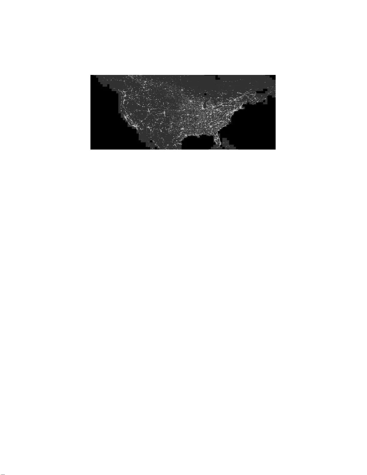
Comments & Academic Discussion
Loading comments...
Leave a Comment