A Bayesian encourages dropout

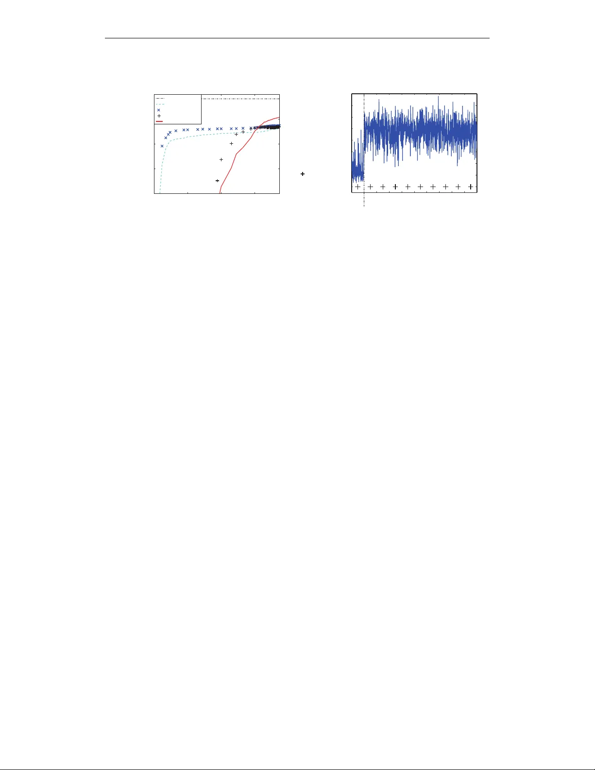
Under revie w as a conference paper at ICLR 2015 A B A Y E S I A N E N C O U R A G E S D R O P O U T Shin-ichi Maeda Graduate School of Informatics Kyoto Uni versity Y oshidahonmachi 36-1, Sakyo, K yoto, Japan ichi@sys.i.kyoto-u.ac.jp A B S T R A C T Dropout is one of the ke y techniques to prevent the learning from o verfitting. It is explained that dropout works as a kind of modified L2 regularization. Here, we shed light on the dropout from Bayesian standpoint. Bayesian interpretation enables us to optimize the dropout rate, which is beneficial for learning of weight parameters and prediction after learning. The experiment result also encourages the optimization of the dropout. 1 I N T RO D U C T I O N Recently , large scale neural networks has successfully shown its great learning abilities for various kind of tasks such as image recoginition, speech recognition or natural language processing. Al- though it is likely that the lar ge scale neural networks fail to learn the appropriate parameter because of its huge model complexity , the dev elopment of sev eral learning techniques, optimization and utilization of large dataset o vercome such difficulty of learning. One such successful learning technique is ‘dropout’, which is considered to be important to suppress the o verfitting (Hinton et al., 2012). The success of dropout attracts many researchers’ attention and sev eral theoretical studies hav e been performed aiming for better understanding of dropout (W ager et al., 2013; Baldi & Sado wski, 2013; Ba & Frey, 2013). The most of them explain the dropout as a kind of new input in variant regularization technique, and prove the applicability to other applications such as generalized linear model (W ager et al., 2013; W ang & Manning, 2013). In contrast, we formally provide a Bayesian interpretation to dropout. From this standpoint, we can think that the dropout is a way to solve the model selection problem such as input feature selec- tion or the selection of number of hidden internal states by Bayesian averaging of the model. That is, the inference after dropout training can be considered as an approximate inference by Bayesian model av eraging where each model is weighted in accordance with the posterior distribution, and the dropout training can be considered as an approximate learning of parameter which optimizes a weighted sum of likelihoods of all possible models, i.e., marginal likelihood. This interpreta- tion enables the optimization of ‘dropout rate’ as the learning of the optimal weights of the model, i.e., posterior of the model. This optimization of dropout rate benefits the parameter learning by a better approximation of marginal likelihood and prediction by a closer distribution to the predic- tiv e distribution. Note the Bayesian vie w on ‘dropout’ was already seen in the original paper of dropout (Hinton et al., 2012) which regards the dropout training as a kind of approximate Bayesian learning, howe ver it was not mentioned how much the gap would be between the dropout training and standard Bayesian learning, and how to set or optimize the dropout rate. 2 S T A N D A R D D R O P O U T A L G O R I T H M 2 . 1 D R O P O U T T R A I N I N G W e will explain the dropout for three-layered neural network not only because the neural network is the first model that the dropout training is applied, but also because it is one of the simplest models that in volves both of the input feature selection problem and the hidden internal units selection problem. Note the concept of dropout itself can be easily extended to an y other learning machines. 1 Under revie w as a conference paper at ICLR 2015 Let x ∈ < n , h ∈ < m , and y ∈ < l be n -dimensional input, m -dimensional hidden unit, and l - dimensional output, respectively . Then, the hidden unit h and the output y are computed as follo ws;  h = σ ( W (1) x + b (1) ) , y = σ ( W (2) h + b (2) ) , where W (1) and W (2) are m × n and l × m matrix, and b (1) and b (2) are m - and l -dimensional vector , respectiv ely . σ ( · ) is a nonlinear acti vation function such as a sigmoid function. The set θ = { W (1) , W (2) , b (1) , b (2) } is a parameter set to be optimized. Now we consider the model selection problem where the full model is represented as the one de- scribed abov e, and the other possible models (submodels) consist of the subset of the input features or the hidden units of the full model. Let us introduce the diagonal mask matrices Z (1) and Z (2) where the i -th diagonal elements z (1) i ∈ { 0 , 1 } ( i = 1 , · · · , n ) and z (2) j ∈ { 0 , 1 } ( j = 1 , · · · , m ) are both binary to represent such subsets. W e will sometimes use z = { z (1) i , z (2) j | i = 1 , · · · , n, j = 1 , · · · , m } to represent all the mask variables. Then the possible model is represented as follows;  h = σ ( W (1) Z (1) x + b (1) ) , y = σ ( W (2) Z (2) h + b (2) ) . The determination of Z (1) corresponds to the input feature selection problem while the determina- tion of Z (2) corresponds to the hidden internal units selection problem. W e may rewrite y ( x ; θ ) with y ( x ; Z (1) , Z (2) , θ ) to represent the explicit dependence on the masks Z (1) and Z (2) as well as the parameter θ . There are 2 ( m + n ) possible architectures when ignoring the redundancy brought by the hierarchy of the architecture, and this number becomes huge in practice. This poses a great challenge in the optimization of the best mask z , i.e., the best model selection. Instead of choosing a specific binary mask z , the standard dropout takes the approach to stochas- tically mix all the possible models by a stochastic optimization. The algorithm is summarized as follows; Standard dropout for learning : 1. Set t = 0 and set an initial estimate for parameter θ 0 . 2. Pick a pair of sample ( x t , y t ) at random. 3. Randomly set the mask z t by determining e very element independently according to the dropout rate, typically , Ber(0 . 5) where Ber(p) denotes a Bernoulli distribution with prob- ability p . 4. Update the parameter θ as θ t +1 = θ t + η t ∂ log p ( y t | x t , z t , θ ) ∂ θ , where η t determines a step size, and should be decreased properly to assure the con- ver gence. In case of the training of the three-layered neural network for regression, log p ( y t | x t , z t , θ ) ∝ −|| y t − y ( x t ; Z (1) t , Z (2) t , θ ) || 2 2 where || · || 2 denotes a Euclidean norm. 5. Increment t and go to step 2 unless certain termination condition is not satisfied. 2 . 2 P R E D I C T I O N A F T E R D RO P O U T T R A I N I N G After training of θ , the output for the test input x ∗ is giv en as E p ( Z (1) ) p ( Z (2) ) h y ( x ∗ ; Z (1) , Z (2) , θ ) i ≈ y  x ∗ ; E p ( Z (1) ) [ Z (1) ] , E p ( Z (2) ) [ Z (2) ] , θ  , (1) where E p ( z ) [ f ( z )] denotes an expected value of function f ( z ) with respect to the distribution p ( z ) . The distribution p ( Z (1) ) and p ( Z (2) ) in this case must correspond to the ones used in choosing mask matrices Z (1) and Z (2) during learning. If an independent Bernoulli distirbution with prob- ability p = 0 . 5 is used for both choosing Z (1) and Z (2) , then the three-layered neural network 2 Under revie w as a conference paper at ICLR 2015 output y  x ∗ ; E p ( Z (1) ) [ Z (1) ] , E p ( Z (2) ) [ Z (2) ] , W (1) , W (2) , b (1) , b (2)  is equiv alent to the output us- ing halved weights y  x ∗ ; 1 2 W (1) , 1 2 W (2) , b (1) , b (2)  . There is another way to approximate E p ( Z (1) ) p ( Z (2) )  y ( x ∗ ; Z (1) , Z (2) , θ )  known as ‘fast dropout’ (W ang & Manning, 2013). When we apply dropout, not only to neural network, b ut also to other models, we often need to compute a weighted sum of many independent random variables w T Z x where the upper script T denotes a transpose of vector (or matrix), w is a weight vector , and Z is a diagonal mask matrix whose diagonal elements are binary random v ariables. x is either a sample of the input or the hidden unit, and treated as a fixed value. Fast dropout approximates this weighted sum of random variables by a single Gaussian random v ariable utilizing L yapunov’ s central limit theorem. This Gaussianization improves the accuracy of the calculation of the expectation while saving the computation time. It is also shown that the Gaussian approximation is beneficial to the learning. 3 E X I S T I N G I N T E R P R E T A T I O N S O F D RO P O U T A L G O R I T H M Although the idea of dropout originates from Bayesian model a veraging, it is proposed that the arti- ficial corruption of the model by dropout is interpreted as a kind of adaptiv e regularization (W ager et al., 2013; W ang & Manning, 2013) analogous with the artificial feature corruption that is inter- preted as a kind of regularization. Under this viewpoint, the dropout regularizer used for generalized linear model can be seen as the first-order equiv alent to L 2 -regularization after transforming the in- put by an estimate of the in verse diagonal Fisher information matrix (W ager et al., 2013). This input transformation let the regularizer scale in variant while the con ventional L 2 -regularizer does not hold this desirable property . In (Baldi & Sadowski, 2013), the cost function used in dropout training is analyzed. The cost function used in dropout training is considered as an av erage of the cost function of submodels. They analyze the difference of the average of the cost function of submodels and a cost function of the av erage of the submodels, and show that the dropout brings an input-dependent regularization term to the cost function of the average of the submodels. They also pointed out that the strongest regularization ef fect is obtained when the dropout rate is set to be 0.5, which is a typical value used in practice. There is also a study that treats dropout from Bayesian vie wpoint. Ba & Frey (2013) extend the dropout to ‘standout’ where the dropout rate is adapti vely trained. The y propose that the random masks used in dropout training should be considered as a random v ariable of the Bayesian posterior distribution over submodels, which shares our view to the dropout. Howe ver , their proposed adaptiv e dropout rate depends on each input v ariable, which implies there should be a different mask for each input, while here we assume a consistent mask for whole dataset, and tries to estimate the best mix of models based on the entire training dataset. Also, it is not clear wh y their update of the dropout rate works as the leaning of the posterior . In the following section, we will show a clear interpretation of dropout from Bayesian standpoint, and provide a theoretically solid way to optimize the dropout rate. The difference of our study from the e xisting studies will be further discussed in Section 7. 4 B AY E S I A N I N T E R P R E T A T I O N O F D R O P O U T A L G O R I T H M 4 . 1 B AY E S I A N I N T E R P R E TA T I O N O F D RO P O U T T R A I N I N G In standard Bayesian framew ork, all the parameters are treated as random variables to be inferred via posterior except for the hyper parameter . In dropout training, θ in Section 2 corresponds to the hyper parameter while the mask z in Section 2 corresponds to the parameter . Let us denote z an m -dimensional binary mask vector whose elements take either 0 or 1 , D = { x 1 , y 1 , · · · , x T , y T } the set of training data set. Then the marginal log-lik elihood for hyperparameter θ is defined as log p ( D | θ ) ≡ log X z  Y T t =1 p ( y t | x t , z , θ )  p ( z ) . 3 Under revie w as a conference paper at ICLR 2015 Although we omit the dependence of θ on p ( z ) here for simplicity , it is possible to include such dependence in general. By introducing any distribution of the parameter z , q ( z ) , which we call trial distribution follo wing the con ventions, the marginal log-lik elihood can be written as log p ( D | θ ) = E q ( z ) [log p ( D | θ )] = E q ( z )  log p ( D , z | θ ) p ( z | D , θ )  = E q ( z ) [log p ( D , z | θ )] − E q ( z ) [log q ( z )] + K L [ q ( z ) | p ( z | D , θ )] ≥ E q ( z ) [log p ( D , z | θ )] − E q ( z ) [log q ( z )] = X T t =1 X z q ( z ) log p ( y t | x t , z , θ ) + X z q ( z ) log p ( z ) − X z q ( z ) log q ( z ) ≡ F ( q ( z ) , θ ) , (2) where K L [ q ( z ) | p ( z )] ≡ P z q ( z ) log q ( z ) p ( z ) denotes a Kullback-Leibler div ergence between the dis- tritbuions q ( z ) and p ( z ) , and p ( z | D, θ ) ∝ P z  Q T t =1 p ( y t | x t , z , θ )  p ( z ) is a posterior distribution. The lower bound in Eq. (2) is valid for any trial distribution q ( z ) because of the non-negati vity of Kullback-Leibler diver gence, and becomes tight only when the trial distribution q ( z ) corresponds to the posterior p ( z | D , θ ) . This means q ( z ) should be close to the posterior p ( z | D , θ ) to minimize the gap. Because θ depends only on the first term of Eq. (2), the maximization of the marginal likelihood with respect to θ for some fixed q ( z ) is equiv alent to the maximization of the first term of Eq. (2), i.e., θ ∗ = arg max θ F ( q ( z ) , θ ) = arg max θ X t X z q ( z ) log p ( y t | x t , z , θ ) , (3) The above optimization of the lower bound by the stochastic gradient descent leads the dropout training algorithm e xplained in Section 2. Note that we need to randomly sample both the input- output pair { x t , y t } and the mask z . The sample of the mask v ariable z should obey the trial distribution q ( z ) . T o be identical to the dropout training explained in Section 2.1, we need to assume p ( z ) = Q m i =1 p z i (1 − p ) z i and q ( z ) = p ( z ) . In this case, the parameter p corresponds to the dropout rate. In this paper , we will say q ( z ) as the dropout rate because q ( z ) determines the dropout rate. 4 . 2 B AY E S I A N I N T E R P R E TA T I O N O F T H E P R E D I C T I O N A F T E R D RO P O U T T R A I N I N G W e can also interpret the output for the test input x ∗ after learning of θ from a Bayesian standpoint. In a Bayesian framew ork, the output for the test input x ∗ should be inferred as the expected v alue of the predictiv e distribution gi ven as Z y p ( y | x ∗ , D , θ ) d y = X z Z y p ( y | x ∗ , z , θ ) d y p ( z | D , θ ) , (4) That is, the output is predicted by the weighted average of submodel predictions R y p ( y | x ∗ , z , θ ) d y . Howe ver , the abov e calculation becomes often intractable since the exact calculation of both the posterior itself and the expectation with respect to the posterior needs the summation over z which has 2 m variations. Therefore, consider to replace the posterior p ( z | D , θ ) with some tractable trial distribution q ( z ) . Z y p ( y | x ∗ , D , θ ) d y ≈ X z Z y p ( y | x ∗ , z , θ ) d y q ( z ) ≈ Z y p ( y | x ∗ , E q ( z ) [ z ] , θ ) d y , (5) When we use independent p ( z ) for q ( z ) , we will ha ve the same output explained in Section 2.2. The last approximation in Eq.(5) is the approximation to the e xpectation o ver q ( z ) . This may be replaced by a Gaussian approximation explained in Section 2.2. 5 B AY E S I A N D R O P O U T A L G O R I T H M W I T H V A R I A B L E D RO P O U T R A T E As apparent from the discussion in the preceding section, q ( z ) should be close to the posterior p ( z | D , θ ) because it makes the lower bound much more tight, which means the cost function 4 Under revie w as a conference paper at ICLR 2015 F ( q ( z ) , θ ) with respect to θ is presumably closer to the desirable cost function, marginal log- likelihood log p ( D | θ ) . Moreover , it enables to approximate the predictiv e distribution much more accurately when we use q ( z ) that better approximates the posterior p ( z | D , θ ) . The best q ( z ) is the posterior p ( z | D , θ ) which, howe ver , cannot be solved in an analytical form in most cases. So consider to optimize q ( z ) in a certain parametric distribution family , q ( z | λ ) that is parameterized by λ . Then the best parameter λ ∗ is obtained as the one that maximizes the lower bound, λ ∗ = arg min λ K L [ q ( z | λ ) | p ( z , D , θ )] = arg max λ F ( q ( z | λ ) , θ ) . (6) The above optimization problem could be solved by a numerical optimization method such as a stochastic gradient descent. Overall, the entire Bayesian dropout algorithm would be as follo ws; Bayesian dropout for learning : 1. Set t = 0 and set an initial estimate for parameters θ 0 and λ 0 . 2. Pick a pair of sample ( x t , y t ) at random. 3. Randomly set a mask z t by determining every element independently according to the dropout rate q ( z | λ t ) . 4. Update the parameter θ as θ t +1 = θ t + η t ∂ log p ( y t | x t , z t , θ ) ∂ θ . 5. Update the parameter of the dropout rate q ( z | λ t ) as λ t +1 = λ t +  t  ∂ log q ( z t | λ ) ∂ λ log p ( y t | x t , z t , θ ) + δ t ∂ ∂ λ  X z q ( z | λ ) log p ( z ) − X z q ( z | λ ) log q ( z | λ )   , (7) where η t and  t determine step sizes, and should be decreased properly to assure the con- ver gence while δ t is an inv erse of the effecti ve number of samples, which will be explained later . 6. Increment t and go to step 2 unless certain termination condition is not satisfied. The first term in the right hand side of Eq. (7) comes from the first term of the deriv ativ e of F ( q ( z | λ ) , θ ) /T , ∂ ∂ λ 1 T P T t =1 P z q ( z ) log p ( y t | x t , z , θ ) ≈ E q ( z | λ ) h E r ( x , y ) h ∂ log q ( z | λ ) ∂ λ log p ( y | x , z , θ ) ii where E q ( z | λ ) [ · ] and E r ( x , y ) [ · ] denote the ex- pectation with respect to the trial distribution q ( z | λ ) and the true distribution of the training set { x t , y t | t = 1 , · · · , T } . Because these two expectations cannot be e valuated analytically in most cases due to the complex dependence of log p ( y | x , z , θ ) on both { x , y } and z , the expectations are replaced by random samples according to the recipe of the stochastic gradient descent. In contrast, the rest of two terms corresponding to the deriv ativ es of the last two terms of F ( q ( z | λ ) , θ ) /T can be ev aluated directly if we assume independent distributions for both p ( z ) = Q m i =1 p ( z i ) and q ( z ) = Q m i =1 q ( z i | λ ) . The summation ov er z is usually intractable because z has 2 m variations. Howe ver , the independence assumption decomposes the intractable summation ov er z into m tractable summations over a binary z i ( i = 1 , · · · , m ) . This allo ws us the direct ev aluation of these terms in practice without using Monte Carlo method. That is the reason why the last tw o terms does not depend on the sample z t as well as { x t , y t } . A scalar δ t denotes an in verse of the ef fective number of samples, i.e., δ t ∝ 1 /T so that the last tw o terms correspond to the deriv ative of the last two terms of F ( q ( z | λ ) , θ ) /T . This may be scheduled as δ t ∝ 1 /t when we think the amount of the training data is increasing as the algorithm proceeds. 5 Under revie w as a conference paper at ICLR 2015 It is noted that many other variants of this algorithm can be considered. For example, we can introduce momentum term, we can update the parameters for a mini-batch, or we can consider EM- like algorithm, i.e., the update of θ (steps 2-4) is repeatedly performed until ∂ F ( q ( z | λ ) ,θ ) ∂ θ ≈ 0 holds, then proceeds to the update of λ , and λ is updated until ∂ F ( q ( z | λ ) ,θ ) ∂ λ ≈ 0 holds. Follo wing the standard dropout training, one natural choice of the parameterization of q ( z | λ ) would be q ( z | λ ) = Q m i =1 λ z i (1 − λ ) (1 − z i ) where λ represents a common dropout rate to all the input features. Hereafter , we will refer the dropout with the optimized uniform scalar λ to uniformly optimized rate dropout (UOR dropout). W e could consider other parameterizations of q ( z | λ ) . For example, we can parameterize for each q ( z i = 1) differently by letting q ( z i = 1) = λ i . Hereafter , we will refer the dropout with the optimized element-wise λ i to feature-wise optimized rate dropout (FOR dropout). The parameter of the mask distribution can specify the distribution of subset of z independently , such as, q ( z j = 1) = λ i (if z j ∈ I i ) where I i denotes i -th subset of z . The subset could be the units in a same layer . This layer-wise setting of the dropout rate is sometimes used in practice, e.g., (Graham, 2014). 6 E X P E R I M E N T W e test the v alidity of the optimization of the dropout rate with a binary classification problem. 6 . 1 D A TA Let y ∈ { 0 , 1 } be a target binary label and x be a 1000-dimensional input vector consisting of 100- dimensional informati ve features and the rest of 900-dimensional non-informati ve features. Label y obeys Ber(0 . 5) . Each informati ve feature x i ( i = 1 , · · · , 100 ) is generated independently according to p ( x i | y = 0) = N ( x i | − 0 . 1 , 1) and p ( x i | y = 1) = N ( x i | 0 . 1 , 1) so that each informativ e feature has a weak correlation with the label y (cross-correlation is 0.1) while each non-informativ e feature x i ( i = 101 , · · · , 1000 ) is generated independently according to p ( x i ) = N ( x i | 0 , 1) irrelev ant to the label y . Here, N ( x | µ, s 2 ) denotes a Gaussian distribution with mean µ and variance s 2 . 2000 samples are generated for the training, and another 1000 samples are generated for the validation. The performance is ev aluated with another 20,000 test samples. 6 . 2 M O D E L A N D A L G O R I T H M Linear logistic regression is used for this task. p ( y = 1 | x , z , θ ) = 1 1 + exp( − θ T Z x ) ≡ σ ( θ T Z x ) , (8) where Z is a diagonal matrix whose diagonal elements are binary masks z . In this case, the Gaussian approximation to θ T Z x works effecti vely as proposed in (W ang & Manning, 2013). Approximating u = θ T Z x by a Gaussian random variable whose mean is µ = P m i =1 q ( z i = 1) θ i x i and whose vari- ance is s 2 = q ( z i = 0) q ( z i = 1)( θ i x i ) 2 , and applying a well-known formula which approximates Gaussian integral of sigmoid function σ ( x ) , the predictive distrib ution is obtained as p ( y = 1 | x , θ ) ≈ Z σ ( u ) N ( u | µ, s 2 ) du ≈ σ µ p 1 + π s 2 / 8 ! . (9) W e compared four algorithms, 1) maximum likelihood estimation (MLE), 2) standard dropout algo- rithm (fixed dropout) where the dropout rate is fixed to be 0.5, 3) Bayesian dropout algorithm that optimizes a uniform dropout rate (UOR dropout), and 4) Bayesian dropout algorithm that optimizes feature-wise dropout rates (DOR dropout). For the optimization of θ and λ , we need to determine the step sizes η t and  t of the algorithm described in Section 5 properly . These values are sched- uled as η t = a 1+ t/b and  t = c 1+ t/d . The step size  t used for updating λ should be decreased slower than η used for updating θ . Considering this, we chose the best parameter set a, b, c , and d that shows the best accuracy for the validation data among a ∈ { 3 · 10 − 4 , 10 − 3 , 3 · 10 − 2 , 10 − 2 } , b ∈ { 10 2 , 10 3 , 10 4 } , c ∈ { 3 · 10 − 4 , 10 − 3 , 3 · 10 − 2 , 10 − 2 } , d ∈ { 10 3 , 10 4 , 10 5 } , respectiv ely . For Bayesian dropout algorithm, the in verse of the ef fective number of samples δ is simply set to be the 6 Under revie w as a conference paper at ICLR 2015 0.65 0.7 0.75 0.8 MLE xed dropout UOR dropout FOR dropout Bayes optimal 100 0 0.2 0.4 0.6 0.8 1000 inputfeatureindex Trained featurewise dropoutrate accuracy (b) (a) #ofupdates 10 10 10 10 0 2 4 6 informative features non-informative features uniform dropout rate () Figure 1: Experimental results (a) T est accuracy (b) Dropout rate after learning in verse of the number of samples, i.e., 10 − 3 , and the initial value of the dropout rate is set to be all 0.5 for both UOR dropout and DOR dropout. 6 . 3 R E S U LT T est accuracy after learning is sho wn in Fig.1(a), and the trained dropout rate is shown in Fig.1(b). In Fig.1(b), the height of the bar denotes the dropout rate of FOR dropout while ’+’ denotes the dropout rate of UOR dropout. Because only 10 % of features are rele vant to the input, it is difficult to determine the best uniform dropout rate. Eventually , the optimized uniform dropout rate becomes zero. Then, the test accura- cies of both MLE and UOR dropout takes almost same value. Fixed dropout rate shows a slightly better accuracy although the difference cannot be visible from Fig. 1(a). On the other hand, if we op- timize the feature-wise dropout rate, the test accuracy increases, getting closer to the Bayes optimal (theoretical limit). As can be seen from Fig1.(b), only the dropout rate of the informative features (the first 100 elements) are selectiv ely lo w . Note that FOR dropout sho ws a significant regularization effect although it has no h yperparameter to be tuned. 7 D I S C U S S I O N 7 . 1 W H Y B A Y E S I A N ? The input feature selection problem and the hidden internal units selection problem is, in general, difficult because it requires to compare a v ast number of models as large as 2 n and 2 m in case of the three-layered neural network explained in Section 2. Moreov er, the maximum likelihood criterion is not useful in choosing the best mask z because it always prefers the largest network, that is, it always chooses z = 1 where 1 is a vector containing all 1 in its elements. max z ,θ X t log p ( y t | x t , z , θ ) = max θ X t log p ( y t | x t , z = 1 , θ ) . (10) It is a well kno wn fact that the number of the parameters has a proportional relation with the discrep- ancy between the generalization error and the training error of the non-singular statistical models trained by Maximum a Posteriori (MAP) estimation which uses a fixed prior and the maximum likelihood estimation (see Section 6.4 of W atanabe (2009) for example). In contrast, Bayesian inference does not rely on the prediction of a single model, but on the weighted sum of submodel predictions where the weights are determined according to the posterior of the submodel.The marginal likelihood integrated over all possible submodels can take into account the complexity of the model. This fact helps to prev ent the overfitting of the type explained in Section 3.4 of (Bishop, 2006). As for the asymptotic behavior of the Bayes generalization error, there are studies from algebraic geometry (W atanabe, 2009), which rev eal that the asymptotic behavior of a 7 Under revie w as a conference paper at ICLR 2015 singular statistical model is dif ferent from that of the non-singular statistical model; The generaliza- tion error does not increase necessary proportionally to the number of the parameters. This partly explains the reason why the recent big neural network, which is categorized into a singular statistical model, can resist overfitting as opposed to the regular statistical model optimized by the maximum likelihood estimation or MAP estimation. 7 . 2 W H A T ’ S D I FF E R E N T F RO M T H E O T H E R S T U D I E S ? There are sev eral studies that vie w dropout training as a kind of approximate Bayesian learning except for the original study (Hinton et al., 2012). Ho wev er, their interpretation differ from our interpretation or lacks solid theoretical foundation. In (W ang & Manning, 2013), it is stated that the cost function for θ can be seen as the lower bound of the marginal log-likelihood. Howe ver , their marginal log-likelihood is de- fined as log[ E p ( z ) p ( y | θ T Z x )] which has a lo wer bound E p ( z ) [log p ( y | θ T Z x )] with an inde- pendent Bernoulli distribution p ( z ) as the dropout rate. Similar cost function is proposed by (Ba & Frey, 2013). They propose to optimize the dropout rate q ( z | x , λ ) so as to maximize E q ( z | x ,λ ) [log p ( y | θ T Z x )] . Basically , their view on z is a hidden v ariable rather than a parameter be- cause z is not inferred by the entire training dataset, but inferred sample by sample as p ( z t | x t , y t ) . In contrast, we define the marginal likelihood as log p ( D | θ ) ≡ log P z  Q T t =1 p ( y t | x t , z , θ )  p ( z ) . W ith this definition, we may interpret the computation of the expectation of the submodel prediction with respect to the submodel posterior p ( z | D, θ ) (i.e. Bayesian model averaging) as a Bayesian way to solve the model selection problem. W e shall note that, in the context of the neural network, there is nothing new about the philosophy of assigning the prior to the parameter θ and seeking the posterior achieving the best Bayesian prediction Eq. (4). See, for example, (Neal, 1996; Xiong et al., 2011), which assigned Gaussian distribution to the weight matrices W s. The search of the optimal prior ov er the vast space of probability measures is indeed a daunting task, ho wever . The aforementioned algorithms do suffer from runtime. From this computational point of vie w , the standard dropout algorithm emerges as an efficient Bayesian compromise to this search. In particular , it restricts the search of the distribution of each ( i, j ) element of W , W ij to the ones for which one can write as W ij = z j ˜ W ij z j ∼ Ber(0 . 5) iid, ˜ W ij deterministic for all j -th unit adjacent to the connection ( i, j ) 1 . In other words, the algorithm only looks into a specific family of discrete valued distributions parametrized by the v alues of ˜ W ij . This way , the standard dropout algorithm bridges between the stochastic feature selection and the Beyesian av eraging. In this light, our algorithm can be seen as one step improv ement of the standard dropout algorithm, which restricts the search of the posterior distribution of W ij to the ones of the form W ij = z j ˜ W ij z j ∼ Ber( p j ) iid, ˜ W ij deterministic for all j -th unit adjacent to the connection ( i, j ) . This is a set of discrete v alued distributions parametrized by ˜ W ij and p j . Because the search space becomes larger , our method will consume more runtime than the standard dropout algorithm. By allowing more freedom to the distribution, howe ver , one can expect the trained machine to be much more data specific. As apparent from the abov e discussion, we can consider the dropconnect (W an et al., 2013) as another parameterization of the distribution of W ij , i.e., W ij = z ij ˜ W ij where z ij obeys a Bernoulli distrib ution. If need be, one can also group p j s to match the specific task required for the model. For e xample, let us consider the family of time-series prediction model such as vector autore gression (V AR) model: X t = M X k =1 A k X t − k X ∈ R d . 1 T o precisely correspond to the original dropout algorithm, we also need to set the prior p ( z ) appropriately so that the re guralization term P z q ( z ) log p ( z ) − P z q ( z ) log q ( z ) becomes identical with the re guralization term used in the original dropout aglorithm. 8 Under revie w as a conference paper at ICLR 2015 For this family , the number of parameters will gro w quickly with the state space dimension d and the size of lag time M , making the search for the best posterior distribution difficult. Again, we may put A k ∼ Z ( k ) ˜ A k where Z ( k ) are diagonal matrices with entries { Ber( p ( k ) i ) i = 1 , · · · , d } . W e may reduce the number of the hyperparameters by assuming some structure to the set of p ( k ) i s; for example, we can put p ( k ) i = ˜ p k or p ( k ) i = ˜ p k λ i and introduce an intended space-time correlations. This type of parametrization may allow us to resolve a v ery sophisticated feature selection problems, which are considered intractable by the con ventional methods. R E F E R E N C E S Ba, Jimmy and Frey , Brendan. Adapti ve dropout for training deep neural networks. In Advances in Neural Information Pr ocessing Systems , pp. 3084–3092, 2013. Baldi, Pierre and Sadowski, Peter J. Understanding dropout. In Advances in Neural Information Pr ocessing Systems , pp. 2814–2822, 2013. Bishop, Christopher M. P attern r ecognition and machine learning , volume 1. springer Ne w Y ork, 2006. Graham, Benjamin. Spatially-sparse conv olutional neural networks. arXiv preprint arXiv:1409.6070 , 2014. Hinton, Geoffre y E, Sriv astava, Nitish, Krizhe vsky , Alex, Sutskev er, Ilya, and Salakhutdinov , Rus- lan R. Improving neural networks by prev enting co-adaptation of feature detectors. arXiv pr eprint arXiv:1207.0580 , 2012. Neal, Radford M. Bayesian learning for neural networks . Springer-V erlag Ne w Y ork, Inc., 1996. W ager , Stefan, W ang, Sida, and Liang, Percy . Dropout training as adapti ve regularization. In Advances in Neural Information Pr ocessing Systems , pp. 351–359, 2013. W an, Li, Zeiler , Matthe w , Zhang, Sixin, Cun, Y ann L, and Fergus, Rob. Regularization of neural networks using dropconnect. In Pr oceedings of the 30th International Confer ence on Machine Learning (ICML-13) , pp. 1058–1066, 2013. W ang, Sida and Manning, Christopher . Fast dropout training. In Proceedings of the 30th Interna- tional Confer ence on Machine Learning (ICML-13) , pp. 118–126, 2013. W atanabe, Sumio. Algebraic geometry and statistical learning theory , volume 25. Cambridge Univ ersity Press, 2009. Xiong, Hui Y uan, Barash, Y oseph, and Frey , Brendan J. Bayesian prediction of tissue-regulated splicing using RN A sequence and cellular context. Bioinformatics , 27(18):2554–2562, 2011. 9