Robust Topological Inference: Distance To a Measure and Kernel Distance

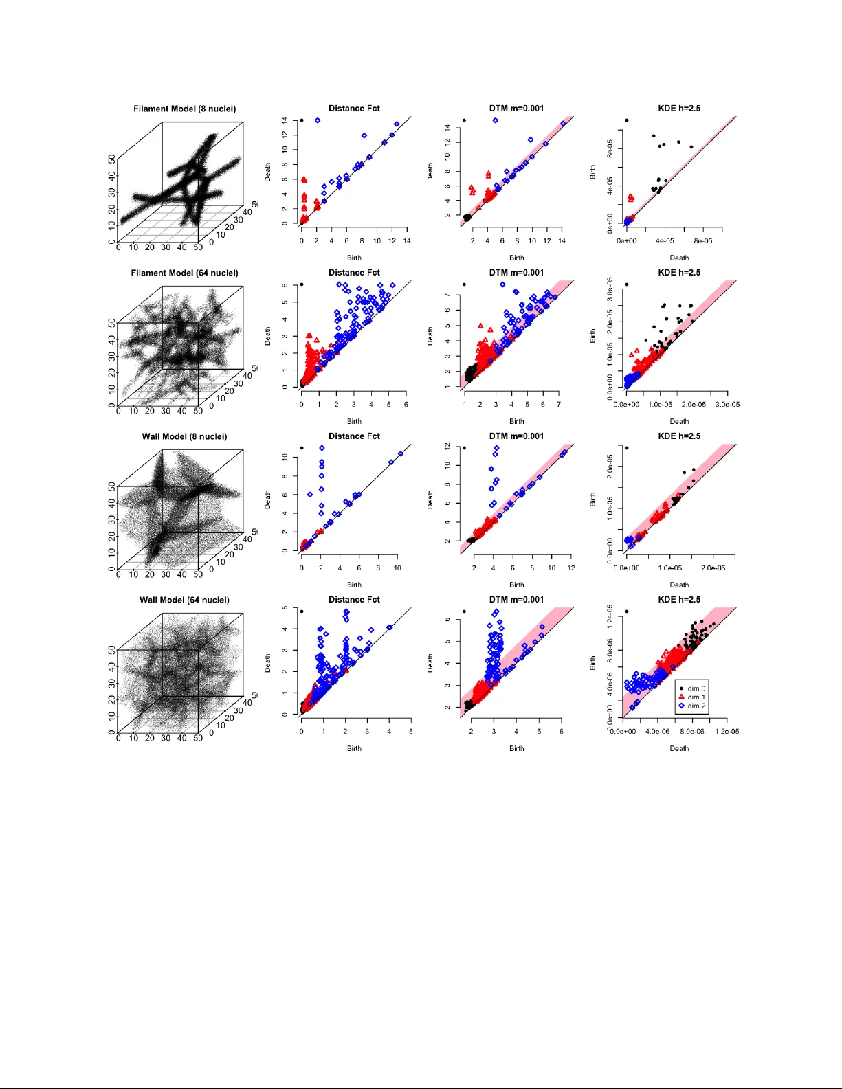
Submitted to the Annals of Statistics ROBUST TOPOLOGICAL INFERENCE: DIST ANCE TO A MEASURE AND KERNEL DIST ANCE B Y F R É D É R I C C H A Z A L 1 , ∗ , B R I T T A N Y T E R E S E F A S Y 2 , F A B R I Z I O L E C C I 3 , † , B E R T R A N D M I C H E L 4 , ∗ , A L E S S A N D R O R I N A L D O 3 , † , A N D L A R R Y W A S S E R M A N 3 , ‡ , 1 INRIA 2 T ulane University 3 Carnegie Mellon University 4 Université Pierre et Marie Curie December 24, 2014 Let P be a distribution with support S . The salient features of S can be quantified with persistent homology , which summarizes topolog- ical features of the sublevel sets of the distance function (the distance of any point x to S ). Given a sample from P we can infer the persistent homology using an empirical version of the distance function. However , the empirical distance function is highly non-robust to noise and out- liers. Even one outlier is deadly . The distance-to-a-measure (DTM), in- troduced by Chazal et al. ( 2011 ), and the kernel distance , introduced by Phillips et al. ( 2014 ), are smooth functions that provide useful topologi- cal information but are robust to noise and outliers . Chazal et al. ( 2014 ) derived concentration bounds for DTM. Building on these results, we de- rive limiting distributions and confidence sets , and we propose a method for choosing tuning parameters . 1. Introduction. Figure 1 shows three complex point clouds , based on a model used for simu- lating cosmology data. V isually , the three samples look very similar . Below the data plots are the persistence diagrams, which are summaries of topological features defined in Section 2. The persis- tence diagrams make it clearer that the third data set is from a different data generating process than the first two. This is an example of how topological features can summarize structure in point clouds. The field of topological data analysis (TDA) is concerned with defining such topological features; see Carlsson ( 2009 ). When performing TDA, it is important to use topological measures that are robust to noise. This paper explores some of these robust topological measures . Let P be a distribution with compact support S ⊂ R d . One way to describe the shape of S is by using homology . Roughly speaking, the homology of S measures the topological features of S , such as the connected components, the holes, and the voids. A more nuanced way to describe the shape of S is using persistent homology , which is a multiscale version of homology . T o describe persistent homology , we begin with the distance function ∆ S : R d → R for S which is defined by (1) ∆ S ( x ) = inf y ∈ S k x − y k . The sublevel sets L t = { x : ∆ S ( x ) ≤ t } provide multiscale topological information about S . As t varies from zero to ∞ , topological features — connected components, loops, voids — are born and die. P er- ∗ Research supported by ANR-13-BS01-0008. † Research supported by NSF CAREER Grant DMS 1149677. ‡ Research supported by Air F orce Grant F A95500910373, NSF Grant DMS-0806009. Keywords and phrases: persistent homology, topology, density estimation. 1 sistent homology quantifies the evolution of these topological features as a function of t . See Figure 2 . Each point on the persistence diagram represents the birth and death time of a topological feature . Given a sample X 1 , . . . , X n ∼ P , the empirical distance function is defined by (2) b ∆ ( x ) = min X i k x − X i k . If P is supported on S , and has a density bounded a wa y from zero and infinity , then b ∆ is a consistent estimator of ∆ S , i.e., sup x | b ∆ ( x ) − ∆ S ( x ) | P → 0. However , if there are outliers, or noise, then b ∆ ( x ) is no longer consistent. Figure 3 (bottom) shows that a few outliers completely change the distance func- tion. In the language of robust statistics , the empirical distance function has breakdown point zero. A more robust approach is to estimate the persistent homology of the super -level sets of the density p of P . As long as P is concentrated near S , we expect the level sets of p to provide useful topological information about S . Specifically , some level sets of p are homotopic to S under weak conditions , and this implies that we can estimate the homology of S . Note that, in this case, we are using the persistent homology of the super-level sets of p , to estimate the homology of S . This is the approach suggested by Bubenik ( 2012 ), F asy et al. ( 2014b ) and Bobrowski et al. ( 2014 ). A related idea is to use persistent homology based on a kernel distance ( Phillips et al. , 2014 ). In fact, the sublevel sets of the kernel distance are a rescaling of the super -level sets of p , so these two ideas are essentially equivalent. W e discuss this approach in Section 5 . A different approach, more closely related to the distance function, but robust to noise, is to use the distance-to-a-measure (DTM) , δ ≡ δ P , m , from Chazal et al. ( 2011 ); see Section 2 . An estimate b δ of δ is obtained by replacing the true probability measure with the empirical probability measure P n , or with a deconvolved version of the observed measure Caillerie et al. ( 2011 ). One then constructs a persistence diagram based on the sub-level sets of the DTM. See Figure 1 . This approach is aimed at estimating the persistent homology of S . (The DTM also suggests new approaches to density estimation; see Biau et al. ( 2011 ).) The density estimation approach and the DTM are both trying to probe the topology of S . But the former is using persistent homology to estimate the homology of S , while the DTM is directly trying to estimate the persistent homology of S . W e discuss this point in detail in Section 9.1 . In this paper , we explore some statistical properties of these methods . In particular: 1. W e show that p n ( b δ 2 ( x ) − δ 2 ( x )) converges to a Gaussian process. (Theorem 5 ). 2. W e show that the bootstrap provides asymptotically valid confidence bands for δ . This allows us to identify significant topological features . (Theorem 18 ). 3. W e find the limiting distribution of a key topological quantity called the bottleneck distance. (Section 4.1 ). 4. W e also show that, under additional assumptions, there is another version of the bootstrap — which we call the bottleneck bootstrap — that provides more precise inferences . (Section 6 ). 5. W e show similar results for the kernel distance. (Section 5 ). 6. W e propose a method for choosing the tuning parameter m for DTM and the bandwidth h for the kernel distance. (Section 7.1 ). 7. W e show that the DTM and the KDE both suffer from boundary bias and we suggest a method for reducing the bias . (Section 7.2 ). Notation. B ( x , ² ) is a Euclidean ball of radius ² , centered at x . W e define A ⊕ ² = S x ∈ A B ( x , ² ), the union of ² -balls centered at points in A . If x is a vector then || x || ∞ = max j | x j | . Similarly , if f is a real- valued fiction then || f || ∞ = sup x | f ( x ) | . W e write X n X to mean that X n converges in distribution to X , and we use symbols like c , C , . . . , as generic positive constants. 2 F I G 1 . The first two datasets come from the same data generating mechanism. In the third one, the particles are more concentrated around the walls of the V oronoi cells . Although the difference is not clear from the scatterplots , it is evident from the persistence diagrams of the sublevel sets of the distance-to-measure functions. See Example 22 for more details on the V oronoi Models . Remark: The computing for the examples in this paper were done using the R package TDA . See F asy et al. ( 2014a ). The package can be downloaded from http://cran.r- project.org/web/ packages/TDA/index.html . Remark: In this paper , we discuss the DTM which uses a smoothing parameter m and the kernel density estimator which uses a smoothing bandwidth h . Unlike in traditional function estimation, we do not send these parameters to zero as n increases . In TDA, the topological features created with a fixed smoothing parameter are of interest. Thus, all the theory in this paper treats the smoothing parameters as being bounded awa y from 0. See also Section 4.4 in F asy et al. ( 2014b ). In Section 7.1 , we discuss the choice of these smoothing parameters . 2. Background. In this section, we define several distance functions and distance-like func- tions , and we introduce the relevant concepts from computational topology . F or more detail, we refer the reader to Edelsbrunner and Harer ( 2010 ). 2.1. Distance Functions and P ersistent Homology . Let S ⊂ R d be a compact set. The homology of S characterizes certain topological features of S , such as its connected components, holes, and voids . 3 ● ● ● ● ● ● ● ● ● ● ● ● ● ● ● ● ● ● ● ● ● ● ● ● ● ● ● ● ● ● ● ● ● ● ● ● ● ● ● ● ● ● ● ● ● ● ● ● ● ● ● ● ● ● ● ● ● ● ● ● ● ● ● ● ● ● ● ● ● ● ● ● ● ● ● ● ● ● ● ● ● ● ● ● ● ● ● ● ● ● ● ● ● ● ● ● ● ● ● ● ● ● ● ● ● ● ● ● ● ● ● ● ● ● ● ● ● ● ● ● ● ● ● ● ● ● ● ● ● ● ● ● ● ● ● ● ● ● ● ● ● ● ● ● ● ● ● ● ● ● ● ● ● ● ● ● ● ● ● ● ● ● ● ● ● ● ● ● ● ● ● ● ● ● ● ● ● ● ● ● ● ● ● ● ● ● ● ● ● ● ● ● ● ● ● ● ● ● ● ● ● ● ● ● ● ● ● ● ● ● ● ● ● ● ● ● ● ● ● ● ● ● ● ● ● ● ● ● ● ● ● ● ● ● ● ● ● ● ● ● ● ● ● ● ● ● ● ● ● ● ● ● ● ● ● ● ● ● ● ● ● ● ● ● ● ● ● ● ● ● ● ● ● ● ● ● ● ● ● ● ● ● ● ● ● ● ● ● ● ● ● ● ● ● ● ● ● ● ● ● ● ● ● ● ● ● ● ● ● ● ● ● ● ● ● ● ● ● ● ● ● ● ● ● ● ● ● ● ● ● ● ● ● ● ● ● ● ● ● ● ● ● ● ● ● ● ● ● ● ● ● ● ● ● ● ● ● ● ● ● ● ● ● ● ● ● ● ● ● ● ● ● ● ● ● ● ● ● ● ● ● ● ● ● ● ● ● ● ● ● ● ● ● ● ● ● ● ● ● ● ● ● ● ● ● ● ● ● ● ● ● ● ● ● ● ● ● ● ● ● ● ● ● ● ● ● ● ● ● ● ● ● ● ● ● ● ● ● ● ● ● ● ● ● ● ● ● ● ● ● ● ● ● ● ● ● ● ● ● ● ● ● ● ● ● ● ● ● ● ● ● ● ● ● ● ● ● ● ● ● ● ● ● ● ● ● ● ● ● ● ● ● ● ● ● ● ● ● ● ● ● ● ● ● ● ● ● ● ● ● ● ● ● ● ● ● ● ● ● ● ● ● ● ● ● ● ● ● ● ● ● ● ● ● ● ● ● ● ● ● ● ● ● ● ● ● ● ● ● ● ● ● ● ● ● ● ● ● ● ● ● ● ● ● ● ● ● ● ● ● ● ● ● ● ● ● ● ● ● ● ● ● ● ● ● ● ● ● ● ● ● ● ● ● ● ● ● ● ● ● ● ● ● ● ● ● ● ● ● ● ● ● ● ● ● ● ● ● ● ● ● ● ● ● ● ● ● ● ● ● ● ● ● ● ● ● ● ● ● ● ● ● ● ● ● ● ● ● ● ● ● ● ● ● ● ● ● ● ● ● ● ● ● ● ● ● ● ● ● ● ● ● ● ● ● ● ● ● ● ● ● ● ● ● ● ● ● ● ● ● ● ● ● ● ● ● ● ● ● ● ● ● ● ● ● ● ● ● ● ● ● ● ● ● ● ● ● ● ● ● ● ● ● ● ● ● ● ● ● ● ● ● ● ● ● ● ● ● ● ● ● ● ● ● ● ● ● ● ● ● ● ● ● ● ● ● ● ● ● ● ● ● ● ● ● ● ● ● ● ● ● ● ● ● ● ● ● ● ● ● ● ● ● ● ● ● ● ● ● ● ● ● ● ● ● ● ● ● ● ● ● ● ● ● ● ● ● ● ● ● ● ● ● ● ● ● ● ● ● ● ● ● ● ● ● ● ● ● ● ● ● ● ● ● ● ● ● ● ● ● ● ● ● ● ● ● ● ● ● ● ● ● ● ● ● ● ● ● ● ● ● ● ● ● ● ● ● ● ● ● ● ● ● ● ● ● ● ● ● ● ● ● ● ● ● ● ● ● ● ● ● ● ● ● ● ● ● ● ● ● ● ● ● ● ● ● ● ● ● ● ● ● ● ● ● ● ● ● ● ● ● ● ● ● ● ● ● ● ● ● ● ● ● ● ● ● ● ● ● ● ● ● ● ● ● ● ● ● ● ● ● ● ● ● ● ● ● ● ● ● ● ● ● ● ● ● ● ● ● ● ● ● ● ● ● ● ● ● ● ● ● ● ● ● ● ● ● ● ● ● ● ● ● ● ● ● ● ● ● ● ● ● ● ● ● ● ● ● ● ● ● ● ● ● ● ● ● ● ● ● ● ● ● ● ● ● ● ● ● ● ● ● ● ● ● ● ● ● ● ● ● ● ● ● ● ● ● ● ● ● ● ● ● ● ● ● ● ● ● ● ● ● ● ● ● ● ● ● ● ● ● ● ● ● ● ● ● ● ● ● ● ● ● ● ● ● ● ● ● ● ● ● ● ● ● ● ● ● ● ● ● ● ● ● ● ● ● ● ● ● ● ● ● ● ● ● ● ● ● ● ● ● ● ● ● ● ● ● ● ● ● ● ● ● ● ● ● ● ● ● ● ● ● ● ● ● ● ● ● ● ● ● ● ● ● ● ● ● ● ● ● ● ● ● ● ● ● ● ● ● ● ● ● ● ● ● ● ● ● ● ● ● ● ● ● ● ● ● ● ● ● ● ● ● ● ● ● ● ● ● ● ● ● ● ● ● ● ● ● ● ● ● ● ● ● ● ● ● ● ● ● ● ● ● ● ● ● ● ● ● ● ● ● ● ● ● ● ● ● ● ● ● ● ● ● ● ● ● ● ● ● ● ● ● ● ● ● ● ● ● ● ● ● ● ● ● ● ● ● ● ● ● ● ● ● ● ● ● ● ● ● ● ● ● ● ● ● ● ● ● ● ● ● ● ● ● ● ● ● ● ● ● ● ● ● ● ● ● ● ● ● ● ● ● ● ● ● ● ● ● ● ● ● ● ● ● ● ● ● ● ● ● ● ● ● ● ● ● ● ● ● ● ● ● ● ● ● ● ● ● ● ● ● ● ● ● ● ● ● ● ● ● ● ● ● ● ● ● ● ● ● ● ● ● ● ● ● ● ● ● ● ● ● ● ● ● ● ● ● ● ● ● ● ● ● ● ● ● ● ● ● ● ● ● ● ● ● ● ● ● ● ● ● ● ● ● ● ● ● ● ● ● ● ● ● ● ● ● ● ● ● ● ● ● ● ● ● ● ● ● ● ● ● ● ● ● ● ● ● ● ● ● ● ● ● ● ● ● ● ● ● ● ● ● ● ● ● ● ● ● ● ● ● ● ● ● ● ● ● ● ● ● ● ● ● ● ● ● ● ● ● ● ● ● ● ● ● ● ● ● ● ● ● ● ● ● ● ● ● ● ● ● ● ● ● ● ● ● ● ● ● ● ● ● ● ● ● ● ● ● ● ● ● ● ● ● ● ● ● ● ● ● ● ● ● ● ● ● ● ● ● ● ● ● ● ● ● ● ● ● ● ● ● ● ● ● ● ● ● ● ● ● ● ● ● ● ● ● ● ● ● ● ● ● ● ● ● ● ● ● ● ● ● ● ● ● ● ● ● ● ● ● ● ● ● ● ● ● ● ● ● ● ● ● ● ● ● ● ● ● ● ● ● ● ● ● ● ● ● ● ● ● ● ● ● ● ● ● ● ● ● ● ● ● ● ● ● ● ● ● ● ● ● ● ● ● ● ● ● ● ● ● ● ● ● ● ● ● ● ● ● ● ● ● ● ● ● ● ● ● ● ● ● ● ● ● ● ● ● ● ● ● ● ● ● ● ● ● ● ● ● ● ● ● ● ● ● ● ● ● ● ● ● ● ● ● ● ● ● ● ● ● ● ● ● ● ● ● ● ● ● ● ● ● ● ● ● ● ● ● ● ● ● ● ● ● ● ● ● ● ● ● ● ● ● ● ● ● ● ● ● ● ● ● ● ● ● ● ● ● ● ● ● ● ● ● ● ● ● ● ● ● ● ● ● ● ● ● ● ● ● ● ● ● ● ● ● ● ● ● ● ● ● ● ● ● ● ● ● ● ● ● ● ● ● ● ● ● ● ● ● ● ● ● ● ● ● ● ● ● ● ● ● ● ● ● ● ● ● ● ● ● ● ● ● ● ● ● ● ● ● ● ● ● ● ● ● ● ● ● ● ● ● ● ● ● ● ● ● ● ● ● ● ● ● ● ● ● ● ● ● ● ● ● ● ● ● ● ● ● ● ● ● ● ● ● ● ● ● ● ● ● ● ● ● ● ● ● ● ● ● ● ● ● ● ● ● ● ● ● ● ● ● ● ● ● ● ● ● ● ● ● ● ● ● ● ● ● ● ● ● ● ● ● ● ● ● ● ● ● ● ● ● ● ● ● ● ● ● ● ● ● ● ● ● ● ● ● ● ● ● ● ● ● ● ● ● ● ● ● ● ● ● ● ● ● ● ● ● ● ● ● ● ● ● ● ● ● ● ● Circ le Distance Function ● ● ● ● ● ● ● ● ● ● ● ● ● ● ● ● ● ● ● ● ● ● ● ● ● ● ● ● ● ● ● ● ● ● ● ● ● ● ● ● ● ● ● ● ● ● ● ● ● ● ● ● ● ● ● ● ● ● ● ● ● ● ● ● ● ● ● ● ● ● ● ● ● ● ● ● ● ● ● ● ● ● ● ● ● ● ● ● ● ● ● ● ● ● ● ● ● ● ● ● ● ● ● ● ● ● ● ● ● ● ● ● ● ● ● ● ● ● ● ● ● ● ● ● ● ● ● ● ● ● ● ● ● ● ● ● ● ● ● ● ● ● ● ● ● ● ● ● ● ● ● ● ● ● ● ● ● ● ● ● ● ● ● ● ● ● ● ● ● ● ● ● ● ● ● ● ● ● ● ● ● ● ● ● ● ● ● ● ● ● ● ● ● ● ● ● ● ● ● ● ● ● ● ● ● ● ● ● ● ● ● ● ● ● ● ● ● ● ● ● ● ● ● ● ● ● ● ● ● ● ● ● ● ● ● ● ● ● ● ● ● ● ● ● ● ● ● ● ● ● ● ● ● ● ● ● ● ● ● ● ● ● ● ● ● ● ● ● ● ● ● ● ● ● ● ● ● ● ● ● ● ● ● ● ● ● ● ● ● ● ● ● ● ● ● ● ● ● ● ● ● ● ● ● ● ● ● ● ● ● ● ● ● ● ● ● ● ● ● ● ● ● ● ● ● ● ● ● ● ● ● ● ● ● ● ● ● ● ● ● ● ● ● ● ● ● ● ● ● ● ● ● ● ● ● ● ● ● ● ● ● ● ● ● ● ● ● ● ● ● ● ● ● ● ● ● ● ● ● ● ● ● ● ● ● ● ● ● ● ● ● ● ● ● ● ● ● ● ● ● ● ● ● ● ● ● ● ● ● ● ● ● ● ● ● ● ● ● ● ● ● ● ● ● ● ● ● ● ● ● ● ● ● ● ● ● ● ● ● ● ● ● ● ● ● ● ● ● ● ● ● ● ● ● ● ● ● ● ● ● ● ● ● ● ● ● ● ● ● ● ● ● ● ● ● ● ● ● ● ● ● ● ● ● ● ● ● ● ● ● ● ● ● ● ● ● ● ● ● ● ● ● ● ● ● ● ● ● ● ● ● ● ● ● ● ● ● ● ● ● ● ● ● ● ● ● ● ● ● ● ● ● ● ● ● ● ● ● ● ● ● ● ● ● ● ● ● ● ● ● ● ● ● ● ● ● ● ● ● ● ● ● ● ● ● ● ● ● ● ● ● ● ● ● ● ● ● ● ● ● ● ● ● ● ● ● ● ● ● ● ● ● ● ● ● ● ● ● ● ● ● ● ● ● ● ● ● ● ● ● ● ● ● ● ● ● ● ● ● ● ● ● ● ● ● ● ● ● ● ● ● ● ● ● ● ● ● ● ● ● ● ● ● ● ● ● ● ● ● ● ● ● ● ● ● ● ● ● ● ● ● ● ● ● ● ● ● ● ● ● ● ● ● ● ● ● ● ● ● ● ● ● ● ● ● ● ● ● ● ● ● ● ● ● ● ● ● ● ● ● ● ● ● ● ● ● ● ● ● ● ● ● ● ● ● ● ● ● ● ● ● ● ● ● ● ● ● ● ● ● ● ● ● ● ● ● ● ● ● ● ● ● ● ● ● ● ● ● ● ● ● ● ● ● ● ● ● ● ● ● ● ● ● ● ● ● ● ● ● ● ● ● ● ● ● ● ● ● ● ● ● ● ● ● ● ● ● ● ● ● ● ● ● ● ● ● ● ● ● ● ● ● ● ● ● ● ● ● ● ● ● ● ● ● ● ● ● ● ● ● ● ● ● ● ● ● ● ● ● ● ● ● ● ● ● ● ● ● ● ● ● ● ● ● ● ● ● ● ● ● ● ● ● ● ● ● ● ● ● ● ● ● ● ● ● ● ● ● ● ● ● ● ● ● ● ● ● ● ● ● ● ● ● ● ● ● ● ● ● ● ● ● ● ● ● ● ● ● ● ● ● ● ● ● ● ● ● ● ● ● ● ● ● ● ● ● ● ● ● ● ● ● ● ● ● ● ● ● ● ● ● ● ● ● ● ● ● ● ● ● ● ● ● ● ● ● ● ● ● ● ● ● ● ● ● ● ● ● ● ● ● ● ● ● ● ● ● ● ● ● ● ● ● ● ● ● ● ● ● ● ● ● ● ● ● ● ● ● ● ● ● ● ● ● ● ● ● ● ● ● ● ● ● ● ● ● ● ● ● ● ● ● ● ● ● ● ● ● ● ● ● ● ● ● ● ● ● ● ● ● ● ● ● ● ● ● ● ● ● ● ● ● ● ● ● ● ● ● ● ● ● ● ● ● ● ● ● ● ● ● ● ● ● ● ● ● ● ● ● ● ● ● ● ● ● ● ● ● ● ● ● ● ● ● ● ● ● ● ● ● ● ● ● ● ● ● ● ● ● ● ● ● ● ● ● ● ● ● ● ● ● ● ● ● ● ● ● ● ● ● ● ● ● ● ● ● ● ● ● ● ● ● ● ● ● ● ● ● ● ● ● ● ● ● ● ● ● ● ● ● ● ● ● ● ● ● ● ● ● ● ● ● ● ● ● ● ● ● ● ● ● ● ● ● ● ● ● ● ● ● ● ● ● ● ● ● ● ● ● ● ● ● ● ● ● ● ● ● ● ● ● ● ● ● ● ● ● ● ● ● ● ● ● ● ● ● ● ● ● ● ● ● ● ● ● ● ● ● ● ● ● ● ● ● ● ● ● ● ● ● ● ● ● ● ● ● ● ● ● ● ● ● ● ● ● ● ● ● ● ● ● ● ● ● ● ● ● ● ● ● ● ● ● ● ● ● ● ● ● ● ● ● ● ● ● ● ● ● ● ● ● ● ● ● ● ● ● ● ● ● ● ● ● ● ● ● ● ● ● ● ● ● ● ● ● ● ● ● ● ● ● ● ● ● ● ● ● ● ● ● ● ● ● ● ● ● ● ● ● ● ● ● ● ● ● ● ● ● ● ● ● ● ● ● ● ● ● ● ● ● ● ● ● ● ● ● ● ● ● ● ● ● ● ● ● ● ● ● ● ● ● ● ● ● ● ● ● ● ● ● ● ● ● ● ● ● ● ● ● ● ● ● ● ● ● ● ● ● ● ● ● ● ● ● ● ● ● ● ● ● ● ● ● ● ● ● ● ● ● ● ● ● ● ● ● ● ● ● ● ● ● ● ● ● ● ● ● ● ● ● ● ● ● ● ● ● ● ● ● ● ● ● ● ● ● ● ● ● ● ● ● ● ● ● ● ● ● ● ● ● ● ● ● ● ● ● ● ● ● ● ● ● ● ● ● ● ● ● ● ● ● ● ● ● ● ● ● ● ● ● ● ● ● ● ● ● ● ● ● ● ● ● ● ● ● ● ● ● ● ● ● ● ● ● ● ● ● ● ● ● ● ● ● ● ● ● ● ● ● ● ● ● ● ● ● ● ● ● ● ● ● ● ● ● ● ● ● ● ● ● ● ● ● ● ● ● ● ● ● ● ● ● ● ● ● ● ● ● ● ● ● ● ● ● ● ● ● ● ● ● ● ● ● ● ● ● ● ● ● ● ● ● ● ● ● ● ● ● ● ● ● ● ● ● ● ● ● ● ● ● ● ● ● ● ● ● ● ● ● ● ● ● ● ● ● ● ● ● ● ● ● ● ● ● ● ● ● ● ● ● ● ● ● ● ● ● ● ● ● ● ● ● ● ● ● ● ● ● ● ● ● ● ● ● ● ● ● ● ● ● ● ● ● ● ● ● ● ● ● ● ● ● ● ● ● ● ● ● ● ● ● ● ● ● ● ● ● ● ● ● ● ● ● ● ● ● ● ● ● ● ● ● ● ● ● ● ● ● ● ● ● ● ● ● ● ● ● ● ● ● ● ● ● ● ● ● ● ● ● ● ● ● ● ● ● ● ● ● ● ● ● ● ● ● ● ● ● ● ● ● ● ● ● ● ● ● ● ● ● ● ● ● ● ● ● ● ● ● ● ● ● ● ● ● ● ● ● ● ● ● ● ● ● ● ● ● ● ● ● ● ● ● ● ● ● ● ● ● ● ● ● ● ● ● ● ● ● ● ● ● ● ● ● ● ● ● ● ● ● ● ● ● ● ● ● ● ● ● ● ● ● ● ● ● ● ● ● ● ● ● ● ● ● ● ● ● ● ● ● ● ● ● ● ● ● ● ● ● ● ● ● ● ● ● ● ● ● ● ● ● ● ● ● ● ● ● ● ● ● ● ● ● ● ● ● ● ● ● ● ● ● ● ● ● ● ● ● ● ● ● ● ● ● ● ● ● ● ● ● ● ● ● ● ● ● ● ● ● ● ● ● ● ● ● ● ● ● ● ● ● ● ● ● ● ● ● ● ● ● ● ● ● ● ● ● ● ● ● ● ● ● ● ● ● ● ● ● ● ● ● ● ● ● ● ● ● ● ● ● ● ● ● ● ● ● ● ● ● ● ● ● ● ● ● ● ● ● ● ● ● ● ● ● ● ● ● ● ● ● ● ● ● ● ● ● ● ● ● ● ● ● ● ● ● ● ● ● ● ● ● ● ● ● ● ● ● ● ● ● ● ● ● ● ● ● ● ● ● ● ● ● ● ● ● ● ● ● ● ● ● ● ● ● ● ● ● ● ● ● ● ● ● ● ● ● ● ● ● ● ● ● ● ● ● ● ● ● ● ● ● ● ● ● ● ● ● ● ● ● ● ● ● ● ● ● ● ● ● ● ● ● ● ● ● ● ● ● ● ● ● ● ● ● ● ● ● ● ● ● ● ● ● ● ● ● ● ● ● ● ● ● ● ● ● ● ● ● ● ● ● ● ● ● ● ● ● ● ● ● ● ● ● ● ● ● ● ● ● ● ● ● ● ● ● ● ● ● ● ● ● ● ● ● ● ● ● ● ● ● ● ● ● ● ● ● ● ● ● ● ● ● ● ● ● ● ● ● ● ● ● ● ● ● ● ● ● ● ● ● ● ● ● ● ● ● ● ● ● ● ● ● ● ● ● ● ● ● ● ● ● ● ● ● ● ● ● ● ● ● ● ● ● ● ● ● ● ● ● ● ● ● ● ● ● ● ● ● ● ● ● ● ● ● ● ● ● ● ● ● ● ● ● ● ● ● ● ● ● ● ● ● ● ● ● ● ● ● ● ● ● ● ● ● ● ● ● ● ● ● ● ● ● ● ● ● ● ● ● ● ● ● ● ● ● ● ● ● ● ● ● ● ● ● ● ● ● ● ● ● ● ● ● ● ● ● ● ● ● ● ● ● ● ● ● ● ● ● ● ● ● ● ● ● ● ● ● ● ● ● ● ● ● ● ● ● ● ● ● ● ● ● ● ● ● ● ● ● ● ● ● ● ● ● ● ● ● ● ● ● ● ● ● ● ● ● ● ● ● ● ● ● ● ● ● ● ● ● ● ● ● ● ● ● ● ● ● ● ● ● ● ● ● ● ● ● ● ● ● ● ● ● ● ● ● ● ● ● ● ● ● ● ● ● ● ● ● ● ● ● ● ● ● ● ● ● ● ● ● ● ● ● ● ● ● ● ● ● ● ● ● ● ● ● ● ● ● ● ● ● ● ● ● ● ● ● ● ● ● ● ● ● ● ● ● ● ● ● ● ● ● ● ● ● ● ● ● ● ● ● ● ● ● ● ● ● ● ● ● ● ● ● ● ● ● ● ● ● ● ● ● ● ● ● ● ● ● ● ● ● ● ● ● ● ● ● ● ● ● ● ● ● ● ● ● ● ● ● ● ● ● ● ● ● ● ● ● ● ● ● ● ● ● ● ● ● ● ● ● ● ● ● ● ● ● ● ● ● ● ● ● ● ● ● ● ● ● ● ● ● ● ● ● ● ● ● ● ● ● ● ● ● ● ● ● ● ● ● ● ● ● ● ● ● ● ● ● ● ● ● ● ● ● ● ● ● ● ● ● ● ● ● ● ● ● ● ● ● ● ● ● ● ● ● ● ● ● ● ● ● ● ● ● ● ● ● ● ● ● ● ● ● ● ● ● ● ● ● ● ● ● ● ● ● ● ● ● ● ● ● ● ● ● ● ● ● ● ● ● ● ● ● ● ● ● ● ● ● ● ● ● ● ● ● ● ● ● ● ● ● ● ● ● ● ● ● ● ● ● ● ● ● ● ● ● ● ● ● ● ● ● ● ● ● ● ● ● ● ● ● ● ● ● ● ● ● ● ● ● ● ● ● ● ● ● ● ● ● ● ● ● ● ● ● ● ● ● ● ● ● ● ● ● ● ● ● ● ● ● ● ● ● ● ● ● ● ● ● ● ● ● ● ● ● ● ● ● ● ● ● ● ● ● ● ● ● ● ● ● ● ● ● ● ● ● ● ● ● ● ● ● ● ● ● ● ● ● ● ● ● ● ● ● ● ● ● ● ● ● ● ● ● ● ● ● ● ● ● ● ● ● ● ● ● ● ● ● ● ● ● ● ● ● ● ● ● ● ● ● ● ● ● ● ● ● ● ● ● ● ● ● ● ● ● ● ● ● ● ● ● ● ● ● ● ● ● ● ● ● ● ● ● ● ● ● ● ● ● ● ● ● ● ● ● ● ● ● ● ● ● ● ● ● ● ● ● ● ● ● ● ● ● ● ● ● ● ● ● ● ● ● ● ● ● ● ● ● ● ● ● ● ● ● ● ● ● ● ● ● ● ● ● ● ● ● ● ● ● ● ● ● ● ● ● ● ● ● ● ● ● ● ● ● ● ● ● ● ● ● ● ● ● ● ● ● ● ● ● ● ● ● ● ● ● ● ● ● ● ● ● ● ● ● ● ● ● ● ● ● ● ● ● ● ● ● ● ● ● ● ● ● ● ● ● ● ● ● ● ● ● ● ● ● ● ● ● ● ● ● ● ● ● ● ● ● ● ● ● ● ● ● ● ● ● ● ● ● ● ● ● ● ● ● ● ● ● ● ● ● ● ● ● ● ● ● ● ● ● ● ● ● ● ● ● ● ● ● ● ● ● ● ● ● ● ● ● ● ● ● ● ● ● ● ● ● ● ● ● ● ● ● ● ● ● ● ● ● ● ● ● ● ● ● ● ● ● ● ● ● ● ● ● ● ● ● ● ● ● ● ● ● ● ● ● ● ● ● ● ● ● ● ● ● ● ● ● ● ● ● ● ● ● ● ● ● ● ● ● ● ● ● ● ● ● ● ● ● ● ● ● ● ● ● ● ● ● ● ● ● ● ● ● ● ● ● ● ● ● ● ● ● ● ● ● ● ● ● ● ● ● ● ● ● ● ● ● ● ● ● ● ● ● ● ● ● ● ● ● ● ● ● ● ● ● ● ● ● ● ● ● ● ● ● ● ● ● ● ● ● ● ● ● ● ● ● ● ● ● ● ● ● ● ● ● ● ● ● ● ● ● ● ● ● ● ● ● ● ● ● ● ● ● ● ● ● ● ● ● ● ● ● ● ● ● ● ● ● ● ● ● ● ● ● ● ● ● ● ● ● ● ● ● ● ● ● ● ● ● ● ● ● ● ● ● ● ● ● ● ● ● ● ● ● ● ● ● ● ● ● ● ● ● ● ● ● ● ● ● ● ● ● ● ● ● ● ● ● ● ● ● ● ● ● ● ● ● ● ● ● ● ● ● ● ● ● ● ● ● ● ● ● ● ● ● ● ● ● ● ● ● ● ● ● ● ● ● ● ● ● ● ● ● ● ● ● ● ● ● ● ● ● ● ● ● ● ● ● ● ● ● ● ● ● ● ● ● ● ● ● ● ● ● ● ● ● ● ● ● ● ● ● ● ● ● ● ● ● ● ● ● ● ● ● ● ● ● ● ● ● ● ● ● ● ● ● ● ● ● ● ● ● ● ● ● ● ● ● ● ● ● ● ● ● ● ● ● ● ● ● ● ● ● ● ● ● ● ● ● ● ● ● ● ● ● ● ● ● ● ● ● ● ● ● ● ● ● ● ● ● ● ● ● ● ● ● ● ● ● ● ● ● ● ● ● ● ● ● ● ● ● ● ● ● ● ● ● ● ● ● ● ● ● ● ● ● ● ● ● ● ● ● ● ● ● ● ● ● ● ● ● ● ● ● ● ● ● ● ● ● ● ● ● ● ● ● ● ● ● ● ● ● ● ● ● ● ● ● ● ● ● ● ● ● ● ● ● ● ● ● ● ● ● ● ● ● ● ● ● ● ● ● ● ● ● ● ● ● ● ● ● ● ● ● ● ● ● ● ● ● ● ● ● ● ● ● ● ● ● ● ● ● ● ● ● ● ● ● ● ● ● ● ● ● ● ● ● ● ● ● ● ● ● ● ● ● ● ● ● ● ● ● ● ● ● ● ● ● ● ● ● ● ● ● ● ● ● ● ● ● ● ● ● ● ● ● ● ● ● ● ● ● ● ● ● ● ● ● ● ● ● ● ● ● ● ● ● ● ● ● ● ● ● ● ● ● ● ● ● ● ● ● ● ● ● ● ● ● ● ● ● ● ● ● ● ● ● ● ● ● ● ● ● ● ● ● ● ● ● ● ● ● ● ● ● ● ● ● ● ● ● ● ● ● ● ● ● ● ● ● ● ● ● ● ● ● ● ● ● ● ● ● ● ● ● ● ● ● ● ● ● ● ● ● ● ● ● ● ● ● ● ● ● ● ● ● ● ● ● ● ● ● ● ● ● ● ● ● ● ● ● ● ● ● ● ● ● ● ● ● ● ● ● ● ● ● ● ● ● ● ● ● ● ● ● ● ● ● ● ● ● ● ● ● ● ● ● ● ● ● ● ● ● ● ● ● ● ● ● ● ● ● ● ● ● ● ● ● ● ● ● ● ● ● ● ● ● ● ● ● ● ● ● ● ● ● ● ● ● ● ● ● ● ● ● ● ● ● ● ● ● ● ● ● ● ● ● ● ● ● ● ● ● ● ● ● ● ● ● ● ● ● ● ● ● ● ● ● ● ● ● ● ● ● ● ● ● ● ● ● ● ● ● ● ● ● ● ● ● ● ● ● ● ● ● ● ● ● ● ● ● ● ● ● ● ● ● ● ● ● ● ● ● ● ● ● ● ● ● ● ● ● ● ● ● ● ● ● ● ● ● ● ● ● ● ● ● ● ● ● ● ● ● ● ● ● ● ● ● ● ● ● ● ● ● ● ● ● ● ● ● ● ● ● ● ● ● ● ● ● ● ● ● ● ● ● ● ● ● ● ● ● ● ● ● ● ● ● ● ● ● ● ● ● ● ● ● ● ● ● ● ● ● ● ● ● ● ● ● ● ● ● ● ● ● ● ● ● ● ● ● ● ● ● ● ● ● ● ● ● ● ● ● ● ● ● ● ● ● ● ● ● ● ● ● ● ● ● ● ● ● ● ● ● ● ● ● ● ● ● ● ● ● ● ● ● ● ● ● ● ● ● ● ● ● ● ● ● ● ● ● ● ● ● ● ● ● ● ● ● ● ● ● ● ● ● ● ● ● ● ● ● ● ● ● ● ● ● ● ● ● ● ● ● ● ● ● ● ● ● ● ● ● ● ● ● ● ● ● ● ● ● ● ● ● ● ● ● ● ● ● ● ● ● ● ● ● ● ● ● ● ● ● ● ● ● ● ● ● ● ● ● ● ● ● ● ● ● ● ● ● ● ● ● ● ● ● ● ● ● ● ● ● ● ● ● ● ● ● ● ● ● ● ● ● ● ● ● ● ● ● ● ● ● ● ● ● ● ● ● ● ● ● ● ● ● ● ● ● ● ● ● ● ● ● ● ● ● ● ● ● ● ● ● ● ● ● ● ● ● ● ● ● ● ● ● ● ● ● ● ● ● ● ● ● ● ● ● ● ● ● ● ● ● ● ● ● ● ● ● ● ● ● ● ● ● ● ● ● ● ● ● ● ● ● ● ● ● ● ● ● ● ● ● ● ● ● ● ● ● ● ● ● ● ● ● ● ● ● ● ● ● ● ● ● ● ● ● ● ● ● ● ● ● ● ● ● ● ● ● ● ● ● ● ● ● ● ● ● ● ● ● ● ● ● ● ● ● ● ● ● ● ● ● ● ● ● ● ● ● ● ● ● ● ● ● ● ● ● ● ● ● ● ● ● ● ● ● ● ● ● ● ● ● ● ● ● ● ● ● ● ● ● ● ● ● ● ● ● ● ● ● ● ● ● ● ● ● ● ● ● ● ● ● ● ● ● ● ● ● ● ● ● ● ● ● ● ● ● ● ● ● ● ● ● ● ● ● ● ● ● ● ● ● ● ● ● ● ● ● ● ● ● ● ● ● ● ● ● ● ● ● ● ● ● ● ● ● ● ● ● ● ● ● ● ● ● ● ● ● ● ● ● ● ● ● ● ● ● ● ● ● ● ● ● ● ● ● ● ● ● ● ● ● ● ● ● ● ● ● ● ● ● ● ● ● ● ● ● ● ● ● ● ● ● ● ● ● ● ● ● ● ● ● ● ● ● ● ● ● ● ● ● ● ● ● ● ● ● ● ● ● ● ● ● ● ● ● ● ● ● ● ● ● ● ● ● ● ● ● ● ● ● ● ● ● ● ● ● ● ● ● ● ● ● ● ● ● ● ● ● ● ● ● ● ● ● ● ● ● ● ● ● ● ● ● ● ● ● ● ● ● ● ● ● ● ● ● ● ● ● ● ● ● ● ● ● ● ● ● ● ● ● ● ● ● ● ● ● ● ● ● ● ● ● ● ● ● ● ● ● ● ● ● ● ● ● ● ● ● ● ● ● ● ● ● ● ● ● ● ● ● ● ● ● ● ● ● ● ● ● ● ● ● ● ● ● ● ● ● ● ● ● ● ● ● ● ● ● ● ● ● ● ● ● ● ● ● ● ● ● ● ● ● ● ● ● ● ● ● ● ● ● ● ● ● ● ● ● ● ● ● ● ● ● ● ● ● ● ● ● ● ● ● ● ● ● ● ● ● ● ● ● ● ● ● ● ● ● ● ● ● ● ● ● ● ● ● ● ● ● ● ● ● ● ● ● ● ● ● ● ● ● ● ● ● ● ● ● ● ● ● ● ● ● ● ● ● ● ● ● ● ● ● ● ● ● ● ● ● ● ● ● ● ● ● ● ● ● ● ● ● ● ● ● ● ● ● ● ● ● ● ● ● ● ● ● ● ● ● ● ● ● ● ● ● ● ● ● ● ● ● ● ● ● ● ● ● ● ● ● ● ● ● ● ● ● ● ● ● ● ● ● ● ● ● ● ● ● ● ● ● ● ● ● ● ● ● ● ● ● ● ● ● ● ● ● ● ● ● ● ● ● ● ● ● ● ● ● ● ● ● ● ● ● ● ● ● ● ● ● ● ● ● ● ● ● ● ● ● ● ● ● ● ● ● ● ● ● ● ● ● ● ● ● ● ● ● ● ● ● ● ● ● ● ● ● ● ● ● ● ● ● ● ● ● ● ● ● ● ● ● ● ● ● ● ● ● ● ● ● ● ● ● ● ● ● ● ● ● ● ● ● ● ● ● ● ● ● ● ● ● ● ● ● ● ● ● ● ● ● ● ● ● ● ● ● ● ● ● ● ● ● ● ● ● ● ● ● ● ● ● ● ● ● ● ● ● ● ● ● ● ● ● ● ● ● ● ● ● ● ● ● ● ● ● ● ● ● ● ● ● ● ● ● ● ● ● ● ● ● ● ● ● ● ● ● ● ● ● ● ● ● ● ● ● ● ● ● ● ● ● ● ● ● ● ● ● ● ● ● ● ● ● ● ● ● ● ● ● ● ● ● ● ● ● ● ● ● ● ● ● ● ● ● ● ● ● ● ● ● ● ● ● ● ● ● ● ● ● ● ● ● ● ● ● ● ● ● ● ● ● ● ● ● ● ● ● ● ● ● ● ● ● ● ● ● ● ● ● ● ● ● ● ● ● ● ● ● ● ● ● ● ● ● ● ● ● ● ● ● ● ● ● ● ● ● ● ● ● ● ● ● ● ● ● ● ● ● ● ● ● ● ● ● ● ● ● ● ● ● ● ● ● ● ● ● ● ● ● ● ● ● ● ● ● ● ● ● ● ● ● ● ● ● ● ● ● ● ● ● ● ● ● ● ● ● ● ● ● ● ● ● ● ● ● ● ● ● ● ● ● ● ● ● ● ● ● ● ● ● ● ● ● ● ● ● ● ● ● ● ● ● ● ● ● ● ● ● ● ● ● ● ● ● ● ● ● ● ● ● ● ● ● ● ● ● ● ● ● ● ● ● ● ● ● ● ● ● ● ● ● ● ● ● ● ● ● ● ● ● ● ● ● ● ● ● ● ● ● ● ● ● ● ● ● ● ● ● ● ● ● ● ● ● ● ● ● ● ● ● ● ● ● ● ● ● ● ● ● ● ● ● ● ● ● ● ● ● ● ● ● ● ● ● ● ● ● ● ● ● ● ● ● ● ● ● ● ● ● ● ● ● ● ● ● ● ● ● ● ● ● ● ● ● ● ● ● ● ● ● ● ● ● ● ● ● ● ● ● ● ● ● ● ● ● ● ● ● ● ● ● ● ● ● ● ● ● ● ● ● ● ● ● ● ● ● ● ● ● ● ● ● ● ● ● ● ● ● ● ● ● ● ● ● ● ● ● ● ● ● ● ● ● ● ● ● ● ● ● ● ● ● ● ● ● ● ● ● ● ● ● ● ● ● ● ● ● ● ● ● ● ● ● ● ● ● ● ● ● ● ● ● ● ● ● ● ● ● ● ● ● ● ● ● ● ● ● ● ● ● ● ● ● ● ● ● ● ● ● ● ● ● ● ● ● ● ● ● ● ● ● ● ● ● ● ● ● ● ● ● ● ● ● ● ● ● ● ● ● ● ● ● ● ● ● ● ● ● ● ● ● ● ● ● ● ● ● ● ● ● ● ● ● ● ● ● ● ● ● ● ● ● ● ● ● ● ● ● ● ● ● ● ● ● ● ● ● ● ● ● ● ● ● ● ● ● ● ● ● ● ● ● ● ● ● ● ● ● ● ● ● ● ● ● ● ● ● ● ● ● ● ● ● ● ● ● ● ● ● ● ● ● ● ● ● ● ● ● ● ● ● ● ● ● ● ● ● ● ● ● ● ● ● ● ● ● ● ● ● ● ● ● ● ● ● ● ● ● ● ● ● ● ● ● ● ● ● ● ● ● ● ● ● ● ● ● ● ● ● ● ● ● ● ● ● ● ● ● ● ● ● ● ● ● ● ● ● ● ● ● ● ● ● ● ● ● ● ● ● ● ● ● ● ● ● ● ● ● ● ● ● ● ● ● ● ● ● ● ● ● ● ● ● ● ● ● ● ● ● ● ● ● ● ● ● ● ● ● ● ● ● ● ● ● ● ● ● ● ● ● ● ● ● ● ● ● ● ● ● ● ● ● ● ● ● ● ● ● ● ● ● ● ● ● ● ● ● ● ● ● ● ● ● ● ● ● ● ● ● ● ● ● ● ● ● ● ● ● ● ● ● ● ● ● ● ● ● ● ● ● ● ● ● ● ● ● ● ● ● ● ● ● ● ● ● ● ● ● ● ● ● ● ● ● ● ● ● ● ● ● ● ● ● ● ● ● ● ● ● ● ● ● ● ● ● ● ● ● ● ● ● ● ● ● ● ● ● ● ● ● ● ● ● ● ● ● ● ● ● ● ● ● ● ● ● ● ● ● ● ● ● ● ● ● ● ● ● ● ● ● ● ● ● ● ● ● ● ● ● ● ● ● ● ● ● ● ● ● ● ● ● ● ● ● ● ● ● ● ● ● ● ● ● ● ● ● ● ● ● ● ● ● ● ● ● ● ● ● ● ● ● ● ● ● ● ● ● ● ● ● ● ● ● ● ● ● ● ● ● ● ● ● ● ● ● ● ● ● ● ● ● ● ● ● ● ● ● ● ● ● ● ● ● ● ● ● ● ● ● ● ● ● ● ● ● ● ● ● ● ● ● ● ● ● ● ● ● ● ● ● ● ● ● ● ● ● ● ● ● ● ● ● ● ● ● ● ● ● ● ● ● ● ● ● ● ● ● ● ● ● ● ● ● ● ● ● ● ● ● ● ● ● ● ● ● ● ● ● ● ● ● ● ● ● ● ● ● ● ● ● ● ● ● ● ● ● ● ● ● ● ● ● ● ● ● ● ● ● ● ● ● ● ● ● ● ● ● ● ● ● ● ● ● ● ● ● ● ● ● ● ● ● ● ● ● ● ● ● ● ● ● ● ● ● ● ● ● ● ● ● ● ● ● ● ● ● ● ● ● ● ● ● ● ● ● ● ● ● ● ● ● ● ● ● ● ● ● ● ● ● ● ● ● ● ● ● ● ● ● ● ● ● ● ● ● ● ● ● ● ● ● ● ● ● ● ● ● ● ● ● ● ● ● ● ● ● ● ● ● ● ● ● ● ● ● ● ● ● ● ● ● ● ● ● ● ● ● ● ● ● ● ● ● ● ● ● ● ● ● ● ● ● ● ● ● ● ● ● ● ● ● ● ● ● ● ● ● ● ● ● ● ● ● ● ● ● ● ● ● ● ● ● ● ● ● ● ● ● ● ● ● ● ● ● ● ● ● ● ● ● ● ● ● ● ● ● ● ● ● ● ● ● ● ● ● ● ● ● ● ● ● ● ● ● ● ● ● ● ● ● ● ● ● ● ● ● ● ● ● ● ● ● ● ● ● ● ● ● ● ● ● ● ● ● ● ● ● ● ● ● ● ● ● ● ● ● ● ● ● ● ● ● ● ● ● ● ● ● ● ● ● ● ● ● ● ● ● ● ● ● ● ● ● ● ● ● ● ● ● ● ● ● ● ● ● ● ● ● ● ● ● ● ● ● ● ● ● ● ● ● ● ● ● ● ● ● ● ● ● ● ● ● ● ● ● ● ● ● ● ● ● ● ● ● ● ● ● ● ● ● ● ● ● ● ● ● ● ● ● ● ● ● ● ● ● ● ● ● ● ● ● ● ● ● ● ● ● ● ● ● ● ● ● ● ● ● ● ● ● ● ● ● ● ● ● ● ● ● ● ● ● ● ● ● ● ● ● ● ● ● ● ● ● ● ● ● ● ● ● ● ● ● ● ● ● ● ● ● ● ● ● ● ● ● ● ● ● ● ● ● ● ● ● ● ● ● ● ● ● ● ● ● ● ● ● ● ● ● ● ● ● ● ● ● ● ● ● ● ● ● ● ● ● ● ● ● ● ● ● ● ● ● ● ● ● ● ● ● ● ● ● ● ● ● ● ● ● ● ● ● ● ● ● ● ● ● ● ● ● ● ● ● ● ● ● ● ● ● ● ● ● ● ● ● ● ● ● ● ● ● ● ● ● ● ● ● ● ● ● ● ● ● ● ● ● ● ● ● ● ● ● ● ● ● ● ● ● ● ● ● ● ● ● ● ● ● ● ● ● ● ● ● ● ● ● ● ● ● ● ● ● ● ● ● ● ● ● ● ● ● ● ● ● ● ● ● ● ● ● ● ● ● ● ● ● ● ● ● ● ● ● ● ● ● ● ● ● ● ● ● ● ● ● ● ● ● ● ● ● ● ● ● ● ● ● ● ● ● ● ● ● ● ● ● ● ● ● ● ● ● ● ● ● ● ● ● ● ● ● ● ● ● ● ● ● ● ● ● ● ● ● ● ● ● ● ● ● ● ● ● ● ● ● ● ● ● ● ● ● ● ● ● ● ● ● ● ● ● ● ● ● ● ● ● ● ● ● ● ● ● ● ● ● ● ● ● ● ● ● ● ● ● ● ● ● ● ● ● ● ● ● ● ● ● ● ● ● ● ● ● ● ● ● ● ● ● ● ● ● ● ● ● ● ● ● ● ● ● ● ● ● ● ● ● ● ● ● ● ● ● ● ● ● ● ● ● ● ● ● ● ● ● ● ● ● ● ● ● ● ● ● ● ● ● ● ● ● ● ● ● ● ● ● ● ● ● ● ● ● ● ● ● ● ● ● ● ● ● ● ● ● ● ● ● ● ● ● ● ● ● ● ● ● ● ● ● ● ● ● ● ● ● ● ● ● ● ● ● ● ● ● ● ● ● ● ● ● ● ● ● ● ● ● ● ● ● ● ● ● ● ● ● ● ● ● ● ● ● ● ● ● ● ● ● ● ● ● ● ● ● ● ● ● ● ● ● ● ● ● ● ● ● ● ● ● ● ● ● ● ● ● ● ● ● ● ● ● ● ● ● ● ● ● ● ● ● ● ● ● ● ● ● ● ● ● ● ● ● ● ● ● ● ● ● ● ● ● ● ● ● ● ● ● ● ● ● ● ● ● ● ● ● ● ● ● ● ● ● ● ● ● ● ● ● ● ● ● ● ● ● ● ● ● ● ● ● ● ● ● ● ● ● ● ● ● ● ● ● ● ● ● ● ● ● ● ● ● ● ● ● ● ● ● ● ● ● ● ● ● ● ● ● ● ● ● ● ● ● ● ● ● ● ● ● ● ● ● ● ● ● ● ● ● ● ● ● ● ● ● ● ● ● ● ● ● ● ● ● ● ● ● ● ● ● ● ● ● ● ● ● ● ● ● ● ● ● ● ● ● ● ● ● ● ● ● ● ● ● ● ● ● ● ● ● ● ● ● ● ● ● ● ● ● ● ● ● ● ● ● ● ● ● ● ● ● ● ● ● ● ● ● ● ● ● ● ● ● ● ● ● ● ● ● ● ● ● ● ● ● ● ● ● ● ● ● ● ● ● ● ● ● ● ● ● ● ● ● ● ● ● ● ● ● ● ● ● ● ● ● ● ● ● ● ● ● ● ● ● ● ● ● ● ● ● ● ● ● ● ● ● ● ● ● ● ● ● ● ● ● ● ● ● ● ● ● ● ● ● ● ● ● ● ● ● ● ● ● ● ● ● ● ● ● ● ● ● ● ● ● ● ● ● ● ● ● ● ● ● ● ● ● ● ● ● ● ● ● ● ● ● ● ● ● ● ● ● ● ● ● ● ● ● ● ● ● ● ● ● ● ● ● ● ● ● ● ● ● ● ● ● ● ● ● ● ● ● ● ● ● ● ● ● ● ● ● ● ● ● ● ● ● ● ● ● ● ● ● ● ● ● ● ● ● ● ● ● ● ● ● ● ● ● ● ● ● ● ● ● ● ● ● ● ● ● ● ● ● ● ● ● ● ● ● ● ● ● ● ● ● ● ● ● ● ● ● ● ● ● ● ● ● ● ● ● ● ● ● ● ● ● ● ● ● ● ● ● ● ● ● ● ● ● ● ● ● ● ● ● ● ● ● ● ● ● ● ● ● ● ● ● ● ● ● ● ● ● ● ● ● ● ● ● ● ● ● ● ● ● ● ● ● ● ● ● ● ● ● ● ● ● ● ● ● ● ● ● ● ● ● ● ● ● ● ● ● ● ● ● ● ● ● ● ● ● ● ● ● ● ● ● ● ● ● ● ● ● ● ● ● ● ● ● ● ● ● ● ● ● ● ● ● ● ● ● ● ● ● ● ● ● ● ● ● ● ● ● ● ● ● ● ● ● ● ● ● ● ● ● ● ● ● ● ● ● ● ● ● ● ● ● ● ● ● ● ● ● ● ● ● ● ● ● ● ● ● ● ● ● ● ● ● ● ● ● ● ● ● ● ● ● ● ● ● ● ● ● ● ● ● ● ● ● ● ● ● ● ● ● ● ● ● ● ● ● ● ● ● ● ● ● ● ● ● ● ● ● ● ● ● ● ● ● ● ● ● ● ● ● ● ● ● ● ● ● ● ● ● ● ● ● ● ● ● ● ● ● ● ● ● ● ● ● ● ● ● ● ● ● ● ● ● ● ● ● ● ● ● ● ● ● ● ● ● ● ● ● ● ● ● ● ● ● ● ● ● ● ● ● ● ● ● ● ● ● ● ● ● ● ● ● ● ● ● ● ● ● ● ● ● ● ● ● ● ● ● ● ● ● ● ● ● ● ● ● ● ● ● ● ● ● ● ● ● ● ● ● ● ● ● ● ● ● ● ● ● ● ● ● ● ● ● ● ● ● ● ● ● ● ● ● ● ● ● ● ● ● ● ● ● ● ● ● ● ● ● ● ● ● ● ● ● ● ● ● ● ● ● ● ● ● ● ● ● ● ● ● ● ● ● ● ● ● ● ● ● ● ● ● ● ● ● ● ● ● ● ● ● ● ● ● ● ● ● ● ● ● ● ● ● ● ● ● ● ● ● ● ● ● ● ● ● ● ● ● ● ● ● ● ● ● ● ● ● ● ● ● ● ● ● ● ● ● ● ● ● ● ● ● ● ● ● ● ● ● ● ● ● ● ● ● ● ● ● ● ● ● ● ● ● ● ● ● ● ● ● ● ● ● ● ● ● ● ● ● ● ● ● ● ● ● ● ● ● ● ● ● ● ● ● ● ● ● ● ● ● ● ● ● ● ● ● ● ● ● ● ● ● ● ● ● ● ● ● ● ● ● ● ● ● ● ● ● ● ● ● ● ● ● ● ● ● ● ● ● ● ● ● ● ● ● ● ● ● ● ● ● ● ● ● ● ● ● ● ● ● ● ● ● ● ● ● ● ● ● ● ● ● ● ● ● ● ● ● ● ● ● ● ● ● ● ● ● ● ● ● ● ● ● ● ● ● ● ● ● ● ● ● ● ● ● ● ● ● ● ● ● ● ● ● ● ● ● ● ● ● ● ● ● ● ● ● ● ● ● ● ● ● ● ● ● ● ● ● ● ● ● ● ● ● ● ● ● ● ● ● ● ● ● ● ● ● ● ● ● ● ● ● ● ● ● ● ● ● ● ● ● ● ● ● ● ● ● ● ● ● ● ● ● ● ● ● ● ● ● ● ● ● ● ● ● ● ● ● ● ● ● ● ● ● ● ● ● ● ● ● ● ● ● ● ● ● ● ● ● ● ● ● ● ● ● ● ● ● ● ● ● ● ● ● ● ● ● ● ● ● ● ● ● ● ● ● ● ● ● ● ● ● ● ● ● ● ● ● ● ● ● ● ● ● ● ● ● ● ● ● ● ● ● ● ● ● ● ● ● ● ● ● ● ● ● ● ● ● ● ● ● ● ● ● ● ● ● ● ● ● ● ● ● ● ● ● ● ● ● ● ● ● ● ● ● ● ● ● ● ● ● ● ● ● ● ● ● ● ● ● ● ● ● ● ● ● ● ● ● ● ● ● ● ● ● ● ● ● ● ● ● ● ● ● ● ● ● ● ● ● ● ● ● ● ● ● ● ● ● ● ● ● ● ● ● ● ● ● ● ● ● ● ● ● ● ● ● ● ● ● ● ● ● ● ● ● ● ● ● ● ● ● ● ● ● ● ● ● ● ● ● ● ● ● ● ● ● ● ● ● ● ● ● ● ● ● ● ● ● ● ● ● ● ● ● ● ● ● ● ● ● ● ● ● ● ● ● ● ● ● ● ● ● ● ● ● ● ● ● ● ● ● ● ● ● ● ● ● ● ● ● ● ● ● ● ● ● ● ● ● ● ● ● ● ● ● ● ● ● ● ● ● ● ● ● ● ● ● ● ● ● ● ● ● ● ● ● ● ● ● ● ● ● ● ● ● ● ● ● ● ● ● ● ● ● ● ● ● ● ● ● ● ● ● ● ● ● ● ● ● ● ● ● ● ● ● ● ● ● ● ● ● ● ● ● ● ● ● ● ● ● ● ● ● ● ● ● ● ● ● ● ● ● ● ● ● ● ● ● ● ● ● ● ● ● ● ● ● ● ● ● ● ● ● ● ● ● ● ● ● ● ● ● ● ● ● ● ● ● ● ● ● ● ● ● ● ● ● ● ● ● ● ● ● ● ● ● ● ● ● ● ● ● ● ● ● ● ● ● ● ● ● ● ● ● ● ● ● ● ● ● ● ● ● ● ● ● ● ● ● ● ● ● ● ● ● ● ● ● ● ● ● ● ● ● ● ● ● ● ● ● ● ● ● ● ● ● ● ● ● ● ● ● ● ● ● ● ● ● ● ● ● ● ● ● ● ● ● ● ● ● ● ● ● ● ● ● ● ● ● ● ● ● ● ● ● ● ● ● ● ● ● ● ● ● ● ● ● ● ● ● ● ● ● ● ● ● ● ● ● ● ● ● ● ● ● ● ● ● ● ● ● ● ● ● ● ● ● ● ● ● ● ● ● ● ● ● ● ● ● ● ● ● ● ● ● ● ● ● ● ● ● ● ● ● ● ● ● ● ● ● ● ● ● ● ● ● ● ● ● ● ● ● ● ● ● ● ● ● ● ● ● ● ● ● ● ● ● ● ● ● ● ● ● ● ● ● ● ● ● ● ● ● ● ● ● ● ● ● ● ● ● ● ● ● ● ● ● ● ● ● ● ● ● ● ● ● ● ● ● ● ● ● ● ● ● ● ● ● ● ● ● ● ● ● ● ● ● ● ● ● ● ● ● ● ● ● ● ● ● ● ● ● ● ● ● ● ● ● ● ● ● ● ● ● ● ● ● ● ● ● ● ● ● ● ● ● ● ● ● ● ● ● ● ● ● ● ● ● ● ● ● ● ● ● ● ● ● ● ● ● ● ● ● ● ● ● ● ● ● ● ● ● ● ● ● ● ● ● ● ● ● ● ● ● ● ● ● ● ● ● ● ● ● ● ● ● ● ● ● ● ● ● ● ● ● ● ● ● ● ● ● ● ● ● ● ● ● ● ● ● ● ● ● ● ● ● ● ● ● ● ● ● ● ● ● ● ● ● ● ● ● ● ● ● ● ● ● ● ● ● ● ● ● ● ● ● ● ● ● ● ● ● ● ● ● ● ● ● ● ● ● ● ● ● ● ● ● ● ● ● ● ● ● ● ● ● ● ● ● ● ● ● ● ● ● ● ● ● ● ● ● ● ● ● ● ● ● ● ● ● ● ● ● ● ● ● ● ● ● ● ● ● ● ● ● ● ● ● ● ● ● ● ● ● ● ● ● ● ● ● ● ● ● ● ● ● ● ● ● ● ● ● ● ● ● ● ● ● ● ● ● ● ● ● ● ● ● ● ● ● ● ● ● ● ● ● ● ● ● ● ● ● ● ● ● ● ● ● ● ● ● ● ● ● ● ● ● ● ● ● ● ● ● ● ● ● ● ● ● ● ● ● ● ● ● ● ● ● ● ● ● ● ● ● ● ● ● ● ● ● ● ● ● ● ● ● ● ● ● ● ● ● ● ● ● ● ● ● ● ● ● ● ● ● ● ● ● ● ● ● ● ● ● ● ● ● ● ● ● ● ● ● ● ● ● ● ● ● ● ● ● ● ● ● ● ● ● ● ● ● ● ● ● ● ● ● ● ● ● ● ● ● ● ● ● ● ● ● ● ● ● ● ● ● ● ● ● ● ● ● ● ● ● ● ● ● ● ● ● ● ● ● ● ● ● ● ● ● ● ● ● ● ● ● ● ● ● ● ● ● ● ● ● ● ● ● ● ● ● ● ● ● ● ● ● ● ● ● ● ● ● ● ● ● ● ● ● ● ● ● ● ● ● ● ● ● ● ● ● ● ● ● ● ● ● ● ● ● ● ● ● ● ● ● ● ● ● ● ● ● ● ● ● ● ● ● ● ● ● ● ● ● ● ● ● ● ● ● ● ● ● ● ● ● ● ● ● ● ● ● ● ● ● ● ● ● ● ● ● ● ● ● ● ● ● ● ● ● ● ● ● ● ● ● ● ● ● ● ● ● ● ● ● ● ● ● ● ● ● ● ● ● ● ● ● ● ● ● ● ● ● ● ● ● ● ● ● ● ● ● ● ● ● ● ● ● ● ● ● ● ● ● ● ● ● ● ● ● ● ● ● ● ● ● ● ● ● ● ● ● ● ● ● ● ● ● ● ● ● ● ● ● ● ● ● ● ● ● ● ● ● ● ● ● ● ● ● ● ● ● ● ● ● ● ● ● ● ● ● ● ● ● ● ● ● ● ● ● ● ● ● ● ● ● ● ● ● ● ● ● ● ● ● ● ● ● ● ● ● ● ● ● ● ● ● ● ● ● ● ● ● ● ● ● ● ● ● ● ● ● ● ● ● ● ● ● ● ● ● ● ● ● ● ● ● ● ● ● ● ● ● ● ● ● ● ● ● ● ● ● ● ● ● ● ● ● ● ● ● ● ● ● ● ● ● ● ● ● ● ● ● ● ● ● ● ● ● ● ● ● ● ● ● ● ● ● ● ● ● ● ● ● ● ● ● ● ● ● ● ● ● ● ● ● ● ● ● ● ● ● ● ● ● ● ● ● ● ● ● ● ● ● ● ● ● ● ● ● ● ● ● ● ● ● ● ● ● ● ● ● ● ● ● ● ● ● ● ● ● ● ● ● ● ● ● ● ● ● ● ● ● ● ● ● ● ● ● ● ● ● ● ● ● ● ● ● ● ● ● ● ● ● ● ● ● ● ● ● ● ● ● ● ● ● ● ● ● ● ● ● ● ● ● ● ● ● ● ● ● ● ● ● ● ● ● ● ● ● ● ● ● ● ● ● ● ● ● ● ● ● ● ● ● ● ● ● ● ● ● ● ● ● ● ● ● ● ● ● ● ● ● ● ● ● ● ● ● ● ● ● ● ● ● ● ● ● ● ● ● ● ● ● ● ● ● ● ● ● ● ● ● ● ● ● ● ● ● ● ● ● ● ● ● ● ● ● ● ● ● ● ● ● ● ● ● ● ● ● ● ● ● ● ● ● ● ● ● ● ● ● ● ● ● ● ● ● ● ● ● ● ● ● ● ● ● ● ● ● ● ● ● ● ● ● ● ● ● ● ● ● ● ● ● ● ● ● ● ● ● ● ● ● ● ● ● ● ● ● ● ● ● ● ● ● ● ● ● ● ● ● ● ● ● ● ● ● ● ● ● ● ● ● ● ● ● ● ● ● ● ● ● ● ● ● ● ● ● ● ● ● ● ● ● ● ● ● Sublevel Set, t=0.25 P ersistence Diagram ● 0.0 0.4 0.8 1.2 0.0 0.4 0.8 1.2 Death Bir th Death ● dim 0 dim 1 F I G 2 . The left plot shows a one-dimensional curve. T he second plot is the distance function. The third plot shows a typical sublevel set of the distance function. T he fourth plot is the persistence diagram which shows the birth and death times of loops (triangles) and connected components (points) of the sublevel sets . P ersistent homology is a multiscale version of homology . Recall that the distance function ∆ S for S is (3) ∆ S ( x ) = inf y ∈ S k x − y k . Let L t = { x : ∆ S ( x ) ≤ t } . W e will refer to the parameter t as “time. ” Given the nested family of the sublevel sets of ∆ S , the topology of L t changes as t increases: new connected components can appear , existing connected components can merge, cycles and cavities can appear or be filled, etc. P ersistent homology tracks these changes , identifies features and associates an interval or lifetime (from t birth to t death ) to them. F or instance , a connected component is a feature that is born at the smallest t such that the component is present in L t , and dies when it merges with an older connected component. Intuitively , the longer a feature persists , the more relevant it is . A feature, or more precisely its lifetime, can be represented as a segment whose extremities have abscissae t birth and t death ; the set of these segments is called the barcode of ∆ S . An interval can also be represented as a point in the plane with coordinates ( u , v ) = ( t birth , t death ). The set of points (with multiplicity) representing the intervals is called the persistence diagram of ∆ S . Note that the diagram is entirely contained in the half-plane above the diagonal defined by u = v , since death alwa ys occurs after birth. This diagram is well-defined for any compact set S ( Chazal et al. ( 2012 ), Theorem 2.22). The most persistent features (supposedly the most important) are those represented by the points furthest from the diagonal in the diagram, whereas points close to the diagonal can be interpreted as (topological) noise. Figure 2 shows a simple example . Here, the points on the circ le are regarded as a subset of R 2 . At time zero, there is one connected component and one loop . As t increases, the loop dies . Let S 1 and S 2 be compact sets with distance functions ∆ 1 and ∆ 2 and diagrams D 1 and D 2 . The bottleneck distance between D 1 and D 2 is defined by (4) W ∞ ( D 1 , D 2 ) = min g : D 1 → D 2 sup z ∈ D 1 k z − g ( z ) k ∞ , where the minimum is over all bijections between D 1 and D 2 . In words, the bottleneck distance is the maximum distance between the points of the two diagrams, after minimizing over all possible pairings of the points (including the points on the diagonals). A fundamental property of persistence diagrams is their stability . According to the P ersistence Stability Theorem ( Cohen-Steiner et al. ( 2005 ); Chazal et al. ( 2012 )) (5) W ∞ ( D 1 , D 2 ) ≤ || ∆ 1 − ∆ 2 || ∞ = H ( S 1 , S 2 ). 4 Here, H is the Hausdorff distance, namely , H ( A , B ) = inf n ² : A ⊂ B ⊕ ² and B ⊂ A ⊕ ² o , where we recall that A ⊕ ² = S x ∈ A B ( x , ² ). More generally , the definition of persistence diagrams and the above stability theorem do not restrict to distance functions but also extend to families of sublevel sets (resp. upper -level sets) of functions defined on R d under very weak assumption. W e refer the reader to Edelsbrunner and Harer ( 2010 ); Chazal et al. ( 2009 , 2012 ) for a detailed exposition of the theory . Given a sample X 1 , . . . , X n ∼ P , the empirical distance function is defined by (6) b ∆ ( x ) = min X i k x − X i k . L E M M A 1 (Lemma 4 in F asy et al. , 2014b ) . Suppose that P is supported on S , and has a density bounded away from zero and infinity . Then sup x | b ∆ ( x ) − ∆ S ( x ) | P → 0. See also Cuevas and Rodríguez-Casal ( 2004 ). The previous lemma justifies using b ∆ to estimate the persistent homology of sublevel sets of ∆ S . In fact, the sublevel sets of b ∆ are just unions of balls around the observed data. That is , L t = © x : b ∆ ( x ) ≤ t ª = n [ i = 1 B ( X i , t ). The persistent homology of the union of the balls as t increases may be computed by creating a combinatorial representation (called a Cech complex) of the union of balls , and then applying basic operations from linear algebra ( Edelsbrunner and Harer , 2010 , Sections VI.2 and VII.1). However , as soon as there is noise or outliers, the empirical distance function becomes useless, as illustrated in Figure 3 . More specifically , suppose that (7) P = π R + (1 − π )( Q ? Φ σ ), where π ∈ [0, 1], R is an outlier distribution (such as a uniform on a large set), Q is supported on S , ? denotes convolution, and Φ σ is a compactly supported noise distribution with scale parameter σ . Recovering the persistent homology of ∆ S exactly (or even the homology of S ) is not possible in general since the problem is under-identified. But we would still like to find a function that is similar to the distance function for S . The empirical distance function fails miserably even when π and σ are small. Instead, we now turn to the DTM. 2.2. Distance to a Measure . Given a probability measure P , for 0 < m < 1, the distance-to-measure (DTM) at resolution m ( Chazal et al. , 2011 ) is defined by (8) δ ( x ) ≡ δ P , m ( x ) = s 1 m Z m 0 ( G − 1 x ( u )) 2 d u = r E h k X − x k 2 1 ³ k X − x k ≤ G − 1 x ( m ) ´i , where G x ( t ) = P ( k X − x k ≤ t ). Alternatively , the DTM can be defined using the cdf of the squared distances , as in the following lemma: 5 F I G 3 . T op: data on the Cassini curve, the distance function b ∆ , a typical sublevel set { x : b ∆ ( x ) ≤ t } and the resulting per - sistence diagram. Bottom: the effect of adding a few outliers . Note that the distance function and persistence diagram are dramatically different. L E M M A 2 ( Chazal et al. , 2014 ). Let F x ( t ) = P ( k X − x k 2 ≤ t ) . Then δ 2 P , m ( x ) = 1 m Z m 0 F − 1 x ( u ) d u . P R O O F . F or any 0 < u < 1, £ G − 1 x ( u ) ¤ 2 = inf © t 2 : G x ( t ) ≥ u ª = inf © t 2 : P ( k X − x k ≤ t ) ≥ u ª = inf © t : P ( k X − x k 2 ≤ t ) ≥ u ª = inf { t : F x ( t ) ≥ u } = F − 1 x ( u ). Therefore δ 2 P , m ( x ) = 1 m Z m 0 ( G − 1 x ( u )) 2 d u = 1 m Z m 0 F − 1 x ( u ) d u . Given a sample X 1 , . . . , X n ∼ P , let P n be the probability measure that puts mass 1/ n on each X i . It is easy to see that the distance to the measure P n at resolution m is (9) b δ 2 ( x ) ≡ δ 2 P n , m ( x ) = 1 k X X i ∈ N k ( x ) k X i − x k 2 , where k = d m n e and N k ( x ) is the set containing the k nearest neighbors of x among X 1 , . . . , X n . W e will use b δ to estimate δ . Now we summarize some important properties of the DTM, all of whic h are proved in Chazal et al. ( 2011 ). First, recall that the W asserstein distance of order p between two probability measures P and 6 Q is given by (10) W p ( P , Q ) = inf J µ Z k x − y k p d J ( x , y ) ¶ 1/ p , where the infimum is over all joint distributions J for ( X , Y ) suc h that X ∼ P and Y ∼ Q . W e say that P satisfies the ( a , b ) -condition if there exist a , b > 0 such that, for every x in the support of P and every ² > 0, (11) P ³ B ( x , ² ) ´ ≥ a ² b . The next theorem summarizes results from Chazal et al. ( 2011 ) and Buchet et al. ( 2013 ). T H E O R E M 3 (Properties of DTM). The f ollowing properties hold: 1. T he distance to measure is 1-Lipschitz: for any probability measure P on R d and any ( x , x 0 ) ∈ R d , | δ P , m ( x ) − δ P , m ( x 0 ) ≤ k x − x 0 k . 2. If P satisfies ( 11 ) and is supported on a compact set S , then (12) sup x | δ P , m ( x ) − ∆ S ( x ) | ≤ a − 1/ b m 1/ b . In particular , sup x | δ P , m ( x ) − ∆ S ( x ) | → 0 as m → 0 . 3. If P and Q are two distributions , then (13) sup x | δ P , m ( x ) − δ Q , m ( x ) | ≤ 1 p m W 2 ( P , Q ). 4. If Q satisfies ( 11 ) and is supported on a compact set S and P is another distribution (not neces- sarily supported on S ), then (14) sup x | δ P , m ( x ) − ∆ S ( x ) | ≤ a − 1/ b m 1/ b + 1 p m W 2 ( P , Q ) Hence , if m ³ W 2 ( P , Q ) 2 b /(2 + b ) , then sup x | δ Q , m ( x ) − ∆ S ( x ) | = O ( W 2 ( P , Q ) 2/(2 + b ) ) . 5. Let D P be the diagram from δ P , m and let D Q be the diagram from δ Q , m . T he bottlenec k distance is bounded by (15) W ∞ ¡ D P , D Q ¢ ≤ || δ P , m − δ Q , m || ∞ . F or any compact set A ⊂ R d , let r ( A ) denotes the radius of the smallest enclosing ball of A centered at zero: r ( A ) = inf { r > 0 : A ⊂ B (0, r ) } . W e conclude this section by bounding the distance between the diagrams D δ P , m and D ∆ S . L E M M A 4 (Comparison of Diagrams) . Let P = π R + (1 − π )( Q ? Φ σ ) where Q is supported on S and satisfies ( 11 ), R is uniform on a compact set A ⊂ R d and Φ σ = N (0, σ 2 I ) . Then, W ∞ ¡ D δ P , m , D ∆ S ¢ ≤ a − 1/ b m 1/ b + π p r ( A ) 2 + 2 r ( S ) 2 + 2 σ 2 + σ p m . 7 P R O O F . W e first apply the stability theorem and part 3 in the previous result: W ∞ ¡ D δ P , m , D ∆ S ¢ ≤ a − 1/ b m 1/ b + 1 p m W 2 ( P , Q ). The term W 2 ( P , Q ) can be upper bounded as follows: W 2 ( P , Q ) ≤ W 2 ( P , Q ? Φ σ ) + W 2 ( Q ? Φ σ , Q ) These two terms can be bounded with simple transport plans. Let Z be a Bernoulli random variable with parameter π . Let X and Y be random variables with distributions R and Q ? Φ σ . W e take these three random variables independent. Then, the random variable V defined by V = Z X + (1 − Z ) Y has for distribution the mixture distribution P . By definition of W 2 , one has W 2 2 ( P , Q ? Φ σ ) ≤ E ¡ k V − Y k 2 ¢ ≤ E ¡ | Z | 2 ¢ E ¡ k X − Y k 2 ¢ , by definition of V and by independence of Z and X − Y . Next, we have E ¡ k X k 2 ¢ ≤ r ( A ) 2 and E ¡ k Y k 2 ¢ ≤ 2[ r ( S ) 2 + σ 2 ]. Thus W 2 2 ( P , Q ? Φ σ ) ≤ π 2 ¡ r ( A ) 2 + 2 r ( S ) 2 + 2 σ 2 ¢ . It can be checked in a similar w ay that W 2 ( Q ? Φ σ , Q ) ≤ σ (see for instance the proof of Proposition 1 in Caillerie et al. ( 2011 )) and the Lemma is proved. 3. Limiting Distribution of the Empirical DTM. In this section, we find the limiting distri- bution of b δ and we use this to find confidence bands for δ ( x ). W e start with the pointwise limit. Let δ ( x ) ≡ δ P , m ( x ) and b δ ( x ) ≡ δ P n , m ( x ), as defined in the previous section. T H E O R E M 5 (Convergence to Normal Distribution) . Let P be some distribution in R d . F or some fixed x, assume that F x is differentiable at F − 1 x ( m ) , for m ∈ (0, 1) , with positive derivative F 0 x ( F − 1 x ( m )) . T hen we have (16) p n ( b δ 2 ( x ) − δ 2 ( x )) N (0, σ 2 x ), where σ 2 x = 1 m 2 Z F − 1 x ( m ) 0 Z F − 1 x ( m ) 0 [ F x ( s ∧ t ) − F x ( s ) F x ( t )] d s d t . R E M A R K 6 . Note that assuming that F x is differentiable is not a strong assumption. According to the Lebesgue differentiation theorem on R , it will be satisfied as soon as the push forward measure of P by the function k x − ·k 2 is absolutely continuous with respect to the Lebesgue measure on R . P R O O F . From Lemma 2 , δ 2 ( x ) = 1 m Z m 0 ( G − 1 x ( t )) 2 d t = 1 m Z m 0 F − 1 x ( t ) d t where G x ( t ) = P ( k X − x k ≤ t ) and F x ( t ) = P ( k X − x k 2 ≤ t ). So (17) p n ( b δ 2 ( x ) − δ 2 ( x )) = 1 m Z m 0 p n [ b F − 1 x ( t ) − F − 1 x ( t )] d t . 8 F I G 4 . The integral of ( 17 ) can be decomposed into two parts , A n and R n . First suppose that b F − 1 x ( m ) > F − 1 x ( m ). Then, by integrating “horizontally” rather than “vertically”, we can split the integral into two parts , as illustrated in Figure 4 : 1 m Z m 0 p n [ b F − 1 x ( t ) − F − 1 x ( t )] d t = 1 m Z F − 1 x ( m ) 0 p n [ F x ( t ) − b F x ( t )] d t + 1 m Z b F − 1 x ( m ) F − 1 x ( m ) p n [ m − b F x ( t )] d t ≡ A n ( x ) + R n ( x ) (18) Next, it can be easily checked that ( 18 ) is also true when b F − 1 x ( m ) < F − 1 x ( m ) if we take R b a f ( u ) d u : = − R a b f ( u ) d u when a > b . Now , since F x is differentiable at m , we have that ¯ ¯ ¯ F − 1 x ( m ) − b F − 1 x ( m ) ¯ ¯ ¯ = O P (1/ p n ), see for instance Corollary 21.5 in van der V aart ( 2000 ). According to the DKW inequality we have that sup t ¯ ¯ F x ( t ) − b F x ( t ) ¯ ¯ = O P ( p 1/ n ) and thus | R n | ≤ p n m ¯ ¯ ¯ F − 1 x ( m ) − b F − 1 x ( m ) ¯ ¯ ¯ sup t ¯ ¯ F x ( t ) − b F x ( t ) ¯ ¯ = o P (1). Next, note that p n [ F x ( t ) − b F x ( t )] B ( t ), where B ( t ) is a Gaussian process with covariance function [ F x ( s ∧ t ) − F x ( s ) F x ( t )] (See, for example, van der V aart and W ellner ( 1996 )). By taking the integral, which is a bounded operator , we have that A n Z F − 1 x ( m ) 0 B ( t ) d t d = N (0, σ 2 x ), where σ 2 x = 1 m 2 Z F − 1 x ( m ) 0 Z F − 1 x ( m ) 0 [ F x ( s ∧ t ) − F x ( s ) F x ( t )] d s d t . Now , we consider the functional limit of the distance to measure, on a compact domain X ⊂ R d . The functional convergence of the DTM requires assumptions on the regularity of the quantile functions F − 1 x . W e say that ω x : (0, 1) → R + is a modulus of continuity of F − 1 x if , for any u ∈ (0, 1), sup ( m , m 0 ) ∈ (0 , 1) 2 , | m 0 − m |< u | F − 1 x ( m 0 ) − F − 1 x ( m ) | ≤ ω x ( u ), with lim u → 0 ω x ( u ) = ω x (0) = 0. W e say that ω X : (0, 1) → R + is an uniform modulus of continuity for the family of quantiles functions ( F − 1 x ) X if , for any u ∈ (0, 1) and any x ∈ X , sup ( m , m 0 ) ∈ (0 , 1) 2 , | m 0 − m |< u | F − 1 x ( m 0 ) − F − 1 x ( m ) | ≤ ω X ( u ), 9 with lim u → 0 ω X ( u ) = ω X (0) = 0. When such modulus of continuity ω exists, note that it always can be chosen non decreasing and this allows us to consider its generalized inverse ω − 1 . One may ask if the existence of the uniform modulus of continuity over a compact domain X is a strong assumption or not. T o answer this issue, let us introduce the following assumption: ¡ H ω , X ¢ : for any x ∈ X , the push forward measure P x of P by k x − ·k 2 is supported on an interval and the absolutely continuous component of P x has on that interval an a.e. positive density with respect to the Lebesgue measure on R . Note that Assumption ¡ H ω , X ¢ is not very strong. F or instance it is satisfied for a measure P sup- ported on a compact and connected manifold, with P x absolutely continuous for the Hausdorff mea- sure on P . The following Lemma derives from general results on quantile functions given in Bobkov and Ledoux ( 2014 ) (see their Appendix A); the lemma shows that a uniform modulus of continuity for the quantiles exists under Assumption ¡ H ω , X ¢ . L E M M A 7 (Existence of Uniform Modulus of Continuity) . Let X be a compact domain and let P be a measure with compact support in R d . Assume that Assumption ¡ H ω , X ¢ is satisfied. Then there exists an uniform modulus of continuity for the famil y of quantile functions F − 1 x over X . P R O O F . Let x ∈ X . According to Proposition A.17 in Bobkov and Ledoux ( 2014 ), Assumption ¡ H ω , X ¢ is equivalent to the absolute continuity of F − 1 x in [0, 1). W e can then define a modulus of continuity of F − 1 x by u ∈ (0, 1) 7→ ω x ( u ) : = sup ( m , m 0 ) ∈ (0 , 1) 2 , | m 0 − m |< u ¯ ¯ F − 1 x ( m 0 ) − F − 1 x ( m ) ¯ ¯ . According to Lemma 8 , we have that for any ( x , x 0 ) ∈ X 2 : (19) ¯ ¯ F − 1 x 0 ( m ) − F − 1 x ( m ) ¯ ¯ ≤ C k x 0 − x k , where C only depends on P and X . According to ( 19 ), for any ( m , m 0 ) ∈ (0, 1) 2 , and for any ( x , x 0 ) ∈ X 2 : ¯ ¯ F − 1 x ( m 0 ) − F − 1 x ( m ) ¯ ¯ ≤ ¯ ¯ F − 1 x 0 ( m 0 ) − F − 1 x 0 ( m ) ¯ ¯ + 2 C k x 0 − x k . By taking the supremum over the m and the m 0 such that | m 0 − m | < u , it yields: ω x ( u ) ≤ ω x 0 ( u ) + 2 C k x 0 − x k , and x 7→ ω x ( u ) is thus Lipschitz at any u . F or any u ∈ (0, 1), let ω X ( u ) : = sup x ∈ X ω x ( u ), which is finite because the function x 7→ ω x ( u ) is continuous on the compact X for any u ∈ (0, 1). W e only need to prove that ω X is continuous at 0. Let ( u n ) ∈ (0, 1) N be a decreasing sequence to zero . Since ω X is a non decreasing function, ω X ( u n ) has a limit. F or any n ∈ N , there exists a point x n ∈ X such that ω X ( u n ) = ω x n ( u n ). Let x φ ( n ) be a subsequence which converges to ¯ x ∈ X . According to ( 19 ), ω X ( u φ ( n ) ) ≤ ¯ ¯ ω x φ ( n ) ( u φ ( n ) ) − ω ¯ x ( u φ ( n ) ) ¯ ¯ + ¯ ¯ ω ¯ x ( u φ ( n ) ) ¯ ¯ ≤ C ° ° x φ ( n ) − ¯ x ° ° + ¯ ¯ ω ¯ x ( u φ ( n ) ) ¯ ¯ which gives that ω X ( u φ ( n ) ) and ω X ( u n ) both tend to zero because ω ¯ x is continuous at zero. Thus ω X is continuous at zero and the Lemma is proved. 10 W e will also need the the following result, which shows that on any compact domain X , the func- tion x 7→ F − 1 x ( m ) is Lipschitz. F or a domain X ∈ R d , a probability P and a level m , we introduce the quantity q P , X ( m ) ∈ ¯ R , defined by q P , X ( m ) : = sup x ∈ X F − 1 x ( m ). L E M M A 8 (Lipschitz Lemma). Let P be a measure on R d and let m ∈ (0, 1) . Then, for any ( x , x 0 ) ∈ R d , ¯ ¯ ¯ ¯ q F − 1 x 0 ( m ) − q F − 1 x ( m ) ¯ ¯ ¯ ¯ ≤ k x 0 − x k . Moreover , if X is a compact domain in R d , then q P , X ( m ) < ∞ and for any ( x , x 0 ) ∈ X 2 : ¯ ¯ F − 1 x 0 ( m ) − F − 1 x ( m ) ¯ ¯ ≤ 2 q q P , X ( m ) k x 0 − x k . P R O O F . Let ( x , a ) ∈ R 2 , note that B µ x , q F − 1 x ( m ) ¶ ⊆ B µ x + a , q F − 1 x ( m ) + k a k ¶ , which implies m = P · B µ x , q F − 1 x ( m ) ¶¸ ≤ P · B µ x + a , q F − 1 x ( m ) + k a k ¶¸ . Therefore q F − 1 x + a ( m ) ≤ q F − 1 x ( m ) + k a k . Similarly , m = P · B µ x + a , q F − 1 x + a ( m ) ¶¸ ≤ P · B µ x , q F − 1 x + a ( m ) + k a k ¶¸ , which implies q F − 1 x ( m ) ≤ q F − 1 x + a ( m ) + k a k . Let X be a compact domain of R d , then according to the previous result for some fixed x ∈ X and for any x 0 ∈ X , q F − 1 x 0 ( m ) ≤ k x 0 − x k + q F − 1 x ( m ) which is bounded on X . The last statement follows from the fact that | x − y | = | p x − p y | | p x + p y | . W e are now in position to state the functional limit of the distance to measure to the empirical measure. T H E O R E M 9 (Functional Limit). Let P be a measure on R d with compact support. Let X be a compact domain on R d and m ∈ (0, 1) . Assume that there exists a uniform modulus of continuity ω X for the family ( F − 1 x ) X . Then p n ( b δ 2 ( x ) − δ 2 ( x )) B ( x ) for a centered Gaussian process B ( x ) with covariance kernel κ ( x , y ) = 1 m 2 Z F − 1 x ( m ) 0 Z F − 1 y ( m ) 0 µ P h B ( x , p t ) ∩ B ( y , p s ) i − F x ( t ) F y ( s ) ¶ d s d t . R E M A R K 10 . Note that the functional limit is valid for any value of m ∈ (0, 1) . A local version of this result could be also proposed by considering the (local) modulii of continuity of the quantile functions at m. F or the sake of clarity , we prefer to give a global version. 11 P R O O F . In the proof of Theorem 5 we showed that p n ( b δ 2 ( x ) − δ 2 ( x )) = A n ( x ) + R n ( x ) where A n ( x ) = 1 m Z F − 1 x ( m ) 0 p n [ F x ( t ) − b F x ( t )] d t R n ( x ) = 1 m Z b F − 1 x ( m ) F − 1 x ( m ) p n [ m − b F x ( t )] d t . First, we show that sup x ∈ X | R n ( x ) | = o P (1). Then we prove that A n ( x ) converges to a Gaussian pro- cess . Note that | R n ( x ) | ≤ p n m | S n ( x ) || T n ( x ) | where S n ( x ) = ¯ ¯ F − 1 x ( m ) − b F − 1 x ( m ) ¯ ¯ , T n ( x ) = sup t ¯ ¯ F x ( t ) − b F x ( t ) ¯ ¯ . Let ξ i ∼ Uniform (0,1), for i = 1, . . . , n and let H n be their empirical distribution function. Define k = m n . Then b F − 1 x ( m ) d = F − 1 x ( ξ ( k ) ) = F − 1 x ¡ H − 1 n ( m ) ¢ , where ξ ( k ) is the k th order statistic. Thus, for any m > 0 and any x ∈ X : P ( | S n ( x ) | > ² ) = P ¡ | F − 1 x ( H − 1 n ( m )) − F − 1 x ( m ) | > ² ¢ ≤ P ¡ ω X ( | m − H − 1 n ( m ) | ) > ² ¢ ≤ P ¡ | m − H − 1 n ( m ) | > ω − 1 X ( ² ) ¢ ≤ 2 exp    − n £ ω − 1 X ( ² ) ¤ 2 m 1 1 + 2 ω − 1 X ( ² ) 3 m    (20) In the last line we used inequality 1 page 453 and P oint (12) of Proposition 1 page 455 of Shorack and W ellner ( 2009 ). Note that ω − 1 X ( ² ) > 0 for any ε > 0 because ω X is assumed to be continuous at zero by definition. Fix ε > 0. There exists an absolute constant C X such that there exists an integer N ≤ C X ε − d and N points ( x 1 , . . . , x N ) laying in X such that S j = 1 ... N B j ⊇ X , where B j = B ( x j , ε ). Now , we apply Lemma 8 with P , and with P n and we find that for any x ∈ B j : ¯ ¯ ¯ F − 1 x ( m ) − F − 1 x j ( m ) ¯ ¯ ¯ ≤ 2 q q P , X ( m ) ε and ¯ ¯ ¯ b F − 1 x ( m ) − b F − 1 x j ( m ) ¯ ¯ ¯ ≤ 2 q q P n , X ( m ) ε . Thus , for any x ∈ B j , ¯ ¯ F − 1 x ( m ) − b F − 1 x ( m ) ¯ ¯ ≤ ¯ ¯ ¯ F − 1 x ( m ) − F − 1 x j ( m ) ¯ ¯ ¯ + ¯ ¯ ¯ F − 1 x j ( m ) − b F − 1 x j ( m ) ¯ ¯ ¯ + ¯ ¯ ¯ b F − 1 x j ( m ) − b F − 1 x ( m ) ¯ ¯ ¯ ≤ 2 h q q P , X ( m ) + q q P n , X ( m ) i ε + | F − 1 x j ( m ) − b F − 1 x j ( m ) | ≤ C ε + | F − 1 x j ( m ) − b F − 1 x j ( m ) | (21) where C is a positive constant which only depends on X and P . Using a union bound together with ( 20 ) , we find that P µ sup x ∈ X | S n ( x ) | > 2 C ε ¶ ≤ P à sup j = 1 ... N | S n ( x j ) | > C ε ! ≤ 2 C X ε − d exp    − n £ ω − 1 X ( C ² ) ¤ 2 m 1 1 + 2 ω − 1 X ( C ² ) 3 m    . 12 Thus , sup x ∈ X | S n ( x ) | = o P (1). Then sup x ∈ X | T n ( x ) | = sup x ∈ X sup t | b F x ( t ) − F x ( t ) | = sup x ∈ X sup t ¯ ¯ ¯ P n ³ B ( x , p t ´ − P ³ B ( x , p t ´ ¯ ¯ ¯ ≤ sup B ∈ B d | P n ( B ) − P ( B ) | = O P   s d n   (22) where B d is the set of balls in R d and we used the V apnik-Chervonenkis theorem. F inally , we obtain that (23) sup x ∈ X | R n ( x ) | ≤ p n m sup x ∈ X | S n ( x ) | sup x ∈ X | T n ( x ) | = o P (1). Since sup x ∈ X | R n ( x ) | = o P (1), it only remains to prove that the process A n converges to a Gaussian process . Now , we consider the process A n on X . Let us denote ν n : = p n ( P n − P ) the empirical process. Note that A n ( x ) = 1 m ν n à Z F − 1 x ( m ) 0 1 k x − X k 2 ≤ t d t ! = 1 m ν n ( f x ) where f x ( y ) : = £ F − 1 x ( m ) − k x − y k 2 ¤ ∧ 0. F or any ( x , x 0 ) ∈ X and any y ∈ R d , we have | f x ( y ) − f x ( y ) | ≤ | F − 1 x ( m ) − F − 1 x 0 ( m ) | + k x − x 0 k £ k x k + k x 0 k + 2 k y k ¤ ≤ 2 h r ( X ) + k y k + q q P , X ( m ) i k x − x 0 k Since P is compactly supported, then the collection of functions ( f x ) x ∈ X is P -Donsker (see for in- stance 19.7 in van der V aart ( 2000 )) and A n ( x ) B ( x ) for a centered Gaussian process B ( x ) with covariance kernel κ ( x , y ) = Cov( A n ( x ), A n ( y )) = E [ A n ( x ) A n ( y )] = 1 m 2 Z F − 1 x ( m ) 0 Z F − 1 y ( m ) 0 E £¡ b F x ( t ) − F x ( t ) ¢ ¡ b F y ( s ) − F y ( s ) ¢¤ d s d t = 1 m 2 Z F − 1 x ( m ) 0 Z F − 1 y ( m ) 0 µ P h B ( x , p t ) ∩ B ( y , p s ) i − F x ( t ) F y ( s ) ¶ d s d t . 4. Hadamard Differentiability and The Bootstrap. In this section, we use the bootstrap to get a confidence band for δ . Define c α by P ( p n || b δ − δ || ∞ > c α ) = α . Let X ∗ 1 , . . . , X ∗ n be a sample from the empirical measure P n and let b δ ∗ be the corresponding empirical DTM. The bootstrap estimate b c α is defined by P ( p n || b δ ∗ − b δ || ∞ > b c α | X 1 , . . . , X n ) = α . 13 As usual, b c α can be approximated by Monte Carlo . Below we show that this bootstrap is valid. It then follows that P µ || δ − b δ || ∞ < b c α p n ¶ → 1 − α . A different approach to the bootstrap is considered in Section 6 . T o prepare for our next result, let B denote the class of all closed Euclidean balls in R d and let B denote the P -Brownian bridge on B , i.e. the centered Gaussian process on B with covariance function κ ( B , C ) = P ( B ∩ C ) − P ( B ) P ( C ), with B , C in B . W e will denote with B x ( r ) the value of B at B ( x , r ), the closed ball centered at x ∈ R d and with radius r > 0. T H E O R E M 11 (Bootstrap V alidity). Let P be a measure on R d with compact support S , m ∈ (0, 1) be fixed and X be a compact domain in R d . Assume that F P , x = F x is differentiable at F − 1 x ( m ) and that there exist a constant C > 0 such that for all small η ∈ R , (24) sup x ∈ X ¯ ¯ F x ¡ F − 1 x ( m ) ¢ − F x ( F − 1 x ( m ) + η ) ¯ ¯ < ² implies ¯ ¯ η ¯ ¯ < C ² . for all x ∈ X . T hen, sup x ∈ X p n ¯ ¯ ¯ ¡ b δ ∗ ( x ) ¢ 2 − ¡ b δ ( x ) ¢ 2 ¯ ¯ ¯ converges in distribution to sup x ∈ X ¯ ¯ ¯ ¯ ¯ 1 m Z F − 1 x ( m ) 0 B x ( u ) d u ¯ ¯ ¯ ¯ ¯ conditionally given X 1 , X 2 , . . . , in probability . W e will establish the above result using the functional delta method, which entails showing that the distance to measure function is Hadamard differentiable at P . In fact, the proof further shows that the process x ∈ X 7→ p n ¡ δ 2 ( x ) − b δ 2 ( x ) ¢ , converges weakly to the Gaussian process x ∈ X 7→ − 1 m Z F − 1 x ( m ) 0 B x ( u ) d u . R E M A R K 12. This result is consistent with the result established in Theorem 9 , but in order to establish Hadamard differentiability , we use a slightly different assumption. Theorem 9 is proved by assuming an unif orm modulus of continuity on the quantile functions F − 1 x whereas in T heorem 11 an uniform lower bound on the derivatives is required. These two assumptions are consistent: they both say that F − 1 x is well behaved in a neighborhood of m for all x. However , ( 24 ) is stronger . P R O O F O F T H E O R E M 1 1 . Let us first give the definition of Hadamard differentiability , for which we refer the reader to, e .g., Section 3.9 of van der V aart and W ellner ( 1996 ). A map φ from a normed space ( D , k · k D ) to a normed space ( E , k · k E ) is Hadamard differentiable at the point x ∈ D if there exists a continuous linear map φ 0 x : D → E such that (25) ¯ ¯ ¯ ¯ ¯ ¯ ¯ ¯ φ ( x + t h t ) − φ ( x ) t − φ 0 x ( h ) ¯ ¯ ¯ ¯ ¯ ¯ ¯ ¯ E → 0, whenever k h t − h k D → 0 as t → 0. 14 W e also recall the functional delta method (see, e.g . van der V aart and W ellner , 1996 , Theorem 3.9.4): suppose that T n takes values in D , r n → ∞ , r n ( T n − θ ) T , and suppose that φ is Hadamard differentiable at θ . Then r n ( φ ( T n ) − φ ( θ )) φ 0 θ ( T ). Moreover , by Theorem 3.9.11 of van der V aart and W ellner ( 1996 ) the bootstrap has the same limit. More precisely , given X 1 , X 2 , . . ., we have that r n ( φ ( T ∗ n ) − φ ( T n )) converges conditionally in distribution to φ 0 θ ( T ), in probability . This implies the validity of the bootstrap confidence sets . W e begin our proof by defining M to be the space of finite, σ -finite signed measures on ( R d , B d ) supported on the compact set S and the mapping k · k B : M 7→ R given by k µ k B = sup B ∈ B | µ ( B ) | , µ ∈ M . L E M M A 13 (Normed Space). The pair ( M , k · k B ) is a normed space . P R O O F . It is clear that M is closed under addition and scalar multiplication, and so it is a linear space. W e then need to show that the mapping k · k B is a norm. It is immediate to see that it absolutely homogeneous and satisfies the triangle inequality: for any µ and ν in M and c ∈ R , k c µ k B = | c |k µ k B and k µ + ν k B ≤ k µ k B + k ν k B . It remains to prove that k µ k B = 0 if and only if µ is identically zero, i.e. µ ( A ) = 0 for all Borel sets A . One direction is immediate: if k µ k B > 0, then there exists a ball B such that µ ( B ) 6= 0, so that µ 6= 0. F or the other direction, assume that µ ∈ M is such that k µ k B = 0. By the Jordan decomposition, µ can be represented as the difference of two singular , non-negative finite measures: µ = µ + − µ − . The condition µ ( B ) = 0 for all B ∈ B is equivalent to µ + ( B ) = µ − ( B ) for all B ∈ B . W e will show that this further implies that the supports of µ + and µ − , denoted with S + and S − respectively , are both empty , and therefore that µ is identically zero. Indeed, recall that the support of a Borel measure λ over a topological space X is the set of points x ∈ X all of whose open neighborhoods have positive λ -measure. In our setting this is equivalent to the set of points in R d such that all open balls centered at those points have positive measure, which in turn is equivalent to the set of points suc h that all c losed balls centered at those points have positive measure . Therefore , using the fact that µ + ( B ) = µ − ( B ), for all B ∈ B , S + = n x ∈ R d : µ + ( B ( x , r )) > 0, ∀ r > 0 o = n x ∈ R d : µ − ( B ( x , r )) > 0, ∀ r > 0 o = S − . where B ( X , r ) = { y ∈ R d : k y − x k ≤ r } . It then follows that S + and S − must be empty , for otherwise µ + and µ − would be mutually singular , non-zero measures with the same support, a contradiction. F or our purposes , instead of using M it will be convenient to work with the equivalent space of the evaluations of all µ ∈ M over the balls B . F ormally , let ` ∞ ( B ) denote the normed space of bounded functions on B equipped with the supremum norm. Then, by Lemma 13 , the mapping from M into ` ∞ ( B ) given by (26) µ 7→ ¡ µ : B → [0, 1] ¢ is a bijection on its image, which we will denote by D . By definition, the supremum norm on D is exactly the norm k · k B , so that D ⊂ ` ∞ ( B ) equipped with the supremum norm is a normed space . With a slight abuse of notation, we will identify measures in M with the corresponding points in D and write µ ∈ D to denote the signed measure µ corresponding to the point { µ ( B ), B ∈ B } in D . The advantage of using the space D instead of M is that the convergence of the empirical process ( p n ( P n ( B ) − P ( B )) : B ∈ B ) to the Brownian bridge takes place in D , as required by the delta-method for the bootstrap (see van der V aart and W ellner , 1996 , Theorem 3.9.). 15 F or a signed measure µ in M , x ∈ R d and r > 0, we set F µ , x ( r ) = µ ¡ B ( x , p r ) ¢ . Notice if P is a probability measure, then F P , x is the c.d.f . of the univariate random variable k X − x k 2 , with X ∼ P . F or a general µ ∈ M , F µ , x is a cadlag function, though not monotone. F or any m ∈ R , µ in M and x ∈ R d , set F − 1 µ , x ( m ) = inf n r > 0 : µ ( B ( x , p r )) ≥ m o , where the infimum over the empty set is define to be ∞ . If P is a probability measure and m ∈ (0, 1) then F − 1 P , x ( m ) is just the m -th quantile of the random variable k X − x k 2 , X ∼ P . Fix a m ∈ (0, 1) and let M m = M m ( X ) denote the subset of M consisting of all finite signed measure µ such that, there exists a value of r > 0 for which inf x ∈ X µ ¡ B ( x , p r ) ¢ ≥ m . Thus, for any µ ∈ M m and x ∈ X , F − 1 µ , x ( m ) < ∞ . Let D m be the image of M m by the mapping ( 26 ). Let E the set of bounded, real-valued function on X , a normed space with respect to the sup norm. Finally , we define φ : D m → E to be the mapping (27) µ ∈ D m 7→ φ ( µ )( x ) = F − 1 µ , x ( m ) − 1 m Z F − 1 µ , x ( m ) 0 F µ , x ( u ) d u , x ∈ X Notice that if P is a probability measure, simple algebra shows that φ ( P )( x ) is the square value of the distance to measure of P at the point x , i.e. δ 2 p ( x ); see Figure 5 . Below we will show that, for any probability measure P , the mapping ( 27 ) is Hadamard differen- tiable at P . F or an arbitrary Q ∈ Q , let { Q t } t > 0 ⊂ D be a sequence of signed measure such that lim t → 0 k Q t − Q k B = 0 and such that P + tQ t ∈ D m for all t . Sequences of this form exist: since k tQ t k B → 0 as t → 0, for any arbitrary 0 < ² < 1 − m and all t small enough, inf x ∈ X ( P + tQ t ) ³ B ³ x , F − 1 P , x ( m + ² ) ´´ ≥ m + ² /2. By the boundedness of X and compactness of S , this implies that there exists a number r > 0 such that inf x ( P + tQ t ) ( B ( x , r )) ≥ m , so the image of P + tQ t by ( 27 ) is an element of E (i.e. it is a bounded function). u u F I G 5 . The integral R m 0 F − 1 P , x ( u ) d u is equivalent to m F − 1 P , x ( m ) − R F − 1 P , x ( m ) 0 F P , x ( u ) d u. F or sake of readability , below we will write F x , t and F − 1 x , t ( m ) for F P + tQ t , x and F − 1 P + tQ t , x ( m ), re- spectively , and F x for F P , x . Also, for each x ∈ X and z ∈ R + we the set A x , z = { y : k y − x k 2 ≤ z } and F x , t ( z ) = ( P + tQ t )( A x , z ). 16 Thus , φ ( P )( x ) = δ 2 P ( x ) = F − 1 x ( m ) − 1 m Z F − 1 x ( m ) 0 F x ( u ) d u and φ ( P + tQ t )( x ) = F − 1 x , t ( m ) − 1 m Z F − 1 x , t ( m ) 0 F x , t ( u ) d u . Some algebra show that, for any x , (28) φ ( P )( x ) − φ ( P + tQ t )( x ) t = F − 1 x ( m ) − F − 1 x , t ( m ) t − A ( x , t ) m t , where A ( x , t ) =      R F − 1 x ( m ) 0 £ F x ( u ) − F x , t ( u ) ¤ d u − R F − 1 x , t ( m ) F − 1 x ( m ) F x , t ( u ) d u if F − 1 x ( m ) ≤ F − 1 x , t ( m ) R F − 1 x ( m ) 0 £ F x ( u ) − F x , t ( u ) ¤ d u + R F − 1 x ( m ) F − 1 x , t ( m ) F x , t ( u ) d u if F − 1 x ( m ) > F − 1 x , t ( m ). T o demonstrate Hadamard differentiability (see 25 ), we will prove that, as t → 0, the expression in ( 28 ), as a bounded function of x ∈ X , will converge in E to the bounded function x ∈ X 7→ − 1 m Z F − 1 x ( m ) 0 Q ( A x , u ) d u . T owards that end, we ha ve, for all t and any x ∈ X , A ( x , t ) t = 1 t " Z F − 1 x ( m ) 0 tQ t ( A x , u ) d u − Z F − 1 x , t ( m ) F − 1 x ( m ) ( P + tQ t )( A x , u ) d u # = Z F − 1 x ( m ) 0 Q t ( A x , u ) d u − 1 t Z F − 1 x , t ( m ) F − 1 x ( m ) P ( A x , u ) d u − Z F − 1 x , t ( m ) F − 1 x ( m ) ( Q t )( A x , u ) d u ≡ A 1 ( x , t ) − A 2 ( x , t ) − A 3 ( x , t ), where, for a < b , we write R a b = − R b a . T o handle the three terms appearing in the last displa y , we first state and prove two useful results . L E M M A 14. Under the assumptions of the theorem, (29) sup x ∈ X F − 1 x ( m ) − F − 1 x , t ( m ) t = O (1), as t → 0 . In particular , (30) lim t → 0 sup x ∈ X ¯ ¯ m − F x ¡ F − 1 x , t ( m ) ¢ ¯ ¯ = 0. and (31) lim t → 0 sup x ∈ X | F − 1 x ( m ) − F − 1 x , t ( m ) | = 0. 17 P R O O F . W e first prove ( 31 ). Let A x , t = { y : k y − x k 2 ≤ F − 1 x , t ( m ) } . Then, (32) m = ( P + tQ t )( A x , t ) = F x ¡ F − 1 x , t ( m ) ¢ + tQ t ( A x , t ). Since sup x ∈ X tQ t ( A x , t ) → 0 as t → 0 we obtain ( 30 ). The claim ( 31 ) follows from ( 30 ) using the facts that F x is monotone for each x ∈ X and that inf x ∈ X F 0 x ( F − 1 x ( m )) > 0. T o show ( 29 ), the relation ( 32 ) combined with the fact that m = F x ¡ F − 1 x ( m ) ¢ for all x yields that ¯ ¯ ¯ F x ¡ F − 1 x ( m ) ¢ − F x ¡ F − 1 x , t ( m ) ¢ ¯ ¯ ¯ = t | Q t ( A x , t ) | , for all x ∈ X . By ( 31 ) and ( 24 ), ¯ ¯ F − 1 x ( m ) − F − 1 x , t ( m ) ¯ ¯ ≤ C t | Q t ( S ) | uniformly in x ∈ X and for all t small enough. The relation ( 29 ) follows from the fact that | Q t ( S ) | = | Q ( S ) | + o (1) < ∞ . W e now analyze the terms A 1 ( x , t ), A 2 ( x , t ) and A 3 ( x , t ) separately . • T erm A 1 ( x , t ) . As t → 0, Q t → Q and, uniformly in x ∈ X and z > 0, | Q t ( A x , z ) | ≤ | Q t ( S ) | = | Q ( S ) | + o (1) < ∞ . Furthermore, sup x ∈ X F − 1 x ( m ) < ∞ by compactness of X and S . Therefore, using the dominated convergence theorem, (33) lim t → 0 sup x ∈ X ¯ ¯ ¯ ¯ ¯ A 1 ( x , t ) m − 1 m Z F − 1 x ( m ) 0 Q ( A x , u ) d u ¯ ¯ ¯ ¯ ¯ = 0. • T erm A 2 ( x , t ) . Since P ( A x , u ) is non-decreasing in u for all x , we have F − 1 x , t ( m ) − F − 1 x ( m ) t × min © m , F x ( F − 1 x , t ( m )) ª ≤ A 2 ( x , t ) ≤ F − 1 x , t ( m ) − F − 1 x ( m ) t × max © m , F x ( F − 1 x , t ( m )) ª . Using ( 30 ), we conclude that (34) lim t → 0 sup x ∈ X ¯ ¯ ¯ F − 1 x ( m ) − F − 1 x , t ( m ) t − A 2 ( x , t ) m ¯ ¯ ¯ = 0. • T erm A 3 ( x , t ) . F inally , since | Q t ( S ) | ≤ | Q ( S ) | + o (1) as t → 0 and using ( 31 ), we obtain (35) sup x | A 3 ( x , t ) | = O ³ sup x ¯ ¯ F − 1 x , t ( m ) − F − 1 x ( m ) ¯ ¯ ´ = o (1) as t → 0. Therefore, from ( 28 ), ( 33 ), ( 34 ), and ( 35 ), lim t → 0 sup x ¯ ¯ ¯ φ ( P )( x ) − φ ( P + tQ t )( x ) t + 1 m Z F − 1 x ( m ) 0 Q ( A x , u ) d u ¯ ¯ ¯ = 0, which shows that x ∈ X 7→ − 1 m Z F − 1 x ( m ) 0 Q ( A x , u ) d u is the Hadamard derivative of δ 2 at P . The statement of the theorem now follows from an application of Theorem 3.9.11 in van der V aart and W ellner ( 1996 ) and the fact that, since B is a Donsker class, the empirical process ( p n ( P n ( B ) − P ( B )) : B ∈ B ) converges to the Brownian bridge B on B with covariance kernel κ ( B , C ) = P ( B ∩ C ) − P ( B ) P ( C ). 18 4.1. Significance of T opological F eatures . F asy et al (2014) showed how to use the bootstrap to test the significance of a topological feature . They did this for distance functions and density estima- tors but the same idea works for DTM as we now explain. Given a feature with birth and death time ( u , v ), we will say that the feature is significant if | v − u | > 2 c α / p n where c α is defined by P ( p n k b δ ( x ) − δ ( x ) k ∞ > c α ) = α . In particular , c α can be estimated from the bootstrap as we showed in the previous section. Specifi- cally , define b c α by P ( p n k b δ ∗ ( x ) − b δ ( x ) k > b c α | X 1 , . . . , X n ) = α . Then b c α is a consistent estimate of c α . T o see why this makes sense, let D be the set of persistence diagrams . Let D ≡ D δ be the true diagram and let b D ≡ D b δ be the estimated diagram. Let C n = ½ E ∈ D : W ∞ ( b D , E ) ≤ b c α p n ¾ . Then P ( D ∈ C n ) = P µ W ∞ ( D , b D ) ≤ b c α p n ¶ ≥ P ( p n k b δ ( x ) − δ ( x ) k ≤ b c α ) → 1 − α as n → ∞ . Now | v − u | > 2 b c α / p n if and only if the feature cannot be matched to the diagonal for any diagram in C . (Recall that the diagonal corresponds to features with zero lifetime.) W e can visualize the significant features by putting a band of size 2 c α / p n around the diagonal of b D . See Figure 6 . ● ● ● ● ● ● ● ● ● ● ● ● ● ● ● ● ● ● ● ● ● ● ● ● ● ● ● ● ● ● ● ● ● ● ● ● ● ● ● ● ● ● ● ● ● ● ● ● ● ● ● ● ● ● ● ● ● ● ● ● ● ● ● ● ● ● ● ● ● ● ● ● ● ● ● ● ● ● ● ● ● ● ● ● ● ● ● ● ● ● ● ● ● ● ● ● ● ● ● ● ● ● ● ● ● ● ● ● ● ● ● ● ● ● ● ● ● ● ● ● ● ● ● ● ● ● ● ● ● ● ● ● ● ● ● ● ● ● ● ● ● ● ● ● ● ● ● ● ● ● ● ● ● ● ● ● ● ● ● ● ● ● ● ● ● ● ● ● ● ● ● ● ● ● ● ● ● ● ● ● ● ● ● ● ● ● ● ● ● ● ● ● ● ● ● ● ● ● ● ● ● ● ● ● ● ● ● ● ● ● ● ● ● ● ● ● ● ● ● ● ● ● ● ● ● ● ● ● ● ● ● ● ● ● ● ● ● ● ● ● ● ● ● ● ● ● ● ● ● ● ● ● ● ● ● ● ● ● ● ● ● ● ● ● ● ● ● ● ● ● ● ● ● ● ● ● ● ● ● ● ● ● ● ● ● ● ● ● ● ● ● ● ● ● ● ● ● ● ● ● ● ● ● ● ● ● ● ● ● ● ● ● ● ● ● ● ● ● ● ● ● ● ● ● ● ● ● ● ● ● ● ● ● ● ● ● ● ● ● ● ● ● ● ● ● ● ● ● ● ● ● ● ● ● ● ● ● ● ● ● ● ● ● ● ● ● ● ● ● ● ● ● ● ● ● ● ● ● ● ● ● ● ● ● ● ● ● ● ● ● ● ● ● ● ● ● ● ● ● ● ● ● ● ● ● ● ● ● ● ● ● ● ● ● ● ● ● ● ● ● ● ● ● ● ● ● ● ● ● ● ● ● ● ● ● ● ● ● ● ● ● ● ● ● ● ● ● ● ● ● ● ● ● ● ● ● ● ● ● ● ● ● ● ● ● ● ● ● ● ● ● ● ● ● ● ● ● ● ● ● ● ● ● ● ● ● ● ● ● ● ● ● ● ● ● ● ● ● ● ● ● ● ● ● ● ● ● ● ● ● ● ● ● ● ● ● ● ● ● ● ● ● ● ● ● ● ● ● ● ● ● ● ● ● ● ● ● ● ● ● ● ● ● ● ● ● ● ● ● ● ● ● ● ● ● ● ● ● ● ● ● ● ● ● ● ● ● ● ● ● ● ● ● ● ● ● ● ● ● ● ● ● ● ● ● ● ● ● ● ● ● ● ● ● ● ● ● ● ● ● ● ● ● ● ● ● ● ● ● ● ● ● ● ● ● ● ● ● ● ● ● ● ● ● ● ● ● ● ● ● ● ● ● ● ● ● ● ● ● ● ● ● ● ● ● ● ● ● ● ● ● ● ● ● ● ● ● ● ● ● ● ● ● ● ● ● ● ● ● ● ● ● ● ● ● ● ● ● ● ● ● ● ● ● ● ● ● ● ● ● ● ● ● ● ● ● ● ● ● ● ● ● ● ● ● ● ● ● ● ● ● ● ● ● ● Cassini with Noise DTM ● ●● ● ● ●● ● ● ●● ● ●● ●● ● ●● ● ●● ●● ● ●● ● ●● ●● ● ●● ● ●● ●● ● ●● ● ● ●● ● ●● ● ● ●● ● ● ●● ● ● ●● ● ●● ●● ● ●● ● ●● ●● ● ●● ● ●● ●● ● ●● ● ●● ●● ● ●● ● ● ●● ● ●● ● ●● ● ● ●● ● ● ●● ● ●● ●● ● ●● ● ●● ● ● ● ● ● ● ● ● ●● ● ●● ● ●● ●● ● ●● ● ● ●● ● ●● ● ● ●● ● ● ●● ● ● ●● ● ●● ●● ● ●● ● ●● ●● ● ●● ● ●● ●● ● ●● ● ●● ●● ● ●● ● ● ●● ● ●● ● ●● ● ● ●● ● ● ●● ● ●● ●● ● ●● ● ● ● ● ● ● ● ● ● ● ● ● ● ● ●● ● ●● ●● ● ●● ● ● ●● ● ●● ● ● ●● ● ● ●● ● ● ●● ● ●● ●● ● ●● ● ●● ●● ● ●● ● ●● ●● ● ●● ● ●● ●● ● ●● ● ● ●● ● ●● ● ●● ● ● ●● ● ● ●● ● ●● ●● ● ● ● ● ● ● ● ● ● ● ● ● ● ● ● ● ● ● ● ● ●● ●● ● ●● ● ● ●● ● ●● ● ● ●● ● ● ●● ● ● ●● ● ●● ●● ● ● ● ● ● ● ● ● ● ● ● ● ● ● ●● ● ●● ● ●● ●● ● ●● ● ● ●● ● ●● ● ●● ● ● ●● ● ● ●● ● ●● ●● ● ● ● ● ● ● ● ● ● ● ● ● ● ● ● ● ● ● ● ● ●● ●● ● ●● ● ● ●● ● ●● ● ● ●● ● ● ●● ● ● ●● ● ●● ● ● ● ● ● ● ● ● ● ● ● ● ● ● ● ● ● ● ● ●● ● ●● ●● ● ●● ● ● ●● ● ●● ● ●● ● ● ●● ● ● ●● ● ●● ● ● ● ● ● ● ● ● ● ● ● ● ● ● ● ● ● ● ● ● ● ● ● ● ●● ● ●● ● ● ●● ● ●● ● ● ●● ● ● ●● ● ● ●● ● ● ● ● ● ● ● ● ● ● ● ● ● ● ● ● ● ● ● ● ● ● ● ● ● ●● ●● ● ●● ● ● ●● ● ●● ● ●● ● ● ●● ● ● ●● ● ●● ● ● ● ● ● ● ● ● ● ● ● ● ● ● ● ● ● ● ● ● ● ● ● ● ●● ● ●● ● ● ●● ● ●● ● ● ●● ● ● ●● ● ● ●● ● ● ● ● ● ● ● ● ● ● ● ● ● ● ● ● ● ● ● ● ● ● ● ● ● ● ● ●● ● ●● ● ● ●● ● ●● ● ●● ● ● ●● ● ● ●● ● ● ● ● ● ● ● ● ● ● ● ● ● ● ● ● ● ●● ● ● ● ● ● ● ● ● ● ● ● ●● ● ● ●● ● ●● ● ● ●● ● ● ●● ● ● ● ● ● ● ● ● ● ● ● ● ● ● ● ● ● ● ● ● ● ● ● ● ● ● ● ● ● ● ● ● ● ● ●● ● ● ●● ● ●● ● ●● ● ● ●● ● ● ●● ● ● ● ● ● ● ● ● ● ● ● ● ● ● ● ● ● ● ● ● ● ● ● ● ● ● ● ● ● ● ●● ● ● ●● ● ●● ● ● ●● ● ● ●● ● ● ● ● ● ● ● ● ● ● ● ● ● ● ● ● ● ● ● ● ● ● ● ● ● ● ● ● ● ● ● ● ● ● ●● ● ● ●● ● ●● ● ●● ● ● ●● ● ● ●● ● ● ● ● ● ● ● ● ● ● ● ● ● ● ● ● ● ● ● ● ● ● ● ● ● ● ● ● ● ● ● ● ● ● ●● ● ●● ● ● ●● ● ● ● ● ● ● ● ● ● ● ● ● ● ● ● ● ● ● ● ● ● ● ● ● ● ● ● ● ● ● ● ● ● ● ● ● ● ● ● ● ● ● ●● ● ●● ● ●● ● ● ●● ● ● ● ● ● ● ● ● ● ● ● ● ● ● ● ● ● ● ● ● ● ●● ● ● ● ● ● ● ● ● ● ● ● ● ● ● ● ●● ● ●● ● ● ● ● ● ● ● ● ● ● ● ● ● ● ● ● ● ● ● ● ● ● ● ● ● ● ● ● ● ● ● ● ● ● ● ● ● ● ● ● ● ● ● ● ● ● ●● ● ●● ● ●● ● ● ●● ● ● ● ● ● ● ● ● ● ● ● ● ● ● ● ● ● ● ● ● ● ●● ● ● ● ● ● ● ● ● ● ● ● ● ● ● ● ● ● ● ●● ● ● ● ● ● ● ● ● ● ● ● ● ● ● ● ● ● ● ● ● ● ● ● ● ● ● ● ● ● ●● ● ● ● ● ● ● ● ● ● ● ● ● ● ● ● ●● ● ●● ● ●● ● ● ●● ● ● ● ● ● ● ● ● ● ● ● ● ● ● ● ● ● ● ● ● ● ● ● ● ● ● ● ● ● ● ● ● ● ● ● ● ● ● ●● ● ● ● ● ● ● ● ● ● ● ● ● ● ● ● ● ●● ● ● ● ● ● ● ● ● ● ● ● ● ● ● ● ● ● ● ● ● ● ● ● ● ● ● ● ● ● ● ● ●● ● ●● ● ●● ● ● ●● ● ● ● ● ● ● ● ● ● ● ●● ● ● ● ● ● ● ● ● ● ● ● ● ● ● ● ● ● ● ● ● ● ● ● ● ● ● ● ● ● ● ● ● ● ● ● ● ● ● ● ● ● ●● ● ● ● ● ● ● ● ● ● ● ● ● ● ● ● ● ● ● ● ● ● ● ● ● ● ●● ● ● ● ● ● ● ● ●● ● ●● ● ●● ● ● ●● ● ● ● ● ● ● ● ● ● ● ● ● ● ● ● ●● ● ● ● ● ● ● ● ● ● ● ● ● ● ● ● ● ● ● ● ● ● ● ● ● ● ● ● ● ● ● ● ● ●● ● ● ● ● ● ● ● ● ● ● ● ● ● ● ● ● ● ● ● ● ● ● ● ● ● ● ● ● ● ● ● ● ● ● ● ● ● ● ● ● ● ●● ● ●● ● ● ● ● ● ● ● ● ● ● ● ● ● ● ● ● ● ● ● ● ● ● ● ● ● ● ● ● ● ● ● ● ● ● ● ● ● ● ● ● ● ● ● ● ● ● ● ● ● ● ● ● ● ● ● ● ● ● ● ● ● ● ● ● ● ● ● ● ● ● ● ● ● ● ● ● ● ● ● ● ● ● ● ● ● ● ● ● ● ● ● ● ● ● ● ● ●● ● ●● ● ● ● ● ● ● ● ● ● ● ● ● ● ● ● ● ● ●● ●● ● ●● ● ●● ● ● ● ● ● ● ● ● ● ● ● ● ● ● ● ● ● ● ● ● ● ● ●● ● ● ● ● ● ● ● ● ● ● ● ● ● ● ● ● ● ● ● ●● ● ●● ● ● ● ● ● ● ● ● ● ● ● ● ● ● ● ● ● ● ● ● ● ●● ● ●● ● ● ● ● ● ● ● ● ● ● ● ● ● ● ●● ● ●● ●● ● ●● ● ●● ●● ● ● ● ● ● ● ● ● ● ● ● ● ● ● ● ● ● ● ● ● ● ● ● ● ● ● ● ● ● ● ● ● ● ● ● ● ●● ● ●● ●● ● ●● ● ●● ● ● ● ● ● ● ● ● ● ● ● ● ● ● ● ● ● ● ●● ● ●● ● ● ● ● ● ● ● ● ● ● ● ● ● ● ●● ● ●● ●● ● ●● ● ●● ●● ● ●● ● ● ● ● ● ● ● ● ● ● ● ● ● ● ● ● ● ● ● ● ● ● ● ● ● ● ● ● ● ● ● ● ● ●● ● ●● ●● ● ●● ● ●● ● ● ● ● ● ● ● ● ● ● ● ● ● ● ● ● ● ● ●● ● ●● ● ● ● ● ● ● ● ● ● ● ● ● ● ● ●● ● ●● ●● ● ●● ● ●● ●● ● ●● ● ●● ● ● ● ● ● ● ● ● ● ● ● ● ● ● ● ● ● ● ● ● ● ● ● ● ● ● ● ●● ● ●● ● ●● ●● ● ●● ● ●● ●● ● ● ● ● ● ● ● ● ● ● ● ● ● ● ● ● ●● ● ●● ● ● ● ● ● ● ● ● ● ● ● ● ● ● ●● ● ●● ●● ● ●● ● ●● ●● ● ●● ● ●● ●● ● ● ● ● ● ● ● ● ● ● ● ● ● ● ● ● ● ● ● ● ● ● ● ●● ●● ● ●● ● ●● ●● ● ●● ● ●● ●● ● ● ● ● ● ● ● ● ● ● ● ● ● ● ● ● ●● ● ●● ● ● ● ● ● ● ● ● ● ● ● ● ● ● ●● ● ●● ●● ● ●● ● ●● ●● ● ●● ● ●● ●● ● ●● ● ● ● ● ● ● ● ● ● ● ● ● ● ● ● ● ● ●● ● ●● ●● ● ●● ● ●● ●● ● ●● ● ●● ●● ● ● ● ● ● ● ● ● ● ● ● ● ● ● ● ● ●● ● ●● ● ● ● ● ● ● ● ● ● ● ● ● ● ● ●● ● ●● ●● ● ●● ● ●● ●● ● ●● ● ●● ●● ● ●● ● ● ● ● ● ● ● ● ● ● ● ● ● ● ● ● ● ●● ● ●● ●● ● ●● ● ●● ●● ● ●● ● ●● ●● ● ●● ● ● ● ● ● ● ● ● ● ● ● ● ● ●● ● ●● ● ● ● ● ● ● ● ● ● ● ● ●● ● ●● ● ●● ●● ● ●● ● ●● ●● ● ●● ● ●● ●● ● ●● ● ● ● ● ● ● ● ● ● ● ● ● ● ● ● ● ● ●● ● ●● ●● ● ●● ● ●● ●● ● ●● ● ●● ●● ● ●● ● ● ● ● ● ● ● ● ● ● ● ● ● ●● ● ●● ● ● ● ● ● ● ● ● ● ● ● ●● ● ●● ● ●● ●● ● ●● ● ●● ●● ● ●● ● ●● ●● ● ●● ● ● ● ● ● ● ● ● ● ● ● ● ● ● ● ● ● ●● ● ●● ●● ● ●● ● ●● ●● ● ●● ● ●● ●● ● ●● ● ● ● ● ● ● ● ● ● ● ● ● ● ●● ● ●● ● ● ● ● ● ● ● ● ● ● ● ●● ● ●● ● ●● ●● ● ●● ● ●● ●● ● ●● ● ●● ●● ● ●● ● ● ● ● ● ● ● ● ● ● ● ● ● ●● ● ● ●● ● ●● ●● ● ●● ● ●● ●● ● ●● ● ●● ●● ● ●● ● ● ● ● ● ● ● ● ● ● ● ● ● ●● ● ●● ● ● ● ● ● ● ● ● ● ● ● ●● ● ●● ● ●● ●● ● ●● ● ●● ●● ● ●● ● ●● ●● ● ●● ● ● ● ● ● ● ● ● ● ● ● ● ● ●● ● ● ●● ● ●● ●● ● ●● ● ●● ●● ● ●● ● ●● ●● ● ●● ● ● ● ● ● ● ● ● ● ● ● ● ● ●● ● ●● ● ● ● ● ● ● ● ● ● ● ● ● ● ● ●● ● ●● ●● ● ●● ● ●● ●● ● ●● ● ●● ●● ● ●● ● ● ● ● ● ● ● ● ● ● ● ● ● ●● ● ● ●● ● ●● ●● ● ●● ● ●● ●● ● ●● ● ●● ●● ● ● ● ● ● ● ● ● ● ● ● ● ● ● ● ● ●● ● ●● ● ● ● ● ● ● ● ● ● ● ● ● ● ● ●● ● ●● ●● ● ●● ● ●● ●● ● ●● ● ●● ●● ● ●● ● ● ● ● ● ● ● ● ● ● ● ● ● ●● ● ● ●● ● ●● ●● ● ●● ● ●● ●● ● ●● ● ●● ●● ● ● ● ● ● ● ● ● ● ● ● ● ● ● ● ● ●● ● ●● ● ● ● ● ● ● ● ● ● ● ● ● ● ● ●● ● ●● ●● ● ●● ● ●● ●● ● ●● ● ●● ●● ● ●● ● ● ● ● ● ● ● ● ● ● ● ● ● ● ● ● ● ●● ● ●● ●● ● ●● ● ●● ●● ● ●● ● ●● ●● ● ● ● ● ● ● ● ● ● ● ● ● ● ● ● ● ●● ● ●● ● ● ● ● ● ● ● ● ● ● ● ● ● ● ●● ● ●● ●● ● ●● ● ●● ●● ● ●● ● ●● ●● ● ● ● ● ● ● ● ● ● ● ● ● ● ● ● ● ● ● ● ● ●● ● ●● ●● ● ●● ● ●● ●● ● ●● ● ●● ●● ● ● ● ● ● ● ● ● ● ● ● ● ● ● ● ● ●● ● ●● ● ● ● ● ● ● ● ● ● ● ● ● ● ● ●● ● ●● ●● ● ●● ● ●● ●● ● ●● ● ●● ● ● ● ● ● ● ● ● ● ● ●● ● ● ●● ● ● ● ● ● ● ● ● ● ●● ●● ● ●● ● ●● ●● ● ●● ● ●● ●● ● ● ● ● ● ● ● ● ● ● ● ● ● ● ● ● ●● ● ●● ● ● ● ● ● ● ● ● ● ● ● ● ● ● ● ● ● ●● ●● ● ●● ● ●● ●● ● ●● ● ● ● ● ● ● ● ● ● ● ● ● ● ● ● ● ● ●● ● ● ● ● ● ● ● ● ● ● ● ● ● ● ●● ● ●● ●● ● ●● ● ●● ●● ● ● ● ● ● ● ● ● ● ● ● ● ● ● ● ● ●● ● ●● ● ● ● ● ● ● ● ● ● ● ● ● ● ● ● ● ● ●● ●● ● ●● ● ●● ●● ● ● ● ● ● ● ● ● ● ● ● ● ● ● ● ● ● ● ● ● ● ● ● ● ● ● ● ● ● ● ● ● ● ● ● ● ●● ● ●● ●● ● ●● ● ●● ● ● ● ● ● ● ● ● ● ● ● ● ● ● ● ● ● ● ●● ● ●● ● ● ● ● ● ● ● ● ● ● ● ● ● ● ● ● ● ●● ●● ● ●● ● ●● ● ● ● ● ● ● ● ● ● ● ● ● ● ● ● ● ● ● ●● ● ● ● ● ● ● ● ● ● ● ● ● ● ● ● ● ● ● ● ● ● ●● ●● ● ●● ● ● ● ● ● ● ● ● ● ● ● ● ● ● ● ● ● ● ● ● ● ●● ● ●● ● ● ● ● ● ● ● ● ● ● ● ● ● ● ● ● ● ● ● ●● ● ●● ● ● ● ● ● ● ● ● ● ● ● ● ● ● ● ● ● ● ● ● ● ● ● ● ● ● ● ● ● ● ● ● ● ● ● ● ● ● ● ● ● ● ● ● ● ● ● ● ● ●● ● ● ● ● ● ● ● ● ● ● ● ● ● ● ● ● ● ● ● ● ● ●● ● ●● ● ● ● ● ● ● ● ● ● ● ● ● ● ● ● ● ● ● ● ● ● ● ● ● ● ● ● ● ● ● ● ● ● ● ● ● ● ● ● ● ● ● ● ● ● ●● ● ● ● ● ● ● ● ● ● ● ● ● ● ● ● ● ● ● ● ● ● ● ● ● ● ● ● ● ● ● ● ● ● ● ● ● ● ● ● ● ● ● ● ● ● ● ● ● ● ●● ● ●● ● ● ● ● ● ● ● ● ● ● ● ● ● ● ● ● ● ● ● ● ● ● ● ● ● ● ● ● ● ● ● ● ● ● ● ● ● ● ● ● ● ● ● ● ● ● ● ● ● ● ● ● ● ● ● ● ● ● ● ● ● ● ● ● ● ● ● ● ● ● ● ● ● ● ● ● ● ● ● ● ● ● ● ● ● ● ● ● ● ● ● ● ● ● ● ● ●● ● ●● ● ● ● ● ● ● ● ● ● ● ● ● ● ● ● ● ● ● ● ● ● ● ● ● ● ● ● ● ● ● ● ● ● ● ● ● ● ● ● ● ● ● ● ● ● ● ● ● ● ● ● ● ● ● ● ● ● ● ● ● ● ● ● ● ● ● ● ● ● ● ● ● ● ● ● ● ● ● ● ● ● ● ● ● ● ● ● ● ● ● ● ● ● ●● ● ●● ● ●● ● ● ● ● ● ● ● ● ● ● ● ● ● ● ● ● ● ● ● ● ● ● ● ● ● ● ● ● ● ● ● ● ● ● ● ● ● ● ● ● ● ● ● ● ● ●● ● ● ● ● ● ● ● ● ● ● ● ● ● ● ● ● ● ● ● ● ● ● ● ● ● ● ● ● ● ● ● ● ● ● ● ● ● ● ● ● ● ● ● ● ● ● ●● ● ●● ● ●● ● ● ●● ● ● ● ● ● ● ● ● ● ● ● ● ● ● ● ● ● ● ● ● ● ● ● ● ● ● ● ● ● ● ● ● ● ● ● ● ● ● ●● ● ●● ● ● ●● ● ● ● ● ● ● ● ● ● ● ● ● ● ● ● ● ● ● ● ● ● ● ● ● ● ● ● ● ● ● ● ● ● ● ● ● ● ● ● ● ● ● ●● ● ●● ● ●● ● ● ●● ● ● ● ● ● ● ● ● ● ● ● ● ● ● ● ● ● ● ● ● ● ● ● ● ● ● ● ● ● ● ● ● ● ● ● ● ● ● ●● ● ●● ● ● ●● ● ● ● ● ● ● ● ● ● ● ● ● ● ● ● ● ● ● ● ● ● ● ● ● ● ● ● ● ● ● ● ● ● ● ● ● ● ● ● ● ● ● ●● ● ●● ● ●● ● ● ●● ● ● ● ● ● ● ● ● ● ● ● ● ● ● ● ● ● ● ● ● ● ● ● ● ● ● ● ● ● ● ● ● ● ● ● ● ● ● ●● ● ●● ● ● ●● ● ● ●● ● ● ● ● ● ● ● ● ● ● ● ● ● ● ● ●● ● ● ● ● ● ● ● ● ● ● ● ● ● ● ● ● ● ●● ● ● ●● ● ●● ● ●● ● ● ●● ● ● ●● ● ● ● ● ● ● ● ● ● ● ● ● ● ● ● ● ● ● ● ● ● ● ● ● ● ● ● ● ● ● ●● ● ● ●● ● ●● ● ● ●● ● ● ●● ● ● ● ● ● ● ● ● ● ● ● ● ● ● ● ● ● ● ●● ● ● ● ● ● ● ● ● ● ● ● ● ● ● ●● ● ● ●● ● ●● ● ●● ● ● ●● ● ● ●● ● ● ● ● ● ● ● ● ● ● ● ● ● ● ● ● ● ● ● ● ● ● ● ● ● ● ● ● ● ● ●● ● ● ●● ● ●● ● ● ●● ● ● ●● ● ● ●● ● ● ● ● ● ● ● ● ● ● ● ● ● ● ● ● ● ● ● ● ● ● ● ● ● ● ● ●● ● ●● ● ● ●● ● ●● ● ●● ● ● ●● ● ● ●● ● ●● ●● ● ● ● ● ● ● ● ● ● ● ● ● ● ● ● ● ● ● ● ● ● ● ●● ● ●● ● ● ●● ● ●● ● ● ●● ● ● ●● ● ● ●● ● ●● ● ● ● ● ● ● ● ● ● ● ● ● ● ● ● ● ●● ● ●● ● ●● ●● ● ●● ● ● ●● ● ●● ● ●● ● ● ●● ● ● ●● ● ●● ●● ● ●● ● ●● ● ● ● ● ● ● ● ● ● ● ● ● ● ● ●● ●● ● ●● ● ● ●● ● ●● ● ● ●● ● ● ●● ● ● ●● ● ●● ●● ● ●● ● ●● ● ● ● ●● ● ●● ●● ● ●● ● ●● ●● ● ●● ● ● ●● ● ●● ● ●● ● ● ●● ● ● ●● ● ●● ●● ● ●● ● ●● ●● ● ●● ● ●● ● ● ● ●● ● ●● ●● ● ●● ● ● ●● ● ●● ● ● ●● ● ● ●● ● ● ●● ● ●● ●● ● ●● ● ●● ●● ● ●● ● ●● ●● ● ●● ● ●● ●● ● ●● ● ● ●● ● ●● ● ●● ● ● ●● ● ● ●● ● ●● ●● ● ●● ● ●● ●● ● ●● ● ●● ●● ● ●● ● ●● ●● ● ●● ● ● ●● ● ●● ● ● ●● ● ● ●● ● ● ●● ● ●● ●● ● ●● ● ●● ●● ● ●● ● ●● ●● ● ●● ● ●● ●● ● ●● ● ● ●● ● ●● ● ●● ● ● ●● ● ● ●● ● ●● ●● ● ●● ● ●● ●● ● ●● ● ●● ●● ● ●● ● ●● ●● ● ●● ● ● ●● ● ●● ● ● ●● ● ● ●● ● ● ●● ● ●● ●● ● ●● ● ●● ●● ● ●● ● ●● ●● ● ●● ● ●● ●● ● ●● ● ● ●● ● ●● ● ●● ● ● ●● ● ● ●● ● ●● ●● ● ●● ● ●● ●● ● ●● ● ●● ●● ● ●● ● ●● ●● ● ●● ● ● ●● ● ●● ● ● ●● ● ● ●● ● ● ●● ● ●● ●● ● ●● ● ●● ●● ● ●● ● ●● ●● ● ●● ● ●● ●● ● ●● ● ● ●● ● ●● Sublevel Set, t=0.5 P ersistence Diagram ● ● ● ● ● ● ● ● ● ● ● ● ● ● ● ● ● ● ● 0.4 0.6 0.8 1.0 0.4 0.6 0.8 1.0 Death Bir th Death ● dim 0 dim 1 F I G 6 . The left plot shows a sample from the Cassini curve together with a few outliers . The second plot is the empirical DTM. The third plot is one sub-level set of the DTM. The last plot is the persistence diagram. P oints not in the shaded band are significant features . Thus , this method detects one significant connected component and two significant loops in the sublevel set filtration of the empirical DTM function. 5. Theory for Kernels. In this section, we consider an alternative to the DTM, namely , kernel based methods . This includes the kernel distance and the kernel density estimator . Phillips et al. ( 2014 ) suggest using the kernel distance for topological inference. Given a kernel K ( x , y ), the kernel distance between two probability measures P and Q is D K ( P , Q ) = s Ï K ( x , y ) d P ( x ) d P ( y ) + Ï K ( x , y ) d Q ( x ) d Q ( y ) − 2 Ï K ( x , y ) d P ( x ) d Q ( y ). 19 It can be shown that D K ( P , Q ) = k µ P − µ Q k for vectors µ P and µ Q in an appropriate reproducing kernel Hilbert space (RKHS). Such distances are popular in machine learning; see Sriperumbudur et al. ( 2009 ), for example. Given a sample X 1 , . . . , X n ∼ P , let P n be the probability measure that put mass 1/ n on each X i . Let ϑ x be the Dirac measure that puts mass one on x . Phillips et al. ( 2014 ) suggest using the discrete kernel distance (36) b D K ( x ) ≡ D K ( P n , ϑ x ) = v u u t 1 n 2 n X i = 1 n X j = 1 K ( X i , X j ) + K ( x , x ) − 2 n n X i = 1 K ( x , X i ) for topological inference. This is an estimate of the population quantity D K ( x ) ≡ D K ( P , ϑ x ) = s Ï K ( z , y ) d P ( z ) d P ( y ) + K ( x , x ) − 2 Z K ( x , y ) d P ( y ). The most common choice of kernel is the Gaussian kernel K ( x , y ) ≡ K h ( x , y ) = exp ³ − k x − y k 2 2 h 2 ´ , which has one tuning parameter h . W e recall that, in topological inference, we generally do not let h tend to zero. See the related discussion in Section 4.4 of F asy et al. ( 2014b ). Recall that the kernel density estimator is defined by b p h ( x ) = 1 n ( p 2 π h ) d X i K ( x , X i ). W e see that b D 2 k ( x ) = h d à ( p 2 π ) d n X i b p h ( X i ) + h − d K (0, 0) − 2( p 2 π ) d b p h ( x ) ! = h d à ( p 2 π ) d n X i [ b p h ( X i ) − p ( X i ) ] + ( p 2 π ) d n X i p ( X i ) + h − d K (0, 0) − 2( p 2 π ) d b p h ( x ) ! = ( p 2 π ) d h d (1 + o P (1)) + O P   s log n n   + K (0, 0) − 2( p 2 π h ) d b p h ( x ). Here, we used the fact that n − 1 P n i = 1 p ( X i ) = 1 + o P (1) and || b p h − p || ∞ = O P ( p log n / n ). W e see that up to small order terms , the sublevel sets of D K ( x ) are a rescaled version of the super - level sets of the kernel density estimator . Hence, the kernel distance approach and the density esti- mator approach are essentially the same, up to a rescaling. However , D 2 K has some nice properties; see Phillips et al. ( 2014 ). The limiting properties of b D 2 K ( x ) follow immediately from well-known properties of kernel density estimators . In fact, the conditions needed for b D 2 K are weaker than for the DTM. T H E O R E M 15 (Limiting Behavior of Kernel Distance). W e have that p n ( b D 2 K − D 2 K ) B , where B is a Brownian bridge . The bootstrap ver sion converges to the same limit, conditionall y almost surely . The proof of the above theorem is based on existing theory and so is omitted. This theorem justifies using the bootstrap to construct L ∞ bands for E ( b p ) or D K . As we mentioned before , for topological inference, we keep the bandwidth h fixed. Thus, it is important to keep in mind that we view b p h as an estimate of p h ( x ) = E [ b p h ( x )] = R K h ( x , u ) d P ( u ). 20 6. The Bottleneck Bootstrap. More precise inferences can be obtained by directly bootstrap- ping the persistence diagram. Define b t α by (37) P ( p nW ∞ ( b D ∗ , b D ) > b t α | X 1 , . . . , X n ) = α . The quantile b t α can be estimated by Monte Carlo. W e then use a band of size 2 b t α on the diagram D . In the following , we show that b t α consistently estimates the population value t α defined by (38) P ( p nW ∞ ( b D , D ) > t α ) = α . The reason why the bottleneck bootstrap can lead to more precise inferences than the functional bootstrap from the previous section is that the functional bootstrap uses the fact that W ∞ ( b D , D ) ≤ || b δ − δ || ∞ and finds an upper bound for || b δ − δ || ∞ . But in many cases the inequality is not sharp so the confidence set can be very conservative. Moreover , we can obtain different critical values for different dimensions (connected components, loops, voids, ...) and so the inferences are tuned to the specific features we are estimating . See Figure 7 . ● ● ● ● ● ● ● ● ● ● ● ● ● ● ● ● ● ● ● ● ● ● ● ● ● ● ● ● ● ● ● ● ● ● ● ● ● ● ● ● ● ● ● ● ● ● ● ● ● ● ● ● ● ● ● ● ● ● ● ● ● ● ● ● ● ● ● ● ● ● ● ● ● ● ● ● ● ● ● ● ● ● ● ● ● ● ● ● ● ● ● ● ● ● ● ● ● ● ● ● ● ● ● ● ● ● ● ● ● ● ● ● ● ● ● ● ● ● ● ● ● ● ● ● ● ● ● ● ● ● ● ● ● ● ● ● ● ● ● ● ● ● ● ● ● ● ● ● ● ● ● ● ● ● ● ● ● ● ● ● ● ● ● ● ● ● ● ● ● ● ● ● ● ● ● ● ● ● ● ● ● ● ● ● ● ● ● ● ● ● ● ● ● ● ● ● ● ● ● ● ● ● ● ● ● ● ● ● ● ● ● ● ● ● ● ● ● ● ● ● ● ● ● ● ● ● ● ● ● ● ● ● ● ● ● ● ● ● ● ● ● ● ● ● ● ● ● ● ● ● ● ● ● ● ● ● ● ● ● ● ● ● ● ● ● ● ● ● ● ● ● ● ● ● ● ● ● ● ● ● ● ● ● ● ● ● ● ● ● ● ● ● ● ● ● ● ● ● ● ● ● ● ● ● ● ● ● ● ● ● ● ● ● ● ● ● ● ● ● ● ● ● ● ● ● ● ● ● ● ● ● ● ● ● ● ● ● ● ● ● ● ● ● ● ● ● ● ● ● ● ● ● ● ● ● ● ● ● ● ● ● ● ● ● ● ● ● ● ● ● ● ● ● ● ● ● ● ● ● ● ● ● ● ● ● ● ● ● ● ● ● ● ● ● ● ● ● ● ● ● ● ● ● ● ● ● ● ● ● ● ● ● ● ● ● ● ● ● ● ● ● ● ● ● ● ● ● ● ● ● ● ● ● ● ● ● ● ● ● ● ● ● ● ● ● ● ● ● ● ● ● ● ● ● ● ● ● ● ● ● ● ● ● ● ● ● ● ● ● ● ● ● ● ● ● ● ● ● ● ● ● ● ● ● ● ● ● ● ● ● ● ● ● ● ● ● ● ● ● ● ● ● ● ● ● ● ● ● ● ● ● ● ● ● ● ● ● ● ● ● ● ● ● ● ● ● ● ● ● ● ● ● ● ● ● ● ● ● ● ● ● ● ● ● ● ● ● ● ● ● ● ● ● ● ● ● ● ● ● ● ● ● ● ● ● ● ● ● ● ● ● ● ● ● ● ● ● ● ● ● ● ● ● ● ● ● ● ● ● ● ● ● ● ● ● ● ● ● ● ● ● ● ● ● ● ● ● ● ● ● ● ● ● ● ● ● ● ● ● ● ● ● ● ● ● ● ● ● ● ● ● ● ● ● ● ● ● ● ● ● ● ● ● ● ● ● ● ● ● ● ● ● ● ● ● ● ● ● ● ● ● ● ● ● ● ● ● ● ● ● ● ● ● ● ● ● ● ● ● ● ● ● ● ● ● ● ● ● ● ● ● ● ● ● ● ● ● ● ● ● ● ● ● ● ● ● ● ● ● ● ● ● ● ● ● ● ● ● ● ● ● ● ● ● ● ● ● ● ● ● ● ● ● ● ● ● ● ● ● ● ● ● ● ● ● ● ● ● ● ● ● ● ● ● ● ● ● ● ● ● ● ● ● ● ● ● ● ● ● ● ● ● ● ● ● ● ● ● ● ● ● ● ● ● ● ● ● ● ● ● ● ● ● ● ● ● ● ● ● ● ● ● ● ● ● ● ● ● ● ● ● ● ● ● ● ● ● ● ● ● ● ● ● ● ● ● ● ● ● ● ● ● ● ● ● ● ● ● ● ● ● ● ● ● ● ● ● ● ● ● ● ● ● ● ● ● ● ● ● ● ● ● ● ● ● ● ● ● ● ● ● ● ● ● ● ● ● ● ● ● ● ● ● ● Cassini with Noise DTM Bootstrap ● ● ● ● ● ● ● ● ● ● ● ● ● ● ● ● ● 0.4 0.6 0.8 1.0 0.4 0.6 0.8 1.0 Death Bir th Death Bottleneck Bootstrap ● ● ● ● ● ● ● ● ● ● ● ● ● ● ● ● ● 0.4 0.6 0.8 1.0 0.4 0.6 0.8 1.0 Death ● ● ● ● ● ● ● ● ● ● ● ● ● ● ● ● ● Bir th Death dim 0 dim 1 T ogether ● ● ● ● ● ● ● ● ● ● ● ● ● ● ● ● ● 0.4 0.6 0.8 1.0 0.4 0.6 0.8 1.0 Death Bir th Death F I G 7 . The left plot shows a sample from the Cassini curve together with a few outliers . The second plot shows the DTM persistence diagram with a 95% confidence band constructed using the method of Section 4 . The third plot shows the same persistence diagram with two 95% confidence bands constructed using the bottlenec k bootstrap with zero-dimensional features and one-dimensional features . The fourth plot shows the three confidence bands at the same time . In Section 8 , we use this compact form to show multiple confidence bands . Although the bottleneck bootstrap can be used with either the DTM or the KDE, we shall only prove its validity for the KDE. First, we need the following result. F or any function p , let g = ∇ p denote its gradient and let H = ∇ 2 p denotes its Hessian. W e say that x is a critical point if g ( x ) = (0, . . . , 0) T . W e then call p ( x ) a critical value. A function is Morse if the Hessian is non-degenerate at each critical point. The More index of a critical point x is the number of negative eigenvalues of H ( x ). L E M M A 16 (Stability of Critical Points). Let p be a density with compact support S . Assume that S is a d -dimensional compact submanifold of R d with boundary . Assume p is a Morse function with finitely many , distinct, critical values with corresponding critical points c 1 , . . . , c k . Also assume that p is of class C 2 on the interior of S , continuous and differentiable with non vanishing gradient on the boundary of S . There exists ² 0 > 0 such that for all 0 < ² < ² 0 the following is true: for some positive constant c , there exists η ≥ c ² such that, f or any density q with support S satisfying sup x | p ( x ) − q ( x ) | < η , sup x |∇ p ( x ) − ∇ q ( x ) | < η , sup x |∇ 2 p ( x ) − ∇ 2 q ( x ) | < η , q is a Morse function with exactly k critical points c 0 1 , . . . , c 0 k say , and, after a suitable re-labeling of indices , max j || c j − c 0 j || ≤ ² . 21 F I G 8 . This figure illustrates the assumptions of Lemma 17 . The functions p and q are shown in solid blue and dashed pink, respectively . T he grey regions on the y-axis represent the sets p ( c ) ± b for critical points c of p . Moreover , c j and c 0 j have the same Morse index. P R O O F . This lemma is a consequence of classical stability properties of Morse functions. First, from Theorem 5.31, p.140 in Banyaga and Hurtubise ( 2004 ) and Proposition II.2.2, p.79 in Golubitsky and Guillemin ( 1986 ), there exists ² 1 > 0 such that if q is at distance less than ² 1 in the C 2 topology (i.e. such that the sup-norm of p − q and its first and second derivatives are bounded by ² 1 ) then q is a Morse function. Moreover , there exist two diffeomorphisms h : R → R and φ : S → S such that q = h ◦ p ◦ φ . As the notion of critical point and of index are invariant by diffeomorphism, p and q have the same number of critical points with same index. More precisely , the critical points of q are the points c 0 i = φ − 1 ( c i ). Now let ² > 0 be small enough such that 2 ² < min i 6= j k c i − c j k , and for any i 6= j , p ( B ( c i , ² )) ∩ p ( B ( c j , ² )) = ; . Then η 1 = η 1 ( ² ) = min i 6= j d ( p ( B ( c i , ² )), p ( B ( c j , ² ))) where d ( A , B ) = min a ∈ A , b ∈ B | a − b | and η 2 = η 2 ( ² ) = inf { k∇ p ( x ) k : x ∈ S \ ∪ k i = 1 B ( c i , ² ) } are both positive. If q satisfies the assumptions of the lemma for any 0 < η ≤ min( η 1 , η 2 ), then the critical values of q have to be in ∪ i p ( B ( c i , ² )) and the critical points c 0 i have to be in ∪ i B ( c i , ² ). More precisely , notice that since p is a Morse function, for ² small enough, η 2 = O ( ² ), and, for any i ∈ { 1, · · · , k } , the T aylor series of ∇ p about c j yields ∇ p ( x ) = H i ( x − c i ) + k x − c i k r ( x − c i ) , where r ( z ) → 0 as k z k → 0 and H i is the Hessian of p at c i . Let λ min be the smallest absolute eigen- value of the Hessians at all the critical points. Since p is a Morse function, the matrix H i is full rank and λ min is positive . As a consequence, for all x ∈ S \ ∪ k i = 1 B ( c i , ² ) and ² small enough, k∇ p ( x ) k ≥ λ min 2 ² . Since η 1 is a non-incresing function of ² , we have that, for ² small enough, η = η 2 ≥ λ min 2 ² . T o conclude the proof of the lemma, we need to prove that each ball B ( c i , ² ) contains exactly one critical point of q . Indeed, for t ∈ [0, 1], the functions q t ( x ) = p ( x ) + t ( q ( x ) − p ( x )) are Morse functions satisfying the same properties as q . Now , since each c i is a non-degenerate point of p , it follows from the continuity of the critical points (see, e .g. Prop . 4.6.1 in Demazure ( 2013 )) that, restricting ² if necessary , there exist smooth functions c i : [0, 1] → S , c i (0) = c i , c i (1) = c 0 i such that c i ( t ) is the unique critical point of q t in B ( c i , ² ). Moreover , since all the q t are Morse functions and since the Hessian of q t at c i ( t ) is a continuous function of t , then for any t ∈ [0, 1], c i ( t ) is a non-degenerate critical point of q t with same index as c i . Consider now two smooth functions such that the critical points are close, as illustrated in Fig- ure 8 . Next we show that, in this circumstance, the bottlenec k distance takes a simple form. 22 L E M M A 17 (Critical Distances). Let p and q be two Morse functions as in Lemma 16 , with finitely many critical points C = { c 1 , . . . , c k } and C 0 = { c 0 1 , . . . , c 0 k } respectively . Let D p and D q be the persistence diagrams from the upper level set filtrations of p and q respectively and let a = min i 6= j | p ( c i ) − p ( c j ) | and b = max j | p ( c j ) − q ( c 0 j ) | . If b ≤ a /2 − || p − q || ∞ and a /2 > 2 || p − q || ∞ , then W ∞ ( D p , D q ) = b. P R O O F . The topology of the upper level sets of the Morse functions p and q only changes at critical values (Theorem 3.1 in Milnor ( 1963 )). As a consequence the non diagonal points of D p (resp. D q ) have their coordinates among the set { p ( c 1 ), . . . , p ( c k ) } (resp. { q ( c 0 1 ), . . . , p ( c 0 k ) } ) and each p ( c i ) is the coordinate of exactly one point in D p . Moreover , the pairwise distances between the points of D p are lower bounded by a and all non diagonal points of D p are at distance at least a from the diagonal. From the persistence stability theorem Cohen-Steiner et al. ( 2005 ); Chazal et al. ( 2012 ), W ∞ ( D p , D q ) ≤ || p − q || ∞ . Since a > 4 || p − q || ∞ and a ≥ 2 b + 2 || p − q || ∞ , the (unique) optimal matching realizing the bottleneck distance W ∞ ( D p , D q ) is such that if ( p ( c i ), p ( c j )) ∈ D p then it is matched to the point ( q ( c 0 i ), q ( c 0 j )) which thus have to be in D q . It follows that W ∞ ( D p , D q ) = b . Now we establish the limiting distribution of p nW ∞ ( b D , D ). T H E O R E M 18 (Limiting Distribution) . Let p h ( x ) = E [ b p h ( x )] , where b p h ( x ) is the Kernel Density Estimator evaluated in x. Assume that p h is a Morse function with two unif ormly bounded continuous derivatives and finitely many critical points c = { c 1 , . . . , c k } . Let D be the persistence diagram of the upper level sets of p h and let b D be the diagram of upper level sets of b p h . T hen p nW ∞ ( b D , D ) || Z || ∞ where Z = ( Z 1 , . . . , Z k ) ∼ N (0, Σ ) and Σ j k = Z K h ( c j , u ) K h ( c k , u ) d P ( u ) − Z K h ( c j , u ) d P ( u ) Z K h ( c k , u ) d P ( u ). P R O O F . Let b c = { b c 1 , b c 2 , . . . } be the set of critical points of b p h . Let g and H be the gradient and Hessian of p h . Let b g and b H be the gradient and Hessian of b p h . By a standard concentration of measure argument (and recalling that the support is compact), for any η > 0 there is an event A n , η such that, on A n , η , (39) sup x || b p ( i ) h ( x ) − p ( i ) h ( x ) || < η for i = 0, 1, 2, and P ( A c n , η ) ≤ e − n c η 2 . This is proved for i = 0 in Rao ( 1983 ), Giné and Guillou ( 2002 ), Y ukich ( 1985 ), and the same proof gives the results for i = 1, 2. It follows that sup x || g ( x ) − b g ( x ) || = O P (1/ p n ) and sup x || H ( x ) − b H ( x ) || max = O P (1/ p n ). F or η smaller than a fixed value η 0 , we can apply Lemma 16 , we get that on A n , η , b c and c have the same number of elements and can be indexed so that max j = 1 ,..., k k b c j − c j k ≤ η C where C is the same constant is in Lemma 16 . W e then take η n : = q log n n and we consider the events A n : = A n , η n . Then, for n large enough, on A n we get max j = 1 ,..., k k b c j − c j k = O   s log n n   23 whereas P ¡ A c n ¢ = o (1). In the following, we thus can restrict to A n . The critical values of p h are v = ( v 1 ≡ p h ( c 1 ), . . . , v k ≡ p h ( c k )) and the critical values of b p h are b v = ( b v 1 ≡ b p h ( b c 1 ), . . . , b v k ≡ b p h ( b c k )). Now we use Lemma 17 to conclude that W ∞ ( b D , D ) = max j k b v j − v j k ∞ for n large enough. Hence, W ∞ ( b D , D ) = max j = 1 ,..., k | b p h ( b c j ) − p h ( c j ) | . Then, using a T aylor expansion, for each j , b p h ( b c j ) = b p h ( c j ) + ( b c j − c j ) T b g ( c j ) + O ( || b c j − c j || 2 ). Since g ( c j ) = (0, . . . , 0) we can write the last equation as b p h ( b c j ) = b p h ( c j ) + ( b c j − c j ) T ( b g ( c j ) − g ( c j )) + O ( || b c j − c j || 2 ). So, p n ( b v j − v j ) = p n ( b p h ( b c j ) − p h ( c j )) = p n ( b p h ( c j ) − p h ( c j )) + p n ( b c j − c j ) T ( b g ( c j ) − g ( c j )) + O ( || b c j − c j || 2 ) = p n ( b p h ( c j ) − p h ( c j )) + p n ( b c j − c j ) T ( b g ( c j ) − g ( c j )) + o (1/ p n ). F or the second term, note that p n ( b c j − c j ) = O (log n ) and ( b g ( c j ) − g ( c j )) = O P (1/ p n ). So p n ( b v j − v j ) = p n ( b p h ( c j ) − p h ( c j )) + o P (1). Therefore, p nW ∞ ( b D , D ) = p n max j | b v j − v j | = max j | p n ( b p h ( c j ) − p h ( c j )) | + o P (1). By the multivariate Berry-Esseen theorem ( Bentkus , 2003 ), sup A | P ( p n ( b p h ( c ) − p h ( c )) ∈ A ) − P ( Z ∈ A ) | ≤ C 1 p n where the supremum is over all convex sets A ∈ R k , C 1 > 0 depends on k and the third moment of h − d K ( x − X / h ) (which is finite since h is fixed and the support is compact), Z = ( Z 1 , . . . , Z k ) ∼ N (0, Σ ) and Σ j k = Z K h ( c j , u ) K h ( c k , u ) d P ( u ) − Z K h ( c j , u ) d P ( u ) Z K h ( c k , u ) d P ( u ). Hence, sup t ¯ ¯ ¯ ¯ P ³ max j | p n ( b p h ( c j ) − p h ( c j )) | ≤ t ´ − P ( || Z || ∞ ≤ t ) ¯ ¯ ¯ ¯ ≤ C 1 p n . By Lemma 17 , W ∞ ( b D , D ) = max j | b v j − v j | . The result follows . Let F n ( t ) = P ( p nW ∞ ( b D , D ) ≤ t ). Let X ∗ 1 , . . . , X ∗ n ∼ P n where P n is the empirical distribution. Let b D ∗ be the diagram from b p ∗ h and let b F n ( t ) = P ³ p nW ∞ ( b D ∗ , b D ) ≤ t ¯ ¯ ¯ X 1 , . . . , X n ´ be the bootstrap approximation to F n . Next we show that the bootstrap quantity F n ( t ) converges to the same limit as F n ( t ). 24 C O R O L L A R Y 19. Assume the same conditions as the last theorem. Then, sup t | b F n ( t ) − F n ( t ) | P → 0. P R O O F . The proof is essentially the same as the proof of Theorem 18 except that b p h replaces p h and b p ∗ h replaces b p h . Using the same notations as in the proof of Theorem 18 , we note that on the set A n , for n larger than a fixed value n 0 , the function b p h is a Morse function with two uniformly bounded continuous derivatives and finitely many critical points b c = { b c 1 , . . . , b c k } . W e can restrict the analysis to sequence of events A n since P ( A n ) tends to zero. Assuming that A n is satisfied, using the same argument as in Theorem 18 , we get that: sup t ¯ ¯ ¯ ¯ P ³ max j | p n ( b p ∗ h ( b c j ) − b p h ( b c j )) | ≤ t ¯ ¯ ¯ X 1 , . . . , X n ´ − P ( || e Z || ∞ ≤ t ) ¯ ¯ ¯ ¯ ≤ C ∗ 2 p n where e Z ∼ N (0, b Σ ) with b Σ j k = 1 n X i K h ( b c j , X i ) K h ( b c k , X i ) − 1 n X i K h ( b c j , X i ) 1 n X K h ( b c k , X i ) and C ∗ 2 depends on the empirical third moments of h − d K (( x − X ∗ )/ h ). There exists an upper bound C 2 on C ∗ 2 , which only depends on K and P . Since max j , k | b Σ j , k − Σ j , k | = O P (log n / p n ) and max j k b c j − c j k = O P (log n / p n ), we conclude that sup t | P ( || e Z || ∞ ≤ t ) − P ( || Z || ∞ ≤ t ) | = O P µ log n p n ¶ . Then sup t | b F n ( t ) − F n ( t ) | ≤ sup t | b F n ( t ) − P ( || e Z || ∞ ≤ t ) | + sup t | P ( || e Z || ∞ ≤ t ) − P ( || Z || ∞ ≤ t ) | + sup t | F n ( t ) − P ( || Z || ∞ ≤ t ) | = O P µ log n p n ¶ . The result follows . 7. Extensions. In this section, we discuss how to deal with three issues that can arise: choosing the parameters , correcting for boundary bias, and dealing with noisy data. 7.1. A Method for Choosing the Smoothing P arameter . An unsolved problem in topological infer- ence is how to choose the smoothing parameter m (or h ). Guibas et al. ( 2013 ) suggested tracking the evolution of the persistence of the homological features as the tuning parameter varies. Here we make this method more formal, by selecting the parameter that maximizes the total amount of significant persistence. Let ` 1 ( m ), ` 2 ( m ), . . . , be the lifetimes of the features at scale m . Let c α ( m )/ p n be the significance cutoff at scale m . W e define two quantities that measure the amount of significant information using parameter m : N ( m ) = # ½ i : ` ( i ) > c α ( m ) p n ¾ , S ( m ) = X i · ` i − c α ( m ) p n ¸ + . These measures are small when m is small since c α ( m ) is large. On the other hand, they are small when m is large since then all the features are smoothed out. Thus we have a kind of topological bias-variance trade-off . W e choose m to maximize N ( m ) or S ( m ). The same idea can be applied to the kernel distance and kernel density estimator . See the example in Figure 9 . 25 F I G 9 . Max P ersistence Method with Bottleneck Bootstrap Bands for 1-dimensional features . DTM: argmax m N ( m ) = { 0.05, 0.10, 0.15, 0.20 } , argmax m S ( m ) = 0.05 ; Kernel Distance: argmax h N ( h ) = { 0.25, 0.30, 0.35, 0.40, 0.45, 0.50 } , argmax h S ( h ) = 0.35 ; KDE: argmax h N ( h ) = { 0.25, 0.30, 0.35, 0.40, 0.45, 0.50 } , argmax h S ( h ) = 0.3 The plots show how to choose the smoothing parameters to maximize the number of significant features . 7.2. Boundary Bias . It is well known that kernel density estimators suffer from boundary bias. F or topological inference, this bias manifests itself in a particular form and the same problem affects the DTM. Consider Figure 10 . Because of the bounding box, many of the loops are incomplete. The result is that, using either the DTM or the KDE we will miss many of the loops . There is a large literature on reducing boundary bias in the kernel density estimation literature. P erhaps the simplest approach is to reflect the data around the boundaries (see for example Schuster ( 1958 )). But there is a simpler fix for topological inference: we merely need to close the loops at the boundary . This can be done by adding points uniformly around the boundary . ● ● ● ● ● ● ● ● ● ● ● ● ● ● ● ● ● ● ● ● ● ● ● ● ● ● ● ● ● ● ● ● ● ● ● ● ● ● ● ● ● ● ● ● ● ● ● ● ● ● ● ● ● ● ● ● ● ● ● ● ● ● ● ● ● ● ● ● ● ● ● ● ● ● ● ● ● ● ● ● ● ● ● ● ● ● ● ● ● ● ● ● ● ● ● ● ● ● ● ● ● ● ● ● ● ● ● ● ● ● ● ● ● ● ● ● ● ● ● ● ● ● ● ● ● ● ● ● ● ● ● ● ● ● ● ● ● ● ● ● ● ● ● ● ● ● ● ● ● ● ● ● ● ● ● ● ● ● ● ● ● ● ● ● ● ● ● ● ● ● ● ● ● ● ● ● ● ● ● ● ● ● ● ● ● ● ● ● ● ● ● ● ● ● ● ● ● ● ● ● ● ● ● ● ● ● ● ● ● ● ● ● ● ● ● ● ● ● ● ● ● ● ● ● ● ● ● ● ● ● ● ● ● ● ● ● ● ● ● ● ● ● ● ● ● ● ● ● ● ● ● ● ● ● ● ● ● ● ● ● ● ● ● ● ● ● ● ● ● ● ● ● ● ● ● ● ● ● ● ● ● ● ● ● ● ● ● ● ● ● ● ● ● ● ● ● ● ● ● ● ● ● ● ● ● ● ● ● ● ● ● ● ● ● ● ● ● ● ● ● ● ● ● ● ● ● ● ● ● ● ● ● ● ● ● ● ● ● ● ● ● ● ● ● ● ● ● ● ● ● ● ● ● ● ● ● ● ● ● ● ● ● ● ● ● ● ● ● ● ● ● ● ● ● ● ● ● ● ● ● ● ● ● ● ● ● ● ● ● ● ● ● ● ● ● ● ● ● ● ● ● ● ● ● ● ● ● ● ● ● ● ● ● ● ● ● ● ● ● ● ● ● ● ● ● ● ● ● ● ● ● ● ● ● ● ● ● ● ● ● ● ● ● ● ● ● ● ● ● ● ● ● ● ● ● ● ● ● ● ● ● ● ● ● ● ● ● ● ● ● ● ● ● ● ● ● ● ● ● ● ● ● ● ● ● ● ● ● ● ● ● ● ● ● ● ● ● ● ● ● ● ● ● ● ● ● ● ● ● ● ● ● ● ● ● ● ● ● ● ● ● ● ● ● ● ● ● ● ● ● ● ● ● ● ● ● ● ● ● ● ● ● ● ● ● ● ● ● ● ● ● ● ● ● ● ● ● ● ● ● ● ● ● ● ● ● ● ● ● ● ● ● ● ● ● ● ● ● ● ● ● ● ● ● ● ● ● ● ● ● ● ● ● ● ● ● ● ● ● ● ● ● ● ● ● ● ● ● ● ● ● ● ● ● ● ● ● ● ● ● ● ● ● ● ● ● ● ● ● ● ● ● ● ● ● ● ● ● ● ● ● ● ● ● ● ● ● ● ● ● ● ● ● ● ● ● ● ● ● ● ● ● ● ● ● ● ● ● ● ● ● ● ● ● ● ● ● ● ● ● ● ● ● ● ● ● ● ● ● ● ● ● ● ● ● ● ● ● ● ● ● ● ● ● ● ● ● ● ● ● ● ● ● ● ● ● ● ● ● ● ● ● ● ● ● ● ● ● ● ● ● ● ● ● ● ● ● ● ● ● ● ● ● ● ● ● ● ● ● ● ● ● ● ● ● ● ● ● ● ● ● ● ● ● ● ● ● ● ● ● ● ● ● ● ● ● ● ● ● ● ● ● ● ● ● ● ● ● ● ● ● ● ● ● ● ● ● ● ● ● ● ● ● ● ● ● ● ● ● ● ● ● ● ● ● ● ● ● ● ● ● ● ● ● ● ● ● ● ● ● ● ● ● ● ● ● ● ● ● ● ● ● ● ● ● ● ● ● ● ● ● ● ● ● ● ● ● ● ● ● ● ● ● ● ● ● ● ● ● ● ● ● ● ● ● ● ● ● ● ● ● ● ● ● ● ● ● ● ● ● ● ● ● ● ● ● ● ● ● ● ● ● ● ● ● ● ● ● ● ● ● ● ● ● ● ● ● ● ● ● ● ● ● ● ● ● ● ● ● ● ● ● ● ● ● ● ● ● ● ● ● ● ● ● ● ● ● ● ● ● ● ● ● ● ● ● ● ● ● ● ● ● ● ● ● ● ● ● ● ● ● ● ● ● ● ● ● ● ● ● ● ● ● ● ● ● ● ● ● ● ● ● ● ● ● ● ● ● ● ● ● ● ● ● ● ● ● ● ● ● ● ● ● ● ● ● ● ● ● ● ● ● ● ● ● ● ● ● ● ● ● ● ● ● ● ● ● ● ● ● ● ● ● ● ● ● ● ● ● ● ● ● ● ● ● ● ● ● ● ● ● ● ● ● ● ● ● ● ● ● ● ● ● ● ● ● ● ● ● ● ● ● ● ● ● ● ● ● ● ● ● ● ● ● ● ● ● ● ● ● ● ● ● ● ● ● ● ● ● ● ● ● ● ● ● ● ● ● ● ● ● ● ● ● ● ● ● ● ● ● ● ● ● ● ● ● ● ● ● ● ● ● ● ● ● ● ● ● ● ● ● ● ● ● ● ● ● ● ● ● ● ● ● ● ● ● ● ● ● ● ● ● ● ● ● ● ● ● ● ● ● ● ● ● ● ● ● ● ● ● ● ● ● ● ● ● ● ● ● ● ● ● ● ● ● ● ● ● ● ● ● ● ● ● ● ● ● ● ● ● ● ● ● ● ● ● ● ● ● ● ● ● ● ● ● ● ● ● ● ● ● ● ● ● ● ● ● ● ● ● ● ● ● ● ● ● ● ● ● ● ● ● ● ● ● ● ● ● ● ● ● ● ● ● ● ● ● ● ● ● ● ● ● ● ● ● ● ● ● ● ● ● ● ● ● ● ● ● ● ● ● ● ● ● ● ● ● ● ● ● ● ● ● ● ● ● ● ● ● ● ● ● ● ● ● ● ● ● ● ● ● ● ● ● ● ● ● ● ● ● ● ● ● ● ● ● ● ● ● ● ● ● ● ● ● ● ● ● ● ● ● ● ● ● ● ● ● ● ● ● ● ● ● ● ● ● ● ● ● ● ● ● ● ● ● ● ● ● ● ● ● ● ● ● ● ● ● ● ● ● ● ● ● ● ● ● ● ● ● ● ● ● ● ● ● ● ● ● ● ● ● ● ● ● ● ● ● ● ● ● ● ● ● ● ● ● ● ● ● ● ● ● ● ● ● ● ● ● ● ● ● ● ● ● ● ● ● ● ● ● ● ● ● ● ● ● ● ● ● ● ● ● ● ● ● ● ● ● ● ● ● ● ● ● ● ● ● ● ● ● ● ● ● ● ● ● ● ● ● ● ● ● ● ● ● ● ● ● ● ● ● ● ● ● ● ● ● ● ● ● ● ● ● ● ● ● ● ● ● ● ● ● ● ● ● ● ● ● ● ● ● ● ● ● ● ● ● ● ● ● ● ● ● ● ● ● ● ● ● ● ● ● ● ● ● ● ● ● ● ● ● ● ● ● ● ● ● ● ● ● ● ● ● ● ● ● ● ● ● ● ● ● ● ● ● ● ● ● ● ● ● ● ● ● ● ● ● ● ● ● ● ● ● ● ● ● ● ● ● ● ● ● ● ● ● ● ● ● ● ● ● ● ● ● ● ● ● ● ● ● ● ● ● ● ● ● ● ● ● ● ● ● ● ● ● ● ● ● ● ● ● ● ● ● ● ● ● ● ● ● ● ● ● ● ● ● ● ● ● ● ● ● ● ● ● ● ● ● ● ● ● ● ● ● ● ● ● ● ● ● ● ● ● ● ● ● ● ● ● ● ● ● ● ● ● ● ● ● ● ● ● ● ● ● ● ● ● ● ● ● ● ● ● ● ● ● ● ● ● ● ● ● ● ● ● ● ● ● ● ● ● ● ● ● ● ● ● ● ● ● ● ● ● ● ● ● ● ● ● ● ● ● ● ● ● ● ● ● ● ● ● ● ● ● ● ● ● ● ● ● ● ● ● ● ● ● ● ● ● ● ● ● ● ● ● ● ● ● ● ● ● ● ● ● ● ● ● ● ● ● ● ● ● ● ● ● ● ● ● ● ● ● ● ● ● ● ● ● ● ● ● ● ● ● ● ● ● ● ● ● ● ● ● ● ● ● ● ● ● ● ● ● ● ● ● ● ● ● ● ● ● ● ● ● ● ● ● ● ● ● ● ● ● ● ● ● ● ● ● ● ● ● ● ● ● ● ● ● ● ● ● ● ● ● ● ● ● ● ● ● ● ● ● ● ● ● ● ● ● ● ● ● ● ● ● ● ● ● ● ● ● ● ● ● ● ● ● ● ● ● ● ● ● ● ● ● ● ● ● ● ● ● ● ● ● ● ● ● ● ● ● ● ● ● ● ● ● ● ● ● ● ● ● ● ● ● ● ● ● ● ● ● ● ● ● ● ● ● ● ● ● ● ● ● ● ● ● ● ● ● ● ● ● ● ● ● ● ● ● ● ● ● ● ● ● ● ● ● ● ● ● ● ● ● ● ● ● ● ● ● ● ● ● ● ● ● ● ● ● ● ● ● ● ● ● ● ● ● ● ● ● ● ● ● ● ● ● ● ● ● ● ● ● ● ● ● ● ● ● ● ● ● ● ● ● ● ● ● ● ● ● ● ● ● ● ● ● ● ● ● ● ● ● ● ● ● ● ● ● ● ● ● ● ● ● ● ● ● ● ● ● ● ● ● ● ● ● ● ● ● ● ● ● ● ● ● ● ● ● ● ● ● ● ● ● ● ● ● ● ● ● ● ● ● ● ● ● ● ● ● ● ● ● ● ● ● ● ● ● ● ● ● ● ● ● ● ● ● ● ● ● ● ● ● ● ● ● ● ● ● ● ● ● ● ● ● ● ● ● ● ● ● ● ● ● ● ● ● ● ● ● ● ● ● ● ● ● ● ● ● ● ● ● ● ● ● ● ● ● ● ● ● ● ● ● ● ● ● ● ● ● ● ● ● ● ● ● ● ● ● ● ● ● ● ● ● ● ● ● ● ● ● ● ● ● ● ● ● ● ● ● ● ● ● ● ● ● ● ● ● ● ● ● ● ● ● ● ● ● ● ● ● ● ● ● ● ● ● ● ● ● ● ● ● ● ● ● ● ● ● ● ● ● ● ● ● ● ● ● ● ● ● ● ● ● ● ● ● ● ● ● ● ● ● ● ● ● ● ● ● ● ● ● ● ● ● ● ● ● ● ● ● ● ● ● ● ● ● ● ● ● ● ● ● ● ● ● ● ● ● ● ● ● ● ● ● ● ● ● ● ● ● ● ● ● ● ● ● ● ● ● ● ● ● ● ● ● ● ● ● ● ● ● ● ● ● ● ● ● ● ● ● ● ● ● ● ● ● ● ● ● ● ● ● ● ● ● ● ● ● ● ● ● ● ● ● ● ● ● ● ● ● ● ● ● ● ● ● ● ● ● ● ● ● ● ● ● ● ● ● ● ● ● ● ● ● ● ● ● ● ● ● ● ● ● ● ● ● ● ● ● ● ● ● ● ● ● ● ● ● ● ● ● ● ● ● ● ● ● ● ● ● ● ● ● ● ● ● ● ● ● ● ● ● ● ● ● ● ● ● ● ● ● ● ● ● ● ● ● ● ● ● ● ● ● ● ● ● ● ● ● ● ● ● ● ● ● ● ● ● ● ● ● ● ● ● ● ● ● ● ● ● ● ● ● ● ● ● ● ● ● ● ● ● ● ● ● ● ● ● ● ● ● ● ● ● ● ● ● ● ● ● ● ● ● ● ● ● ● ● ● ● ● ● ● ● ● ● ● ● ● ● ● ● ● ● ● ● ● ● ● ● ● ● ● ● ● ● ● ● ● ● ● ● ● ● ● ● ● ● ● ● ● ● ● ● ● ● ● ● ● ● ● ● ● ● ● ● ● ● ● ● ● ● ● ● ● ● ● ● ● ● ● ● ● ● ● ● ● ● ● ● ● ● ● ● ● ● ● ● ● ● ● ● ● ● ● ● ● ● ● ● ● ● ● ● ● ● ● ● ● ● ● ● ● ● ● ● ● ● ● ● ● ● ● ● ● ● ● ● ● ● ● ● ● ● ● ● ● ● ● ● ● ● ● ● ● ● ● ● ● ● ● ● ● ● ● ● ● ● ● ● ● ● ● ● ● ● ● ● ● ● ● ● ● ● ● ● ● ● ● ● ● ● ● ● ● ● ● ● ● ● ● ● ● ● ● ● ● ● ● ● ● ● ● ● ● ● ● ● ● ● ● ● ● ● ● ● ● ● ● ● ● ● ● ● ● ● ● ● ● ● ● ● ● ● ● ● ● ● ● ● ● ● ● ● ● ● ● ● ● ● ● ● ● ● ● ● ● ● ● ● ● ● ● ● ● ● ● ● ● ● ● ● ● ● ● ● ● ● ● ● ● ● ● ● ● ● ● ● ● ● ● ● ● ● ● ● ● ● ● ● ● ● ● ● ● ● ● ● ● ● ● ● ● ● ● ● ● ● ● ● ● ● ● ● ● ● ● ● ● ● ● ● ● ● ● ● ● ● ● ● ● ● ● ● ● ● ● ● ● ● ● ● ● ● ● ● ● ● ● ● ● ● ● ● ● ● ● ● ● ● ● ● ● ● ● ● ● ● ● ● ● ● ● ● ● ● ● ● ● ● ● ● ● ● ● ● ● ● ● ● ● ● ● ● ● ● ● ● ● ● ● ● ● ● ● ● ● ● ● ● ● ● ● ● ● ● ● ● ● ● ● ● ● ● ● ● ● ● ● ● ● ● ● ● ● ● ● ● ● ● ● ● ● ● ● ● ● ● ● ● ● ● ● ● ● ● ● ● ● ● ● ● ● ● ● ● ● ● ● ● ● ● ● ● ● ● ● ● ● ● ● ● ● ● ● ● ● ● ● ● ● ● ● ● ● ● ● ● ● ● ● ● ● ● ● ● ● ● ● ● ● ● ● ● ● ● ● ● ● ● ● ● ● ● ● ● ● ● ● ● ● ● ● ● ● ● ● ● ● ● ● ● ● ● ● ● ● ● ● ● ● ● ● ● ● ● ● ● ● ● ● ● ● ● ● ● ● ● ● ● ● ● ● ● ● ● ● ● ● ● ● ● ● ● ● ● ● ● ● ● ● ● ● ● ● ● ● ● ● ● ● ● ● ● ● ● ● ● ● ● ● ● ● ● ● ● ● ● ● ● ● ● ● ● ● ● ● ● ● ● ● ● ● ● ● ● ● ● ● ● ● ● ● ● ● ● ● ● ● ● ● ● ● ● ● ● ● ● ● ● ● ● ● ● ● ● ● ● ● ● ● ● ● ● ● ● ● ● ● ● ● ● ● ● ● ● ● ● ● ● ● ● ● ● ● ● ● ● ● ● ● ● ● ● ● ● ● ● ● ● ● ● ● ● ● ● ● ● ● ● ● ● ● ● ● ● ● ● ● ● ● ● ● ● ● ● ● ● ● ● ● ● ● ● ● ● ● ● ● ● ● ● ● ● ● ● ● ● ● ● ● ● ● ● ● ● ● ● ● ● ● ● ● ● ● ● ● ● ● ● ● ● ● ● ● ● ● ● ● ● ● ● ● ● ● ● ● ● ● ● ● ● ● ● ● ● ● ● ● ● ● ● ● ● ● ● ● ● ● ● ● ● ● ● ● ● ● ● ● ● ● ● ● ● ● ● ● ● ● ● ● ● ● ● ● ● ● ● ● ● ● ● ● ● ● ● ● ● ● ● ● ● ● ● ● ● ● ● ● ● ● ● ● ● ● ● ● ● ● ● ● ● ● ● ● ● ● ● ● ● ● ● ● ● ● ● ● ● ● ● ● ● ● ● ● ● ● ● ● ● ● ● ● ● ● ● ● ● ● ● ● ● ● ● ● ● ● ● ● ● ● ● ● ● ● ● ● ● ● ● ● ● ● ● ● ● ● ● ● ● ● ● ● ● ● ● ● ● ● ● ● ● ● ● ● ● ● ● ● ● ● ● ● ● ● ● ● ● ● ● ● ● ● ● ● ● ● ● ● ● ● ● ● ● ● ● ● ● ● ● ● ● ● ● ● ● ● ● ● ● ● ● ● ● ● ● ● ● ● ● ● ● ● ● ● ● ● ● ● ● ● ● ● ● ● ● ● ● ● ● ● ● ● ● ● ● ● ● ● ● ● ● ● ● ● ● ● ● ● ● ● ● ● ● ● ● ● ● ● ● ● ● ● ● ● ● ● ● ● ● ● ● ● ● ● ● ● ● ● ● ● ● ● ● ● ● ● ● ● ● ● ● ● ● ● ● ● ● ● ● ● ● ● ● ● ● ● ● ● ● ● ● ● ● ● ● ● ● ● ● ● ● ● ● ● ● ● ● ● ● ● ● ● ● ● ● ● ● ● ● ● ● ● ● ● ● ● ● ● ● ● ● ● ● ● ● ● ● ● ● ● ● ● ● ● ● ● ● ● ● ● ● ● ● ● ● ● ● ● ● ● ● ● ● ● ● ● ● ● ● ● ● ● ● ● ● ● ● ● ● ● ● ● ● ● ● ● ● ● ● ● ● ● ● ● ● ● ● ● ● ● ● ● ● ● ● ● ● ● ● ● ● ● ● ● ● ● ● ● ● ● ● ● ● ● ● ● ● ● ● ● ● ● ● ● ● ● ● ● ● ● ● ● ● ● ● ● ● ● ● ● ● ● ● ● ● ● ● ● ● ● ● ● ● ● ● ● ● ● ● ● ● ● ● ● ● ● ● ● ● ● ● ● ● ● ● ● ● ● ● ● ● ● ● ● ● ● ● ● ● ● ● ● ● ● ● ● ● ● ● ● ● ● ● ● ● ● ● ● ● ● ● ● ● ● ● ● ● ● ● ● ● ● ● ● ● ● ● ● ● ● ● ● ● ● ● ● ● ● ● ● ● ● ● ● ● ● ● ● ● ● ● ● ● ● ● ● ● ● ● ● ● ● ● ● ● ● ● ● ● ● ● ● ● ● ● ● ● ● ● ● ● ● ● ● ● ● ● ● ● ● ● ● ● ● ● ● ● ● ● ● ● ● ● ● ● ● ● ● ● ● ● ● ● ● ● ● ● ● ● ● ● ● ● ● ● ● ● ● ● ● ● ● ● ● ● ● ● ● ● ● ● ● ● ● ● ● ● ● ● ● ● ● ● ● ● ● ● ● ● ● ● ● ● ● ● ● ● ● ● ● ● ● ● ● ● ● ● ● ● ● ● ● ● ● ● ● ● ● ● ● ● ● ● ● ● ● ● ● ● ● ● ● ● ● ● ● ● ● ● ● ● ● ● ● ● ● ● ● ● ● ● ● ● ● ● ● ● ● ● ● ● ● ● ● ● ● ● ● ● ● ● ● ● ● ● ● ● ● ● ● ● ● ● ● ● ● ● ● ● ● ● ● ● ● ● ● ● ● ● ● ● ● ● ● ● ● ● ● ● ● ● ● ● ● ● ● ● ● ● ● ● ● ● ● ● ● ● ● ● ● ● ● ● ● ● ● ● ● ● ● ● ● ● ● ● ● ● ● ● ● ● ● ● ● ● ● ● ● ● ● ● ● ● ● ● ● ● ● ● ● ● ● ● ● ● ● ● ● ● ● ● ● ● ● ● ● ● ● ● ● ● ● ● ● ● ● ● ● ● ● ● ● ● ● ● ● ● ● ● ● ● ● ● ● ● ● ● ● ● ● ● ● ● ● ● ● ● ● ● ● ● ● ● ● ● ● ● ● ● ● ● ● ● ● ● ● ● ● ● ● ● ● ● ● ● ● ● ● ● ● ● ● ● ● ● ● ● ● ● ● ● ● ● ● ● ● ● ● ● ● ● ● ● ● ● ● ● ● ● ● ● ● ● ● ● ● ● ● ● ● ● ● ● ● ● ● ● ● ● ● ● ● ● ● ● ● ● ● ● ● ● ● ● ● ● ● ● ● ● ● ● ● ● ● ● ● ● ● ● ● ● ● ● ● ● ● ● ● ● ● ● ● ● ● ● ● ● ● ● ● ● ● ● ● ● ● ● ● ● ● ● ● ● ● ● ● ● ● ● ● ● ● ● ● ● ● ● ● ● ● ● ● ● ● ● ● ● ● ● ● ● ● ● ● ● ● ● ● ● ● ● ● ● ● ● ● ● ● ● ● ● ● ● ● ● ● ● ● ● ● ● ● ● ● ● ● ● ● ● ● ● ● ● ● ● ● ● ● ● ● ● ● ● ● ● ● ● ● ● ● ● ● ● ● ● ● ● ● ● ● ● ● ● ● ● ● ● ● ● ● ● ● ● ● ● ● ● ● ● ● ● ● ● ● ● ● ● ● ● ● ● ● ● ● ● ● ● ● ● ● ● ● ● ● ● ● ● ● ● ● ● ● ● ● ● ● ● ● ● ● ● ● ● ● ● ● ● ● ● ● ● ● ● ● ● ● ● ● ● ● ● ● ● ● ● ● ● ● ● ● ● ● ● ● ● ● ● ● ● ● ● ● ● ● ● ● ● ● ● ● ● ● ● ● ● ● ● ● ● ● ● ● ● ● ● ● ● ● ● ● ● ● ● ● ● ● ● ● ● ● ● ● ● ● ● ● ● ● ● ● ● ● ● ● ● ● ● ● ● ● ● ● ● ● ● ● ● ● ● ● ● ● ● ● ● ● ● ● ● ● ● ● ● ● ● ● ● ● ● ● ● ● ● ● ● ● ● ● ● ● ● ● ● ● ● ● ● ● ● ● ● ● ● ● ● ● ● ● ● ● ● ● ● ● ● ● ● ● ● ● ● ● ● ● ● ● ● ● ● ● ● ● ● ● ● ● ● ● ● ● ● ● ● ● ● ● ● ● ● ● ● ● ● ● ● ● ● ● ● ● ● ● ● ● ● ● ● ● ● ● ● ● ● ● ● ● ● ● ● ● ● ● ● ● ● ● ● ● ● ● ● ● ● ● ● ● ● ● ● ● ● ● ● ● ● ● ● ● ● ● ● ● ● ● ● ● ● ● ● ● ● ● ● ● ● ● ● ● ● ● ● ● ● ● ● ● ● ● ● ● ● ● ● ● ● ● ● ● ● ● ● ● ● ● ● ● ● ● ● ● ● ● ● ● ● ● ● ● ● ● ● ● ● ● ● ● ● ● ● ● ● ● ● ● ● ● ● ● ● ● ● ● ● ● ● ● ● ● ● ● ● ● ● ● ● ● ● ● ● ● ● ● ● ● ● ● ● ● ● ● ● ● ● ● ● ● ● ● ● ● ● ● ● ● ● ● ● ● ● ● ● ● ● ● ● ● ● ● ● ● ● ● ● ● ● ● ● ● ● ● ● ● ● ● ● ● ● ● ● ● ● ● ● ● ● ● ● ● ● ● ● ● ● ● ● ● ● ● ● ● ● ● ● ● ● ● ● ● ● ● ● ● ● ● ● ● ● ● ● ● ● ● ● ● ● ● ● ● ● ● ● ● ● ● ● ● ● ● ● ● ● ● ● ● ● ● ● ● ● ● ● ● ● ● ● ● ● ● ● ● ● ● ● ● ● ● ● ● ● ● ● ● ● ● ● ● ● ● ● ● ● ● ● ● ● ● ● ● ● ● ● ● ● ● ● ● ● ● ● ● ● ● ● ● ● ● ● ● ● ● ● ● ● ● ● ● ● ● ● ● ● ● ● ● ● ● ● ● ● ● ● ● ● ● ● ● ● ● ● ● ● ● ● ● ● ● ● ● ● ● ● ● ● ● ● ● ● ● ● ● ● ● ● ● ● ● ● ● ● ● ● ● ● ● ● ● ● ● ● ● ● ● ● ● ● ● ● ● ● ● ● ● ● ● ● ● ● ● ● ● ● ● ● ● ● ● ● ● ● ● ● ● ● ● ● ● ● ● ● ● ● ● ● ● ● ● ● ● ● ● ● ● ● ● ● ● ● ● ● ● ● ● ● ● ● ● ● ● ● ● ● ● ● ● ● ● ● ● ● ● ● ● ● ● ● ● ● ● ● ● ● ● ● ● ● ● ● ● ● ● ● ● ● ● ● ● ● ● ● ● ● ● ● ● ● ● ● ● ● ● ● ● ● ● ● ● ● ● ● ● ● ● ● ● ● ● ● ● ● ● ● ● ● ● ● ● ● ● ● ● ● ● ● ● ● ● ● ● ● ● ● ● ● ● ● ● ● ● ● ● ● ● ● ● ● ● ● ● ● ● ● ● ● ● ● ● ● ● ● ● ● ● ● ● ● ● ● ● ● ● ● ● ● ● ● ● ● ● ● ● ● ● ● ● ● ● ● ● ● ● ● ● ● ● ● ● ● ● ● ● ● ● ● ● ● ● ● ● ● ● ● ● ● ● ● ● ● ● ● ● ● ● ● ● ● ● ● ● ● ● ● ● ● ● ● ● ● ● ● ● ● ● ● ● ● ● ● ● ● ● ● ● ● ● ● ● ● ● ● ● ● ● ● ● ● ● ● ● ● ● ● ● ● ● ● ● ● ● ● ● ● ● ● ● ● ● ● ● ● ● ● ● ● ● ● ● ● ● ● ● ● ● ● ● ● ● ● ● ● ● ● ● ● ● ● ● ● ● ● ● ● ● ● ● ● ● ● ● ● ● ● ● ● ● ● ● ● ● ● ● ● ● ● ● ● ● ● ● ● ● ● ● ● ● ● ● ● ● ● ● ● ● ● ● ● ● ● ● ● ● ● ● ● ● ● ● ● ● ● ● ● ● ● ● ● ● ● ● ● ● ● ● ● ● ● ● ● ● ● ● ● ● ● ● ● ● ● ● ● ● ● ● ● ● ● ● ● ● ● ● ● ● ● ● ● ● ● ● ● ● ● ● ● ● ● ● ● ● ● ● ● ● ● ● ● ● ● ● ● ● ● ● ● ● ● ● ● ● ● ● ● ● ● ● ● ● ● ● ● ● ● ● ● ● ● ● ● ● ● ● ● ● ● ● ● ● ● ● ● ● ● ● ● ● ● ● ● ● ● ● ● ● ● ● ● ● ● ● ● ● ● ● ● ● ● ● ● ● ● ● ● ● ● ● ● ● ● ● ● ● ● ● ● ● ● ● ● ● ● ● ● ● ● ● ● ● ● ● ● ● ● ● ● ● ● ● ● ● ● ● ● ● ● ● ● ● ● ● ● ● ● ● ● ● ● ● ● ● ● ● ● ● ● ● ● ● ● ● ● ● ● ● ● ● ● ● ● ● ● ● ● ● ● ● ● ● ● ● ● ● ● ● ● ● ● ● ● ● ● ● ● ● ● ● ● ● ● ● ● ● ● ● ● ● ● ● ● ● ● ● ● ● ● ● ● ● ● ● ● ● ● ● ● ● ● ● ● ● ● ● ● ● ● ● ● ● ● ● ● ● ● ● ● ● ● ● ● ● ● ● ● ● ● ● ● ● ● ● ● ● ● ● ● ● ● ● ● ● ● ● ● ● ● ● ● ● ● ● ● ● ● ● ● ● ● ● ● ● ● ● ● ● ● ● ● ● ● ● ● ● ● ● ● ● ● ● ● ● ● ● ● ● ● ● ● ● ● ● ● ● ● ● ● ● ● ● ● ● ● ● ● ● ● ● ● ● ● ● ● ● ● ● ● ● ● ● ● ● ● ● ● ● ● ● ● ● ● ● ● ● ● ● ● ● ● ● ● ● ● ● ● ● ● ● ● ● ● ● ● ● ● ● ● ● ● ● ● ● ● ● ● ● ● ● ● ● ● ● ● ● ● ● ● ● ● ● ● ● ● ● ● ● ● ● ● ● ● ● ● ● ● ● ● ● ● ● ● ● ● ● ● ● ● ● ● ● ● ● ● ● ● ● ● ● ● ● ● ● ● ● ● ● ● ● ● ● ● ● ● ● ● ● ● ● ● ● ● ● ● ● ● ● ● ● ● ● ● ● ● ● ● ● ● ● ● ● ● ● ● ● ● ● ● ● ● ● ● ● ● ● ● ● ● ● ● ● ● ● ● ● ● ● ● ● ● ● ● ● ● ● ● ● ● ● ● ● ● ● ● ● ● ● ● ● ● ● ● ● ● ● ● ● ● ● ● ● ● ● ● ● ● ● ● ● ● ● ● ● ● ● ● ● ● ● ● ● ● ● ● ● ● ● ● ● ● ● ● ● ● ● ● ● ● ● ● ● ● ● ● ● ● ● ● ● ● ● ● ● ● ● ● ● ● ● ● ● ● ● ● ● ● ● ● ● ● ● ● ● ● ● ● ● ● ● ● ● ● ● ● ● ● ● ● ● ● ● ● ● ● ● ● ● ● ● ● ● ● ● ● ● ● ● ● ● ● ● ● ● ● ● ● ● ● ● ● ● ● ● ● ● ● ● ● ● ● ● ● ● ● ● ● ● ● ● ● ● ● ● ● ● ● ● ● ● ● ● ● ● ● ● ● ● ● ● ● ● ● ● ● ● ● ● ● ● ● ● ● ● ● ● ● ● ● ● ● ● ● ● ● ● ● ● ● ● ● ● ● ● ● ● ● ● ● ● ● ● ● ● ● ● ● ● ● ● ● ● ● ● ● ● ● ● ● ● ● ● ● ● ● ● ● ● ● ● ● ● ● ● ● ● ● ● ● ● ● ● ● ● ● ● ● ● ● ● ● ● ● ● ● ● ● ● ● ● ● ● ● ● ● ● ● ● ● ● ● ● ● ● ● ● ● ● ● ● ● ● ● ● ● ● ● ● ● ● ● ● ● ● ● ● ● ● ● ● ● ● ● ● ● ● ● ● ● ● ● ● ● ● ● ● ● ● ● ● ● ● ● ● ● ● ● ● ● ● ● ● ● ● ● ● ● ● ● ● ● ● ● ● ● ● ● ● ● ● ● ● ● ● ● ● ● ● ● ● ● ● ● ● ● ● ● ● ● ● ● ● ● ● ● ● ● ● ● ● ● ● ● ● ● ● ● ● ● ● ● ● ● ● ● ● ● ● ● ● ● ● ● ● ● ● ● ● ● ● ● ● ● ● ● ● ● ● ● ● ● ● ● ● ● ● ● ● ● ● ● ● ● ● ● ● ● ● ● ● ● ● ● ● ● ● ● ● ● ● ● ● ● ● ● ● ● ● ● ● ● ● ● ● ● ● ● ● ● ● ● ● ● ● ● ● ● ● ● ● ● ● ● ● ● ● ● ● ● ● ● ● ● ● ● ● ● ● ● ● ● ● ● ● ● ● ● ● ● ● ● ● ● ● ● ● ● ● ● ● ● ● ● ● ● ● ● ● ● ● ● ● ● ● ● ● ● ● ● ● ● ● ● ● ● ● ● ● ● ● ● ● ● ● ● ● ● ● ● ● ● ● ● ● ● ● ● ● ● ● ● ● ● ● ● ● ● ● ● ● ● ● ● ● ● ● ● ● ● ● ● ● ● ● ● ● ● ● ● ● ● ● ● ● ● ● ● ● ● ● ● ● ● ● ● ● ● ● ● ● ● ● ● ● ● ● ● ● ● ● ● ● ● ● ● ● ● ● ● ● ● ● ● ● ● ● ● ● ● ● ● ● ● ● ● ● ● ● ● ● ● ● ● ● ● ● ● ● ● ● ● ● ● ● ● ● ● ● ● ● ● ● ● ● ● ● ● ● ● ● ● ● ● ● ● ● ● ● ● ● ● ● ● ● ● ● ● ● ● ● ● ● ● ● ● ● ● ● ● ● ● ● ● ● ● ● ● ● ● ● ● ● ● ● ● ● ● ● ● ● ● ● ● ● ● ● ● ● ● ● ● ● ● ● ● ● ● ● ● ● ● ● ● ● ● ● ● ● ● ● ● ● ● ● ● ● ● ● ● ● ● ● ● ● ● ● ● ● ● ● ● ● ● ● ● ● ● ● ● ● ● ● ● ● ● ● ● ● ● ● ● ● ● ● ● ● ● ● ● ● ● ● ● ● ● ● ● ● ● ● ● ● ● ● ● ● ● ● ● ● ● ● ● ● ● ● ● ● ● ● ● ● ● ● ● ● ● ● ● ● ● ● ● ● ● ● ● ● ● ● ● ● ● ● ● ● ● ● ● ● ● ● ● ● ● ● ● ● ● ● ● ● ● ● ● ● ● ● ● ● ● ● ● ● ● ● ● ● ● ● ● ● ● ● ● ● ● ● ● ● ● ● ● ● ● ● ● ● ● ● ● ● ● ● ● ● ● ● ● ● ● ● ● ● ● ● ● ● ● ● ● ● ● ● ● ● ● ● ● ● ● ● ● ● ● ● ● ● ● ● ● ● ● ● ● ● ● ● ● ● ● ● ● ● ● ● ● ● ● ● ● ● ● ● ● ● ● ● ● ● ● ● ● ● ● ● ● ● ● ● ● ● ● ● ● ● ● ● ● ● ● ● ● ● ● ● ● ● ● ● ● ● ● ● ● ● ● ● ● ● ● ● ● ● ● ● ● ● ● ● ● ● ● ● ● ● ● ● ● ● ● ● ● ● ● ● ● ● ● ● ● ● ● ● ● ● ● ● ● ● ● ● ● ● ● ● ● ● ● ● ● ● ● ● ● ● ● ● ● ● ● ● ● ● ● ● ● ● ● ● ● ● ● ● ● ● ● ● ● ● ● ● ● ● ● ● ● ● ● ● ● ● ● ● ● ● ● ● ● ● ● ● ● ● ● ● ● ● ● ● ● ● ● ● ● ● ● ● ● ● ● ● ● ● ● ● ● ● ● ● ● ● ● ● ● ● ● ● ● ● ● ● ● ● ● ● ● ● ● ● ● ● ● ● ● ● ● ● ● ● ● ● ● ● ● ● ● ● ● ● ● ● ● ● ● ● ● ● ● ● ● ● ● ● ● ● ● ● ● ● ● ● ● ● ● ● ● ● ● ● ● ● ● ● ● ● ● ● ● ● ● ● ● ● ● ● ● ● ● ● ● ● ● ● ● ● ● ● ● ● ● ● ● ● ● ● ● ● ● ● ● ● ● ● ● ● ● ● ● ● ● ● ● ● ● ● ● ● ● ● ● ● ● ● ● ● ● ● ● ● ● ● ● ● ● ● ● ● ● ● ● ● ● ● ● ● ● ● ● ● ● ● ● ● ● ● ● ● ● ● ● ● ● ● ● ● ● ● ● ● ● ● ● ● ● ● ● ● ● ● ● ● ● ● ● ● ● ● ● ● ● ● ● ● ● ● ● ● ● ● ● ● ● ● ● ● ● ● ● ● ● ● ● ● ● ● ● ● ● ● ● ● ● ● ● ● ● ● ● ● ● ● ● ● ● ● ● ● ● ● ● ● ● ● ● ● ● ● ● ● ● ● ● ● ● ● ● ● ● ● ● ● ● ● ● ● ● ● ● ● ● ● ● ● ● ● ● ● ● ● ● ● ● ● ● ● ● ● ● ● ● ● ● ● ● ● ● ● ● ● ● ● ● ● ● ● ● ● ● ● ● ● ● ● ● ● ● ● ● ● ● ● ● ● ● ● ● ● ● ● ● ● ● ● ● ● ● ● ● ● ● ● ● ● ● ● ● ● ● ● ● ● ● ● ● ● ● ● ● ● ● ● ● ● ● ● ● ● ● ● ● ● ● ● ● ● ● ● ● ● ● ● ● ● ● ● ● ● ● ● ● ● ● ● ● ● ● ● ● ● ● ● ● ● ● ● ● ● ● ● ● ● ● ● ● ● ● ● ● ● ● ● ● ● ● ● ● ● ● ● ● ● ● ● ● ● ● ● ● ● ● ● ● ● ● ● ● ● ● ● ● ● ● ● ● ● ● ● ● ● ● ● ● ● ● ● ● ● ● ● ● ● ● ● ● ● ● ● ● ● ● ● ● ● ● ● ● ● ● ● ● ● ● ● ● ● ● ● ● ● ● ● ● ● ● ● ● ● ● ● ● ● ● ● ● ● ● ● ● ● ● ● ● ● ● ● ● ● ● ● ● ● ● ● ● ● ● ● ● ● ● ● ● ● ● ● ● ● ● ● ● ● ● ● ● ● ● ● ● ● ● ● ● ● ● ● ● ● ● ● ● ● ● ● ● ● ● ● ● ● ● ● ● ● ● ● ● ● ● ● ● ● ● ● ● ● ● ● ● ● ● ● ● ● ● ● ● ● ● ● ● ● ● ● ● ● ● ● ● ● ● ● ● ● ● ● ● ● ● ● ● ● ● ● ● ● ● ● ● ● ● ● ● ● ● ● ● ● ● ● ● ● ● ● ● ● ● ● ● ● ● ● ● ● ● ● ● ● ● ● ● ● ● ● ● ● ● ● ● ● ● ● ● ● ● ● ● ● ● ● ● ● ● ● ● ● ● ● ● ● ● ● ● ● ● ● ● ● ● ● ● ● ● ● ● ● ● ● ● ● ● ● ● ● ● ● ● ● ● ● ● ● ● ● ● ● ● ● ● ● ● ● ● ● ● ● ● ● ● ● ● ● ● ● ● ● ● ● ● ● ● ● ● ● ● ● ● ● ● ● ● ● ● ● ● ● ● ● ● ● ● ● ● ● ● ● ● ● ● ● ● ● ● ● ● ● ● ● ● ● ● ● ● ● ● ● ● ● ● ● ● ● ● ● ● ● ● ● ● ● ● ● ● ● ● ● ● ● ● ● ● ● ● ● ● ● ● ● ● ● ● ● ● ● ● ● ● ● ● ● ● ● ● ● ● ● ● ● ● ● ● ● ● ● ● ● ● ● ● ● ● ● ● ● ● ● ● ● ● ● ● ● ● ● ● ● ● ● ● ● ● ● ● ● ● ● ● ● ● ● ● ● ● ● ● ● ● ● ● ● ● ● ● ● ● ● ● ● ● ● ● ● ● ● ● ● ● ● ● ● ● ● ● ● ● ● ● ● ● ● ● ● ● ● ● ● ● ● ● ● ● ● ● ● ● ● ● ● ● ● ● ● ● ● ● ● ● ● ● ● ● ● ● ● ● ● ● ● ● ● ● ● ● ● ● ● ● ● ● ● ● ● ● ● ● ● ● ● ● ● ● ● ● ● ● ● ● ● ● ● ● ● ● ● ● ● ● ● ● ● ● ● ● ● ● ● ● ● ● ● ● ● ● ● ● ● ● ● ● ● ● ● ● ● ● ● ● ● ● ● ● ● ● ● ● ● ● ● ● ● ● ● ● ● ● ● ● ● ● ● ● ● ● ● ● ● ● ● ● ● ● ● ● ● ● ● ● ● ● ● ● ● ● ● ● ● ● ● ● ● ● ● ● ● ● ● ● ● ● ● ● ● ● ● ● ● ● ● ● ● ● ● ● ● ● ● ● ● ● ● ● ● ● ● ● ● ● ● ● ● ● ● ● ● ● ● ● ● ● ● ● ● ● ● ● ● ● ● ● ● ● ● ● ● ● ● ● ● ● ● ● ● ● ● ● ● ● ● ● ● ● ● ● ● ● ● ● ● ● ● ● ● ● ● ● ● ● ● ● ● ● ● ● ● ● ● ● ● ● ● ● ● ● ● ● ● ● ● ● ● ● ● ● ● ● ● ● ● ● ● ● ● ● ● ● ● ● ● ● ● ● ● ● ● ● ● ● ● ● ● ● ● ● ● ● ● ● ● ● ● ● ● ● ● ● ● ● ● ● ● ● ● ● ● ● ● ● ● ● ● ● ● ● ● ● ● ● ● ● ● ● ● ● ● ● ● ● ● ● ● ● ● ● ● ● ● ● ● ● ● ● ● ● ● ● ● ● ● ● ● ● ● ● ● ● ● ● ● ● ● ● ● ● ● ● ● ● ● ● ● ● ● ● ● ● ● ● ● ● ● ● ● ● ● ● ● ● ● ● ● ● ● ● ● ● ● ● ● ● ● ● ● ● ● ● ● ● ● ● ● ● ● ● ● ● ● ● ● ● ● ● ● ● ● ● ● ● ● ● ● ● ● ● ● ● ● ● ● ● ● ● ● ● ● ● ● ● ● ● ● ● ● ● ● ● ● ● ● ● ● ● ● ● ● ● ● ● ● ● ● ● ● ● ● ● ● ● ● ● ● ● ● ● ● ● ● ● ● ● ● ● ● ● ● ● ● ● ● ● ● ● ● ● ● ● ● ● ● ● ● ● ● ● ● ● ● ● ● ● ● ● ● ● ● ● ● ● ● ● ● ● ● ● ● ● ● ● ● ● ● ● ● ● ● ● ● ● ● ● ● ● ● ● ● ● ● ● ● ● ● ● ● ● ● ● ● ● ● ● ● ● ● ● ● ● ● ● ● ● ● ● ● ● ● ● ● ● ● ● ● ● ● ● ● ● ● ● ● ● ● ● ● ● ● ● ● ● ● ● ● ● ● ● ● ● ● ● ● ● ● ● ● ● ● ● ● ● ● ● ● ● ● ● ● ● ● ● ● ● ● ● ● ● ● ● ● ● ● ● ● ● ● ● ● ● ● ● ● ● ● ● ● ● ● ● ● ● ● ● ● ● ● ● ● ● ● ● ● ● ● ● ● ● ● ● ● ● ● ● ● ● ● ● ● ● ● ● ● ● ● ● ● ● ● ● ● ● ● ● ● ● ● ● ● ● ● ● ● ● ● ● ● ● ● ● ● ● ● ● ● ● ● ● ● ● ● ● ● ● ● ● ● ● ● ● ● ● ● ● ● ● ● ● ● ● ● ● ● ● ● ● ● ● ● ● ● ● ● ● ● ● ● ● ● ● ● ● ● ● ● ● ● ● ● ● ● ● ● ● ● ● ● ● ● ● ● ● ● ● ● ● ● ● ● ● ● ● ● ● ● ● ● ● ● ● ● ● ● ● ● ● ● ● ● ● ● ● ● ● ● ● ● ● ● ● ● ● ● ● ● ● ● ● ● ● ● ● ● ● ● ● ● ● ● ● ● ● ● ● ● ● ● ● ● ● ● ● ● ● ● ● ● ● ● ● ● ● ● ● ● ● ● ● ● ● ● ● ● ● ● ● ● ● ● ● ● ● ● ● ● ● ● ● ● ● ● ● ● ● ● ● ● ● ● ● ● ● ● ● ● ● ● ● ● ● ● ● ● ● ● ● ● ● ● ● ● ● ● ● ● ● ● ● ● ● ● ● ● ● ● ● ● ● ● ● ● ● ● ● ● ● ● ● ● ● ● ● ● ● ● ● ● ● ● ● ● ● ● ● ● ● ● ● ● ● ● ● ● ● ● ● ● ● ● ● ● ● ● ● ● ● ● ● ● ● ● ● ● ● ● ● ● ● ● ● ● ● ● ● ● ● ● ● ● ● ● ● ● ● ● ● ● ● ● ● ● ● ● ● ● ● ● ● ● ● ● ● ● ● ● ● ● ● ● ● ● ● ● ● ● ● ● ● ● ● ● ● ● ● ● ● ● ● ● ● ● ● ● ● ● ● ● ● ● ● ● ● ● ● ● ● ● ● ● ● ● ● ● ● ● ● ● ● ● ● ● ● ● ● ● ● ● ● ● ● ● ● ● ● ● ● ● ● ● ● ● ● ● ● ● ● ● ● ● ● ● ● ● ● ● ● ● ● ● ● ● ● ● ● ● ● ● ● ● ● ● ● ● ● ● ● ● ● ● ● ● ● ● ● ● ● ● ● ● ● ● ● ● ● ● ● ● ● ● ● ● ● ● ● ● ● ● ● ● ● ● ● ● ● ● ● ● ● ● ● ● ● ● ● ● ● ● ● ● ● ● ● ● ● ● ● ● ● ● ● ● ● ● ● ● ● ● ● ● ● ● ● ● ● ● ● ● ● ● ● ● ● ● ● ● ● ● ● ● ● ● ● ● ● ● ● ● ● ● ● ● ● ● ● ● ● ● ● ● ● ● ● ● ● ● ● ● ● ● ● ● ● ● ● ● ● ● ● ● ● ● ● ● ● ● ● ● ● ● ● ● ● ● ● ● ● ● ● ● ● ● ● ● ● ● ● ● ● ● ● ● ● ● ● ● ● ● ● ● ● ● ● ● ● ● ● ● ● ● ● ● ● ● ● ● ● ● ● ● ● ● ● ● ● ● ● ● ● ● ● ● ● ● ● ● ● ● ● ● ● ● ● ● ● ● ● ● ● ● ● ● ● ● ● ● ● ● ● ● ● ● ● ● ● ● ● ● ● ● ● ● ● ● ● ● ● ● ● ● ● ● ● ● ● ● ● ● ● ● ● ● ● ● ● ● ● ● ● ● ● ● ● ● ● ● ● ● ● ● ● ● ● ● ● ● ● ● ● ● ● ● ● ● ● ● ● ● ● ● ● ● ● ● ● ● ● ● ● ● ● ● ● ● ● ● ● ● ● ● ● ● ● ● ● ● ● ● ● ● ● ● ● ● ● ● ● ● ● ● ● ● ● ● ● ● ● ● ● ● ● ● ● ● ● ● ● ● ● ● ● ● ● ● ● ● ● ● ● ● ● ● ● ● ● ● ● ● ● ● ● ● ● ● ● ● ● ● ● ● ● ● ● ● ● ● ● ● ● ● ● ● ● ● ● ● ● ● ● ● ● ● ● ● ● ● ● ● ● 2D V oronoi Model DTM m=0.005 ● ● ● ● ● ● ● ● ● ● ● ● ● ● ● ● ● ● ● ● ● ● ● ● ● ● ● ● ● ● ● ● ● ● ● ● ● ● ● 0.00 0.05 0.10 0.15 0.00 0.05 0.10 0.15 Death Bir th Death ● ● ● ● ● ● ● ● ● ● ● ● ● ● ● ● ● ● ● ● ● ● ● ● ● ● ● ● ● ● ● ● ● ● ● ● ● ● ● ● ● ● ● ● ● ● ● ● ● ● ● ● ● ● ● ● ● ● ● ● ● ● ● ● ● ● ● ● ● ● ● ● ● ● ● ● ● ● ● ● ● ● ● ● ● ● ● ● ● ● ● ● ● ● ● ● ● ● ● ● ● ● ● ● ● ● ● ● ● ● ● ● ● ● ● ● ● ● ● ● ● ● ● ● ● ● ● ● ● ● ● ● ● ● ● ● ● ● ● ● ● ● ● ● ● ● ● ● ● ● ● ● ● ● ● ● ● ● ● ● ● ● ● ● ● ● ● ● ● ● ● ● ● ● ● ● ● ● ● ● ● ● ● ● ● ● ● ● ● ● ● ● ● ● ● ● ● ● ● ● ● ● ● ● ● ● ● ● ● ● ● ● ● ● ● ● ● ● ● ● ● ● ● ● ● ● ● ● ● ● ● ● ● ● ● ● ● ● ● ● ● ● ● ● ● ● ● ● ● ● ● ● ● ● ● ● ● ● ● ● ● ● ● ● ● ● ● ● ● ● ● ● ● ● ● ● ● ● ● ● ● ● ● ● ● ● ● ● ● ● ● ● ● ● ● ● ● ● ● ● ● ● ● ● ● ● ● ● ● ● ● ● ● ● ● ● ● ● ● ● ● ● ● ● ● ● ● ● ● ● ● ● ● ● ● ● ● ● ● ● ● ● ● ● ● ● ● ● ● ● ● ● ● ● ● ● ● ● ● ● ● ● ● ● ● ● ● ● ● ● ● ● ● ● ● ● ● ● ● ● ● ● ● ● ● ● ● ● ● ● ● ● ● ● ● ● ● ● ● ● ● ● ● ● ● ● ● ● ● ● ● ● ● ● ● ● ● ● ● ● ● ● ● ● ● ● ● ● ● ● ● ● ● ● ● ● ● ● ● ● ● ● ● ● ● ● ● ● ● ● ● ● ● ● ● ● ● ● ● ● ● ● ● ● ● ● ● ● ● ● ● ● ● ● ● ● ● ● ● ● ● ● ● ● ● ● ● ● ● ● ● ● ● ● ● ● ● ● ● ● ● ● ● ● ● ● ● ● ● ● ● ● ● ● ● ● ● ● ● ● ● ● ● ● ● ● ● ● ● ● ● ● ● ● ● ● ● ● ● ● ● ● ● ● ● ● ● ● ● ● ● ● ● ● ● ● ● ● ● ● ● ● ● ● ● ● ● ● ● ● ● ● ● ● ● ● ● ● ● ● ● ● ● ● ● ● ● ● ● ● ● ● ● ● ● ● ● ● ● ● ● ● ● ● ● ● ● ● ● ● ● ● ● ● ● ● ● ● ● ● ● ● ● ● ● ● ● ● ● ● ● ● ● ● ● ● ● ● ● ● ● ● ● ● ● ● ● ● ● ● ● ● ● ● ● ● ● ● ● ● ● ● ● ● ● ● ● ● ● ● ● ● ● ● ● ● ● ● ● ● ● ● ● ● ● ● ● ● ● ● ● ● ● ● ● ● ● ● ● ● ● ● ● ● ● ● ● ● ● ● ● ● ● ● ● ● ● ● ● ● ● ● ● ● ● ● ● ● ● ● ● ● ● ● ● ● ● ● ● ● ● ● ● ● ● ● ● ● ● ● ● ● ● ● ● ● ● ● ● ● ● ● ● ● ● ● ● ● ● ● ● ● ● ● ● ● ● ● ● ● ● ● ● ● ● ● ● ● ● ● ● ● ● ● ● ● ● ● ● ● ● ● ● ● ● ● ● ● ● ● ● ● ● ● ● ● ● ● ● ● ● ● ● ● ● ● ● ● ● ● ● ● ● ● ● ● ● ● ● ● ● ● ● ● ● ● ● ● ● ● ● ● ● ● ● ● ● ● ● ● ● ● ● ● ● ● ● ● ● ● ● ● ● ● ● ● ● ● ● ● ● ● ● ● ● ● ● ● ● ● ● ● ● ● ● ● ● ● ● ● ● ● ● ● ● ● ● ● ● ● ● ● ● ● ● ● ● ● ● ● ● ● ● ● ● ● ● ● ● ● ● ● ● ● ● ● ● ● ● ● ● ● ● ● ● ● ● ● ● ● ● ● ● ● ● ● ● ● ● ● ● ● ● ● ● ● ● ● ● ● ● ● ● ● ● ● ● ● ● ● ● ● ● ● ● ● ● ● ● ● ● ● ● ● ● ● ● ● ● ● ● ● ● ● ● ● ● ● ● ● ● ● ● ● ● ● ● ● ● ● ● ● ● ● ● ● ● ● ● ● ● ● ● ● ● ● ● ● ● ● ● ● ● ● ● ● ● ● ● ● ● ● ● ● ● ● ● ● ● ● ● ● ● ● ● ● ● ● ● ● ● ● ● ● ● ● ● ● ● ● ● ● ● ● ● ● ● ● ● ● ● ● ● ● ● ● ● ● ● ● ● ● ● ● ● ● ● ● ● ● ● ● ● ● ● ● ● ● ● ● ● ● ● ● ● ● ● ● ● ● ● ● ● ● ● ● ● ● ● ● ● ● ● ● ● ● ● ● ● ● ● ● ● ● ● ● ● ● ● ● ● ● ● ● ● ● ● ● ● ● ● ● ● ● ● ● ● ● ● ● ● ● ● ● ● ● ● ● ● ● ● ● ● ● ● ● ● ● ● ● ● ● ● ● ● ● ● ● ● ● ● ● ● ● ● ● ● ● ● ● ● ● ● ● ● ● ● ● ● ● ● ● ● ● ● ● ● ● ● ● ● ● ● ● ● ● ● ● ● ● ● ● ● ● ● ● ● ● ● ● ● ● ● ● ● ● ● ● ● ● ● ● ● ● ● ● ● ● ● ● ● ● ● ● ● ● ● ● ● ● ● ● ● ● ● ● ● ● ● ● ● ● ● ● ● ● ● ● ● ● ● ● ● ● ● ● ● ● ● ● ● ● ● ● ● ● ● ● ● ● ● ● ● ● ● ● ● ● ● ● ● ● ● ● ● ● ● ● ● ● ● ● ● ● ● ● ● ● ● ● ● ● ● ● ● ● ● ● ● ● ● ● ● ● ● ● ● ● ● ● ● ● ● ● ● ● ● ● ● ● ● ● ● ● ● ● ● ● ● ● ● ● ● ● ● ● ● ● ● ● ● ● ● ● ● ● ● ● ● ● ● ● ● ● ● ● ● ● ● ● ● ● ● ● ● ● ● ● ● ● ● ● ● ● ● ● ● ● ● ● ● ● ● ● ● ● ● ● ● ● ● ● ● ● ● ● ● ● ● ● ● ● ● ● ● ● ● ● ● ● ● ● ● ● ● ● ● ● ● ● ● ● ● ● ● ● ● ● ● ● ● ● ● ● ● ● ● ● ● ● ● ● ● ● ● ● ● ● ● ● ● ● ● ● ● ● ● ● ● ● ● ● ● ● ● ● ● ● ● ● ● ● ● ● ● ● ● ● ● ● ● ● ● ● ● ● ● ● ● ● ● ● ● ● ● ● ● ● ● ● ● ● ● ● ● ● ● ● ● ● ● ● ● ● ● ● ● ● ● ● ● ● ● ● ● ● ● ● ● ● ● ● ● ● ● ● ● ● ● ● ● ● ● ● ● ● ● ● ● ● ● ● ● ● ● ● ● ● ● ● ● ● ● ● ● ● ● ● ● ● ● ● ● ● ● ● ● ● ● ● ● ● ● ● ● ● ● ● ● ● ● ● ● ● ● ● ● ● ● ● ● ● ● ● ● ● ● ● ● ● ● ● ● ● ● ● ● ● ● ● ● ● ● ● ● ● ● ● ● ● ● ● ● ● ● ● ● ● ● ● ● ● ● ● ● ● ● ● ● ● ● ● ● ● ● ● ● ● ● ● ● ● ● ● ● ● ● ● ● ● ● ● ● ● ● ● ● ● ● ● ● ● ● ● ● ● ● ● ● ● ● ● ● ● ● ● ● ● ● ● ● ● ● ● ● ● ● ● ● ● ● ● ● ● ● ● ● ● ● ● ● ● ● ● ● ● ● ● ● ● ● ● ● ● ● ● ● ● ● ● ● ● ● ● ● ● ● ● ● ● ● ● ● ● ● ● ● ● ● ● ● ● ● ● ● ● ● ● ● ● ● ● ● ● ● ● ● ● ● ● ● ● ● ● ● ● ● ● ● ● ● ● ● ● ● ● ● ● ● ● ● ● ● ● ● ● ● ● ● ● ● ● ● ● ● ● ● ● ● ● ● ● ● ● ● ● ● ● ● ● ● ● ● ● ● ● ● ● ● ● ● ● ● ● ● ● ● ● ● ● ● ● ● ● ● ● ● ● ● ● ● ● ● ● ● ● ● ● ● ● ● ● ● ● ● ● ● ● ● ● ● ● ● ● ● ● ● ● ● ● ● ● ● ● ● ● ● ● ● ● ● ● ● ● ● ● ● ● ● ● ● ● ● ● ● ● ● ● ● ● ● ● ● ● ● ● ● ● ● ● ● ● ● ● ● ● ● ● ● ● ● ● ● ● ● ● ● ● ● ● ● ● ● ● ● ● ● ● ● ● ● ● ● ● ● ● ● ● ● ● ● ● ● ● ● ● ● ● ● ● ● ● ● ● ● ● ● ● ● ● ● ● ● ● ● ● ● ● ● ● ● ● ● ● ● ● ● ● ● ● ● ● ● ● ● ● ● ● ● ● ● ● ● ● ● ● ● ● ● ● ● ● ● ● ● ● ● ● ● ● ● ● ● ● ● ● ● ● ● ● ● ● ● ● ● ● ● ● ● ● ● ● ● ● ● ● ● ● ● ● ● ● ● ● ● ● ● ● ● ● ● ● ● ● ● ● ● ● ● ● ● ● ● ● ● ● ● ● ● ● ● ● ● ● ● ● ● ● ● ● ● ● ● ● ● ● ● ● ● ● ● ● ● ● ● ● ● ● ● ● ● ● ● ● ● ● ● ● ● ● ● ● ● ● ● ● ● ● ● ● ● ● ● ● ● ● ● ● ● ● ● ● ● ● ● ● ● ● ● ● ● ● ● ● ● ● ● ● ● ● ● ● ● ● ● ● ● ● ● ● ● ● ● ● ● ● ● ● ● ● ● ● ● ● ● ● ● ● ● ● ● ● ● ● ● ● ● ● ● ● ● ● ● ● ● ● ● ● ● ● ● ● ● ● ● ● ● ● ● ● ● ● ● ● ● ● ● ● ● ● ● ● ● ● ● ● ● ● ● ● ● ● ● ● ● ● ● ● ● ● ● ● ● ● ● ● ● ● ● ● ● ● ● ● ● ● ● ● ● ● ● ● ● ● ● ● ● ● ● ● ● ● ● ● ● ● ● ● ● ● ● ● ● ● ● ● ● ● ● ● ● ● ● ● ● ● ● ● ● ● ● ● ● ● ● ● ● ● ● ● ● ● ● ● ● ● ● ● ● ● ● ● ● ● ● ● ● ● ● ● ● ● ● ● ● ● ● ● ● ● ● ● ● ● ● ● ● ● ● ● ● ● ● ● ● ● ● ● ● ● ● ● ● ● ● ● ● ● ● ● ● ● ● ● ● ● ● ● ● ● ● ● ● ● ● ● ● ● ● ● ● ● ● ● ● ● ● ● ● ● ● ● ● ● ● ● ● ● ● ● ● ● ● ● ● ● ● ● ● ● ● ● ● ● ● ● ● ● ● ● ● ● ● ● ● ● ● ● ● ● ● ● ● ● ● ● ● ● ● ● ● ● ● ● ● ● ● ● ● ● ● ● ● ● ● ● ● ● ● ● ● ● ● ● ● ● ● ● ● ● ● ● ● ● ● ● ● ● ● ● ● ● ● ● ● ● ● ● ● ● ● ● ● ● ● ● ● ● ● ● ● ● ● ● ● ● ● ● ● ● ● ● ● ● ● ● ● ● ● ● ● ● ● ● ● ● ● ● ● ● ● ● ● ● ● ● ● ● ● ● ● ● ● ● ● ● ● ● ● ● ● ● ● ● ● ● ● ● ● ● ● ● ● ● ● ● ● ● ● ● ● ● ● ● ● ● ● ● ● ● ● ● ● ● ● ● ● ● ● ● ● ● ● ● ● ● ● ● ● ● ● ● ● ● ● ● ● ● ● ● ● ● ● ● ● ● ● ● ● ● ● ● ● ● ● ● ● ● ● ● ● ● ● ● ● ● ● ● ● ● ● ● ● ● ● ● ● ● ● ● ● ● ● ● ● ● ● ● ● ● ● ● ● ● ● ● ● ● ● ● ● ● ● ● ● ● ● ● ● ● ● ● ● ● ● ● ● ● ● ● ● ● ● ● ● ● ● ● ● ● ● ● ● ● ● ● ● ● ● ● ● ● ● ● ● ● ● ● ● ● ● ● ● ● ● ● ● ● ● ● ● ● ● ● ● ● ● ● ● ● ● ● ● ● ● ● ● ● ● ● ● ● ● ● ● ● ● ● ● ● ● ● ● ● ● ● ● ● ● ● ● ● ● ● ● ● ● ● ● ● ● ● ● ● ● ● ● ● ● ● ● ● ● ● ● ● ● ● ● ● ● ● ● ● ● ● ● ● ● ● ● ● ● ● ● ● ● ● ● ● ● ● ● ● ● ● ● ● ● ● ● ● ● ● ● ● ● ● ● ● ● ● ● ● ● ● ● ● ● ● ● ● ● ● ● ● ● ● ● ● ● ● ● ● ● ● ● ● ● ● ● ● ● ● ● ● ● ● ● ● ● ● ● ● ● ● ● ● ● ● ● ● ● ● ● ● ● ● ● ● ● ● ● ● ● ● ● ● ● ● ● ● ● ● ● ● ● ● ● ● ● ● ● ● ● ● ● ● ● ● ● ● ● ● ● ● ● ● ● ● ● ● ● ● ● ● ● ● ● ● ● ● ● ● ● ● ● ● ● ● ● ● ● ● ● ● ● ● ● ● ● ● ● ● ● ● ● ● ● ● ● ● ● ● ● ● ● ● ● ● ● ● ● ● ● ● ● ● ● ● ● ● ● ● ● ● ● ● ● ● ● ● ● ● ● ● ● ● ● ● ● ● ● ● ● ● ● ● ● ● ● ● ● ● ● ● ● ● ● ● ● ● ● ● ● ● ● ● ● ● ● ● ● ● ● ● ● ● ● ● ● ● ● ● ● ● ● ● ● ● ● ● ● ● ● ● ● ● ● ● ● ● ● ● ● ● ● ● ● ● ● ● ● ● ● ● ● ● ● ● ● ● ● ● ● ● ● ● ● ● ● ● ● ● ● ● ● ● ● ● ● ● ● ● ● ● ● ● ● ● ● ● ● ● ● ● ● ● ● ● ● ● ● ● ● ● ● ● ● ● ● ● ● ● ● ● ● ● ● ● ● ● ● ● ● ● ● ● ● ● ● ● ● ● ● ● ● ● ● ● ● ● ● ● ● ● ● ● ● ● ● ● ● ● ● ● ● ● ● ● ● ● ● ● ● ● ● ● ● ● ● ● ● ● ● ● ● ● ● ● ● ● ● ● ● ● ● ● ● ● ● ● ● ● ● ● ● ● ● ● ● ● ● ● ● ● ● ● ● ● ● ● ● ● ● ● ● ● ● ● ● ● ● ● ● ● ● ● ● ● ● ● ● ● ● ● ● ● ● ● ● ● ● ● ● ● ● ● ● ● ● ● ● ● ● ● ● ● ● ● ● ● ● ● ● ● ● ● ● ● ● ● ● ● ● ● ● ● ● ● ● ● ● ● ● ● ● ● ● ● ● ● ● ● ● ● ● ● ● ● ● ● ● ● ● ● ● ● ● ● ● ● ● ● ● ● ● ● ● ● ● ● ● ● ● ● ● ● ● ● ● ● ● ● ● ● ● ● ● ● ● ● ● ● ● ● ● ● ● ● ● ● ● ● ● ● ● ● ● ● ● ● ● ● ● ● ● ● ● ● ● ● ● ● ● ● ● ● ● ● ● ● ● ● ● ● ● ● ● ● ● ● ● ● ● ● ● ● ● ● ● ● ● ● ● ● ● ● ● ● ● ● ● ● ● ● ● ● ● ● ● ● ● ● ● ● ● ● ● ● ● ● ● ● ● ● ● ● ● ● ● ● ● ● ● ● ● ● ● ● ● ● ● ● ● ● ● ● ● ● ● ● ● ● ● ● ● ● ● ● ● ● ● ● ● ● ● ● ● ● ● ● ● ● ● ● ● ● ● ● ● ● ● ● ● ● ● ● ● ● ● ● ● ● ● ● ● ● ● ● ● ● ● ● ● ● ● ● ● ● ● ● ● ● ● ● ● ● ● ● ● ● ● ● ● ● ● ● ● ● ● ● ● ● ● ● ● ● ● ● ● ● ● ● ● ● ● ● ● ● ● ● ● ● ● ● ● ● ● ● ● ● ● ● ● ● ● ● ● ● ● ● ● ● ● ● ● ● ● ● ● ● ● ● ● ● ● ● ● ● ● ● ● ● ● ● ● ● ● ● ● ● ● ● ● ● ● ● ● ● ● ● ● ● ● ● ● ● ● ● ● ● ● ● ● ● ● ● ● ● ● ● ● ● ● ● ● ● ● ● ● ● ● ● ● ● ● ● ● ● ● ● ● ● ● ● ● ● ● ● ● ● ● ● ● ● ● ● ● ● ● ● ● ● ● ● ● ● ● ● ● ● ● ● ● ● ● ● ● ● ● ● ● ● ● ● ● ● ● ● ● ● ● ● ● ● ● ● ● ● ● ● ● ● ● ● ● ● ● ● ● ● ● ● ● ● ● ● ● ● ● ● ● ● ● ● ● ● ● ● ● ● ● ● ● ● ● ● ● ● ● ● ● ● ● ● ● ● ● ● ● ● ● ● ● ● ● ● ● ● ● ● ● ● ● ● ● ● ● ● ● ● ● ● ● ● ● ● ● ● ● ● ● ● ● ● ● ● ● ● ● ● ● ● ● ● ● ● ● ● ● ● ● ● ● ● ● ● ● ● ● ● ● ● ● ● ● ● ● ● ● ● ● ● ● ● ● ● ● ● ● ● ● ● ● ● ● ● ● ● ● ● ● ● ● ● ● ● ● ● ● ● ● ● ● ● ● ● ● ● ● ● ● ● ● ● ● ● ● ● ● ● ● ● ● ● ● ● ● ● ● ● ● ● ● ● ● ● ● ● ● ● ● ● ● ● ● ● ● ● ● ● ● ● ● ● ● ● ● ● ● ● ● ● ● ● ● ● ● ● ● ● ● ● ● ● ● ● ● ● ● ● ● ● ● ● ● ● ● ● ● ● ● ● ● ● ● ● ● ● ● ● ● ● ● ● ● ● ● ● ● ● ● ● ● ● ● ● ● ● ● ● ● ● ● ● ● ● ● ● ● ● ● ● ● ● ● ● ● ● ● ● ● ● ● ● ● ● ● ● ● ● ● ● ● ● ● ● ● ● ● ● ● ● ● ● ● ● ● ● ● ● ● ● ● ● ● ● ● ● ● ● ● ● ● ● ● ● ● ● ● ● ● ● ● ● ● ● ● ● ● ● ● ● ● ● ● ● ● ● ● ● ● ● ● ● ● ● ● ● ● ● ● ● ● ● ● ● ● ● ● ● ● ● ● ● ● ● ● ● ● ● ● ● ● ● ● ● ● ● ● ● ● ● ● ● ● ● ● ● ● ● ● ● ● ● ● ● ● ● ● ● ● ● ● ● ● ● ● ● ● ● ● ● ● ● ● ● ● ● ● ● ● ● ● ● ● ● ● ● ● ● ● ● ● ● ● ● ● ● ● ● ● ● ● ● ● ● ● ● ● ● ● ● ● ● ● ● ● ● ● ● ● ● ● ● ● ● ● ● ● ● ● ● ● ● ● ● ● ● ● ● ● ● ● ● ● ● ● ● ● ● ● ● ● ● ● ● ● ● ● ● ● ● ● ● ● ● ● ● ● ● ● ● ● ● ● ● ● ● ● ● ● ● ● ● ● ● ● ● ● ● ● ● ● ● ● ● ● ● ● ● ● ● ● ● ● ● ● ● ● ● ● ● ● ● ● ● ● ● ● ● ● ● ● ● ● ● ● ● ● ● ● ● ● ● ● ● ● ● ● ● ● ● ● ● ● ● ● ● ● ● ● ● ● ● ● ● ● ● ● ● ● ● ● ● ● ● ● ● ● ● ● ● ● ● ● ● ● ● ● ● ● ● ● ● ● ● ● ● ● ● ● ● ● ● ● ● ● ● ● ● ● ● ● ● ● ● ● ● ● ● ● ● ● ● ● ● ● ● ● ● ● ● ● ● ● ● ● ● ● ● ● ● ● ● ● ● ● ● ● ● ● ● ● ● ● ● ● ● ● ● ● ● ● ● ● ● ● ● ● ● ● ● ● ● ● ● ● ● ● ● ● ● ● ● ● ● ● ● ● ● ● ● ● ● ● ● ● ● ● ● ● ● ● ● ● ● ● ● ● ● ● ● ● ● ● ● ● ● ● ● ● ● ● ● ● ● ● ● ● ● ● ● ● ● ● ● ● ● ● ● ● ● ● ● ● ● ● ● ● ● ● ● ● ● ● ● ● ● ● ● ● ● ● ● ● ● ● ● ● ● ● ● ● ● ● ● ● ● ● ● ● ● ● ● ● ● ● ● ● ● ● ● ● ● ● ● ● ● ● ● ● ● ● ● ● ● ● ● ● ● ● ● ● ● ● ● ● ● ● ● ● ● ● ● ● ● ● ● ● ● ● ● ● ● ● ● ● ● ● ● ● ● ● ● ● ● ● ● ● ● ● ● ● ● ● ● ● ● ● ● ● ● ● ● ● ● ● ● ● ● ● ● ● ● ● ● ● ● ● ● ● ● ● ● ● ● ● ● ● ● ● ● ● ● ● ● ● ● ● ● ● ● ● ● ● ● ● ● ● ● ● ● ● ● ● ● ● ● ● ● ● ● ● ● ● ● ● ● ● ● ● ● ● ● ● ● ● ● ● ● ● ● ● ● ● ● ● ● ● ● ● ● ● ● ● ● ● ● ● ● ● ● ● ● ● ● ● ● ● ● ● ● ● ● ● ● ● ● ● ● ● ● ● ● ● ● ● ● ● ● ● ● ● ● ● ● ● ● ● ● ● ● ● ● ● ● ● ● ● ● ● ● ● ● ● ● ● ● ● ● ● ● ● ● ● ● ● ● ● ● ● ● ● ● ● ● ● ● ● ● ● ● ● ● ● ● ● ● ● ● ● ● ● ● ● ● ● ● ● ● ● ● ● ● ● ● ● ● ● ● ● ● ● ● ● ● ● ● ● ● ● ● ● ● ● ● ● ● ● ● ● ● ● ● ● ● ● ● ● ● ● ● ● ● ● ● ● ● ● ● ● ● ● ● ● ● ● ● ● ● ● ● ● ● ● ● ● ● ● ● ● ● ● ● ● ● ● ● ● ● ● ● ● ● ● ● ● ● ● ● ● ● ● ● ● ● ● ● ● ● ● ● ● ● ● ● ● ● ● ● ● ● ● ● ● ● ● ● ● ● ● ● ● ● ● ● ● ● ● ● ● ● ● ● ● ● ● ● ● ● ● ● ● ● ● ● ● ● ● ● ● ● ● ● ● ● ● ● ● ● ● ● ● ● ● ● ● ● ● ● ● ● ● ● ● ● ● ● ● ● ● ● ● ● ● ● ● ● ● ● ● ● ● ● ● ● ● ● ● ● ● ● ● ● ● ● ● ● ● ● ● ● ● ● ● ● ● ● ● ● ● ● ● ● ● ● ● ● ● ● ● ● ● ● ● ● ● ● ● ● ● ● ● ● ● ● ● ● ● ● ● ● ● ● ● ● ● ● ● ● ● ● ● ● ● ● ● ● ● ● ● ● ● ● ● ● ● ● ● ● ● ● ● ● ● ● ● ● ● ● ● ● ● ● ● ● ● ● ● ● ● ● ● ● ● ● ● ● ● ● ● ● ● ● ● ● ● ● ● ● ● ● ● ● ● ● ● ● ● ● ● ● ● ● ● ● ● ● ● ● ● ● ● ● ● ● ● ● ● ● ● ● ● ● ● ● ● ● ● ● ● ● ● ● ● ● ● ● ● ● ● ● ● ● ● ● ● ● ● ● ● ● ● ● ● ● ● ● ● ● ● ● ● ● ● ● ● ● ● ● ● ● ● ● ● ● ● ● ● ● ● ● ● ● ● ● ● ● ● ● ● ● ● ● ● ● ● ● ● ● ● ● ● ● ● ● ● ● ● ● ● ● ● ● ● ● ● ● ● ● ● ● ● ● ● ● ● ● ● ● ● ● ● ● ● ● ● ● ● ● ● ● ● ● ● ● ● ● ● ● ● ● ● ● ● ● ● ● ● ● ● ● ● ● ● ● ● ● ● ● ● ● ● ● ● ● ● ● ● ● ● ● ● ● ● ● ● ● ● ● ● ● ● ● ● ● ● ● ● ● ● ● ● ● ● ● ● ● ● ● ● ● ● ● ● ● ● ● ● ● ● ● ● ● ● ● ● ● ● ● ● ● ● ● ● ● ● ● ● ● ● ● ● ● ● ● ● ● ● ● ● ● ● ● ● ● ● ● ● ● ● ● ● ● ● ● ● ● ● ● ● ● ● ● ● ● ● ● ● ● ● ● ● ● ● ● ● ● ● ● ● ● ● ● ● ● ● ● ● ● ● ● ● ● ● ● ● ● ● ● ● ● ● ● ● ● ● ● ● ● ● ● ● ● ● ● ● ● ● ● ● ● ● ● ● ● ● ● ● ● ● ● ● ● ● ● ● ● ● ● ● ● ● ● ● ● ● ● ● ● ● ● ● ● ● ● ● ● ● ● ● ● ● ● ● ● ● ● ● ● ● ● ● ● ● ● ● ● ● ● ● ● ● ● ● ● ● ● ● ● ● ● ● ● ● ● ● ● ● ● ● ● ● ● ● ● ● ● ● ● ● ● ● ● ● ● ● ● ● ● ● ● ● ● ● ● ● ● ● ● ● ● ● ● ● ● ● ● ● ● ● ● ● ● ● ● ● ● ● ● ● ● ● ● ● ● ● ● ● ● ● ● ● ● ● ● ● ● ● ● ● ● ● ● ● ● ● ● ● ● ● ● ● ● ● ● ● ● ● ● ● ● ● ● ● ● ● ● ● ● ● ● ● ● ● ● ● ● ● ● ● ● ● ● ● ● ● ● ● ● ● ● ● ● ● ● ● ● ● ● ● ● ● ● ● ● ● ● ● ● ● ● ● ● ● ● ● ● ● ● ● ● ● ● ● ● ● ● ● ● ● ● ● ● ● ● ● ● ● ● ● ● ● ● ● ● ● ● ● ● ● ● ● ● ● ● ● ● ● ● ● ● ● ● ● ● ● ● ● ● ● ● ● ● ● ● ● ● ● ● ● ● ● ● ● ● ● ● ● ● ● ● ● ● ● ● ● ● ● ● ● ● ● ● ● ● ● ● ● ● ● ● ● ● ● ● ● ● ● ● ● ● ● ● ● ● ● ● ● ● ● ● ● ● ● ● ● ● ● ● ● ● ● ● ● ● ● ● ● ● ● ● ● ● ● ● ● ● ● ● ● ● ● ● ● ● ● ● ● ● ● ● ● ● ● ● ● ● ● ● ● ● ● ● ● ● ● ● ● ● ● ● ● ● ● ● ● ● ● ● ● ● ● ● ● ● ● ● ● ● ● ● ● ● ● ● ● ● ● ● ● ● ● ● ● ● ● ● ● ● ● ● ● ● ● ● ● ● ● ● ● ● ● ● ● ● ● ● ● ● ● ● ● ● ● ● ● ● ● ● ● ● ● ● ● ● ● ● ● ● ● ● ● ● ● ● ● ● ● ● ● ● ● ● ● ● ● ● ● ● ● ● ● ● ● ● ● ● ● ● ● ● ● ● ● ● ● ● ● ● ● ● ● ● ● ● ● ● ● ● ● ● ● ● ● ● ● ● ● ● ● ● ● ● ● ● ● ● ● ● ● ● ● ● ● ● ● ● ● ● ● ● ● ● ● ● ● ● ● ● ● ● ● ● ● ● ● ● ● ● ● ● ● ● ● ● ● ● ● ● ● ● ● ● ● ● ● ● ● ● ● ● ● ● ● ● ● ● ● ● ● ● ● ● ● ● ● ● ● ● ● ● ● ● ● ● ● ● ● ● ● ● ● ● ● ● ● ● ● ● ● ● ● ● ● ● ● ● ● ● ● ● ● ● ● ● ● ● ● ● ● ● ● ● ● ● ● ● ● ● ● ● ● ● ● ● ● ● ● ● ● ● ● ● ● ● ● ● ● ● ● ● ● ● ● ● ● ● ● ● ● ● ● ● ● ● ● ● ● ● ● ● ● ● ● ● ● ● ● ● ● ● ● ● ● ● ● ● ● ● ● ● ● ● ● ● ● ● ● ● ● ● ● ● ● ● ● ● ● ● ● ● ● ● ● ● ● ● ● ● ● ● ● ● ● ● ● ● ● ● ● ● ● ● ● ● ● ● ● ● ● ● ● ● ● ● ● ● ● ● ● ● ● ● ● ● ● ● ● ● ● ● ● ● ● ● ● ● ● ● ● ● ● ● ● ● ● ● ● ● ● ● ● ● ● ● ● ● ● ● ● ● ● ● ● ● ● ● ● ● ● ● ● ● ● ● ● ● ● ● ● ● ● ● ● ● ● ● ● ● ● ● ● ● ● ● ● ● ● ● ● ● ● ● ● ● ● ● ● ● ● ● ● ● ● ● ● ● ● ● ● ● ● ● ● ● ● ● ● ● ● ● ● ● ● ● ● ● ● ● ● ● ● ● ● ● ● ● ● ● ● ● ● ● ● ● ● ● ● ● ● ● ● ● ● ● ● ● ● ● ● ● ● ● ● ● ● ● ● ● ● ● ● ● ● ● ● ● ● ● ● ● ● ● ● ● ● ● ● ● ● ● ● ● ● ● ● ● ● ● ● ● ● ● ● ● ● ● ● ● ● ● ● ● ● ● ● ● ● ● ● ● ● ● ● ● ● ● ● ● ● ● ● ● ● ● ● ● ● ● ● ● ● ● ● ● ● ● ● ● ● ● ● ● ● ● ● ● ● ● ● ● ● ● ● ● ● ● ● ● ● ● ● ● ● ● ● ● ● ● ● ● ● ● ● ● ● ● ● ● ● ● ● ● ● ● ● ● ● ● ● ● ● ● ● ● ● ● ● ● ● ● ● ● ● ● ● ● ● ● ● ● ● ● ● ● ● ● ● ● ● ● ● ● ● ● ● ● ● ● ● ● ● ● ● ● ● ● ● ● ● ● ● ● ● ● ● ● ● ● ● ● ● ● ● ● ● ● ● ● ● ● ● ● ● ● ● ● ● ● ● ● ● ● ● ● ● ● ● ● ● ● ● ● ● ● ● ● ● ● ● ● ● ● ● ● ● ● ● ● ● ● ● ● ● ● ● ● ● ● ● ● ● ● ● ● ● ● ● ● ● ● ● ● ● ● ● ● ● ● ● ● ● ● ● ● ● ● ● ● ● ● ● ● ● ● ● ● ● ● ● ● ● ● ● ● ● ● ● ● ● ● ● ● ● ● ● ● ● ● ● ● ● ● ● ● ● ● ● ● ● ● ● ● ● ● ● ● ● ● ● ● ● ● ● ● ● ● ● ● ● ● ● ● ● ● ● ● ● ● ● ● ● ● ● ● ● ● ● ● ● ● ● ● ● ● ● ● ● ● ● ● ● ● ● ● ● ● ● ● ● ● ● ● ● ● ● ● ● ● ● ● ● ● ● ● ● ● ● ● ● ● ● ● ● ● ● ● ● ● ● ● ● ● ● ● ● ● ● ● ● ● ● ● ● ● ● ● ● ● ● ● ● ● ● ● ● ● ● ● ● ● ● ● ● ● ● ● ● ● ● ● ● ● ● ● ● ● ● ● ● ● ● ● ● ● ● ● ● ● ● ● ● ● ● ● ● ● ● ● ● ● ● ● ● ● ● ● ● ● ● ● ● ● ● ● ● ● ● ● ● ● ● ● ● ● ● ● ● ● ● ● ● ● ● ● ● ● ● ● ● ● ● ● ● ● ● ● ● ● ● ● ● ● ● ● ● ● ● ● ● ● ● ● ● ● ● ● ● ● ● ● ● ● ● ● ● ● ● ● ● ● ● ● ● ● ● ● ● ● ● ● ● ● ● ● ● ● ● ● ● ● ● ● ● ● ● ● ● ● ● ● ● ● ● ● ● ● ● ● ● ● ● ● ● ● ● ● ● ● ● ● ● ● ● ● ● ● ● ● ● ● ● ● ● ● ● ● ● ● ● ● ● ● ● ● ● ● ● ● ● ● ● ● ● ● ● ● ● ● ● ● ● ● ● ● ● ● ● ● ● ● ● ● ● ● ● ● ● ● ● ● ● ● ● ● ● ● ● ● ● ● ● ● ● ● ● ● ● ● ● ● ● ● ● ● ● ● ● ● ● ● ● ● ● ● ● ● ● ● ● ● ● ● ● ● ● ● ● ● ● ● ● ● ● ● ● ● ● ● ● ● ● ● ● ● ● ● ● ● ● ● ● ● ● ● ● ● ● ● ● ● ● ● ● ● ● ● ● ● ● ● ● ● ● ● ● ● ● ● ● ● ● ● ● ● ● ● ● ● ● ● ● ● ● ● ● ● ● ● ● ● ● ● ● ● ● ● ● ● ● ● ● ● ● ● ● ● ● ● ● ● ● ● ● ● ● ● ● ● ● ● ● ● ● ● ● ● ● ● ● ● ● ● ● ● ● ● ● ● ● ● ● ● ● ● ● ● ● ● ● ● ● ● ● ● ● ● ● ● ● ● ● ● ● ● ● ● ● ● ● ● ● ● ● ● ● ● ● ● ● ● ● ● ● ● ● ● ● ● ● ● ● ● ● ● ● ● ● ● ● ● ● ● ● ● ● ● ● ● ● ● ● ● ● ● ● ● ● ● ● ● ● ● ● ● ● ● ● ● ● ● ● ● ● ● ● ● ● ● ● ● ● ● ● ● ● ● ● ● ● ● ● ● ● ● ● ● ● ● ● ● ● ● ● ● ● ● ● ● ● ● ● ● ● ● ● ● ● ● ● ● ● ● ● ● ● ● ● ● ● ● ● ● ● ● ● ● ● ● ● ● ● ● ● ● ● ● ● ● ● ● ● ● ● ● ● ● ● ● ● ● ● ● ● ● ● ● ● ● ● ● ● ● ● ● ● ● ● ● ● ● ● ● ● ● ● ● ● ● ● ● ● ● ● ● ● ● ● ● ● ● ● ● ● ● ● ● ● ● ● ● ● ● ● ● ● ● ● ● ● ● ● ● ● ● ● ● ● ● ● ● ● ● ● ● ● ● ● ● ● ● ● ● ● ● ● ● ● ● ● ● ● ● ● ● ● ● ● ● ● ● ● ● ● ● ● ● ● ● ● ● ● ● ● ● ● ● ● ● ● ● ● ● ● ● ● ● ● ● ● ● ● ● ● ● ● ● ● ● ● ● ● ● ● ● ● ● ● ● ● ● ● ● ● ● ● ● ● ● ● ● ● ● ● ● ● ● ● ● ● ● ● ● ● ● ● ● ● ● ● ● ● ● ● ● ● ● ● ● ● ● ● ● ● ● ● ● ● ● ● ● ● ● ● ● ● ● ● ● ● ● ● ● ● ● ● ● ● ● ● ● ● ● ● ● ● ● ● ● ● ● ● ● ● ● ● ● ● ● ● ● ● ● ● ● ● ● ● ● ● ● ● ● ● ● ● ● ● ● ● ● ● ● ● ● ● ● ● ● ● ● ● ● ● ● ● ● ● ● ● ● ● ● ● ● ● ● ● ● ● ● ● ● ● ● ● ● ● ● ● ● ● ● ● ● ● ● ● ● ● ● ● ● ● ● ● ● ● ● ● ● ● ● ● ● ● ● ● ● ● ● ● ● ● ● ● ● ● ● ● ● ● ● ● ● ● ● ● ● ● ● ● ● ● ● ● ● ● ● ● ● ● ● ● ● ● ● ● ● ● ● ● ● ● ● ● ● ● ● ● ● ● ● ● ● ● ● ● ● ● ● ● ● ● ● ● ● ● ● ● ● ● ● ● ● ● ● ● ● ● ● ● ● ● ● ● ● ● ● ● ● ● ● ● ● ● ● ● ● ● ● ● ● ● ● ● ● ● ● ● ● ● ● ● ● ● ● ● ● ● ● ● ● ● ● ● ● ● ● ● ● ● ● ● ● ● ● ● ● ● ● ● ● ● ● ● ● ● ● ● ● ● ● ● ● ● ● ● ● ● ● ● ● ● ● ● ● ● ● ● ● ● ● ● ● ● ● ● ● ● ● ● ● ● ● ● ● ● ● ● ● ● ● ● ● ● ● ● ● ● ● ● ● ● ● ● ● ● ● ● ● ● ● ● ● ● ● ● ● ● ● ● ● ● ● ● ● ● ● ● ● ● ● ● ● ● ● ● ● ● ● ● ● ● ● ● ● ● ● ● ● ● ● ● ● ● ● ● ● ● ● ● ● ● ● ● ● ● ● ● ● ● ● ● ● ● ● ● ● ● ● ● ● ● ● ● ● ● ● ● ● ● ● ● ● ● ● ● ● ● ● ● ● ● ● ● ● ● ● ● ● ● ● ● ● ● ● ● ● ● ● ● ● ● ● ● ● ● ● ● ● ● ● ● ● ● ● ● ● ● ● ● ● ● ● ● ● ● ● ● ● ● ● ● ● ● ● ● ● ● ● ● ● ● ● ● ● ● ● ● ● ● ● ● ● ● ● ● ● ● ● ● ● ● ● ● ● ● ● ● ● ● ● ● ● ● ● ● ● ● ● ● ● ● ● ● ● ● ● ● ● ● ● ● ● ● ● ● ● ● ● ● ● ● ● ● ● ● ● ● ● ● ● ● ● ● ● ● ● ● ● ● ● ● ● ● ● ● ● ● ● ● ● ● ● ● ● ● ● ● ● ● ● ● ● ● ● ● ● ● ● ● ● ● ● ● ● ● ● ● ● ● ● ● ● ● ● ● ● ● ● ● ● ● ● ● ● ● ● ● ● ● ● ● ● ● ● ● ● ● ● ● ● ● ● ● ● ● ● ● ● ● ● ● ● ● ● ● ● ● ● ● ● ● ● ● ● ● ● ● ● ● ● ● ● ● ● ● ● ● ● ● ● ● ● ● ● ● ● ● ● ● ● ● ● ● ● ● ● ● ● ● ● ● ● ● ● ● ● ● ● ● ● ● ● ● ● ● ● ● ● ● ● ● ● ● ● ● ● ● ● ● ● ● ● ● ● ● ● ● ● ● ● ● ● ● ● ● ● ● ● ● ● ● ● ● ● ● ● ● ● ● ● ● ● ● ● ● ● ● ● ● ● ● ● ● ● ● ● ● ● ● ● ● ● ● ● ● ● ● ● ● ● ● ● ● ● ● ● ● ● ● ● ● ● ● ● ● ● ● ● ● ● ● ● ● ● ● ● ● ● ● ● ● ● ● ● ● ● ● ● ● ● ● ● ● ● ● ● ● ● ● ● ● ● ● ● ● ● ● ● ● ● ● ● ● ● ● ● ● ● ● ● ● ● ● ● ● ● ● ● ● ● ● ● ● ● ● ● ● ● ● ● ● ● ● ● ● ● ● ● ● ● ● ● ● ● ● ● ● ● ● ● ● ● ● ● ● ● ● ● ● ● ● ● ● ● ● ● ● ● ● ● ● ● ● ● ● ● ● ● ● ● ● ● ● ● ● ● ● ● ● ● ● ● ● ● ● ● ● ● ● ● ● ● ● ● ● ● ● ● ● ● ● ● ● ● ● ● ● ● ● ● ● ● ● ● ● ● ● ● ● ● ● ● ● ● ● ● ● ● ● ● ● ● ● ● ● ● ● ● ● ● ● ● ● ● ● ● ● ● ● ● ● ● ● ● ● ● ● ● ● ● ● ● ● ● ● ● ● ● ● ● ● ● ● ● ● ● ● ● ● ● ● ● ● ● ● ● ● ● ● ● ● ● ● ● ● ● ● ● ● ● ● ● ● ● ● ● ● ● ● ● ● ● ● ● ● ● ● ● ● ● ● ● ● ● ● ● ● ● ● ● ● ● ● ● ● ● ● ● ● ● ● ● ● ● ● ● ● ● ● ● ● ● ● ● ● ● ● ● ● ● ● ● ● ● ● ● ● ● ● ● ● ● ● ● ● ● ● ● ● ● ● ● ● ● ● ● ● ● ● ● ● ● ● ● ● ● ● ● ● ● ● ● ● ● ● ● ● ● ● ● ● ● ● ● ● ● ● ● ● ● ● ● ● ● ● ● ● ● ● ● ● ● ● ● ● ● ● ● ● ● ● ● ● ● ● ● ● ● ● ● ● ● ● ● ● ● ● ● ● ● ● ● ● ● ● ● ● ● ● ● ● ● ● ● ● ● ● ● ● ● ● ● ● ● ● ● ● ● ● ● ● ● ● ● ● ● ● ● ● ● ● ● ● ● ● ● ● ● ● ● ● ● ● ● ● ● ● ● ● ● ● ● ● ● ● ● ● ● ● ● ● ● ● ● ● ● ● ● ● ● ● ● ● ● ● ● ● ● ● ● ● ● ● ● ● ● ● ● ● ● ● ● ● ● ● ● ● ● ● ● ● ● ● ● ● ● ● ● ● ● ● ● ● ● ● ● ● ● ● ● ● ● ● ● ● ● ● ● ● ● ● ● ● ● ● ● ● ● ● ● ● ● ● ● ● ● ● ● ● ● ● ● ● ● ● ● ● ● ● ● ● ● ● ● ● ● ● ● ● ● ● ● ● ● ● ● ● ● ● ● ● ● ● ● ● ● ● ● ● ● ● ● ● ● ● ● ● ● ● ● ● ● ● ● ● ● ● ● ● ● ● ● ● ● ● ● ● ● ● ● ● ● ● ● ● ● ● ● ● ● ● ● ● ● ● ● ● ● ● ● ● ● ● ● ● ● ● ● ● ● ● ● ● ● ● ● ● ● ● ● ● ● ● ● ● ● ● ● ● ● ● ● ● ● ● ● ● ● ● ● ● ● ● ● ● ● ● ● ● ● ● ● ● ● ● ● ● ● ● ● ● ● ● ● ● ● ● ● ● ● ● ● ● ● ● ● ● ● ● ● ● ● ● ● ● ● ● ● ● ● ● ● ● ● ● ● ● ● ● ● ● ● ● ● ● ● ● ● ● ● ● ● ● ● ● ● ● ● ● ● ● ● ● ● ● ● ● ● ● ● ● ● ● ● ● ● ● ● ● ● ● ● ● ● ● ● ● ● ● ● ● ● ● ● ● ● ● ● ● ● ● ● ● ● ● ● ● ● ● ● ● ● ● ● ● ● ● ● ● ● ● ● ● ● ● ● ● ● ● ● ● ● ● ● ● ● ● ● ● ● ● ● ● ● ● ● ● ● ● ● ● ● ● ● ● ● ● ● ● ● ● ● ● ● ● ● ● ● ● ● ● ● ● ● ● ● ● ● ● ● ● ● ● ● ● ● ● ● ● ● ● ● ● ● ● ● ● ● ● ● ● ● ● ● ● ● ● ● ● ● ● ● ● ● ● ● ● ● ● ● ● ● ● ● ● ● ● ● ● ● ● ● ● ● ● ● ● ● ● ● ● ● ● ● ● ● ● ● ● ● ● ● ● ● ● ● ● ● ● ● ● ● ● ● ● ● ● ● ● ● ● ● ● ● ● ● ● ● ● ● ● ● ● ● ● ● ● ● ● ● ● ● ● ● ● ● ● ● ● ● ● ● ● ● ● ● ● ● ● ● ● ● ● ● ● ● ● ● ● ● ● ● ● ● ● ● ● ● ● ● ● ● ● ● ● ● ● ● ● ● ● ● ● ● ● ● ● ● ● ● ● ● ● ● ● ● ● ● ● ● ● ● ● ● ● ● ● ● ● ● ● ● ● ● ● ● ● ● ● ● ● ● ● ● ● ● ● ● ● ● ● ● ● ● ● ● ● ● ● ● ● ● ● ● ● ● ● ● ● ● ● ● ● ● ● ● ● ● ● ● ● ● ● ● ● ● ● ● ● ● ● ● ● ● ● ● ● ● ● ● ● ● ● ● ● ● ● ● ● ● ● ● ● ● ● ● ● ● ● ● ● ● ● ● ● ● ● ● ● ● ● ● ● ● ● ● ● ● ● ● ● ● ● ● ● ● ● ● ● ● ● ● ● ● ● ● ● ● ● ● ● ● ● ● ● ● ● ● ● ● ● ● ● ● ● ● ● ● ● ● ● ● ● ● ● ● ● ● ● ● ● ● ● ● ● ● ● ● ● ● ● ● ● ● ● ● ● ● ● ● ● ● ● ● ● ● ● ● ● ● ● ● ● ● ● ● ● ● ● ● ● ● ● ● ● ● ● ● ● ● ● ● ● ● ● ● ● ● ● ● ● ● ● ● ● ● ● ● ● ● ● ● ● ● ● ● ● ● ● ● ● ● ● ● ● ● ● ● ● ● ● ● ● ● ● ● ● ● ● ● ● ● ● ● ● ● ● ● ● ● ● ● ● ● ● ● ● ● ● ● ● ● ● ● ● ● ● ● ● ● ● ● ● ● ● ● ● ● ● ● ● ● ● ● ● ● ● ● ● ● ● ● ● ● ● ● ● ● ● ● ● ● ● ● ● ● ● ● ● ● ● ● ● ● ● ● ● ● ● ● ● ● ● ● ● ● ● ● ● ● ● ● ● ● ● ● ● ● ● ● ● ● ● ● ● ● ● ● ● ● ● ● ● ● ● ● ● ● ● ● ● ● ● ● ● ● ● ● ● ● ● ● ● ● ● ● ● ● ● ● ● ● ● ● ● ● ● ● ● ● ● ● ● ● ● ● ● ● ● ● ● ● ● ● ● ● ● ● ● ● ● ● ● ● ● ● ● ● ● ● ● ● ● ● ● ● ● ● ● ● ● ● ● ● ● ● ● ● ● ● ● ● ● ● ● ● ● ● ● ● ● ● ● ● ● ● ● ● ● ● ● ● ● ● ● ● ● ● ● ● ● ● ● ● ● ● ● ● ● ● ● ● ● ● ● ● ● ● ● ● ● ● ● ● ● ● ● ● ● ● ● ● ● ● ● ● ● ● ● ● ● ● ● ● ● ● ● ● ● ● ● ● ● ● ● ● ● ● ● ● ● ● ● ● ● ● ● ● ● ● ● ● ● ● ● ● ● ● ● ● ● ● ● ● ● ● ● ● ● ● ● ● ● ● ● ● ● ● ● ● ● ● ● ● ● ● ● ● ● ● ● ● ● ● ● ● ● ● ● ● ● ● ● ● ● ● ● ● ● ● ● ● ● ● ● ● ● ● ● ● ● ● ● ● ● ● ● ● ● ● ● ● ● ● ● ● ● ● ● ● ● ● ● ● ● ● ● ● ● ● ● ● ● ● ● ● ● ● ● ● ● ● ● ● ● ● ● ● ● ● ● ● ● ● ● ● ● ● ● ● ● ● ● ● ● ● ● ● ● ● ● ● ● ● ● ● ● ● ● ● ● ● ● ● ● ● ● ● ● ● ● ● ● ● ● ● ● ● ● ● ● ● ● ● ● ● ● ● ● ● ● ● ● ● ● ● ● ● ● ● ● ● ● ● ● ● ● ● ● ● ● ● ● ● ● ● ● ● ● ● ● ● ● ● ● ● ● ● ● ● ● ● ● ● ● ● ● ● ● ● ● ● ● ● ● ● ● ● ● ● ● ● ● ● ● ● ● ● ● ● ● ● ● ● ● ● ● ● ● ● ● ● ● ● ● ● ● ● ● ● ● ● ● ● ● ● ● ● ● ● ● ● ● ● ● ● ● ● ● ● ● ● ● ● ● ● ● ● ● ● ● ● ● ● ● ● ● ● ● ● ● ● ● ● ● ● ● ● ● ● ● ● ● ● ● ● ● ● ● ● ● ● ● ● ● ● ● ● ● ● ● ● ● ● ● ● ● ● ● ● ● ● ● ● ● ● ● ● ● ● ● ● ● ● ● ● ● ● ● ● ● ● ● ● ● ● ● ● ● ● ● ● ● ● ● ● ● ● ● ● ● ● ● ● ● ● ● ● ● ● ● ● ● ● ● ● ● ● ● ● ● ● ● ● ● ● ● ● ● ● ● ● ● ● ● ● ● ● ● ● ● ● ● ● ● ● ● ● ● ● ● ● ● ● ● ● ● ● ● ● ● ● ● ● ● ● ● ● ● ● ● ● ● ● ● ● ● ● ● ● ● ● ● ● ● ● ● ● ● ● ● ● ● ● ● ● ● ● ● ● ● ● ● ● ● ● ● ● ● ● ● ● ● ● ● ● ● ● ● ● ● ● ● ● ● ● ● ● ● ● ● ● ● ● ● ● ● ● ● ● ● ● ● ● ● ● ● ● ● ● ● ● ● ● ● ● ● ● ● ● ● ● ● ● ● ● ● ● ● ● ● ● ● ● ● ● ● ● ● ● ● ● ● ● ● ● ● ● ● ● ● ● ● ● ● ● ● ● ● ● ● ● ● ● ● ● ● ● ● ● ● ● ● ● ● ● ● ● ● ● ● ● ● ● ● ● ● ● ● ● ● ● ● ● ● ● ● ● ● ● ● ● ● ● ● ● ● ● ● ● ● ● ● ● ● ● ● ● ● ● ● ● ● ● ● ● ● ● ● ● ● ● ● ● ● ● ● ● ● ● ● ● ● ● ● ● ● ● ● ● ● ● ● ● ● ● ● ● ● ● ● ● ● ● ● ● ● ● ● ● ● ● ● ● ● ● ● ● ● ● ● ● ● ● ● ● ● ● ● ● ● ● ● ● ● ● ● ● ● ● ● ● ● ● ● ● ● ● ● ● ● ● ● ● ● ● ● ● ● ● ● ● ● ● ● ● ● ● ● ● ● ● ● ● ● ● ● ● ● ● ● ● ● ● ● ● ● ● ● ● ● ● ● ● ● ● ● ● ● ● ● ● ● ● ● ● ● ● ● ● ● ● ● ● ● ● ● ● ● ● ● ● ● ● ● ● ● ● ● ● ● ● ● ● ● ● ● ● ● ● ● ● ● ● ● ● ● ● ● ● ● ● ● ● ● ● ● ● ● ● ● ● ● ● ● ● ● ● ● ● ● ● ● ● ● ● ● ● ● ● ● ● ● ● ● ● ● ● ● ● ● ● ● ● ● ● ● ● ● ● ● ● ● ● ● ● ● ● ● ● ● ● ● ● ● ● ● ● ● ● ● ● ● ● ● ● ● ● ● ● ● ● ● ● ● ● ● ● ● ● ● ● ● ● ● ● ● ● ● ● ● ● ● ● ● ● ● ● ● ● ● ● ● ● ● ● ● ● ● ● ● ● ● ● ● ● ● ● ● ● ● ● ● ● ● ● ● ● ● ● ● ● ● ● ● ● ● ● ● ● ● ● ● ● ● ● ● ● ● ● ● ● ● ● ● ● ● ● ● ● ● ● ● ● ● ● ● ● ● ● ● ● ● ● ● ● ● ● ● ● ● ● ● ● ● ● ● ● ● ● ● ● ● ● ● ● ● ● ● ● ● ● ● ● ● ● ● ● ● ● ● ● ● ● ● ● ● ● ● ● ● ● ● ● ● ● ● ● ● ● ● ● ● ● ● ● ● ● ● ● ● ● ● ● ● ● ● ● ● ● ● ● ● ● ● ● ● ● ● ● ● ● ● ● ● ● ● ● ● ● ● ● ● ● ● ● ● ● ● ● ● ● ● ● ● ● ● ● ● ● ● ● ● ● ● ● ● ● ● ● ● ● ● ● ● ● ● ● ● ● ● ● ● ● ● ● ● ● ● ● ● ● ● ● ● ● ● ● ● ● ● ● ● ● ● ● ● ● ● ● ● ● ● ● ● ● ● ● ● ● ● ● ● ● ● ● ● ● ● ● ● ● ● ● ● ● ● ● ● ● ● ● ● ● ● ● ● ● ● ● ● ● ● ● ● ● ● ● ● ● ● ● ● ● ● ● ● ● ● ● ● ● ● ● ● ● ● ● ● ● ● ● ● ● ● ● ● ● ● ● ● ● ● ● ● ● ● ● ● ● ● ● ● ● ● ● ● ● ● ● ● ● ● ● ● ● ● ● ● ● ● ● ● ● ● ● ● ● ● ● ● ● ● ● ● ● ● ● ● ● ● ● ● ● ● ● ● ● ● ● ● ● ● ● ● ● ● ● ● ● ● ● ● ● ● ● ● ● ● ● ● ● ● ● ● ● ● ● ● ● ● ● ● ● ● ● ● ● ● ● ● ● ● ● ● ● ● ● ● ● ● ● ● ● ● ● ● ● ● ● ● ● ● ● ● ● ● ● ● ● ● ● ● ● ● ● ● ● ● ● ● ● ● ● ● ● ● ● ● ● ● ● ● ● ● ● ● ● ● ● ● ● ● ● ● ● ● ● ● ● ● ● ● ● ● ● ● ● ● ● ● ● ● ● ● ● ● ● ● ● ● ● ● ● ● ● ● ● ● ● ● ● ● ● ● ● ● ● ● ● ● ● ● ● ● ● ● ● ● ● ● ● ● ● ● ● ● ● ● ● ● ● ● ● ● ● ● ● ● ● ● ● ● ● ● ● ● ● ● ● ● ● ● ● ● ● ● ● ● ● ● ● ● ● ● ● ● ● ● ● ● ● ● ● ● ● ● ● ● ● ● ● ● ● ● ● ● ● ● ● ● ● ● ● ● ● ● ● ● ● ● ● ● ● ● ● ● ● ● ● ● ● ● ● ● ● ● ● ● ● ● ● ● ● ● ● ● ● ● ● ● ● ● ● ● ● ● ● ● ● ● ● ● ● ● ● ● ● ● ● ● ● ● ● ● ● ● ● ● ● ● ● ● ● ● ● ● ● ● ● ● ● ● ● ● ● ● ● ● ● ● ● ● ● ● ● ● ● ● ● ● ● ● ● ● ● ● ● ● ● ● ● ● ● ● ● ● ● ● ● ● ● ● ● ● ● ● ● ● ● ● ● ● ● ● ● ● ● ● ● ● ● ● ● ● ● ● ● ● ● ● ● ● ● ● ● ● ● ● ● ● ● ● ● 2D V oronoi Model with Boundary Correction DTM m=0.005 ● ● ● ● ● ● ● ● ● ● ● ● ● ● ● ● ● ● ● ● ● ● ● ● ● ● ● ● ● ● ● ● ● ● ● ● ● ● ● ● ● ● ● ● ● ● ● ● ● ● ● ● 0.00 0.05 0.10 0.15 0.02 0.08 0.14 Death Bir th Death ● dim 0 dim 1 F I G 1 0 . First: 10,000 points sampled from a 2D V oronoi model with 20 nuclei. Second: the corresponding persistence di- agram of sublevel sets of the distance to measure function. Note that only 9 loops are detected as significant. Third: 2,000 points have been added on the boundary of the square delimiting the V oronoi model. F ourth: now the corresponding persis- tence diagram shows 16 significant loops . 7.3. T wo Methods for Improving P erformance . W e can improve the performance of all the meth- ods if we cam mitigate the outliers and noise. Here we suggest two methods to do this . W e focus on the kernel density estimator . First, a simple method to reduce the number of outliers is to truncate the density , that is, we eliminate { X i : b p ( X i ) < t } for some threshold t . Then we re-estimate the density . Secondly , we sharpen the data as described in Choi and Hall (1999) and Hall and Minnotte (2002). The idea of sharpening is to move each data point X i slightly in the direction of the gradient ∇ b p ( X i ) and then re-estimate the density . The authors show that this reduces the bias at peaks in the density 26 which should make it easier to find topological features. It can be seen that the sharpening method amounts to running one or more steps if the mean-shift algorithm. This is a gradient ascent whic h is intended to find modes of the density estimator . Given a point x , we move x to P i X i K h ( x , X i ) P i K h ( x , X i ) , which is simply the local average centered at x . F or data sharpening, we do one (or a few) iterations of this to each data point X i . Then the density is re-estimated. In fact, we could also use the subspace constrained mean shift algorithm (SCMS) which moves points towards ridges of the density; see Ozertem and Erdogmus ( 2011 ). Figure 11 shows these methods applied to a simple example . Original Data Distance Fct Diagram ● ● ● ● ● ● ● ● ● ● ● ● ● ● ● ● ● ● ● ● ● ● ● ● ● ● ● ● ● ● ● ● ● ● ● ● ● ● ● ● ● ● ● ● ● ● ● ● ● ● ● ● ● ● ● ● ● ● ● ● ● ● ● ● ● ● ● ● ● ● ● ● ● ● ● ● ● ● ● ● ● ● ● ● ● ● ● ● ● ● ● ● ● ● ● ● ● ● ● ● ● ● ● ● ● ● ● ● ● ● ● ● ● ● ● ● ● ● ● ● ● ● ● ● ● ● ● ● ● ● ● ● ● ● ● ● ● ● ● ● ● ● ● ● ● ● ● ● ● ● ● ● ● ● ● ● ● ● ● ● ● ● ● ● ● ● ● ● ● ● ● ● ● ● ● ● ● ● ● ● ● ● ● ● ● ● ● ● ● ● ● ● ● ● ● ● ● ● ● ● ● ● ● ● ● ● ● ● ● ● ● ● ● ● ● ● ● ● ● ● ● ● ● ● ● ● ● ● ● ● ● ● ● ● ● ● ● ● ● ● ● ● ● ● ● ● ● ● ● ● ● ● ● ● ● ● ● ● ● ● ● ● ● ● ● ● ● ● ● ● ● ● ● ● ● ● ● ● ● ● ● ● ● ● ● ● ● ● ● ● ● ● ● ● ● ● ● ● ● ● ● ● ● ● ● ● ● ● ● ● ● ● ● ● ● ● ● ● ● ● ● ● ● ● ● ● ● ● ● ● ● ● ● ● ● ● ● ● ● ● ● ● ● ● ● ● ● ● ● ● ● ● ● ● ● ● ● ● ● ● ● ● ● ● ● ● ● ● ● ● ● ● ● ● ● ● ● ● ● ● ● ● ● ● ● ● ● ● ● ● ● ● ● ● ● ● ● ● ● ● ● ● ● ● ● ● ● ● ● ● ● ● ● ● ● ● ● ● ● ● ● ● ● ● ● ● ● ● ● ● ● ● ● ● ● ● ● ● ● ● ● ● ● ● ● ● ● ● ● ● ● ● ● ● ● ● ● ● ● ● ● ● ● ● ● ● ● ● ● ● ● ● ● ● ● ● ● ● ● ● ● ● ● ● ● ● ● ● ● ● ● ● ● ● ● ● ● ● ● ● ● ● ● ● ● ● ● ● ● ● ● ● ● ● ● ● ● ● ● ● ● ● ● ● ● ● ● ● ● ● ● ● ● ● ● ● ● ● ● ● ● ● ● ● ● ● ● ● ● ● ● ● ● ● ● ● ● ● ● ● ● ● ● ● ● ● ● ● ● ● ● ● ● ● ● ● ● ● ● ● ● ● ● ● ● ● ● ● ● ● ● ● ● ● ● ● ● ● ● ● ● ● ● ● ● ● ● ● ● ● ● ● ● ● ● ● ● ● ● ● ● ● ● ● ● ● ● ● ● ● ● ● ● ● ● ● ● ● ● ● ● ● ● ● ● ● ● ● ● ● ● ● ● ● ● ● ● ● ● ● ● ● ● ● ● ● ● ● ● ● ● ● ● ● ● ● ● ● ● ● ● ● ● ● ● ● ● ● ● ● ● ● ● ● ● ● ● ● ● ● ● ● ● ● ● ● ● ● ● ● ● ● ● ● ● ● ● ● ● ● ● ● ● ● ● ● ● ● ● ● ● ● ● ● ● ● ● ● ● ● ● ● ● ● ● ● ● ● ● ● ● ● ● ● ● ● ● ● ● ● ● ● ● ● ● ● ● ● ● ● ● ● ● ● ● ● ● ● ● ● ● ● ● ● ● ● ● ● ● ● ● ● ● ● ● ● ● ● ● ● ● ● ● ● ● ● ● ● ● ● ● ● ● ● ● ● ● ● ● ● ● ● ● ● ● ● ● ● ● ● ● ● ● ● ● ● ● ● ● ● ● ● ● ● ● ● ● ● ● ● ● ● ● ● ● ● ● ● ● ● ● ● ● ● ● ● ● ● ● ● ● ● ● ● ● ● ● ● ● ● ● 0.00 0.10 0.20 0.00 0.10 0.20 Bir th Death Bir th Death DTM Diagram ● ● ● ● ● ● ● ● ● ● 0.2 0.3 0.4 0.5 0.6 0.2 0.3 0.4 0.5 0.6 Bir th Death Death Bir th High Density Data ● ● ● ● ● ● ● ● ● ● ● ● ● ● ● ● ● ● ● ● ● ● ● ● ● ● ● ● ● ● ● ● ● ● ● ● ● ● ● ● ● ● ● ● ● ● ● ● ● ● ● ● ● ● ● ● ● ● ● ● ● ● ● ● ● ● ● ● ● ● ● ● ● ● ● ● ● ● ● ● ● ● ● ● ● ● ● ● ● ● ● ● ● ● ● ● ● ● ● ● ● ● ● ● ● ● ● ● ● ● ● ● ● ● ● ● ● ● ● ● ● ● ● ● ● ● ● ● ● ● ● ● ● ● ● ● ● ● ● ● ● ● ● ● ● ● ● ● ● ● ● ● ● ● ● ● ● ● ● ● ● ● ● ● ● ● ● ● ● ● ● ● ● ● ● ● ● ● ● ● ● ● ● ● ● ● ● ● ● ● ● ● ● ● ● ● ● ● ● ● ● ● ● ● ● ● ● ● ● ● ● ● ● ● ● ● ● ● ● ● ● ● ● ● ● ● ● ● ● ● ● ● ● ● ● ● ● ● ● ● ● ● ● ● ● ● ● ● ● ● ● ● ● ● ● ● ● ● ● ● ● ● ● ● ● ● ● ● ● ● ● ● ● ● ● ● ● ● ● ● ● ● ● ● ● ● ● ● ● ● ● ● ● ● ● ● ● ● ● ● ● ● ● ● ● ● ● ● ● ● ● ● ● ● ● ● ● ● ● ● ● ● ● ● ● ● ● ● ● ● ● ● ● ● ● ● ● ● ● ● ● ● ● ● ● ● ● ● ● ● ● ● ● ● ● ● ● ● ● ● ● ● ● ● ● ● ● ● ● ● ● ● ● ● ● ● ● ● ● ● ● ● ● ● ● ● ● ● ● ● ● ● ● ● ● ● ● ● ● ● ● ● ● ● ● ● ● ● ● ● ● ● ● ● ● ● ● ● ● ● ● ● ● ● ● ● ● ● ● ● ● ● ● ● ● ● ● ● ● ● ● ● ● ● ● ● ● ● ● ● ● ● ● ● ● ● ● ● ● ● ● ● ● ● ● ● ● ● ● ● ● ● ● ● ● ● ● ● ● ● ● ● ● ● ● ● ● ● ● ● ● ● ● ● ● ● ● ● ● ● ● ● ● ● ● ● ● ● ● ● ● ● ● ● ● ● ● ● ● ● ● ● ● ● ● ● ● ● ● ● ● ● ● ● ● ● ● ● ● ● ● ● ● ● ● ● ● ● ● ● ● ● ● ● ● ● ● ● ● ● ● ● ● ● ● ● ● ● ● ● ● ● ● ● ● ● ● ● ● ● ● ● ● ● ● ● ● ● ● ● ● ● ● ● ● ● ● ● ● ● ● ● ● ● ● ● ● ● ● ● ● ● ● ● ● ● ● ● ● ● ● ● ● ● ● ● ● ● ● ● ● ● ● ● ● ● ● ● ● ● ● ● ● ● ● ● ● ● ● ● ● ● ● ● ● ● ● ● ● ● ● ● ● ● ● ● ● ● ● ● ● ● ● ● ● ● ● ● ● ● ● ● ● ● ● ● ● ● ● ● ● ● ● ● ● ● ● ● ● ● ● ● ● ● ● ● ● ● ● ● ● ● ● ● ● ● ● ● ● ● ● ● ● ● ● ● ● ● ● ● ● ● ● ● ● ● ● ● ● ● ● ● ● ● ● ● ● ● ● ● ● ● ● ● ● ● ● ● ● ● ● ● ● ● ● ● ● ● ● ● ● ● ● ● ● ● ● ● ● ● ● ● ● ● ● ● ● ● ● ● ● ● ● ● ● ● ● ● ● ● ● ● ● ● ● ● ● ● ● ● ● ● ● ● ● ● ● ● ● ● ● ● ● ● ● ● ● ● ● ● ● ● ● ● ● ● ● ● ● ● ● ● ● ● ● ● ● ● ● ● ● ● ● ● ● ● ● ● ● ● ● ● ● ● ● ● ● ● ● ● ● ● ● ● ● ● ● ● ● ● ● ● ● ● ● ● ● ● ● ● ● ● ● ● ● ● ● ● ● ● ● ● ● ● ● ● ● ● ● ● ● ● ● ● ● ● ● ● ● ● ● ● ● ● ● ● ● ● ● ● ● ● ● ● ● ● ● ● ● ● ● ● ● ● ● ● ● ● ● ● ● ● ● ● ● ● ● ● ● ● ● ● ● ● ● ● ● ● ● ● ● ● ● ● ● ● ● ● ● ● ● ● ● ● ● ● ● ● ● ● ● ● ● ● ● ● ● ● ● ● ● ● ● ● ● ● ● ● ● ● ● ● ● ● ● ● ● ● ● ● ● ● ● ● ● ● ● ● ● ● ● ● ● ● ● ● ● ● ● ● ● ● ● ● ● ● ● ● ● ● ● ● ● ● ● ● ● ● ● ● ● ● ● ● ● ● ● ● ● ● ● ● ● ● ● ● ● ● ● ● ● ● ● ● ● ● ● ● ● ● ● ● ● ● ● ● ● ● ● ● ● ● ● ● ● ● ● ● ● ● ● ● Distance Fct Diagram ● ● ● ● ● ● ● ● ● ● ● ● ● ● ● ● ● ● ● ● ● ● ● ● ● ● ● ● ● ● ● ● ● ● ● ● ● ● ● ● ● ● ● ● ● ● ● ● ● ● ● ● ● ● ● ● ● ● ● ● ● ● ● ● ● ● ● ● ● ● ● ● ● ● ● ● ● ● ● ● ● ● ● ● ● ● ● ● ● ● ● ● ● ● ● ● ● ● ● ● ● ● ● ● ● ● ● ● ● ● ● ● ● ● ● ● ● ● ● ● ● ● ● ● ● ● ● ● ● ● ● ● ● ● ● ● ● ● ● ● ● ● ● ● ● ● ● ● ● ● ● ● ● ● ● ● ● ● ● ● ● ● ● ● ● ● ● ● ● ● ● ● ● ● ● ● ● ● ● ● ● ● ● ● ● ● ● ● ● ● ● ● ● ● ● ● ● ● ● ● ● ● ● ● ● ● ● ● ● ● ● ● ● ● ● ● ● ● ● ● ● ● ● ● ● ● ● ● ● ● ● ● ● ● ● ● ● ● ● ● ● ● ● ● ● ● ● ● ● ● ● ● ● ● ● ● ● ● ● ● ● ● ● ● ● ● ● ● ● ● ● ● ● ● ● ● ● ● ● ● ● ● ● ● ● ● ● ● ● ● ● ● ● ● ● ● ● ● ● ● ● ● ● ● ● ● ● ● ● ● ● ● ● ● ● ● ● ● ● ● ● ● ● ● ● ● ● ● ● ● ● ● ● ● ● ● ● ● ● ● ● ● ● ● ● ● ● ● ● ● ● ● ● ● ● ● ● ● ● ● ● ● ● ● ● ● ● ● ● ● ● ● ● ● ● ● ● ● ● ● ● ● ● ● ● ● ● ● ● ● ● ● ● ● ● ● ● ● ● ● ● ● ● ● ● ● ● ● ● ● ● ● ● ● ● ● ● ● ● ● ● ● ● ● ● ● ● ● ● ● ● ● ● ● ● ● ● ● ● ● ● ● ● ● ● ● ● ● ● ● ● ● ● ● ● ● ● ● ● ● ● ● ● ● ● ● ● ● ● ● ● ● ● ● ● ● ● ● ● ● ● ● ● ● ● ● ● ● ● ● ● ● ● ● ● ● ● ● ● ● ● ● ● ● ● ● ● ● ● ● ● ● ● ● ● ● ● ● ● ● ● ● ● ● ● ● ● ● ● ● ● ● ● ● ● ● ● ● ● ● ● ● ● ● ● ● ● ● ● ● ● ● ● ● ● ● ● ● ● ● ● ● ● ● ● ● ● ● ● ● ● ● ● ● ● ● ● ● ● ● ● ● ● ● ● ● ● ● ● ● ● ● ● ● ● ● ● ● ● ● ● ● ● ● ● ● ● ● ● ● ● ● ● ● ● ● ● ● ● ● ● ● ● ● ● ● ● ● ● ● ● ● ● ● ● ● ● ● ● ● ● ● ● ● ● ● ● ● ● ● ● ● ● ● ● ● ● ● ● ● ● ● ● ● ● ● ● ● ● ● ● ● ● ● ● ● ● ● ● ● ● ● ● ● ● ● ● ● ● ● ● ● ● ● ● ● ● ● ● ● ● ● ● 0.0 0.1 0.2 0.3 0.0 0.1 0.2 0.3 Bir th Death Bir th Death DTM Diagram ● ● ● ● ● ● ● ● ● 0.2 0.3 0.4 0.5 0.6 0.2 0.3 0.4 0.5 0.6 Bir th Death Death Bir th Sharpened Data ● ● ● ● ● ● ● ● ● ● ● ● ● ● ● ● ● ● ● ● ● ● ● ● ● ● ● ● ● ● ● ● ● ● ● ● ● ● ● ● ● ● ● ● ● ● ● ● ● ● ● ● ● ● ● ● ● ● ● ● ● ● ● ● ● ● ● ● ● ● ● ● ● ● ● ● ● ● ● ● ● ● ● ● ● ● ● ● ● ● ● ● ● ● ● ● ● ● ● ● ● ● ● ● ● ● ● ● ● ● ● ● ● ● ● ● ● ● ● ● ● ● ● ● ● ● ● ● ● ● ● ● ● ● ● ● ● ● ● ● ● ● ● ● ● ● ● ● ● ● ● ● ● ● ● ● ● ● ● ● ● ● ● ● ● ● ● ● ● ● ● ● ● ● ● ● ● ● ● ● ● ● ● ● ● ● ● ● ● ● ● ● ● ● ● ● ● ● ● ● ● ● ● ● ● ● ● ● ● ● ● ● ● ● ● ● ● ● ● ● ● ● ● ● ● ● ● ● ● ● ● ● ● ● ● ● ● ● ● ● ● ● ● ● ● ● ● ● ● ● ● ● ● ● ● ● ● ● ● ● ● ● ● ● ● ● ● ● ● ● ● ● ● ● ● ● ● ● ● ● ● ● ● ● ● ● ● ● ● ● ● ● ● ● ● ● ● ● ● ● ● ● ● ● ● ● ● ● ● ● ● ● ● ● ● ● ● ● ● ● ● ● ● ● ● ● ● ● ● ● ● ● ● ● ● ● ● ● ● ● ● ● ● ● ● ● ● ● ● ● ● ● ● ● ● ● ● ● ● ● ● ● ● ● ● ● ● ● ● ● ● ● ● ● ● ● ● ● ● ● ● ● ● ● ● ● ● ● ● ● ● ● ● ● ● ● ● ● ● ● ● ● ● ● ● ● ● ● ● ● ● ● ● ● ● ● ● ● ● ● ● ● ● ● ● ● ● ● ● ● ● ● ● ● ● ● ● ● ● ● ● ● ● ● ● ● ● ● ● ● ● ● ● ● ● ● ● ● ● ● ● ● ● ● ● ● ● ● ● ● ● ● ● ● ● ● ● ● ● ● ● ● ● ● ● ● ● ● ● ● ● ● ● ● ● ● ● ● ● ● ● ● ● ● ● ● ● ● ● ● ● ● ● ● ● ● ● ● ● ● ● ● ● ● ● ● ● ● ● ● ● ● ● ● ● ● ● ● ● ● ● ● ● ● ● ● ● ● ● ● ● ● ● ● ● ● ● ● ● ● ● ● ● ● ● ● ● ● ● ● ● ● ● ● ● ● ● ● ● ● ● ● ● ● ● ● ● ● ● ● ● ● ● ● ● ● ● ● ● ● ● ● ● ● ● ● ● ● ● ● ● ● ● ● ● ● ● ● ● ● ● ● ● ● ● ● ● ● ● ● ● ● ● ● ● ● ● ● ● ● ● ● ● ● ● ● ● ● ● ● ● ● ● ● ● ● ● ● ● ● ● ● ● ● ● ● ● ● ● ● ● ● ● ● ● ● ● ● ● ● ● ● ● ● ● ● ● ● ● ● ● ● ● ● ● ● ● ● ● ● ● ● ● ● ● ● ● ● ● ● ● ● ● ● ● ● ● ● ● ● ● ● ● ● ● ● ● ● ● ● ● ● ● ● ● ● ● ● ● ● ● ● ● ● ● ● ● ● ● ● ● ● ● ● ● ● ● ● ● ● ● ● ● ● ● ● ● ● ● ● ● ● ● ● ● ● ● ● ● ● ● ● ● ● ● ● ● ● ● ● ● ● ● ● ● ● ● ● ● ● ● ● ● ● ● ● ● ● ● ● ● ● ● ● ● ● ● ● ● ● ● ● ● ● ● ● ● ● ● ● ● ● ● ● ● ● ● ● ● ● ● ● ● ● ● ● ● ● ● ● ● ● ● ● ● ● ● ● ● ● ● ● ● ● ● ● ● ● ● ● ● ● ● ● ● ● ● ● ● ● ● ● ● ● ● ● ● ● ● ● ● ● ● ● ● ● ● ● ● ● ● ● ● ● ● ● ● ● ● ● ● ● ● ● ● ● ● ● ● ● ● ● ● ● ● ● ● ● ● ● ● ● ● ● ● ● ● ● ● ● ● ● ● ● ● ● ● ● ● ● ● ● ● ● ● ● ● ● ● ● ● ● ● ● ● ● ● ● ● ● ● ● ● ● ● ● ● ● ● ● ● ● ● ● ● ● ● ● ● ● ● ● ● ● ● ● ● ● ● ● ● ● ● ● ● ● ● ● ● ● ● ● ● ● ● ● ● ● ● ● ● ● ● ● ● ● ● ● ● ● ● ● ● ● ● ● ● ● ● ● ● ● ● ● ● ● ● ● ● ● ● ● ● ● ● ● ● ● ● ● ● ● ● ● ● ● ● ● ● ● ● ● ● ● ● ● ● ● ● ● ● ● ● ● ● ● ● ● ● ● ● ● ● ● ● ● ● ● ● ● ● ● ● ● ● ● ● ● ● ● ● ● Distance Fct Diagram ● ● ● ● ● ● ● ● ● ● ● ● ● ● ● ● ● ● ● ● ● ● ● ● ● ● ● ● ● ● ● ● ● ● ● ● ● ● ● ● ● ● ● ● ● ● ● ● ● ● ● ● ● ● ● ● ● ● ● ● ● ● ● ● ● ● ● ● ● ● ● ● ● ● ● ● ● ● ● ● ● ● ● ● ● ● ● ● ● ● ● ● ● ● ● ● ● ● ● ● ● ● ● ● ● ● ● ● ● ● ● ● ● ● ● ● ● ● ● ● ● ● ● ● ● ● ● ● ● ● ● ● ● ● ● ● ● ● ● ● ● ● ● ● ● ● ● ● ● ● ● ● ● ● ● ● ● ● ● ● ● ● ● 0.0 0.2 0.4 0.0 0.2 0.4 Death Bir th Death DTM Diagram ● ● ● ● ● ● ● ● ● ● 0.2 0.4 0.6 0.2 0.4 0.6 Death Death Bir th ● dim 0 dim 1 F I G 1 1 . T op: 1,300 points sampled along a 2 × 2 grid with Gaussian noise; the diagram of the distance function shows many loops due to noise. Middle: the red points are the high density data (density > 0.15 ); the corresponding diagram of the distance function correctly captures the 4 loops, plus a few features with short lifetime. Bottom: the red points represent the sharpened high density data; now most of the noise in the corresponding diagram is eliminated. Note that the diagram of the distance to measure function does a good job with the original data. T he bottom left plot shows a slight improvement, in the sense that the persistence of the 4 loops has increased. 27 8. Examples. E X A M P L E 20 (Noisy Grid) . The data in Figure 12 are 10,000 data points on a 2D grid. W e add Gaussian noise plus 1,000 outlier s and compute the persistence diagrams of Kernel Density Estimator , Kernel distance , and Distance to Measure . The pink bands show 95% confidence sets obtained by bootstrapping the corresponding functions . T he black lines show 95% confidence bands obtained with the bottleneck bootstrap for dimension 0, while the red lines show 95% confidence bands obtained with the bottleneck bootstrap for dimension 1. T he Distance to Measure, which is less sensitive to the density of the points , correctly captures the topology of the data. The Kernel Distance and KDE find some extra significant connected component, corresponding to high density regions at the intersection of the grid. Noisy Grid KDE h=0.05 ● ● ● ● ● ● ● ● ● ● ● ● ● ● ● ● ● ● ● ● ● ● ● ● ● ● ● ● ● 0.0 0.5 1.0 1.5 0.0 0.5 1.0 1.5 Bir th Death Bir th KDIST h=0.05 ● ● ● ● ● ● ● ● ● ● ● ● ● ● ● ● ● ● ● ● ● ● ● ● ● ● ● ● ● 0.985 0.995 1.005 0.985 0.995 1.005 Death Bir th Death DTM m=0.01 ● ● ● ● ● ● ● ● ● ● ● ● ● ● ● ● ● ● ● ● ● ● ● ● ● ● ● ● ● ● ● ● ● ● ● ● ● ● 0.05 0.10 0.15 0.05 0.10 0.15 Death dim 0 dim 1 Bir th Death F I G 1 2 . 10,000 data points on a 2D grid and the corresponding persistence diagrams of Kernel Density Estimator , Kernel distance , and Distance to Measure. F or more details see Example 20 . E X A M P L E 21 (Soccer) . Figure 13 shows the field position of two soccer players . The data come from body-sensor traces collected during a professional soccer game in late 2013 at the Alfheim Stadium in T romso , Norway . The data are sampled at 20 Hz. See P ettersen et al. ( 2014 ). Although the data is a function observed over time , we treat it as a point cloud. P oints on the boundary of the field have been added to avoid boundary bias . The DTM captures the difference between the two players: the defender leaves one big portion of the filed uncovered (1 significant loop in the persistence diagram), while the midfielder does not cover the 4 corners (4 significant loops). Nonetheless , the Kernel distance , whic h is more sensible to the density of these points , fails to detect significant topological features . E X A M P L E 22 (V oronoi Models) . Given k points (nuclei) { z 1 , . . . , z k } ⊂ R 3 , let the V oronoi region R k be R k = © x ∈ R 3 : k x − z k k ≤ k x − x j k for all j 6= k ª . T he V oronoi regions R 1 , . . . , R k partition the space , forming what is known as the V oronoi diagram. A face is formed by the intersection of 2 adjacent V oronoi regions; a line is formed at the intersection of two faces and a node is formed at the intersection of two or more lines . W e will sample points around the the nodes , lines and faces that are formed at the intersection of the V oronoi regions . A V oronoi wall model is a sampling scheme that returns points within or around the V oronoi faces . Similarl y , by sampling points exclusively around the lines or exclusively around the nodes , we can construct V oronoi filament models and V oronoi cluster models . T hese models were introduced by Icke and van de W eygaert ( 1991 ) to mimic key features of cosmo- logical data; see also van de W eygaert et al. ( 2011 ). 28 F I G 1 3 . T op: data for a defender . W e show the DTM, the digram for the DTM and the digram for the kernel distance . Bottom: same but for a midfielder . The midfielder data has more loops . In this example we generate data from filament models and wall models using the basic definition of V oronoi diagram, computed on a fine grid in [0, 50] 3 . W e also add random Gaussian noise . See Figure 14 : the first two rows show 100K particles concentrated around the filaments of 8 and 64 V oronoi cells , respectively . T he last two rows show 100K particles concentrated around the walls of 8 and 64 V oronoi cells . 60K points on the boundary of the boxes have been added to mitigate boundary bias . F or each model we present the persistent diagrams of the distance function, distance to measure and kernel density estimator . W e chose the smoothing parameters by maximizing the quantity S ( · ) , defined in Section 7.1 . T he diagrams illustrate the evolution of the filtrations for the three different functions: at first, the connected components appear (black points in the diagrams); then they merge forming loops (red triangle), that eventually evolve into 3D voids (blue squares). T he persistence diagrams of the three functions allow us to distinguish the different models (see Figure 1 for a less trivial example) and the confidence bands , generated using the bootstrap method of Section 4.1 , allow us to separate the topological signal from the topological noise . In general, the DTM performs better than the KDE, which is more affected by the high density of points around the nodes and filaments . F or instance, this is very clear in the third row of Figure 14 . The DTM diagram correctly captures the topology of the V oronoi wall model with 8 nuclei: one connected component and 8 voids are significant, while the remaining homological features fall into the band and are classified as noise . 9. Discussion. In this paper , we showed how the DTM and KDE can be used for robust topolog- ical inference. Further , we showed how to use the bootstrap to identify topological features that are distinguishable from noise . W e conclude by discussing two issues: comparing DTM and KDE, and using persistent homology versus selecting a single level set. 29 F I G 1 4 . Data from four V oronoi foam models . In each case we show the diagrams of the distance function, the DTM and the KDE. A boundary correction was included. 9.1. Comparison of DTM and Kernel Distance . The DTM and the KDE have the same broad aim: to provide a means for extracting topological features from data. However , these two methods are really focused on different goals. Consider again the model P = π R + (1 − π )( Q ? Φ σ ) and let S be the support of Q . As before, we assume that S is a “small set” meaning that either it has dimension k < d or that it is full dimensional but has small Lebesgue measure. When π and σ are small, the persistent homology of the upper level sets of the density p will be dominated by features corresponding to the homology of S . In other words, we are using the persistent homology of { p > t } to learn about the 30 homology of S . In contrast, the DTM is aimed at estimating the persistent homology of S . Both are useful, but they have slightly different goals . This also raises the intriguing idea of extracting more information from both the KDE and DTM by varying more parameters . F or example, if we look at the sets { p h > t } for fixed t but varying h , we get information very similar to that of the DTM. Conversely , for the DTM, we can vary the tuning parameter m . There are many possibilities here which we will investigate in future work. 9.2. P ersistent Homology V ersus Choosing One Level Set. W e have used the persistent homology of the upper level sets { b p h > t } to probe the homology of S . This is the approach used in Bubenik ( 2012 ) and Phillips et al. ( 2014 ). Bobrowski et al (2104) suggest a different approach. They select a particular level set { p > t } and they form a robust estimate of the homology of this one level set. They have a data-driven method for selecting t . (This approach is only one part of the paper . They also consider persistent homology .) They make two key assumptions . The first is that there exists A < B such that { p > t } is homotopic to S for all A < t < B . (If two sets are homotopic, then they have the same homology .) This is a very reasonable assumption. In the mixture model P = π R + (1 − π )( Q ?Φ σ ) this assumption will be satisfied when S is a small set and when π and σ are small. In this case, persistent homology will also work well: the dominant features in the persistence diagram will correspond to the homology of S . Bobrowski et al (2104) make an additional assumption. They assume that the dimension k of S is known and that the rank of the k th homology group is 0 for all t > B . This assumption is critical for their approach to c hoosing a single level set. Currently , it is not clear how strong this assumption is . In future work, we plan to compare the robustness of the single-level approach versus persistent homology . 9.3. Future W ork. Lastly , we would like to mention that several issues deserve future attention. In particular , the methods we discussed for choosing the tuning parameters, for mitigating boundary bias and for sharpening the data, all deserve further investigation. In a companion paper we will show how the ideas presented in this work can be used to develop hypothesis tests for comparing point clouds . Acknowledgements. The authors are grateful to Jérome Dedecker for pointing out the key decomposition ( 18 ) of the DTM. The authors also would like to thank Jessi Cisewski and Jisu Kim for their comments . References. B A N YA G A , A . and H U R T U B I S E , D. (2004). Lectures on Morse Homology . Kluwer Academic Publishers. B E N T K U S , V . (2003). On the dependence of the berry–esseen bound on dimension. Journal of Statistical Planning and Inference , 113 385–402. B I A U , G . , C H A Z A L , F ., C O H E N - S T E I N E R , D . , D E V R O Y E , L . , R O D R I G U E Z , C. E T A L . (2011). A weighted k-nearest neighbor density estimate for geometric inference. Electronic Journal of Statistics , 5 204–237. B O B K O V , S. and L E D O U X , M . (2014). One-dimensional empirical measures, order statistics and Kantorovich transport distances. Preprint . B O B R O W S K I , O. , M U K H E R J E E , S. and T AY L O R , J. (2014). T opological consistency via kernel estimation. arXiv preprint arXiv:1407.5272 . B U B E N I K , P . (2012). Statistical topological data analysis using persistence landscapes. arXiv preprint . B U C H E T , M . , C H A Z A L , F . , O U D O T , S. Y . and S H E E H Y , D . R . (2013). Efficient and robust topological data analysis on metric spaces. arXiv preprint . C A I L L E R I E , C. , C H A Z A L , F . , D E D E C K E R , J., M I C H E L , B. E T A L . (2011). Deconvolution for the wasserstein metric and geometric inference. Electronic Journal of Statistics , 5 1394–1423. C A R L S S O N , G. (2009). T opology and data. Bulletin of the American Mathematical Society , 46 255–308. 31 C H A Z A L , F ., C O H E N - S T E I N E R , D., G L I S S E , M . , G U I B A S , L . and O U D O T , S . (2009). Proximity of persistence modules and their diagrams. In SCG . 237–246. C H A Z A L , F ., C O H E N - S T E I N E R , D . and M É R I G O T , Q. (2011). Geometric inference for probability measures . F oundations of Computational Mathematics , 11 733–751. C H A Z A L , F . , D E S I LVA , V ., G L I S S E , M . and O U D O T , S. (2012). The structure and stability of persistence modules. arXiv preprint arXiv:1207.3674 . C H A Z A L , F ., M A S S A R T , P . and M I C H E L , B. (2014). Rates of convergence for robust geometric inference. W orking paper . C O H E N - S T E I N E R , D . , E D E L S B R U N N E R , H . and H A R E R , J . (2005). Stability of persistence diagrams. In SCG . 263–271. C U E VA S , A . and R O D R Í G U E Z - C A S A L , A . (2004). On boundary estimation. Advances in Applied Probability , 36 340–354. D E M A Z U R E , M . (2013). Bifurcations and Catastrophes: Geometry of Solutions to Nonlinear Problems . Springer-V erlag. E D E L S B R U N N E R , H . and H A R E R , J . (2010). Computational T opology: An Introduction . American Mathematical Society . F A S Y , B . T ., K I M , J. , L E C C I , F . and M A R I A , C. (2014a). Introduction to the R package TDA. arXiv preprint arXiv: 1411.1830 . F A S Y , B. T . , L E C C I , F . , R I N A L D O , A . , W A S S E R M A N , L . , B A L A K R I S H N A N , S. and S I N G H , A . (2014b). Confidence sets for persistence diagrams. The Annals of Statistics , 42 2301–2339. G I N É , E . and G U I L L O U , A . (2002). Rates of strong uniform consistency for multivariate kernel density estimators. In Annales de l’Institut Henri P oincare (B) Probability and Statistics , vol. 38. Elsevier , 907–921. G O L U B I T S K Y , M . and G U I L L E M I N , V . (1986). Stable Mappings and Their Singularities . Springer-V erlag . G U I B A S , L . , M O R O Z O V , D . and M É R I G O T , Q. (2013). Witnessed k-distance. Discrete & Computational Geometry , 49 22–45. I C K E , V . and VAN D E W E Y G A E R T , R . (1991). The galaxy distribution as a voronoi foam. Quarterly Journal of the Royal Astronomical Society , 32 85–112. M I L N O R , J . (1963). Morse Theory . 51, Princeton University Press. O Z E R T E M , U . and E R D O G M U S , D . (2011). Locally defined principal curves and surfaces . T he J ournal of Machine Learning Research , 12 1249–1286. P E T T E R S E N , S . A ., J O H A N S E N , D., J O H A N S E N , H . , B E R G - J O H A N S E N , V . , G A D D A M , V . R . , M O R T E N S E N , A ., L A N G S E T H , R . , G R I W O D Z , C. , S T E N S L A N D , H . K . and H A LVO R S E N , P . (2014). Soccer video and player position dataset. In Proceed- ings of the 5th ACM Multimedia Systems Conference . ACM, 18–23. P H I L L I P S , J . M ., W A N G , B. and Z H E N G , Y . (2014). Geometric inference on kernel density estimates. arXiv preprint arXiv:1307.7760 . R A O , B. L . S . P . (1983). Nonparametric Functional Estimation . Probability and Mathematical Statistics, Academic Press , Orlando, FL. S C H U S T E R , E . (1958). Incorporating support constraints into nonparametric estimators of densities. Communications in Statistics , A 1123–1136. S H O R A C K , G . R . and W E L L N E R , J. A . (2009). Empirical processes with applications to statistics , vol. 59. SIAM. S R I P E R U M B U D U R , B. K . , F U K U M I Z U , K . , G R E T T O N , A ., L A N C K R I E T , G . R . and S C H Ö L K O P F , B. (2009). Kernel c hoice and classifiability for rkhs embeddings of probability distributions . In NIPS . 1750–1758. VA N D E W E Y G A E R T , R . , V E G T E R , G ., E D E L S B R U N N E R , H . , J O N E S , B . J., P R A N AV , P ., P A R K , C., H E L LW I N G , W . A . , E L D E R I N G , B ., K R U I T H O F , N., B O S , E . E T A L . (2011). Alpha, Betti and the megaparsec universe: On the topology of the cosmic web. In T ransactions on Computational Science XIV . Springer-V erlag, 60–101. VA N D E R V A A R T , A . W . (2000). Asymptotic Statistics , vol. 3. Cambridge UP . VA N D E R V A A R T , A . W . and W E L L N E R , J. A . (1996). W eak Convergence . Springer . Y U K I C H , J . (1985). Laws of large numbers for classes of functions. J ournal of multivariate analysis , 17 245–260. F . C H A Z A L I N R I A S A C L AY - I L E - D E - F R A N C E A L A N T U R I N G B L D G , O FFI C E 2 0 4 3 1 R U E H O N O R É D ’ E S T I E N N E D ’ O R V E S 9 1 1 2 0 P A L A I S E A U E - M A I L : frederic.chazal@inria.fr B. T . F A S Y D E P A R T M E N T O F C O M P U T E R S C I E N C E T U L A N E U N I V E R S I T Y N E W O R L E A N S , L A 7 0 1 1 8 E - M A I L : brittany@fasy .us B. M I C H E L L S T A U N I V E R S I T É P I E R R E E T M A R I E C U R I E 1 5 - 2 5 , O FFI C E 2 2 0 4 P L A C E J U S S I E U , 7 5 0 0 5 P A R I S E - M A I L : bertrand.michel@upmc.fr F . L E C C I A . R I N A L D O L . W A S S E R M A N D E P A R T M E N T O F S T A T I S T I C S C A R N E G I E M E L L O N U N I V E R S I T Y P I T T S B U R G H , PA 1 5 2 1 3 E - M A I L : lecci@cmu.edu E - M A I L : arinaldo@cmu.edu E - M A I L : larry@cmu.edu 32