Inexact Coordinate Descent: Complexity and Preconditioning

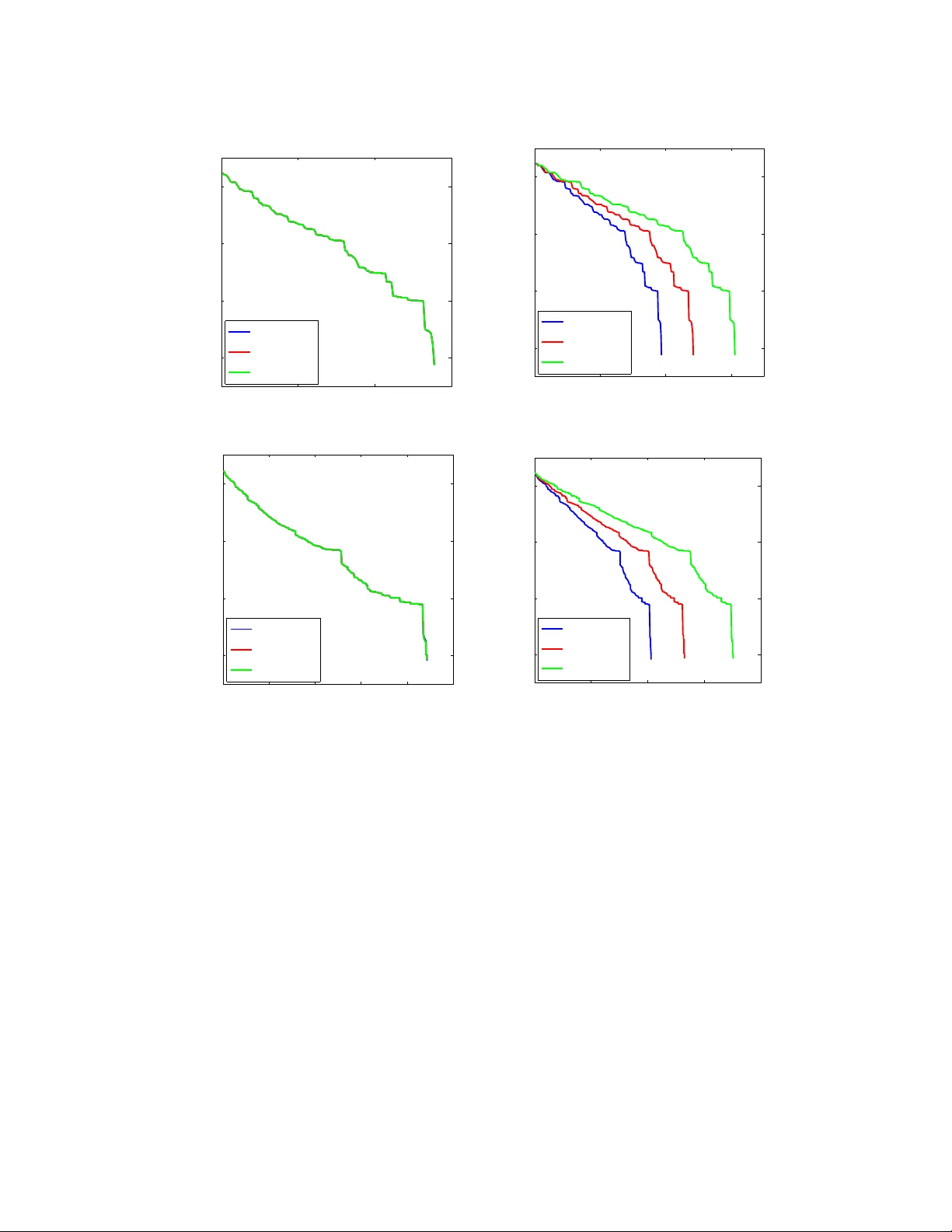
Inexact Co ordinate Descen t: Complexit y and Preconditioning ∗ Rac hael T app enden P eter Ric ht´ arik Jacek Gondzio Scho ol of Mathematics University of Edinbur gh Unite d Kingdom Decem b er 11, 2014 Abstract In this pap er w e consider the problem of minimizing a conv ex function using a randomized blo c k co ordinate descent metho d. One of the key steps at each iteration of the algorithm is determining the up date to a blo c k of v ariables. Existing algorithms assume that in order to compute the up date, a particular subproblem is solved exactly . In this work we relax this re- quiremen t, and allo w for the subproblem to b e solved inexactly , leading to an inexact blo c k co ordinate descent metho d. Our approach incorp orates the b est known results for exact up- dates as a sp ecial case. Moreo ver, these theoretical guarantees are complemented by practical considerations: the use of iterative techniques to determine the update as w ell as the use of preconditioning for further acceleration. Keyw ords: inexact methods, block coordinate descent, conv ex optimization, iteration com- plexit y , preconditioning, conjugate gradients. AMS: 65F08; 65F10; 65F15; 65Y20; 68Q25; 90C25 1 In tro duction Due to a dramatic increase in the size of optimization problems b eing encoun tered, ﬁrst order metho ds are becoming increasingly p opular. These large-scale problems are often highly structured and it is imp ortan t for any optimization metho d to take adv an tage of the underlying structure. Applications where such problems arise and where ﬁrst order metho ds ha ve pro ved successful include mac hine learning [17, 33], compressiv e sensing [8, 43], group lasso [26, 36], matrix completion [5, 27], and truss top ology design [28]. Blo c k co ordinate descen t metho ds seem a natural c hoice for these very large-scale problems due to their low memory requirements and lo w p er-iteration computational cost. F urthermore, they are often designed to tak e adv an tage of the underlying structure of the optimization problem [41, 42] and man y of these algorithms are supp orted by high probabilit y iteration complexit y results [24, 25, 28, 29, 38]. ∗ This work was supp orted b y the EPSRC grant EP/I017127/1 “Mathematics for v ast digital resources”. P eter Ric ht´ arik was also supp orted by the Centre for Numerical Algorithms and Intelligen t Softw are (funded by EPSR C gran t EP/G036136/1 and the Scottish F unding Council). 1 1.1 The Problem If the blo ck size is larger than one, determining the up date to use at a particular iteration in a blo c k co ordinate descen t metho d can be computationally exp ensiv e. The purp ose of this work is to reduce the cost of this step. T o achiev e this, w e extend the work in [29] to include the case of an inexact up date. In this work w e study randomized blo c k co ordinate descen t methods applied to the problem of minimizing a comp osite ob jective function. That is, a function formed as the sum of a smo oth con vex and a simple nonsmo oth conv ex term: min x ∈ R N { F ( x ) := f ( x ) + Ψ( x ) } . (1) W e assume that the problem has a minim um ( F ∗ > −∞ ), f has (blo c k) coordinate Lipschitz gradien t, and Ψ is a (block) separable prop er closed conv ex extended real v alued function (all these concepts will b e deﬁned precisely in Section 2). Our algorithm (namely , the Inexact Co ordinate Descen t (ICD) metho d) is supp orted by high probabilit y iteration complexit y results. That is, for conﬁdence level ρ ∈ (0 , 1) and error tolerance  > 0, w e give an explicit expression for the num ber of iterations k that guarantee that the ICD metho d pro duces a random iterate x k for which P ( F ( x k ) − F ∗ ≤  ) ≥ 1 − ρ. W e will show that in the inexact case it is not alwa ys p ossible to achiev e a solution with small error and/or high conﬁdence. Our theoretical guarantees are complemented by practical considerations. In Section 3.3 we explain our inexactness condition in detail and in Section 3.4 we giv e examples to show when the inexactness condition is implemen table. F urther, in Section 6 we give sev eral examples, deriv e the up date subproblems, and suggest algorithms that could be used to solv e the subproblems inexactly . Finally , w e presen t some encouraging computational results. 1.2 Literature Review As problem sizes increase, ﬁrst order metho ds are b eneﬁting from revived interest. On very large problems ho wev er, the computation of a single gradient step is exp ensiv e, and metho ds are needed that are able to mak e progress b efore a standard gradien t algorithm tak es a single step. F or instance, a randomized v arian t of the Kaczmarz metho d for solving linear systems has recen tly b een studied, equipp ed with iteration complexit y b ounds [21, 22, 16, 37], and found to b e surprisingly eﬃcient. This metho d can b e seen as a special case of a more general class of decomp osition algorithms, blo c k co ordinate descent methods, which hav e recen tly gained m uch p opularity [20, 24, 25, 29, 30, 31, 40]. One of the main diﬀerences b et ween v arious (serial) co ordinate descen t sc hemes is the wa y in which the co ordinate is c hosen at eac h iteration. T raditionally cyclic schemes [32] and greedy sc hemes [28] were studied. More recently , a p opular alternative is to select co ordinates randomly , b ecause the co ordinate can b e selected cheaply , and useful iteration complexit y results can be obtained [19, 29, 30, 31, 39, 35]. Another current trend in this area is to consider methods that incorporate some kind of ‘inexact- ness’, p erhaps using appro ximate gradients, or using inexact up dates. F or example, [18] considers metho ds based on inexact dual gradient information, while [33] considers the minimization of an 2 unconstrained con vex composite function where error is presen t in the gradien t of the smo oth term, or in the pro ximity op erator for the non-smo oth term. Other works study metho ds that use in- exact up dates when the ob jective function is con vex, smo oth and unconstrained [1], smo oth and constrained [3] or for ` 1 -regularized quadratic least squares problem [15]. 1.3 Con tribution In this pap er we extend the work of Ric ht´ arik and T ak´ a ˇ c [29] and presen t a block co ordinate descent metho d that emplo ys inexact up dates ha ving the p otential to reduce the o verall algorithm running time. F urthermore, w e fo cus in detail on the quadratic case, which b eneﬁts greatly from inexact up dates, and show how preconditioning can b e used to complemen t the inexact up date strategy . F Exact Metho d [29] Inexact Metho d [this pap er] Theorem C-N c 1   1 + log 1 ρ  + 2 c 1  − u + c 1  − αc 1 log  − β c 1  − αc 1 ρ − β c 1  − αc 1 ! + 2 9(i) C-N c 2 log  F ( x 0 ) − F ∗ ρ  c 2 1 − αc 2 log F ( x 0 ) − F ∗ − β c 2 1 − αc 2 ρ − β c 2 1 − αc 2 ! 9(ii) SC-N n µ log  F ( x 0 ) − F ∗ ρ  n µ − αn log F ( x 0 ) − F ∗ − β n µ − αn ρ − β n µ − αn ! 11 C-S ˆ c 1   1 + log 1 ρ  + 2 ˆ c 1  − ˆ u + ˆ c 1  − α ˆ c 1 log  − β ˆ c 1  − α ˆ c 1 ρ − β ˆ c 1  − α ˆ c 1 ! + 2 12 SC-S 1 µ f log  f ( x 0 ) − f ∗ ρ  1 µ f − α log   f ( x 0 ) − f ∗ − β µ f − α ρ − β µ f − α   13 T able 1: Comparison of the iteration complexity results for co ordinate descent metho ds using an inexact up date and using an exact up date (C=Con vex, SC=Strongly Con vex, N=Nonsmo oth, S = Smo oth). T able 1 compares some of the new complexit y results obtained in this pap er for an inexact up date with the complexit y results for an exact up date presented in [29]. The follo wing notation is used in the table: b y µ φ w e denote the strong conv exity parameter of function φ (with resp ect to a certain norm sp eciﬁed later), µ = ( µ f + µ Ψ ) / (1 + µ Ψ ) and R w ( x 0 ) can b e roughly considered to b e distance from x 0 to a solution of (1) measured in a sp eciﬁc w eighted norm parameterized by the v ector w (to be deﬁned precisely in (14)). The constants are c 1 = 2 n max {R 2 w ( x 0 ) , F ( x 0 ) − F ∗ } , ˆ c 1 = 2 R 2 w ( x 0 ) and c 2 = 2 n R 2 w ( x 0 ) / , and n is the n umber of blo c ks. Parameters α, β ≥ 0 control the lev el of inexactness (to b e deﬁned precisely in Section 3.2) and u and ˆ u are constants dep ending on α , β and c 1 , and α , β and ˆ c 1 , resp ectiv ely . T able 1 shows that for ﬁxed  and ρ , an inexact metho d will require more iterations than an exact one. Ho wev er, it is exp ected that in certain situations an inexact update will b e signiﬁcantly c heap er to compute than an exact up date, leading to b etter o verall running time. Moreov er, the new complexity results for the inexact metho d generalize those for the exact metho d. Sp eciﬁcally , 3 for inexactness parameters α = β = 0 we reco ver the complexity results in [29]. 1.4 Outline The ﬁrst part of this pap er fo cuses on the theoretical asp ects of a blo c k co ordinate descent metho d when an inexact up date is emplo yed. In Section 2 the assumptions and notation are laid out and in Section 3 the ICD metho d is presented. In Section 4 iteration complexity results for ICD applied to (1) are presented in b oth the con vex and strongly con vex cases. Iteration complexity results for ICD applied to a conv ex smo oth minimization problem (Ψ = 0 in (1)) are presen ted in Section 5, in b oth the conv ex and strongly con vex cases. The second part of the pap er considers the practicalit y of an inexact up date. Section 6 pro vides sev eral examples of ho w to derive the form ulation for the up date step subproblem, as well as giving suggestions for algorithms that can b e used to solve the subproblem inexactly . Numerical exp erimen ts are presen ted in Section 7 and Appendix A pro vides a detailed analysis of the sp ectrum of the preconditioned matrix used in the numerical exp erimen ts. 2 Assumptions and Notation In this section w e introduce the notation and deﬁnitions that are used throughout the pap er. 2.1 Blo c k structure of R N The problem under consideration is assumed to ha ve blo c k structure and this is mo delled b y decomp osing the space R N in to n subspaces as follo ws. Let U ∈ R N × N b e a column p ermutation of the N × N iden tity matrix and further let U = [ U 1 , U 2 , . . . , U n ] b e a decomp osition of U into n submatrices, where U i is N × N i and P n i =1 N i = N . It is clear (e.g., see [30] for a brief pro of ) that an y vector x ∈ R N can b e written uniquely as x = n X i =1 U i x ( i ) , (2) where x ( i ) ∈ R N i . Moreov er, these v ectors are giv en by x ( i ) := U T i x. (3) F or simplicity w e will sometimes write x = ( x (1) , x (2) , . . . , x ( n ) ) instead of (2). W e equip R N i with a pair of conjugate norms, induced b y a quadratic form inv olving a symmetric positive deﬁnite matrix B i : k t k ( i ) := h B i t, t i 1 2 , k t k ∗ ( i ) = h B − 1 i t, t i 1 2 , t ∈ R N i , (4) where h· , ·i is the standard Euclidean dot pro duct. 2.2 Smo othness of f Throughout this pap er we assume that the gradient of f is blo c k Lipschitz, uniformly in x , with p ositiv e constants l 1 , . . . , l n . This means that, for all x ∈ R N , i ∈ { 1 , 2 , . . . , n } and t ∈ R N i w e ha ve k∇ i f ( x + U i t ) − ∇ i f ( x ) k ∗ ( i ) ≤ l i k t k ( i ) , (5) 4 where ∇ i f ( x ) := ( ∇ f ( x )) ( i ) (3) = U T i ∇ f ( x ) ∈ R N i . (6) An imp ortan t consequence of (5) is the following standard inequalit y [23, p.57]: f ( x + U i t ) ≤ f ( x ) + h∇ i f ( x ) , t i + l i 2 k t k 2 ( i ) . (7) 2.3 Blo c k separability of Ψ The function Ψ : R N → R ∪ { + ∞} is assumed to b e blo c k separable. That is, we assume that it can b e decom posed as: Ψ( x ) = n X i =1 Ψ i ( x ( i ) ) , (8) where the functions Ψ i : R N i → R ∪ { + ∞} are con vex and closed. 2.4 Norms on R N F or ﬁxed p ositive scalars w 1 , w 2 , . . . , w n , let w = ( w 1 , . . . , w n ) and deﬁne a pair of conjugate norms in R N b y k x k 2 w := n X i =1 w i k x ( i ) k 2 ( i ) , ( k y k ∗ w ) 2 := max k x k w ≤ 1 h y , x i 2 = n X i =1 w − 1 i ( k y ( i ) k ∗ ( i ) ) 2 . (9) In the subsequen t analysis we will often use w = l (for Ψ 6 = 0) and/or w = l p − 1 (for Ψ = 0), where l = ( l 1 , . . . , l n ) is a v ector of Lipschitz constants, p = ( p 1 , . . . , p n ) is a v ector of p ositiv e probabilities and l p − 1 denotes the vector ( l 1 /p 1 , . . . , l n /p n ). 2.5 Strong conv exit y of F A function φ : R N → R ∪ { + ∞} is strongly conv ex w.r.t. k · k w with conv exity parameter µ φ ( w ) > 0 if for all x, y ∈ dom φ , φ ( y ) ≥ φ ( x ) + h φ 0 ( x ) , y − x i + µ φ ( w ) 2 k y − x k 2 w , (10) where φ 0 is any subgradient of φ at x . The case with µ φ ( w ) = 0 reduces to conv exit y . In some of the results presented in this w ork we assume that F is strongly con vex. Strong con vexit y of F ma y come from f or Ψ or b oth and we will write µ f ( w ) (resp. µ Ψ ( w )) for the strong con vexit y parameter of f (resp. Ψ), with resp ect to k · k w . F ollowing from (10) µ F ( w ) ≥ µ f ( w ) + µ Ψ ( w ) . (11) Using (7) and (10) it can b e shown that µ f ( l ) ≤ 1 , and µ f ( lp − 1 ) < 1 . (12) W e will also mak e use of the follo wing characterisation of strong con vexit y . F or all x, y ∈ dom φ and λ ∈ [0 , 1], φ  λx + (1 − λ ) y  ≤ λφ ( x ) + (1 − λ ) φ ( y ) − µ φ ( w ) λ (1 − λ ) 2 k x − y k 2 w . (13) 5 2.6 Lev el set radius The set of optimal solutions of (1) is denoted by X ∗ and x ∗ is any element of that set. W e deﬁne R w ( x ) := max y max x ∗ ∈ X ∗ {k y − x ∗ k w : F ( y ) ≤ F ( x ) } , (14) whic h is a measure of the size of the level set of F giv en by x . W e assume that R w ( x 0 ) is ﬁnite for the initial iterate x 0 . 3 The Algorithm Let us start b y presenting the algorithm; a more detailed description will follow. Algorithm 1 ICD: Inexact Co ordinate Descent 1: Input: Inexactness parameters α, β ≥ 0, and probabilities p 1 , . . . , p n > 0. 2: for k = 0 , 1 , 2 , . . . do 3: Cho ose δ k = ( δ (1) k , . . . , δ ( n ) k ) ∈ R n according to (20) 4: Cho ose blo c k i ∈ { 1 , 2 , . . . , n } with probabilit y p i 5: Compute the inexact up date T ( i ) δ k ( x k ) to blo c k i of x k 6: Up date blo c k i of x k : x k +1 = x k + U i T ( i ) δ k ( x k ) 7: end for 3.1 Generic description Giv en iterate x k ∈ R N , Algorithm 1 picks blo ck i ∈ { 1 , 2 , . . . , n } with probability p i , computes the up date v ector T ( i ) δ k ( x k ) ∈ R N i (w e commen t on ho w this is computed later in this section) and then adds it to the i th blo c k of x k , pro ducing the new iterate x k +1 . The iterates { x k } are random vectors and the v alues { F ( x k ) } are random v ariables. The up date v ector dep ends on x k , the curren t iterate, and on δ k , a v ector of parameters con trolling the “lev el of inexactness” with whic h the up date is computed. The rest of this section is devoted to giving a precise deﬁnition of T ( i ) δ k ( x k ). Note that from (1) and (7) we ha ve, for all x ∈ R N , i ∈ { 1 , 2 , . . . , n } and t ∈ R N i : F ( x + U i t ) = f ( x + U i t ) + Ψ( x + U i t ) ≤ f ( x ) + V i ( x, t ) + Ψ − i ( x ) , (15) where V i ( x, t ) := h∇ i f ( x ) , t i + l i 2 k t k 2 ( i ) + Ψ i ( x ( i ) + t ) , (16) Ψ − i ( x ) := X j 6 = i Ψ j ( x ( j ) ) . (17) That is, (15) giv es an upp er b ound on F ( x + U i t ), viewed as a function of t ∈ R N i . The inexact up date computed in Step 5 of Algorithm 1 is the inexact minimizer of the upp er b ound (15) on F ( x k + U i t ) (to b e deﬁned precisely b elo w). Ho wev er, since only the second term of this b ound dep ends on t , the up date is computed by minimizing, inexactly , V i ( x, t ) in t . 6 3.2 Inexact up date The approach of this pap er b est applies to situations in which it is m uch easier to approximately minimize t 7→ V i ( x, t ) than to either (i) appro ximately minimize t 7→ F ( x + U i t ) and/or (ii) exactly minimize t 7→ V i ( x, t ). F or x ∈ R N and δ = ( δ (1) , . . . , δ ( n ) ) ≥ 0 we deﬁne T δ ( x ) := ( T (1) δ ( x ) , . . . , T ( n ) δ ( x )) ∈ R N to b e any vector satisfying V i ( x, T ( i ) δ ( x )) ≤ min  V i ( x, 0) , δ ( i ) + min t ∈ R N i V i ( x, t )  , i = 1 , . . . , n. (18) (W e allo w here for an abuse of notation — δ ( i ) is a scalar, rather than a vector in R N i as x ( i ) for x ∈ R N — b ecause w e wish to emphasize that the scalar δ ( i ) is asso ciated with the i th block.) That is, we require that the inexact up date T ( i ) δ ( x ) of the i th blo c k of x is (i) no w orse than a v acuous up date, and that it is (ii) close to the optimal up date T ( i ) 0 ( x ) = arg min t V i ( x, t ), where the degree of sub optimalit y/inexactness is b ounded by δ ( i ) . As the following lemma shows, the up date (18) leads to a monotonic algorithm. Lemma 1. F or al l x ∈ R N , δ ∈ R n + and i ∈ { 1 , 2 , . . . , n } , F ( x + U i T ( i ) δ ( x )) ≤ F ( x ) . (19) Pr o of: F ( x + U i T ( i ) δ ( x )) (15) ≤ f ( x ) + V i ( x, T ( i ) δ ( x )) + Ψ − i ( x ) (18) ≤ f ( x ) + V i ( x, 0) + Ψ − i ( x ) (16)+(17) = F ( x ) . F urthermore, in this w ork we provide iteration complexity results for ICD, where δ k = ( δ (1) k , . . . , δ ( n ) k ) is chosen in such a w ay that the exp ected sub optimality is b ounded ab o v e b y a linear function of the residual F ( x k ) − F ∗ . That is, we hav e the following assumption. Assumption 2. F or constants α, β ≥ 0, the vector δ k = ( δ (1) k , . . . , δ ( n ) k ) is chosen to satisfy ¯ δ k := n X i =1 p i δ ( i ) k ≤ α ( F ( x k ) − F ∗ ) + β , (20) Notice that, for instance, Assumption 2 holds if w e require δ ( i ) k ≤ α ( F ( x k ) − F ∗ ) + β for all blo c ks i and iterations k . The motiv ation for allowing inexact up dates of the form (18) is that calculating exact up dates is imp ossible in some cases (for example, not all problems hav e a closed form solution), and com- putationally in tractable in others. The purp ose of allowing inexactness in the up date step of ICD is that an iter ative metho d can b e used to solv e for the up date T ( i ) δ ( x ), thus signiﬁcantly expanding the range of problems that can b e successfully tackled by co ordinate descent. In this case, there is an outer co ordinate descent loop, and an inner iterative lo op to determine the up date. Assumption 2 shows that the stopping tolerance on the inner lo op, must b e b ounded ab o ve via (20). CD methods pro vide a mechanism to break up v ery large/h uge scale problem, into smaller pieces that are a fraction of the total dimension. Moreo ver, often the subproblems that arise to 7 solv e for the update ha ve a similar/the same form as the original huge scale problem. (F or example, see the numerical exp eriments in Section 7, and the examples given in Section 6.) There are many iterativ e metho ds that cannot scale up to the original huge dimensional problem, but are excellen t at solving the medium scale up date subproblems. ICD allows these algorithms to solve for the up date at eac h iteration, and if the up dates are solv ed eﬃcien tly , then the ov erall ICD algorithm running time is k ept low. 3.3 The role of α and β in ICD The condition (18) shows that the up dates in ICD are inexact , while Assumption 2 giv es the level of inexactness that is allow ed in the computed update. Moreo ver, Assumption 2 allo ws us to provide a uniﬁed analysis; formulating the error/inexactness expression in this general w ay (20) gives insight in to the role of b oth multiplic ative and additive err or , and how this err or pr op agates through the algorithm as iterates progress. F ormulation (20) is in teresting from a theoretical p erspective b ecause it allo ws us to presen t a sensitivity analysis for ICD, which is interesting in its own righ t. Ho wev er, we stress that (18), coupled with Assumption 2, is muc h more than just a tec hnical to ol; α and β are actually parameters of the ICD algorithm (Algorithm 1) that can b e assigned explicit numeric al values in many cases. W e no w explain (18), Assumption 2 and the role of parameters α and β in slightly more detail. (Note that α and β m ust b e c hosen suﬃcien tly small to guarantee con verge of the ICD algorithm. Ho wev er, we p ostp one discussion of the magnitude of α and β un til Section 3.5.) There are four cases. 1. Case I: α = β = 0 . This corresp onds to the exact c ase where no err or is allow ed in the computed up date. 2. Case I I: α = 0 , β > 0 . This case corresp onds to additiv e error only , where the error lev el β > 0 is ﬁxed at the start of Algorithm 1. In this case, (18) and (20) sho w that the error allo wed in the inexact up date T ( i ) δ ( x k ) is on aver age β . F or example, one can set δ ( i ) k = β , for all blo c ks i and all iterations k so that (20) b ecomes ¯ δ k = P i p i β = β . Notice that the tolerance allow able on each blo c k need not b e the same; if one sets δ ( i ) k ≤ β , for all blo c ks i and iterates k then ¯ δ k ≤ β , so (20) holds true. Moreo ver, one need not set δ ( i ) k > 0 for all i , so that the update v ector T ( i ) δ ( x k ) could b e exact for some blo c ks ( δ ( i ) k = 0), and inexact for others ( δ ( j ) k > 0). (This ma y b e sensible, for example, when Ψ i ( x ( i ) ) 6 = Ψ j ( x ( j ) ) for some i 6 = j and that (16) has a closed form solution for T ( i ) ( x k ) but not for T ( j ) ( x k ).) F urthermore, consider the extreme case where only one blo c k up date is inexact T ( i ) δ ( x k ), ( T ( j ) 0 ( x k ) for all j 6 = i ). If the co ordinates are selected with uniform probabilit y , then the inexactness lev el on blo c k i can b e as large as δ ( i ) k = nβ and Assumption 2 holds. 3. Case I I I: α > 0 , β = 0 . In this case only m ultiplicative error is allow ed in the computed up date T ( i ) δ ( x k ), where the error allo wed in the up date at iteration k is related to the error in the function v alue ( F ( x k ) − F ∗ ). The multiplicativ e error level α is ﬁxed at the start of Algorithm 1, and α ( F ( x k ) − F ∗ ) is an upper bound on the a verage error in the update T ( i ) δ ( x k ) o ver all blo cks i at iteration k . In particular, notice that setting δ ( i ) k ≤ α ( F ( x k ) − F ∗ ), for all i and k satisﬁes Assumption 2. As for Case I I, one is allow ed to set δ ( i ) k = 0 for some block(s) 8 i , or to set δ ( i ) k > α ( F ( x k ) − F ∗ ) for some blo c ks i and iterations k as long as Assumption 2 is satisﬁed. 4. Case IV: α > 0 , β > 0 . This is the most general case, corresp onding to the inclusion of b oth m ultiplicative and additiv e error, where the error level parameters α and β are ﬁxed at the start of Algorithm 1. Notice that Assumption 2 is satisﬁed when the error δ ( i ) k in the computed up date T ( i ) δ ( x k ) ob eys δ ( i ) k ≤ α ( F ( x k ) − F ∗ ) + β . Moreov er, as for Cases I I and I II, one is allow ed to set δ ( i ) k = 0 for some blo ck(s) i , or to set δ ( i ) k > α ( F ( x k ) − F ∗ ) for some blo c ks i and iterations k as long as Assumption 2 is satisﬁed. Notice that, as iterations progress, the multiplicativ e error α may b ecome dominated by the additive error β , in the sense that, α ( F ( x k ) − F ∗ ) → 0 as k → ∞ so the upp er b ound on ¯ δ k tends to β . Cases I–IV ab ov e show that the parameters α and β directly relate to the stopping criterion used in the algorithm employ ed to solv e for the up date T ( i ) δ ( x k ) at eac h iteration of ICD. The follo wing section gives examples of algorithms that can b e used within ICD, where α and β can b e giv en explicit n umerical v alues and the stopping tolerances are veriﬁable. 3.4 Computing the inexact up date In this section w e fo cus on the computation of the inexact up date (Step 5 of Algorithm 1). W e discuss several cases where it is p ossible to verify Assumption 2, and th us provide speciﬁc instances to show that ICD is indeed implemen table. In order to compute an inexact up date, the quan tity V i ( x, T ( i ) 0 ( x k )) in (18) is needed. Moreo ver, to incorp orate multiplicativ e error, the optimal ob jective v alue F ∗ m ust also b e kno wn. 1. F ∗ is known: There are many instances when F ∗ is known a priori, which means that the b ound F ( x k ) − F ∗ is computable at every iteration, and subsequently multiplicativ e error can b e incorporated in to ICD. In most cases, the update subproblem (18) has the same form as the original problem (see Section 6), so that V i ( x k , T ( i ) 0 ) is also kno wn. This is the case, for example, when solving a consistent system of equations (minimizing a quadratic function), where F ∗ = 0, so that F ( x k ) − F ∗ = F ( x k ). The up date subproblem has the same form (a consistent system of equations m ust b e solv ed to calculate T ( i ) δ k ), so we also ha ve V i ( x k , T ( i ) 0 ) = 0. Hence, for an y α, β ≥ 0, one can compute δ ( i ) k (20), that satisﬁes Assumption 2 and (18). That is, at each iteration of ICD, accept any inexact up date T ( i ) δ k that satisﬁes: V i ( x k , T ( i ) δ k ) − V i ( x k , T ( i ) 0 ) = V i ( x k , T ( i ) δ k ) ≤ δ ( i ) k ≤ αF ( x k ) + β . (21) 2. Primal-dual algorithm: If the up date T ( i ) δ k is found using an algorithm that terminates on the duality gap, then (18) and Assumption 2 are easy to verify . In particular, supp ose that α = 0 and β > 0 is ﬁxed when initializing ICD. Then, for blo c k i and iteration k , we accept T ( i ) δ k suc h that V i ( x k , T ( i ) δ k )) − V i ( x k , T ( i ) 0 ) ≤ V i ( x k , T ( i ) δ k )) − V DUAL i ( x k , T ( i ) δ k )) ≤ δ ( i ) k ≤ β , (22) where V DUAL i ( x k , T ( i ) δ k )) is the v alue of the dual at the p oin t T ( i ) δ k . 9 Remark 3. 1. Both (21) and (22) are termination criteria for the iterative metho d used for the inner lo op to determine the inexact up date T ( i ) δ ( x k ). They show that the error b ound is indeed implementable , and that the inexactness parameters α and β relate to the stopping tolerance used in the inner lo op of ICD. 2. Selecting an appropriate stopping criterion and tolerance (i.e., deciding upon n umerical v alues for α and β ) is a problem that frequently arises when solving optimization problems, and the decision is left to the discretion of the user. 3. It ma y b e p ossible to ﬁnd other stopping conditions such that (18) is veriﬁable. Moreov er, it ma y b e p ossible for the algorithm to conv erge in pr actic e if a stopping condition is used for whic h (18) cannot b e chec ked. 3.5 T ec hnical result The following result pla ys a k ey role in the complexit y analysis of ICD. Theorem 4. Fix x 0 ∈ R N and let { x k } k ≥ 0 b e a se quenc e of r andom ve ctors in R N with x k +1 dep ending on x k only. L et ϕ : R N → R b e a nonne gative function, deﬁne ξ k := ϕ ( x k ) and assume that { ξ k } k ≥ 0 is nonincr e asing. F urther, let ρ ∈ (0 , 1) ,  > 0 and α , β ≥ 0 b e such that one of the fol lowing two c onditions holds: (i) E [ ξ k +1 | x k ] ≤ (1 + α ) ξ k − ξ 2 k c 1 + β , for al l k ≥ 0 , wher e c 1 > 0 , c 1 2  α + q α 2 + 4 β c 1 ρ  <  < min { (1 + α ) c 1 , ξ 0 } and σ := q α 2 + 4 β c 1 < 1 ; (ii) E [ ξ k +1 | x k ] ≤  1 + α − 1 c 2  ξ k + β , for al l k ≥ 0 for which ξ k ≥  , wher e αc 2 < 1 ≤ (1 + α ) c 2 , and β c 2 ρ (1 − αc 2 ) <  < ξ 0 . If ( i ) holds and we deﬁne u := c 1 2 ( α + σ ) and cho ose K ≥ c 1  − αc 1 log  − β c 1  − αc 1 ρ − β c 1  − αc 1 ! + min  1 σ log  ξ 0 − u  − u  , c 1  − u − c 1 ξ 0 − u  + 2 , (23) (wher e the se c ond term in the minimum is chosen if σ = 0 ), or if ( ii ) holds and we cho ose K ≥ c 2 1 − αc 2 log ξ 0 − β c 2 1 − αc 2 ρ − β c 2 1 − αc 2 ! , (24) then P ( ξ K ≤  ) ≥ 1 − ρ . Pr o of. First notice that the thresholded sequence { ξ  k } k ≥ 0 deﬁned by ξ  k = ( 0 , if ξ k < , ξ k , otherwise, (25) satisﬁes ξ  k >  ⇔ ξ k >  . Therefore, by Mark ov’s inequalit y , P ( ξ k >  ) = P ( ξ  k >  ) ≤ E [ ξ  k ]  . Letting θ k := E [ ξ  k ], it thus suﬃces to show that θ K ≤ ρ. (26) 10 (The rationale b ehind this “thresholding trick” is that the sequence E [ ξ  k ] decreases faster than E [ ξ k ] and hence will reach ρ so oner.) Assume now that (i) holds. It can b e shown (for example, see Theorem 1 of [29] for the case α = β = 0) that E [ ξ  k +1 | x k ] ≤ (1 + α ) ξ  k − ( ξ  k ) 2 c 1 + β , E [ ξ  k +1 | x k ] ≤  1 + α −  c 1  ξ  k + β . (27) By taking exp ectations in (27) (in x k ) and using Jensen’s inequality , we obtain θ k +1 ≤ (1 + α ) θ k − θ 2 k c 1 + β , k ≥ 0 , (28) θ k +1 ≤  1 + α −  c 1  θ k + β , k ≥ 0 . (29) Notice that (28) is b etter than (29) precisely when θ k >  . It is easy to see that the inequality (1 + α ) θ k − θ 2 k c 1 + β ≤ θ k holds if and only if θ k ≥ u . In other w ords, (28) leads to θ k +1 that is b etter than θ k only for θ k ≥ u . W e will no w compute k = k 1 for whic h u < θ k ≤  . Inequalit y (28) can b e equiv alently written as θ k +1 − u ≤ (1 − σ )( θ k − u ) − ( θ k − u ) 2 c 1 , k ≥ 0 . (30) where σ < 1. W riting (28) in the form (30) eliminates the constan t term β , whic h allows us to pro vide a simple analysis. (Moreov er, this “shifted” form leads to a b etter result; see the remarks after the Theorem for details.) Letting ˆ θ k := θ k − u , b y monotonicit y w e ha ve ˆ θ k +1 ˆ θ k ≤ ˆ θ 2 k , whence 1 − σ ˆ θ k +1 − 1 ˆ θ k = (1 − σ ) ˆ θ k − ˆ θ k +1 ˆ θ k +1 ˆ θ k ≥ (1 − σ ) ˆ θ k − ˆ θ k +1 ˆ θ 2 k (30) ≥ 1 c 1 . (31) If we choose r ∈ { 1 , 1 1 − σ } , then 1 ˆ θ k (31) ≥ r 1 ˆ θ k − 1 + 1 c 1 ! ≥ r k 1 ˆ θ 0 + 1 c 1 k X j =1 r j = ( r k  1 ξ 0 − u + 1 c 1 σ  − 1 c 1 σ , r = 1 1 − σ , 1 ξ 0 − u + k c 1 , r = 1 . In particular, using the ab ov e estimate with r = 1 and r = 1 1 − σ giv es ˆ θ k 1 ≤  − u (and hence θ k 1 ≤  ) (32) for k 1 := min (& log 1  − u + 1 c 1 σ 1 ξ 0 − u + 1 c 1 σ ! / log  1 1 − σ  ' ,  c 1  − u − c 1 ξ 0 − u  ) , (33) where the left term in (33) applies when σ > 0 only . Applying the inequalities (i) d t e ≤ 1 + t ; (ii) log ( 1 1 − t ) ≥ t (holds for 0 < t < 1; w e use the in verse v ersion, whic h is surprisingly tigh t for small t ); and (iii) the fact that t 7→ C + t D + t is decreasing on [0 , ∞ ) if C ≥ D > 0, we arriv e at the following b ound k 1 ≥ 1 + min  1 σ log  ξ 0 − u  − u  , c 1  − u − c 1 ξ 0 − u  . (34) 11 Letting γ := 1 −  − αc 1 c 1 (notice that γ ∈ (0 , 1)), for any k 2 ≥ 0 we ha ve θ k 1 + k 2 (29) ≤ γ θ k 1 + k 2 − 1 + β ≤ γ k 2 θ k 1 + β ( γ k 2 − 1 + γ k 2 − 2 + · · · + 1) (32) ≤ γ k 2  + β 1 − γ k 2 1 − γ = γ k 2   − β 1 − γ  + β 1 − γ . (35) In (35), notice that the second to last term can b e made as small as we lik e (by taking k 2 large), but w e can never force θ k 1 + k 2 ≤ β 1 − γ . Therefore, in order to establish (26), we need to ensure that β c 1  − αc 1 < ρ . Rearranging this gives the condition c 1 2 ( α + q α 2 + 4 β c 1 ρ ) <  , which holds b y assumption. Now w e can ﬁnd k 2 for which the righ t hand side in (35) is at most ρ : k 2 := & log  − β 1 − γ ρ − β 1 − γ ! / log  1 γ  ' ≤ 1 + c 1  − αc 1 log  − β c 1  − αc 1 ρ − β c 1  − αc 1 ! . (36) In view of (26), it is enough to take K = k 1 + k 2 iterations. The expression in (23) is obtained b y adding the upp er b ounds on k 1 and k 2 in (34) and (36). No w assume that prop ert y ( ii ) holds. By a similar argumen t as that leading to (27), w e obtain θ K ≤  1 − 1 − αc 2 c 2  θ K − 1 + β ≤  1 − 1 − αc 2 c 2  K θ 0 + β K − 1 X j =0  1 − 1 − αc 2 c 2  j ≤  1 − 1 − αc 2 c 2  K  θ 0 − β c 2 1 − αc 2  + β c 2 1 − αc 2 (24) ≤ ρ. The pro of follows by taking K giv en b y (24). Let us now commen t on sev eral asp ects of the ab o ve result: 1. Usage. W e will use Theorem 4 to ﬁnish the pro ofs of the complexity results in Section 4; with ξ k = ϕ ( x k ) := F ( x k ) − F ∗ , where { x k } is the random pro cess generated by ICD. 2. Monotonicity and Nonne gativity. Note that the monotonicity assumption in Theorem 4 is for the c hoice of x k and ϕ described in 1) satisﬁed due to (19). Nonnegativity is satisﬁed automatically since F ( x k ) ≥ F ∗ for all x k . 3. Best of two. In (33), w e notice that the ﬁrst term applies when σ > 0 only . If σ = 0, then u = 0, and subsequently the second term in (33) applies, which corresponds to the exact case. Notice that if σ > 0 is v ery small (so u 6 = 0), the iteration complexit y result still ma y b e b etter if the second term is used. 4. Gener alization. Note that for α = β = 0, (23) reco vers c 1  (1 + log 1 ρ ) + 2 − c 1 ξ 0 , which is the result prov ed in Theorem 1(i) in [29], while (24) reco vers c 2 log(( F ( x 0 ) − F ∗ ) /ρ ), whic h is the result prov ed in Theorem 1(ii) in [29]. Since the last term in (23) is negativ e, the theorem holds also if w e ignore it. This is what we ha ve done, for simplicity , in T able 1. 5. High ac cur acy with high pr ob ability. In the exact case, the iteration complexity results hold for any error tolerance  > 0 and conﬁdence ρ ∈ (0 , 1). Ho wev er, in the inexact case, there 12 are restrictions on the c hoice of ρ and  for which w e can guarantee the result P ( F ( x k ) − F ∗ ≤  ) ≥ 1 − ρ . T able 5 gives conditions on α and β under which arbitrary conﬁdence lev el (i.e., small ρ ) and accuracy (i.e., small  ) is achiev able. F or instance, if Theorem 4(ii) is used, then one can achiev e arbitrary accuracy only if β = 0, but arbitrary conﬁdence under no assumptions on α and β . The situation for part (i) is worse:  is lo wer b ounded by a p ositiv e expression that inv olves ρ , unless α = β = 0. Theorem 4(i) Theorem 4(ii)  can b e arbitrarily small if α = β = 0 β = 0 ρ can b e arbitrarily small if β = 0 an y α, β T able 2: The conditions under which arbitrary conﬁdence ρ and accuracy  are attainable. 6. Two lower b ounds on  . The inequality  > c 1 2  α + q α 2 + 4 β ρc 1  (see part (i) of Theorem 4) is equiv alen t to  > β c 1 ρ (  − αc 1 ) . Note the similarit y of the last expression and the low er b ound on  in part (ii) of the theorem. W e can see that the low er b ound on  is smaller (and hence, is less restrictive) in (ii) than in (i), provided that c 1 = c 2 . 7. Two analyses. It can b e seen that analyzing the “shifted” form (30) leads to a b etter result than analyzing (28) directly , ev en when β = 0. Consider the case β = 0, so that σ = α and u = αc 1 . F rom equation (31) θ k +1 ≤ A := αc 1 + (1 − α ) / ( 1 θ k − αc 1 + 1 c 1 ) , whereas analyzing equation (28) directly yields θ k +1 ≤ B := (1 + α ) / ( 1 θ k + 1 c 1 ) . It can b e sho wn that A ≤ B , with equality if α = 0. 4 Complexit y Analysis: Con v ex Comp osite Ob jective The following function pla ys a cen tral role in our analysis: H ( x, T ) := f ( x ) + h∇ f ( x ) , T i + 1 2 k T k 2 l + Ψ( x + T ) . (37) Comparing (37) with (16) using (2), (3), (6), (8) and (9) we get H ( x, T ) = f ( x ) + n X i =1 V i ( x, T ( i ) ) . (38) It will b e useful to establish inequalities relating H ev aluated at the v ector of exact up dates T 0 ( x ) and H ev aluated at the v ector of inexact up dates T δ ( x ). Lemma 5. F or al l x ∈ R N and δ ∈ R n + , H ( x, T 0 ( x )) ≤ H ( x, T δ ( x )) ≤ H ( x, T 0 ( x )) + n X i =1 δ ( i ) . (39) 13 Pr o of: H ( x, T 0 ( x )) (38) = f ( x ) + n X i =1 V i ( x, T ( i ) 0 ( x )) (18) = f ( x ) + n X i =1 min t ∈ R N i V i ( x, t ) ≤ f ( x ) + n X i =1 V i ( x, T ( i ) δ ( x )) (38) = H ( x, T δ ( x )) (18) ≤ f ( x ) + n X i =1  δ ( i ) + min t ∈ R N i V i ( x, t )  (38) = H ( x, T 0 ( x )) + n X i =1 δ ( i ) . The following Lemma provides an upp er b ound on the exp ected distance b etw een the current and optimal ob jectiv e v alue in terms of the function H . Lemma 6. F or x, T ∈ R N , let x + ( x, T ) b e the r andom ve ctor e qual to x + U i T ( i ) with pr ob ability 1 n for e ach i ∈ { 1 , 2 , . . . , n } . Then E [ F ( x + ( x, T )) − F ∗ | x ] ≤ 1 n ( H ( x, T ) − F ∗ ) + n − 1 n ( F ( x ) − F ∗ ) . Pr o of: E [ F ( x + ( x, T )) | x ] = n X i =1 1 n F ( x + U i T ( i ) ) (15) ≤ 1 n n X i =1 [ f ( x ) + V i ( x, T ( i ) ) + ψ i ( x )] (38)+(17) = 1 n H ( x, T ) + n − 1 n f ( x ) + 1 n n X i =1 X j 6 = i Ψ j ( x ( j ) ) = 1 n H ( x, T ) + n − 1 n F ( x ) . Note that if x = x k and T = T δ ( x k ), then x + ( x, T ) = x k +1 , as pro duced by Algorithm 1. The follo wing Lemma, whic h pro vides an upp er b ound on H , will b e used rep eatedly throughout the remainder of this pap er. Lemma 7. F or al l x ∈ dom F and δ ∈ R n + (letting ∆ = P i δ ( i ) ), we have H ( x, T δ ( x )) ≤ ∆ + min y ∈ R N n F ( y ) + 1 − µ f ( l ) 2 k y − x k 2 l o . (40) Pr o of: H ( x, T δ ( x )) (39) ≤ ∆ + min T ∈ R N H ( x, T ) = ∆ + min y ∈ R N H ( x, y − x ) (where y = x + T ) (37) = ∆ + min y ∈ R N { f ( x ) + h∇ f ( x ) , y − x i + Ψ( y ) + 1 2 k y − x k 2 l } (10) ≤ ∆ + min y ∈ R N { f ( y ) − µ f ( l ) 2 k y − x k 2 l + Ψ( y ) + 1 2 k y − x k 2 l } . 14 4.1 Con v ex case No w we need to estimate H ( x, T δ ( x )) − F ∗ from ab o ve in terms of F ( x ) − F ∗ . Lemma 8. Fix x ∗ ∈ X ∗ , x ∈ dom F , δ ∈ R n + and let R = k x − x ∗ k l and ∆ = P i δ ( i ) . Then H ( x, T δ ( x )) − F ∗ ≤ ∆ + ( (1 − F ( x ) − F ∗ 2 R 2 )( F ( x ) − F ∗ ) , if F ( x ) − F ∗ ≤ R 2 , 1 2 R 2 < 1 2 ( F ( x ) − F ∗ ) , otherwise . (41) Pr o of: Because strong con vexit y is not assumed, µ f ( l ) = 0, so H ( x, T δ ( x )) (40) ≤ ∆ + min y ∈ R N { F ( y ) + 1 2 k y − x k 2 l } ≤ ∆ + min λ ∈ [0 , 1] { F ( λx ∗ + (1 − λ ) x ) + λ 2 2 k x − x ∗ k 2 l } ≤ ∆ + min λ ∈ [0 , 1] { F ( x ) − λ ( F ( x ) − F ∗ ) + λ 2 2 R 2 } . Minimizing in λ giv es λ ∗ = min { 1 , ( F ( x ) − F ∗ ) /R 2 } and the result follows. W e now state the main complexit y result of this section, which b ounds the num b er of iterations suﬃcien t for ICD used with uniform probabilities to decrease the v alue of the ob jective to within  of the optimal v alue with probability at least 1 − ρ . Theorem 9. Cho ose an initial p oint x 0 ∈ R N and let { x k } k ≥ 0 b e the r andom iter ates gener ate d by ICD applie d to pr oblem (1) , using uniform pr ob abilities p i = 1 n and inexactness p ar ameters δ (1) k , . . . , δ ( n ) k ≥ 0 that satisfy (20) for α, β ≥ 0 . Cho ose tar get c onﬁdenc e ρ ∈ (0 , 1) and err or toler anc e  > 0 so that one of the fol lowing two c onditions hold: (i) c 1 2 ( α + q α 2 + 4 β c 1 ρ ) <  < F ( x 0 ) − F ∗ and α 2 + 4 β c 1 < 1 , wher e c 1 = 2 n max {R 2 l ( x 0 ) , F ( x 0 ) − F ∗ } , (ii) β c 2 ρ (1 − αc 2 ) <  < min {R 2 l ( x 0 ) , F ( x 0 ) − F ∗ } , wher e c 2 = 2 n R 2 l ( x 0 )  and αc 2 < 1 . If (i) holds and we cho ose K as in (23) , or if (ii) holds and we cho ose K as in (24) , then P ( F ( x K ) − F ∗ ≤  ) ≥ 1 − ρ . Pr o of. Since F ( x k ) ≤ F ( x 0 ) for all k b y (19), we hav e k x k − x ∗ k l ≤ R l ( x 0 ) for all k and x ∗ ∈ X ∗ . Using Lemma 6 and Lemma 8, and letting ξ k := F ( x k ) − F ∗ , we hav e E [ ξ k +1 | x k ] ≤ ¯ δ k + 1 n max n 1 − ξ k 2 k x k − x ∗ k 2 l , 1 2 o ξ k + n − 1 n ξ k (42) = ¯ δ k + max n 1 − ξ k 2 n k x k − x ∗ k 2 l , 1 − 1 2 n o ξ k ≤ ¯ δ k + max n 1 − ξ k 2 n R 2 l ( x 0 ) , 1 − 1 2 n o ξ k . (43) Consider case (i). F rom (43) and (20) w e obtain E [ ξ k +1 | x k ] ≤ ¯ δ k +  1 − ξ k c 1  ξ k ≤ (1 + α ) ξ k − ξ 2 k c 1 + β , (44) and the result follows b y applying Theorem 4(i). Now consider case (ii). Notice that if ξ k ≥  , then (43) together with (20), imply that E [ ξ k +1 | x k ] ≤ ¯ δ k + max n 1 −  2 n R 2 l ( x 0 ) , 1 − 1 2 n o ξ k ≤  1 + α − 1 c 2  ξ k + β . The result follows b y applying Theorem 4(ii). 15 4.2 Strongly conv ex case Let us start with an auxiliary result. Lemma 10. L et F b e str ongly c onvex with r esp e ct to k · k l with µ f ( l ) + µ Ψ ( l ) > 0 . Then for al l x ∈ dom F and δ ∈ R n + , with ∆ = P i δ ( i ) , we have H ( x, T δ ( x )) − F ∗ ≤ ∆ +  1 − µ f ( l ) 1+ µ Ψ ( l )  ( F ( x ) − F ∗ ) . Pr o of: Let µ f = µ f ( l ), µ Ψ = µ Ψ ( l ) and λ ∗ = ( µ f + µ Ψ ) / (1 + µ Ψ ) ≤ 1. Then, H ( x, T δ ( x )) (40) ≤ ∆ + min y ∈ R N { F ( y ) + 1 − µ f 2 k y − x k 2 l } ≤ ∆ + min λ ∈ [0 , 1] { F ( λx ∗ + (1 − λ ) x ) + (1 − µ f ) λ 2 2 k x − x ∗ k 2 l } (11)+(13) ≤ ∆ + min λ ∈ [0 , 1] { λF ∗ + (1 − λ ) F ( x ) + (1 − µ f ) λ 2 − ( µ f + µ Ψ ) λ (1 − λ ) 2 k x − x ∗ k 2 l } ≤ ∆ + F ( x ) − λ ∗ ( F ( x ) − F ∗ ) . The last inequality follows from the fact that ( µ f + µ Ψ )(1 − λ ∗ ) − (1 − µ f ) λ ∗ = 0. It remains to subtract F ∗ from b oth sides of the ﬁnal inequality . W e c an no w estimate the n umber of iterations needed to decrease a strongly conv ex ob jectiv e F within  of the optimal v alue with high probability . Theorem 11. L et F b e str ongly c onvex with r esp e ct to the norm k · k l with µ f ( l ) + µ Ψ ( l ) > 0 and let µ := µ f ( l )+ µ Ψ ( l ) 1+ µ Ψ ( l ) . Cho ose an initial p oint x 0 ∈ R N and let { x k } k ≥ 0 , b e the r andom iter ates gener ate d by ICD applie d to pr oblem (1) , use d with uniform pr ob abilities p i = 1 n for i = 1 , 2 , . . . , n and inexactness p ar ameters δ (1) k , . . . , δ ( n ) k ≥ 0 satisfying (20) , for 0 ≤ α < µ n and β ≥ 0 . Cho ose c onﬁdenc e level ρ ∈ (0 , 1) and err or toler anc e  satisfying β n ρ ( µ − αn ) <  < F ( x 0 ) − F ∗ . Then for K given by (24) , we have P ( F ( x K ) − F ∗ ≤  ) ≥ 1 − ρ . Pr o of. Letting ξ k = F ( x k ) − F ∗ , we hav e E [ ξ k +1 | x k ] (Lemma 6) ≤ 1 n ( H ( x k , T δ k ( x k )) − F ∗ ) + n − 1 n ξ k (Lemma 10) ≤ ¯ δ k + 1 n  1 − µ f ( l ) 1+ µ Ψ ( l ) ξ k  + n − 1 n ξ k (20) ≤  1 + α − µ n  ξ k + β . By (12), µ ≤ 1, and the result follows from Theorem 4(ii) with c 2 = n µ . 5 Complexit y Analysis: Smo oth Ob jectiv e In this section we provide simpliﬁed iteration complexit y results when the ob jectiv e function is smo oth (Ψ ≡ 0 so F ≡ f ). F urthermore, we provide complexity results for arbitrary (rather than uniform) probabilities p i > 0. 16 5.1 Con v ex case In the smo oth exact case, w e can write down a closed-form expression for the up date: T ( i ) 0 ( x ) (18) = arg min t ∈ R N i V i ( x, t ) (16) = arg min t ∈ R N i {h∇ i f ( x ) , t i + l i 2 k t k 2 ( i ) } = − 1 l i B − 1 i ∇ i f ( x ) . Substituting this into V i ( x, · ) yields V i ( x, T ( i ) 0 ( x )) = h∇ i f ( x ) , T ( i ) 0 ( x ) i + l i 2 k T ( i ) 0 ( x ) k 2 ( i ) = − 1 2 l i ( k∇ i f ( x ) k ∗ ( i ) ) 2 . (45) W e can now estimate the decrease in f during one iteration of ICD: f ( x + U i T ( i ) δ ( x )) − f ( x ) (7) ≤ h∇ i f ( x ) , T ( i ) δ ( x ) i + l i 2 k T ( i ) δ ( x ) k 2 ( i ) (16) = V i ( x, T ( i ) δ ( x )) (18) ≤ min { 0 , δ ( i ) + V i ( x, T ( i ) 0 ( x )) } (45) = min { 0 , δ ( i ) − 1 2 l i  k∇ i f ( x ) k ∗ ( i )  2 } . (46) The main iteration complexit y result of this section can b e now established. Theorem 12. Cho ose an initial p oint x 0 ∈ R N and let { x k } k ≥ 0 b e the r andom iter ates gener ate d by ICD applie d to the pr oblem of minimizing f , use d with pr ob abilities p 1 , . . . , p n > 0 and inexactness p ar ameters δ (1) k , . . . , δ ( n ) k ≥ 0 satisfying (20) for α, β ≥ 0 , wher e α 2 + 4 β c 1 < 1 and c 1 = 2 R 2 lp − 1 ( x 0 ) . Cho ose tar get c onﬁdenc e ρ ∈ (0 , 1) , err or toler anc e  satisfying c 1 2 ( α + q α 2 + 4 β c 1 ρ ) <  < f ( x 0 ) − f ∗ , and let the iter ation c ounter K b e given by (23) . Then P ( f ( x K ) − f ∗ ≤  ) ≥ 1 − ρ . Pr o of. W e ﬁrst estimate the exp ected decrease of the ob jective function during one iteration of the metho d: E [ f ( x k +1 ) | x k ] = f ( x k ) + n X i =1 p i [ f ( x k + U i T ( i ) δ k ( x k )) − f ( x k )] (46) ≤ f ( x k ) + n X i =1 p i  δ ( i ) k − 1 2 l i  k∇ i f ( x k ) k ∗ ( i )  2  (9) = f ( x k ) − 1 2  k∇ f ( x k ) k ∗ lp − 1  2 + n X i =1 p i δ ( i ) k ≤ f ( x k ) − 1 2  k∇ f ( x k ) k ∗ lp − 1  2 + α ( f ( x k ) − f ∗ ) + β . (47) Since f ( x k ) ≤ f ( x 0 ) for all k , f ( x k ) − f ∗ ≤ max x ∗ ∈ X ∗ h∇ f ( x k ) , x k − x ∗ i ≤ k∇ f ( x k ) k ∗ lp − 1 R lp − 1 ( x 0 ) . (48) Substituting (48) in to (47) we obtain E [ f ( x k +1 ) − f ∗ | x k ] ≤ f ( x k ) − f ∗ − 1 2  f ( x k ) − f ∗ R lp − 1 ( x 0 )  2 + α ( f ( x k ) − f ∗ ) + β . (49) It remains to apply Theorem 4(i). 17 5.2 Strongly conv ex case In this section w e assume that f is strongly conv ex with resp ect to k · k lp − 1 with con vexit y parameter µ f ( lp − 1 ). Using (10) with x = x k and y = x ∗ , and letting h = x ∗ − x k , we obtain f ∗ − f ( x k ) ≥ h∇ f ( x k ) , h i + µ f ( lp − 1 ) 2 k h k 2 lp − 1 = µ f ( lp − 1 )  h 1 µ f ( lp − 1 ) ∇ f ( x k ) , h i + 1 2 k h k 2 lp − 1  . (50) By minimizing the righ t hand side of (50), and rearranging, we obtain f ( x k ) − f ∗ ≤ 1 2 µ f ( lp − 1 ) ( k∇ f ( x k ) k ∗ lp − 1 ) 2 . (51) W e can now give an eﬃciency estimate for the case of a strongly con vex ob jective. Theorem 13. L et f b e str ongly c onvex with r esp e ct to the norm k · k lp − 1 with c onvexity p ar ameter µ f ( lp − 1 ) > 0 . Cho ose an initial p oint x 0 ∈ R N and let { x k } k ≥ 0 b e the r andom iter ates gener ate d by ICD applie d to the pr oblem of minimizing f , use d with pr ob abilities p 1 , . . . , p n > 0 and inexactness p ar ameters δ (1) k , . . . , δ ( n ) k ≥ 0 that satisfy (20) for 0 ≤ α < µ f ( lp − 1 ) and β ≥ 0 . Cho ose the tar get c onﬁdenc e ρ ∈ (0 , 1) , let the tar get ac cur acy  satisfy β ρ ( µ f ( lp − 1 ) − α ) <  < f ( x 0 ) − f ∗ , let c 2 = 1 /µ f ( lp − 1 ) and let iter ation c ounter K b e as in (24) . Then P ( f ( x K ) − f ∗ ≤  ) ≥ 1 − ρ . Pr o of. The exp ected decrease of the ob jectiv e function during one iteration of the metho d can b e estimated as follows: E [ f ( x k +1 ) − f ∗ | x k ] (47) ≤ (1 + α )( f ( x k ) − f ∗ ) − 1 2 ( k∇ f ( x k ) k ∗ lp − 1 ) 2 + β (51) ≤ (1 + α − µ f ( lp − 1 ))( f ( x k ) − f ∗ ) + β It remains to apply Theorem 4(ii) with ϕ ( x k ) = f ( x k ) − f ∗ (and notice that c 2 > 1 by (12)). 6 Practical asp ects of an inexact up date The goal of the second part of this pap er is to demonstrate the practical imp ortance of emplo ying an inexact up date in the (blo c k) ICD metho d. 6.1 Solving smo oth problems via ICD In the ﬁrst part of this section we assume that Ψ = 0, so the function F ( x ) = f ( x ) is sm ooth and con vex. In this case the ov erappro ximation is F ( x k + U i t ) = f ( x k + U i t ) (7)+(4) ≤ f ( x k ) + h∇ i f ( x k ) , t i + l i 2 h B i t, t i ≡ f ( x k ) + V i ( x k , t ) . (52) Diﬀeren tiating (52) with resp ect to t and setting the result to 0, shows that determining the up date to blo c k i at iteration k is equiv alent to solving the system of equations B i t = − 1 l i ∇ i f ( x k ) . (53) 18 Recall that B i is p ositiv e deﬁnite so the exact up date is T ( i ) 0 ( x k ) = − 1 l i B − 1 i ∇ i f ( x k ) , (54) and, as mentioned in Section 3.4, V i ( x k , T ( i ) 0 ( x k )) = 0. Clearly , solving systems of equations is cen tral to the blo c k co ordinate descent metho d in the smo oth case. Exact CD [28] requires the exact update (54), which dep ends on the in verse of an N i × N i matrix. A standard approach to solving for T ( i ) 0 ( x k ) in (54) is to form the Cholesky factors of B i follo wed b y tw o triangular solv es. This can b e extremely exp ensiv e for medium N i , or dense B i . The results in this w ork allo w (53) to be solved using an iterativ e metho d to ﬁnd an inex- act up date T ( i ) δ k ( x k ). If we compute t for whic h V i ( x k , t ) − V i ( x k , T ( i ) 0 ( x k )) = V i ( x k , t ) = k B i t − 1 l i ∇ i f ( x k ) k 2 2 ≤ β , then we terminate the iterativ e metho d and accept the inexact up date T ( i ) δ k ≡ t . 1 Because B i is p ositive deﬁnite, a natural c hoice is to solve (52) using conjugate gradients [13]. (This is the metho d we adopt in the n umerical experiments presented in Section 7). It is widely accepted that using an iterative tec hnique has many adv antages ov er a direct metho d for solving systems of equations, so we exp ect that an inexact up date can b e determined quic kly , and subsequen tly the ov erall ICD algorithm running time reduces. Moreov er, applying a preconditioner to (52) can enable ev en faster conv ergence of conjugate gradien ts. Finding go od preconditioners is an active area of research; see for example [2, 10, 12]. 6.1.1 A sp ecial case: a quadratic function A sp ecial c ase of the ab o ve is when we ha ve the unconstrained quadratic minimization problem min x ∈ R N f ( x ) = 1 2 k Ax − b k 2 2 , (55) where A ∈ R M × N , and b ∈ R M . In this case, the o verappro ximation (7) b ecomes f ( x + U i t ) = 1 2 k A ( x + U i t ) − b k 2 2 = f ( x ) + h∇ i f ( x ) , t i + 1 2 h A T i A i t, t i , (56) where A i = U i A . Comparing (56) with (52), w e see that in the quadratic case, (56) is an exact upp er b ound on f ( x + U i t ) if we choose l i = 1 and B i = A T i A i for all blo c ks i = 1 , . . . , n . The matrix B i is required to b e (strictly) p ositiv e deﬁnite so A i is assumed to hav e full (column) rank. 2 Substituting l i = 1 and B i = A T i A i in to (53) giv es A T i A i t = − A T i ( Ax − b ) . (57) Therefore, when ICD is applied to a problem of the form (55), the up date is found by solving (57). 6.2 Solving nonsmo oth problems via ICD The nonsmo oth case is not as simple as the smo oth case, b ecause the up date subproblem will ha ve a diﬀeren t form for each nonsmo oth term Ψ. How ever, w e will see that in man y cases, the subproblem will hav e the same, or similar, form to the original ob jective function. W e demonstrate this through the use of the follo wing concrete examples. 1 Note that if f is a quadratic function corresp onding to a consistent system of equations, then we could hav e used the more general stopping condition αF ( x k ) + β , b ecause then we also kno w that F ∗ = 0. 2 If a block A i do es not ha ve full column rank then w e simply adjust our choice of l i and B i accordingly , although this means that w e hav e an ov erapproximation to f ( x + U i t ), rather than equalit y as in (56). 19 6.2.1 Group Lasso A widely studied optimization problem arising in statistics and mac hine learning is the so-called group lasso problem, whic h has the form min x ∈ R N 1 2 k Ax − b k 2 2 + λ n X i =1 p d i k x ( i ) k 2 , (58) where λ > 0 is a regularization parameter and d i for all i is a weigh ting parameter that dep ends on the size of the i th blo c k. F ormulation (58) ﬁts the structure (1) with f ( x ) = 1 2 k Ax − b k 2 2 and Ψ( x ) = P n i =1 λ √ d i k x ( i ) k 2 . It can b e shown that choosing B i = A T i A i 3 and l i = 1 for all i , satisﬁes the ov erapproximation (15) giving F ( x k + U i t ) ≤ f ( x k ) + h A T i r k , t i + 1 2 h A T i A i t, t i + λ √ d i k x ( i ) k + t k 2 , where r k = Ax k − b , so V i ( x k , t ) = 1 2 k A i t − r k k 2 2 + λ p d i k x ( i ) k + t k 2 . (59) W e see that (after a simple change of v ariables) (59) has the same form as the original problem (58). W e can apply any algorithm to approximately minimize (59) that uses one of the stopping conditions describ ed in Section 3.4. 7 Numerical Exp erimen ts In this section we present preliminary n umerical results to demonstrate the practical p erformance of Inexact Co ordinate Descen t and compare the results with Exact Co ordinate Descen t. W e note that a thorough practical in vestigation of Exact CD is given in [29] where its usefulness on huge-scale problems is evidenced. W e do not intend to repro duce suc h results for ICD, rather, we in vestigate the aﬀect of inexact up dates compared with exact up dates, which should b e apparent on medium scale problems. W e do this the full knowledge that if exact CD scales well to very large sizes (shown in [29]) then so to o will ICD. Eac h exp erimen t presented in this section was implemen ted in Ma tlab and run (under linux) on a desktop computer with a quad core i5-3470CPU, 3.20GHz pro cessor with 24Gb of RAM. 7.1 Problem description for a smo oth ob jective In this numerical exp erimen t, w e assume that the function F = f is quadratic (55) and Ψ = 0. F urther, as ICD can work with blo c ks of data, w e imp ose blo c k structure on the system matrix. In particular, we assume that the matrix A has blo c k angular structure. Matrices with this structure frequen tly arise in optimization, from optimal con trol, sc heduling and planning problems to sto c has- tic optimization problems, and exploiting this structure is an active area of research [6, 11, 34]. T o this end, we deﬁne A =  C D  ∈ R M × N , (60) 3 Here w e assume that A T i A i  0 20 with the partitioning C =    C 1 . . . C n    ∈ R m × N , D =  D 1 . . . D n  ∈ R ` × N and A i =     C i D i     ∈ R M × N i . (61) Moreo ver, we assume that eac h block C i ∈ R M i × N i , and the linking blo c ks D i ∈ R ` × N i . W e assume that `  N , and that there are n blo c ks with m = P n i =1 M i so M = m + ` , and N = P n i =1 N i . Notice that if D = 0 , where 0 is the ` × N matrix of all zeros, then problem (55) is com- pletely (blo c k) separable so it can b e solved easily . The linking constraints D make problem (55) nonseparable, which makes it non-trivial to solv e. The system of equations (57) must b e solved at eac h iteration of ICD (where B i = A T i A i = C T i C i + D T i D i ) b ecause it determines the up date to apply to the i th blo c k. W e s olv e this system inexactly using an iter ative metho d . In particular we use the c onjugate gradient metho d (CG) in the numerical exp erimen ts presen ted in this section. It is w ell known that the p erformance of CG is improv ed by the use of an appropriate precon- ditioner. T o this end, w e compare ICD using CG with ICD using preconditioned CG (PCG). If M i ≥ N i and rank( C i ) = N i , then the blo c k C T i C i is p ositiv e deﬁnite so we prop ose the precondi- tioner (for the i th system) P i := C T i C i . (62) If M i < N i then P i is rank deﬁcient and is therefore singular. In such a case, we p erturb (62) b y adding a multiple of the identit y matrix, and prop ose the nonsingular preconditioner ˆ P i = P i + ρI = C T i C i + ρI , (63) where ρ > 0. Applying the preconditioners (deﬁned in (62) for M i ≥ N i , and (63) for M i < N i ) to (57), should result in the system ha ving b etter sp ectral prop erties than the original, and this will lead to faster conv ergence of the conjugate gradient algorithm. A full theoretical justiﬁcation (eigenv alue analysis) for the preconditioners is presented in App endix A. R emark: Notice that the preconditioners (62) and (63) are likely to b e signiﬁcan tly more sparse than B i , and consequen tly we exp ect that these preconditioners will be cost eﬀective to apply in practice. T o see this, notice that the blo cks C i are generally m uch sparser than the linking blo c ks D i so that P i = C T i C i is muc h sparser than C T i C i + D T i D i . 7.1.1 Experiment parameters and results The purpose of this exp erimen t is to study the use of an iterativ e tec hnique (CG or PCG) to determine the up date used at eac h iteration of the inexact blo ck co ordinate descen t metho d, and compare this approach with Exact CD. F or Exact CD, the system (57) was solv ed by forming the Cholesky Decomp osition of B i for eac h i and then p erforming tw o triangular solv es to ﬁnd the exact up date. In the ﬁrst tw o experiments, simulated data w as used to generate A and the solution vector x ∗ . F or eac h matrix A , each block C i has appro ximately 20 nonzeros per column, and the density of the linking constraints D i is approximately 0 . 1 ` N i . The data vector b w as generated from b = Ax ∗ , so 21 the optimal v alue is known in adv ance: F ∗ = 0. The stopping condition and tolerance  for ICD are: F ( x K ) − F ∗ = 1 2 k Ax K − b k 2 2 <  = 0 . 1. The inexactness parameters are set to α = 0 and β = 0 . 1. Therefore, the up date for eac h blo c k is accepted when 1 2 k A i T ( i ) δ k − r k 2 2 ≤ β = δ ( i ) k = 0 . 1 for all i, k . Moreov er, each blo c k w as chosen with uniform probability 1 n in all exp erimen ts in this section. In the ﬁrst exp erimen t the blo c ks C i are tall. The incomplete Cholesky decomp osition of the preconditioner P i w as found using Ma tlab ’s ‘ ichol ’ function with a drop tolerance set to 0 . 1. The results of this exp eriment are shown in the T able 3 and all results are a verages o ver 20 runs. In the second exp eriment the blo c ks C i are wide. 4 The incomplete Cholesky decomp osition of the p erturbed preconditioner ˆ P i = P i + ρI (with ρ = 0 . 5) w as formed w as found using Ma tlab ’s ‘ ichol ’ function with a drop tolerance set to 0 . 1. The results are shown in the T able 4 and all results are av erages ov er 20 runs. W e brieﬂy explain the terminology used in the tables presen ted in this section. ‘Time’ rep- resen ts the cpu time in seconds. F urther, the term ‘blo c k up dates’ refers to the total num b er of blo c k up dates computed throughout the algorithm; dividing this num b er by n gives the num b er of ‘ep ochs’, which is (approximately) equiv alent to the total num b er of full dimensional matrix-vector pro ducts required by the algorithm. The abbreviation ‘o.o.m.’ is the out of memory token. T able 3: Results of Exact CD, ICD with CG and ICD with PCG on a quadratic ob jective with blo c k angular structure using simulated data. F or all of these problems, the blo c ks C i are tall, and the preconditioner (62) is used for ICD with PCG. The size of A ranges from 10 6 × 10 5 to 10 7 × 10 6 . All results are a verages ov er 20 runs. Exact CD ICD with CG ICD with PCG n M i N i ` Blo c k Up dates Time Blo c k Up dates CG Iterations Time Blo c k Up dates PCG Iterations Time 100 10 4 10 3 1 4,820.1 37.42 4,726.3 15,126 13.95 5,230.6 11,379 12.59 100 10 4 10 3 10 7,056.7 53.94 7,181.1 14,480 17.88 6,864.0 13,516 15.95 100 10 4 10 3 100 19,129 151.97 19,411 37,841 46.32 19,446 41,344 51.12 10 10 5 10 4 1 3129.4 2488.2 3,307.5 5,316.4 64.39 3,246.8 4,201.4 62.71 10 10 5 10 4 10 4588 3738.6 4,753.6 9,907.6 109.79 4,655.4 7,646.8 104.65 10 10 5 10 4 100 12,431 15,302 15,938 35,943 446.81 15,417 29,272 391.12 100 10 5 10 4 1 o.o.m. o.o.m. 44,799 59,340 821.64 43,427 49,801 783.11 100 10 5 10 4 10 o.o.m. o.o.m. 63,654 101,163 1,302.0 59,351 82,097 1,267.3 100 10 5 10 4 100 o.o.m. o.o.m. 207,314 329276 4982.8 204070 302,308 4806.1 The results presented in T able 3 sho w that ICD with either CG or PCG signiﬁcan tly outp erforms Exact CD in terms of cpu time. When the blo c ks are of size M i × N i = 10 4 × 10 3 , ICD is appro ximately 3 times faster than Exact CD. The results are even more striking as the blo ck size increases. Notice that ICD was able to solve problems of all sizes, whereas Exact CD ran out of memory on the problems of size 10 7 × 10 6 . F urther, w e notice that PCG is faster than CG in terms of cpu time, demonstrating the b eneﬁts of preconditioning. These results strongly supp ort the ICD metho d. 4 T o ensure that C i has full rank, a multiple of the iden tity I m i is added to the ﬁrst m i columns of C i . 22 T able 4: Results of Exact CD, ICD with CG and ICD with PCG on a quadratic ob jective with blo c k angular structure using simulated data. F or all of these problems, the blo c ks C i are wide, and the preconditioner (63) with ρ = 0 . 5 is used for ICD with PCG. The size of A ranges from 10 5 × 10 5 to 10 6 × 10 6 . All results are av erages ov er 20 runs. Exact CD ICD with CG ICD with PCG n M i N i ` Blo c k Up dates Time Blo c k Up dates CG Iterations Time Blo c k Up dates PCG Iterations Time 10 9 , 999 10 4 1 34.2 190.62 821.2 1957 12.55 471.4 1597 9.29 10 9 , 990 10 4 10 31.3 191.96 1,500.8 4,793.3 45.81 867.7 3612 24.55 10 9 , 000 10 4 10 3 25.5 287.79 703.6 4,052.8 58.31 439.0 4,309.8 46.74 10 7 , 500 10 4 2 , 500 39.7 336.69 532.0 3183 76.77 386.5 4592 70.09 100 9 , 999 10 4 1 o.o.m. o.o.m. 13077 27321 185.31 8280 25715 143.63 100 9 , 900 10 4 10 2 o.o.m. o.o.m. 12,979 50,685 397.47 6,159 47,034 245.89 100 9 , 000 10 4 10 3 o.o.m. o.o.m. 6974 39535 453.18 4797 52,665 496.35 100 7 , 500 10 4 2 , 500 o.o.m. o.o.m. 4936 28986 542.69 4246 57001 740.75 The results presented in T able 4 sho w that ICD outp erforms Exact CD. ICD is able to solv e all problem instances, whereas Exact CD giv es the out of memory tok en on the large problems. W e see that when ` is small, ICD with PCG has an adv antage o ver ICD with CG. How ever, when ` is large, the the preconditioner ˆ P i is not as go od an approximation to A T i A i and so ICD with CG is preferable. R emark: Notice that in several of the numerical exp erimen ts, Exact CD returned the out of memory tok en. Exact CD requires the matrices B i = C T i C i + D T i D i for all i to b e formed explicitly , and the Cholesky factors to b e found and stored. Even if A i is sparse, B i need not b e, and the Cholesky factor could b e dense, making it very exp ensiv e to w ork with. Moreov er, this problem do es not arise for ICD with CG (and arises to a m uch lesser exten t for PCG) b ecause B i is never explictly formed. Instead, only sparse matrix v ector pro ducts: B i x ≡ C T i ( C i x ) + D T i ( D i x ) are required. This is why ICD p erforms extremely w ell, ev en when the blo cks are very large. 7.1.2 Real-w orld data In the third exp erimen t w e test ICD on a quadratic ob jective with blo ck angular structure, where the matrices arise from real-world applications. In particular, we ha ve taken sev eral matrices from the Florida Sparse Matrix Collection [7] that hav e blo c k angular structure. The matrices used are giv en in T able 5. Note that in eac h case we ha ve tak en the transpose of the original matrix to ensure that the matrix is tall. F urther, in eac h case the upp er blo ck (recall (60)) is diagonal, so we ha ve scaled each of the matrices so that C = I . Note that in this case P i = I so there is no need for preconditioning. W e compare Exact CD with ICD using CG. All the stopping conditions and algorithm parameters are the same as those given in Section 7.1.1. The results of the numerical exp eriments on these matrices are sho wn in T able 6. (T o determine n (the n umber of blo cks) and N i the size of the blocks, w e ha ve simply taken the prime factorization of N .) ICD with CG p erforms extremely w ell on these test problems. In most cases ICD with CG needs more iterations than Exact CD to conv erge, y et ICD requires only a fraction of the cpu time needed by Exact CD. 23 T able 5: Block angular matrices from the Florida Sparse Matrix Collection [7]. ( cep1 is from the Meszaros Group while all others are from the Mittelmann Group.) Note that the dimensions giv en in the table are for the tr ansp ose of the original test matrix. M N ` cep1 4769 1521 3,248 neos 515,905 479,119 36,786 neos1 133,473 131,528 1,945 neos2 134,128 132,568 1,560 neos3 518,832 512,209 6,623 T able 6: Results showing the p erformance of Exact CD and ICD with CG applied to a quadratic function with the blo c k angular matrices describ ed in T able 5. F or the small problem cep1 , Exact CD is the b est algorithm. F or all other matrices, ICD with CG is signiﬁcan tly b etter than Exact CD in terms of the cpu time. Exact CD ICD with CG n N i Blo c k Up dates Time Blo c k Up dates CG Iterations Time cep1 9 169 446 0.18 448 828 0.61 3 507 376 0.29 342 678 0.52 neos 283 1,693 622,659 3,258.8 869,924 3,919,172 2,734.65 neos1 41 3,208 148,228 8,759.6 143,156 592,070 773.70 8 16,441 25,503 52,113 25,853 116,468 446.26 neos2 73 1,816 329,749 4,669.1 439,296 1,825,835 997.04 8 16,571 82,784 11,518 55,414 255,129 972.27 neos3 107 4,787 81,956 9,032.1 82,629 433,354 700.82 7.2 A numerical exp eriment for a nonsmo oth ob jectiv e In this numerical exp erimen t we consider the l 1 -regularized least squares problem min x ∈ R N 1 2 k Ax − b k 2 2 + λ k x k 1 , (64) where A ∈ R M × N , b ∈ R M and λ > 0. Problem (64) ﬁts into the framework (1) with f = 1 2 k Ax − b k 2 2 and Ψ = λ k x k 1 = λ P n i =1 k x ( i ) k 1 . F or this experiment we set B i = A T i A i and l i = 1 for i = 1 , . . . , n . (It can b e sho wn that this c hoice of B i and l i satisfy the o verappro ximation (7).) F urther, for this exp erimen t we use uniform probabilities, p i = 1 n for all i , and w e set α = 0 and β > 0. The algorithm stopping condition is F ( x k ) − F ∗ <  = 10 − 4 , (the data was constructed so that F ∗ is kno wn), and the regularization parameter w as set to λ = 0 . 01. The exact up date for the i th blo c k is computed via V i ( x k , t ) = h A T i r k , t i + 1 2 t T A T i A i t + λ k x ( i ) k + t k 1 = 1 2 k A i t + r k k 2 2 + λ k x ( i ) k + t k 1 , (65) where r k := Ax k − b and ∇ i f ( x ) = A T i r k . Notice that (65) do es not have a close d form solution , meaning that only an inexact up date can b e used in this case. Recall that the inexact up date must 24 satisfy (18), and for (65), we do not kno w the optimal v alue V i ( x k , T ( i ) 0 ). In this case, to ensure that (18) is satisﬁed, w e simply ﬁnd the inexact up date T ( i ) δ k using an algorithm that terminates on the duality gap. That is, w e accept T ( i ) δ k using a stopping condition of the same form as that giv en b y (22). In the numerical exp erimen ts presen ted in this section, w e use the BCGP algorithm [4] to solv e for the up date at each iteration of ICD. This is a gradient based metho d that solves problems of the form (65), and terminates on the duality gap. W e conduct t wo n umerical experiments. In the ﬁrst exp erimen t A is of size 0 . 5 N × N where N = 10 5 . In this case (64) is con vex (but not strongly con vex.) This means that the complexity result of Theorem 9 applies. In the second exp erimen t A is of size 2 N × N where N = 10 5 . In this case (64) is strongly conv ex, and the complexity result of Theorem 11 apply . The purp ose of these exp erimen ts is to inv estigate the eﬀect of diﬀerent levels of inexactness (diﬀeren t v alues of β ) on the algorithm runtime. In particular w e used three diﬀeren t v alues: β ∈ { 10 − 4 , 10 − 6 , 10 − 8 } . T o mak e this a fair test, for each problem instance, the blo c k ordering w as ﬁxed in adv ance. (i.e., b efore the algorithm b egins we form and store a v ector whose k th element is a index b etw een 1 and n that has b een chosen with uniform probability , corresp onding to the block to b e up dated at iteration k of ICD.) Then, ICD w as run three times using this blo c k ordering, once for each v alue of β ∈ { 10 − 4 , 10 − 6 , 10 − 8 } . In all cases we use δ ( i ) k = β for all i and k . Figures 1 and 2 sho w the results of exp erimen ts 1 ( M < N ) and 2 ( M > N ) resp ectiv ely . The exp eriments w ere p erformed many times on simulated data and the plots shown are a partic- ular instance that is r epr esentative of the typic al b ehaviour observed using ICD on this problem description. W e see that when the same blo c k ordering is used, all algorithms essentially require the same num b er of iterations un til termination regardless of the parameter β . (This is to b e ex- p ected.) Moreo v er, it is clear that using a smaller v alue of β , corresp onding to more ‘inexactness’ in the computed up date, leads to a reduction in the algorithm running time, without aﬀecting the ultimate conv ergence of ICD. This shows that using an inexact up date (an iterativ e metho d) has signiﬁcan t practical adv antages. References [1] G. C. Ben to, J. X. Da Cruz Neto, P . R. Oliveira, and A. Soubeyran. The self regulation problem as and inexact steep est descen t metho d for multicriteria optimization. T echnical rep ort, July 2012. arXiv:1207.0775v1 [math.OC]. [2] M. Benzi, G. H. Golub, and J. Liesen. Numerical solution of saddle p oin t problems. A cta Numeric a , pages 1–137, 2005. [3] S. Bonettini. Inexact blo c k coordinate descent metho ds with application to non-negativ e matrix factorization. IMA Journal of Numeric al Analysis , 31:1431–1452, 2011. [4] R. Brough ton, I. Co op e, P . Renaud, and R. T app enden. A box-constrained gradient pro jection algorithm for compressed sensing. Signal Pr o c essing , 91(8):1985–1992, 2011. [5] E. Cand ` es and B. Rech t. Exact matrix completion via conv ex optimization. Commun. ACM , 55(6):111–119, 2012. 25 0 100 200 300 400 500 10 −4 10 −2 10 0 10 2 F(x k )−F* vs Iterations Iterations F(x k )−F* beta = 10 −4 beta = 10 −6 beta = 10 −8 0 20 40 60 80 100 10 −4 10 −2 10 0 10 2 F(x k )−F* vs Cputime Cputime F(x k )−F* beta = 10 −4 beta = 10 −6 beta = 10 −8 0 1000 2000 3000 4000 5000 10 −4 10 −2 10 0 10 2 F(x k )−F* vs Iterations Iterations F(x k )−F* beta = 10 −4 beta = 10 −6 beta = 10 −8 0 20 40 60 80 100 10 −4 10 −2 10 0 10 2 F(x k )−F* vs Cputime Cputime F(x k )−F* beta = 10 −4 beta = 10 −6 beta = 10 −8 Figure 1: Plots of the ob jective function v alue vs the num b er of iterations, and the cputime vs the ob jective function v alues on the l 1 -regularised quadratic loss problem (64). F or these plots, the matrix A is 0 . 5 N × N , where N = 10 5 . In the plots in the ﬁrst row, n = 10 and N i = 10 4 for all i = 1 , . . . , n . In the second row, n = 100 and N i = 10 3 for all i = 1 , . . . , n . [6] J. Castro and J. Cuesta. Quadratic regularizations in an in terior-p oint metho d for primal blo c k-angular problems. Math. Pr o gr am., Ser. A , 130:415–445, 2011. [7] T. A. Da vis and Y. Hu. The Univ ersity of Florida sparse matrix collection. ACM T r ansactions on Mathematic al Softwar e , 38(1):1:1 – 1:25, 2011. [8] D. Donoho. Compressed sensing. IEEE T r ans. on Information The ory , 52(4):1289 – 1306, April 2006. [9] G. H. Golub and C. F. v an Loan. Matrix Computations . Johns Hopkins Universit y Press, third edition, 1986. 26 0 50 100 150 10 −4 10 −2 10 0 10 2 F(x k )−F* vs Iterations Iterations F(x k )−F* beta = 10 −4 beta = 10 −6 beta = 10 −8 0 10 20 30 10 −4 10 −2 10 0 10 2 F(x k )−F* vs Cputime Cputime F(x k )−F* beta = 10 −4 beta = 10 −6 beta = 10 −8 0 500 1000 1500 2000 2500 10 −4 10 −2 10 0 10 2 F(x k )−F* vs Iterations Iterations F(x k )−F* beta = 10 −4 beta = 10 −6 beta = 10 −8 0 20 40 60 80 10 −4 10 −2 10 0 10 2 F(x k )−F* vs Cputime Cputime F(x k )−F* beta = 10 −4 beta = 10 −6 beta = 10 −8 Figure 2: Plots of the ob jective function v alue vs the num b er of iterations, and the cputime vs the ob jective function v alues on the l 1 -regularised quadratic loss problem (64). F or these plots, the matrix A is 2 N × N , where N = 10 5 . In the plots in the ﬁrst row, n = 10 and N i = 10 4 for all i = 1 , . . . , n . In the second row, n = 100 and N i = 10 3 for all i = 1 , . . . , n . [10] G. H. Golub and Q. Y e. Inexact preconditioned conjugate gradien t metho d with inner-outer iteration. SIAM J. Sci. Comput. , 21(4):1305–1320, 1999. [11] J. Gondzio and R. Sarkissian. Parallel interior-point solver for structured linear programs. Mathematic al Pr o gr amming , 96(3):561–584, 2003. [12] S. Gratton, A. Sartenaer, and J. Tshimanga. On a class of limited memory preconditioners for large scale linear systems with multiple righ t-hand sides. SIAM J. Optim. , 21(3):912–935, 2011. 27 [13] M. R. Hestenes and E. Steifel. Metho ds of conjugate gradients for solving linear systems. J. R es. Natl. Bur. Stand. , 49:409–436, 1952. [14] R. A. Horn and C. R. Johnson. Matrix A nalysis . Cam bridge Universit y Press, 1985. [15] X. Hua and N. Y amashita. An inexact co ordinate descent metho d for the w eigh ted l 1 - regularized conv ex optimization problem. T echnical rep ort, School of Mathematics and Ph ysics, Kyoto Univ ersity , Kyoto 606-8501, Japan, September 2012. [16] D. Leven thal and A. S. Lewis. Randomized metho ds for linear constrain ts: Conv ergence rates and conditioning. Mathematics of Op er ations R ese ar ch , 35(3):641–654, August 2010. [17] P . Mac hart, S. An thoine, and L. Baldassarre. Optimal computational trade-oﬀ of inexact pro ximal metho ds. T echnical rep ort, INRIA, 00704398, Octob er 2012. V ersion 3. [18] I. Necoara and V. Nedelcu. Inexact dual gradien t metho ds with guaranteed primal feasibility: application to distributed MPC. T echnical report, Politehnica Univ ersit y of Bucharest, 060042 Buc harest, Romania, Septem b er 2012. [19] I. Necoara, Y. Nesterov, and F. Glineur. Eﬃciency of randomized co ordinate descent metho ds on optimization problems with linearly coupled constrain ts. T echnical rep ort, June 2012. pp.1–21. [20] I. Necoara and A. Patrascu. A random coordinate descen t algorithm for optimization problems with comp osite ob jectiv e function and linear coupled constraints. T ec hnical report, Universit y P olitehnica Bucharest, Spl. Indep enden tei 313, Romania, June 2012. pp.1–20. [21] D. Needell. Randomized Kaczmarz solver for noisy linear system s. BIT Numeric al Mathemat- ics , 50:395–403, 2010. [22] D. Needell and J. T ropp. P av ed with go o d in tentions: Analysis of a randomized Kaczmarz metho d. T ec hnical rep ort, August 2012. ArXiv:1208.3805vl [math.NA]. [23] Y. Nesterov. Intr o ductory L e ctur es on Convex Optimization: A Basic Course . Applied Opti- mization. Kluw er Academic Publishers, 2004. [24] Y. Nestero v. Gradient metho ds form minimizing comp osite ob jective function. T echnical re- p ort, Core discussion pap er #2007/76, Universit ´ e catholique de Louv ain, Cen ter for Op erations Researc h and Econometrics (CORE), September 2007. [25] Y. Nestero v. Eﬃciency of co ordinate descent metho ds on huge-scale optimization problems. SIAM J. Optim. , 22(2):341–362, 2012. [26] Z. Qin, K. Schein b erg, and D. Goldfarb. Eﬃcien t blo c k-co ordinate descent algorithms for the group lasso. T echnical report, Department of Industrial Engineering and Op erations Research, Colum bia Universit y , 2010. [27] B. Rech t and C. R´ e. Parallel sto c hastic gradien t algorithms for large-scale matrix completion. T echnical rep ort, Computer Sciences Department, Univ ersity of Wisconsin-Madison, 1210 W Da yton St, Madison, WI 53706, April 2011. 28 [28] P . Rich t´ arik and M. T ak´ a ˇ c. Eﬃcient serial and parallel co ordinate descent metho ds for huge- scale truss top ology design. In Diethard Klatte, Hans-Jak ob L ¯ uthi, and Karl Schmedders, editors, Op er ations R ese ar ch Pr o c e e dings 2011 , Op erations Researc h Pro ceedings, pages 27– 32. Springer Berlin Heidelb erg, 2012. [29] P . Rich t´ arik and M. T ak´ aˇ c. Iteration complexit y of randomized block-coordinate descen t meth- o ds for minimizing a comp osite function. Mathematic al Pr o gr amming, DOI: 10.1007/s10107- 012-0614-z , pages 1–38, 2012. [30] P . Rich t´ arik and M. T ak´ a ˇ c. P arallel co ordinate descent metho ds for big data optimization. T echnical rep ort, No vem b er 2012. [31] P . Rich t´ arik and M. T ak´ aˇ c. Eﬃciency of randomized coordinate descent metho ds on mini- mization problems with a comp osite ob jective function. In 4th Workshop on Signal Pr o c essing with A daptive Sp arse Structur e d R epr esentations , June 2011. [32] A. Saha and A. T ewari. On the ﬁnite time conv ergence of cyclic co ordinate descen t metho ds. T echnical rep ort, Ma y 2010. arXiv:1005.2146v1 [cs.LG]. [33] M. Sc hmidt, N. Le Roux, and F. Bach. Con vergence rates of inexact pro ximal-gradient metho ds for conv ex optimization. T ec hnical rep ort, INRIA, 00618152, December 2011. [34] G. L. Sc hultz and R. R. Mey er. An interior p oint metho d for blo c k angular optimization. SIAM J. Optim. , 1(4):583–602, 1991. [35] S. Shalev-Sc hw artz and T. Zhang. Sto c hastic dual co ordinate ascent metho ds for regularized loss minimization. Journal of Machine L e arning R ese ar ch , 14:567–599, 2013. [36] N. Simon and R. Tibshirani. Standardization and the group lasso p enalt y . T e c hnical rep ort, Stanford Universit y , Marc h 2011. [37] T. Strohmer and R. V ershynin. A randomized Kaczmarz algorithm with exp onen tial conv er- gence. Journal of F ourier Analysis and Applic ations , 15:262–278, 2009. [38] M. T ak´ a ˇ c, A. Bijral, P . Rich t´ arik, and N. Srebro. Mini-batch primal and dual methods for SVMs. In 30th International Confer enc e on Machine L e arning , 2013. [39] Q. T ao, K. Kong, D. Chu, and G. W u. Sto c hastic co ordinate descen t metho ds for regularized smo oth and nonsmo oth losses. In P . A. Flach, T. De Bie, and N. Cristianini, editors, Machine L e arning and Know le dge Disc overy in Datab ases , v olume 7523 of L e ctur e Notes in Computer Scienc e , pages 537–552. Springer, 2012. [40] P . Tseng. Con vergence of blo c k co ordinate descent method for nondiﬀeren tiable minimization. Journal of Optimization The ory and Applic ations , 109:475–494, June 2001. [41] P . Tseng and S. Y un. A c oordinate gradient descent metho d for nonsmo oth separable mini- mization. Math. Pr o gr am., Ser. B , 117:387–423, 2009. [42] S. J. W right. Accelerated blo c k-co ordinate relaxation for regularized optimization. SIAM J. Optim. , 22(1):159–186, 2012. 29 [43] S. J. W righ t, R. D. No wak, and M. A. T. Figueiredo. Sparse reconstruction b y separable appro ximation. T r ans. Sig. Pr o c. , 57:2479–2493, July 2009. [44] F. Zhang. Matrix The ory: Basic R esults and T e chniques . Springer, 1999. A Eigen v alues of the preconditioned matrix The purp ose of this section is to provide a full theoretical justiﬁcation for the choice of precondi- tioner presented in Section 7.1. The conv ergence sp eed of man y iterative metho ds, suc h as CG, dep ends on the sp ectrum of the system matrix. The purp ose of a preconditioner is to shift the sp ectrum of the preconditioned matrix so that the eigenv alues of the resulting system are clustered around one, with few outliers. In this section w e study the eigen v alues of the preconditioned matrix under the problem setup describ ed in Sections 6.1.1 and 7.1. Applying (62) and (63) to B i (= C T i C i + D T i D i ) gives P − 1 i B i = I + P − 1 i D T i D i , and ˆ P − 1 i B i = ˆ P − 1 i P i + ˆ P − 1 i D T i D i (66) T o inv estigate the qualit y of a preconditioner, we study the eigenv alues of the preconditioned matrices P − 1 i B i and ˆ P − 1 i B i deﬁned in (66). The nonzero eigenv alues of the N i × N i matrix P − 1 i D T i D i are the same as the nonzero eigenv alues of D i P − 1 i D T i (See Theorem 2.8 in [44]). W e prefer to work with D i P − 1 i D T i b ecause it is symmetric and p ositiv e semideﬁnite, so it has real, nonnegative eigen v alues. (F urthermore, if D i has full (row) rank, then D i P − 1 i D T i is p ositiv e deﬁnite.) W e can sa y more ab out the eigenv alues of the preconditioned matrix b y considering the blo ck s of A and inv estigating the relationship b et w een the matrices C and D , deﬁned in (61). Recall that C con tains blo c ks C i ∈ R M i × N i . The remainder of this section is broken in to t wo parts. The ﬁrst part considers the case when M i ≥ N i while the second part considers the case when M i < N i . In eac h case C i is assumed to ha ve full rank. 5 A.1 T all blo c ks In this section it is assumed that C i ∈ R M i × N i where M i ≥ N i and that D i ∈ R ` × N i with 1 ≤ ` < N i . F urthermore, w e assume that C i has full column rank (the rows of C i con tain a basis for R N i ) so eac h row of D i is a linear com bination of the rows of C i . i.e., for Z i ∈ R ` × M i w e can write D i = Z i C i . (67) W e ha ve the following result. Theorem 14. L et r i = rank( D i ) and r i ≤ N i . Then P − 1 i B i = I + P − 1 i D T i D i (66) has (i) r i eigenvalues that ar e strictly gr e ater than one. (ii) N i − r i eigenvalues e qual to one. 5 Note that the eigen v alues of P − 1 i D T i D i can b e determined exactly by solving the generalized eigenv alue problem D T i D i v = λ P i v . 30 W e ha ve the following b ound on the diagonal elements of P − 1 i D T i D i . Lemma 15. L et P i ∈ R N i × N i and D i ∈ R ` × N i b e the matric es deﬁne d in (62) and (67) r esp e ctively and let z T j denote the j th r ow of Z i . L et C i = Y i R i denote the thin QR factorization ([9]) of C i , so Y i ∈ R M i × N i has orthonormal c olumns and R i ∈ R N i × N i is upp er triangular. Then trace( D i P − 1 i D T i ) = ` X j =1 k z T j Y i k 2 2 ≤ k Z i k 2 F . (68) Pr o of. The trace is simply the sum of the diagonal en tries of a (square) matrix, so: D i P − 1 i D i = Z i C i ( C T i C i ) − 1 C T i Z T i = Z i Y i R i ( R T i Y T i Y i R i ) − 1 R T i Y T i Z T i = ( Z i Y i )( Z i Y i ) T . No w ( D i P − 1 i D T i ) j j = k Y T i z j k 2 2 and so k Z i k 2 F = P ` j =1 k z j k 2 2 . Because Y i Y T i is a pro jection matrix, k Y T i z j k 2 2 = k Y i Y T i z j k 2 2 ≤ k z j k 2 2 , and the result follows. R emark: When C i is square and has full rank, Y i is an orthogonal matrix, and subsequently trace( D i P − 1 i D T i ) = P ` j =1 k z j k 2 2 = k Z i k 2 F . W e no w presen t the main result of this section. Theorem 16. Supp ose that A ∈ R M × N has primal blo ck angular structur e, with r e ctangular blo cks C i ∈ R M i × N i ( M i ≥ N i ) of ful l r ank ( N i = r ank ( C i ) ) along the diagonal. Supp ose that B i ≡ A T i A i , D i and P i ar e deﬁne d in (61) , (67) and (62) r esp e ctively, and let r i = rank( D i ) . Then P − 1 i B i has (i) N i − r i eigenvalues e qual to one, (ii) r i eigenvalues that ar e strictly gr e ater than 1, and sum to r i + P ` j =1 k Y T i z j k 2 2 . Pr o of. The pro of follows from Theorem 14 and Lemma 68. A.2 Wide blo c ks In this section w e assume that C i ∈ R M i × N i where M i < N i with full ro w rank M i = rank( C i ), and that D i ∈ R ` × N i where ` ≥ N i − M i . Then the ro ws of C i form a basis for a subspace W := span { c ( i ) 1 , . . . , c ( i ) M i } ⊂ R N i , where ( c ( i ) j ) T is the j th row of C i . F urthermore, let W be an ` × N i matrix whose rows w T j ∈ W , for j = 1 , . . . , ` , and let W ⊥ b e an ` × N i matrix whose ro ws ( w ⊥ j ) T ∈ W ⊥ , for j = 1 , . . . , ` , where W ⊥ denotes the orthogonal complemen t of W . Then one can write D i = W + W ⊥ . (69) F or ICD, B i = A T i A i m ust hav e full rank b ecause it deﬁnes a norm (see Section 2.1). How ev er, when C i is wide, P i deﬁned in (62) is rank deﬁcient so we use the preconditioner ˆ P i deﬁned in (63). The preconditioned matrix is deﬁned in (66). W e study the eigen v alues of ˆ P − 1 i P i and ˆ P − 1 i D T i D i separately , b efore stating the main result of this section, whic h describ es the eigen v alues of ˆ P − 1 i B i . Theorem 17. L et C i b e a r e al M i × N i matrix with M i < N i and ful l r ow r ank M i = rank( C i ) . L et P i and ˆ P i b e deﬁne d in (62) and (63) r esp e ctively, and let M i = rank( P i ) . Then ˆ P − 1 i P i has N i − M i zer o eigenvalues and M i p ositive eigenvalues that tend to 1 as ρ → 0 . 31 Pr o of. The preconditioner ˆ P i satisﬁes rank( ˆ P − 1 i P i ) = rank( P i ) = M i , so ˆ P − 1 i P i has M i nonzero eigen v alues and N i − M i zero eigen v alues. F urthermore, the M i nonzero eigen v alues are p ositiv e. (Notice that ˆ P − 1 2 i P i ˆ P − 1 2 i is p ositiv e semideﬁnite.) Let λ 1 , . . . , λ M i denote the M i nonzero eigenv alues of P i . The eigenv alue decomp osition of P i is P i = V Λ V T , where Λ = diag( λ 1 , . . . , λ M i , 0 , . . . , 0). Moreo ver, the eigenv alue decomp osition for ˆ P i is ˆ P i = P i + ρI = V ˆ Λ V T where ˆ Λ = Λ + ρI . Finally , ˆ P − 1 i P i = V ˆ Λ − 1 V T V Λ V T = V ˆ Λ − 1 Λ V T , where ˆ Λ − 1 Λ is a diagonal matrix with diagonal en tries ( λ 1 / ( λ 1 + ρ ) , . . . , λ M i / ( λ M i + ρ ) , 0 , . . . , 0) and as ρ → 0, λ j λ j + ρ → 1 for j = 1 , . . . , M i . Theorem 18. L et D i and ˆ P i b e as deﬁne d in (69) and (63) r esp e ctively, and let ρ > 0 . Then tr( D i ˆ P − 1 i D T i ) = ` X j =1  k ˆ Λ − 1 2 1 V T 1 ( w j + w ⊥ j ) k 2 2 + 1 ρ k V T 2 ( w ⊥ j ) k 2 2 . (70) Pr o of. Recall that ˆ P i = V ˆ Λ V T where ˆ Λ = Λ + ρI and let V =  V 1 V 2  b e a partitioning of V , where V 1 ∈ R N i × M i , and V 2 ∈ R N i × ( N i − M i ) . The columns of V 2 form a basis for the null space of C i , so V T 2 w = 0. The results follo ws b y expanding ( D i ˆ P − 1 i D T i ) j j = ( w j + w ⊥ j ) T ˆ P − 1 i ( w j + w ⊥ j ). Theorems 17 and 18 demonstrate the imp ortance of the parameter ρ . A small v alue of ρ will lead to a go od clustering of the eigen v alues around one, but if ρ is to o small then ( w ⊥ j ) T ˆ P − 1 i ( w ⊥ j ) will b ecome arbitrarily large. Hence, there is a trade-oﬀ here. No w w e state the main result of this section, which giv es b ounds on the eigen v alues of ˆ P − 1 i D T i D i . Theorem 19. L et C i b e an M i × N i matrix with M i < N i and M i = rank( C i ) and let D i b e an ` × N i matrix with r i = rank( D i ) . L et ˆ P i b e the pr e c onditioner deﬁne d in (63) and let A i b e deﬁne d in (61) with N i ≥ s i = rank( A i ) and B i = A T i A i . Then M i = ˆ P − 1 i B i has (i) N i − s i eigenvalues e qual to zer o. (ii) s i − r i eigenvalues in the interval (0 , 1) (iii) r i eigenvalues in the interval  1 , 1 + P ` j =1  k ˆ Λ − 1 2 1 V T 1 ( w j + w ⊥ j ) k 2 2 + 1 ρ k V T 2 ( w ⊥ j ) k 2 2  Pr o of. P art (i) holds b ecause B i is N i × N i with rank( B i ) = rank( A i ) = s i . Part (ii) follows from Theorem 17 and Theorem 17. F or part (iii), notice that λ max ( D i ˆ P − 1 i D T i ) ≤ trace( D i ˆ P − 1 i D T i ). Using (18) and [14, Theorem 4.3.1], gives the result. R emark: F or ICD w e require rank( A i ) = N i , b ecause this ensures that B i is a p ositiv e deﬁnite matrix. Notice that in this case, Theorem 19 shows that all eigenv alues of M i = ˆ P − 1 i B i are strictly greater than zero (i.e., N i = s i ). 32

Inexact Coordinate Descent: Complexity and Preconditioning

Original Paper

Comments & Academic Discussion

Leave a Comment

Original Paper

Related Papers

Comments & Academic Discussion

Leave a Comment