$l_1$-regularized Outlier Isolation and Regression

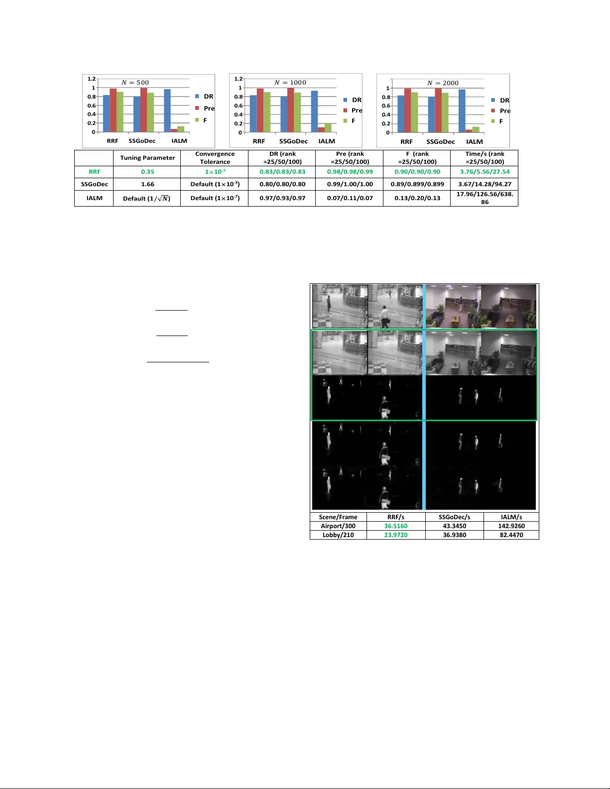
l 1 -r egularized Outlier Isolation and Regr ession Sheng Han Department of Electrical and Electronic Engineering, The Uni versity of Hong K ong, HKU Hong K ong, China sheng4151@gmail.com Suzhen W ang Department of Information Engineering, The Chinese Uni versity of Hong K ong, CUHK Hong K ong, China ws012@ie.cuhk.edu.hk Xinyu W u Shenzhen Institutes of Adv anced T echnology , CAS ShenZhen, China xy.wu@siat.ac.cn Abstract This paper pr oposed a new r e gression method called l 1 -r e gularized outlier isolation and r egr ession (LOIRE) as well as an efficient algorithm to solve it based on the idea of block coor dinate descent. Additionally , assuming out- liers ar e gr oss err ors following a Bernoulli pr ocess, this paper also pr oposed a Bernoulli estimate whic h, in theory , should be very accurate and r obust by completely remo v- ing every possible outliers. Howe ver , the Bernoulli estimate is not easy to achieve but with the help of the pr oposed LOIRE, it can be approximately solved with a guaranteed accuracy and an extr emely high ef ficiency compar ed to cur- r ent most popular r ob ust-estimation algorithms. Mor eover , LOIRE can be further extended to realize r obust rank fac- torization which is powerful in r ecovering low-r ank compo- nent fr om high corruptions. Extensive experimental r esults showed that the pr oposed method outperforms state-of-the- art methods like RPCA and GoDec in the aspect of compu- tation speed with a competitive performance. 1. Introduction Most rob ust estimates like least absolute de viate [9] real- ized by ADMM [3] and MM-estimator [5] are able to gi ve us accurate estimates but they are still computationally in- tensiv e which in a certain lev el prev ents these robust esti- mates from wide use. In this paper , we aimed to propose an efficient rob ust estimate called l 1 -regularized outlier isola- tion and regression, LOIRE in short, with a very parsimon y formulation. < ˆ x, ˆ b > = min x,b k b k 1 s.t. k y − Ax − b k 2 ≤ t, (1) where A denotes the measurement system, y denotes the measured data, x denotes the unknown signal to be deter- mined, b denotes the outlier vector and t to be a nonnegati ve value. In fact, LOIRE can be derived by assuming the noise is a mixture of Gaussian noise and Laplace noise. Howe ver , considered outliers are lar ge errors with a totally random oc- currence, it is more appropriate to assume their occurrences follow a Bernoulli process. With the ine vitable small oper- ation noises in the measurement system, we can e ventually deriv e a Bernoulli estimate as follows: < x 0 , b 0 > = min x,e k b k 0 s.t. k y − Ax − b k 2 ≤ t, (2) where < x 0 , b 0 > denotes the optimal solution pair under the Bernoulli assumption. Obviously , the Bernoulli estimate is difficult to solve and the LOIRE is less accurate. Fortunately , this paper found a way with a theoretical explanation in a certain lev el to achiev e an estimate which combines the Bernoulli esti- mate’ s accuracy with the LOIRE’ s efficienc y . Due to the parsimony and ef fecti veness of the LOIRE method, this paper further extended this method to realize robust rank factorization which can be applied to recover low-rank structures from massive contaminations, such as 4321 background modeling, face recognition and so on. Assum- ing that a data matrix Y ∈ R m × n consists of two parts: the lo w-rank part and the contamination part. Then to cor - rectly recover the low rank component equals to detect all the contaminations that can be treated as outliers. Below is the proposed robust f actorization model based on LOIRE: { ˆ A, ˆ X } = arg min A,X λ 2 k Y − AX − B k 2 2 + k B k 1 . s.t. k A · ,j k 2 = 1 , ∀ j = 1 , ..., n, (3) where matrix A ∈ R m × r can be understood as a dictionary which contains all the information about the low rank struc- ture, A · ,j indicates the j -th column of matrix A ∈ R m × r . Each column of X ∈ R r × n denotes a coef ficient vector for each column of Y . The products AX represents the low-rank component of Y while B reflects the contamina- tion component. Experiments both on simulation data and real image data would verify the high ef ficiency and strong robustness of this method compared to state-of-the-art ap- proaches like RPCA and GoDec. 2. Related W ork In robust statistics, least absolute deviations (LAD) re- gression [9] was proposed decades ago and has been used extensi vely in statistics but it lacks efficienc y especially when it comes to deal with large datasets. Recently , Boyd et al. [3] applied the ADMM algorithm to solve LAD fitting which greatly accelerate the computation speed, but it lacks stability and fluctuate its efficiency according to dif ferent dataset. Other popular robust regression methods with f ast implementations like fast-L TS [10], fast S-estimator [11], MM-estimator [5] and to name a few , are still facing the same problem of less efficiency , thus making them less practical to complicate real-life problems in a certain lev el. T o the best of the authors’ kno wledge, the most effec- tiv e low-rank recovery methods are [4, 13, 14], all of them combine strong rob ustness with high efficiency . For RPCA method [13], its fastest algorithm has been presented later in paper [7], which is called inexact ALM (IALM). For GoDec [14], it also published its fastened algorithm in [2], which is called SSGoDec. W e would show it later that the pro- posed rank factorization method based on LOIRE outper- forms these state-of-the-art methods in terms of efficiency with a competitiv e robustness. 3. l 1 -regularized Outlier Isolation and Regr es- sion In this paper, we consider a measurement system A which is has a probability p with p < 1 2 to be attacked by gross errors. T o be practical, we also need to consider the dense and normal operation noises besides the gross errors. So the measurement process can be expressed in a mathe- matical form: y = Ax + b + e (4) where y it the observ ation through A , b denotes the outlier vector and e denotes a dense Gaussian noise. By adding the penalty term k b k 1 to the least mean squares on e , we can e ventually deri ve an estimation model for x as follows: min e,b k e k 2 + µ k b k 1 s.t. µ > 0 , y = Ax + e + b, (5) which in fact has an equi v alent form as problem (1). 3.1. Alternativ e Direction Descent Algorithm for LOIRE In this subsection, we turn our attention to how to the LOIRE problem (1) which is con v ex but non-deriv ative. In truth, this problem can be re-formulated as: min x,b λ 2 k y − Ax − b k 2 2 + k b k 1 (6) with λ > 0 . Based on the idea of block coordinate descent, we can then deriv e an ef ficient algorithm for this problem. Firstly , fix b and optimize x only , we can get the first con vex subproblem: ˆ x = arg min x k y − Ax − b k 2 2 ; (7) and given A has full column rank, otherwise, we can apply Moore-Penrose pseudoin verse and then the solution for this sub-problem is: x = ( A T A ) − 1 A T ( y − b ) . (8) Fixed x and optimize b only , we can get the second conv ex subproblem: ˆ b = arg min b k b k 1 + λ 2 k y − Ax − b k 2 2 . (9) The second subproblem is essentially a lasso problem and paper [12] implies the solution as follows: < ˆ b i > = sig n (( y − Ax ) i )  | ( y − Ax ) i | − 1 λ  + . (10) Based on these above, we thus can giv e the alternati ve direction descent algorithm (ADD A) as shown in Algorithm 1. where ” ◦ ” is Hadamard product, i.e. entrywise produc- tion. The algorithm stops when b k +1 − b k <  for a gi ven small and positiv e  . 4322 Algorithm 1 Alternativ e Direction Descent Algorithm for LOIRE Require: The vector y and matrix A Ensure: 1: Initialization: b 0 = ~ 0 , k = 0 ; 2: while Not con ver gent do 3: x k +1 = ( A T A ) † A T ( y − b k ) . 4: let y k +1 = y − Ax k +1 . 5: b k +1 = sig n [ y k +1 ] ◦ h | y k +1 | − 1 λ ~ 1 i + 6: k = k+1 7: end while 8: return x, b 3.2. Conv ergence of ADD A In this subsection, we aim to show that the abov e algo- rithm will con ver ge to an optimal solution. First we sho wed the following sequence { ( x 0 , b 0 ) , ( x 1 , b 0 ) , ( x 1 , b 1 ) , ..., ( x k , b k − 1 ) , ( x k , b k ) , ... } (11) con verges to a fixed point, then we would show that this fixed point is actually an optimal solution for the LOIRE problem. Let f ( x, b ) = k b k 1 + λ 2 | y − Ax − b k 2 2 , (12) according to A V OM, we would hav e f ( x k , b k ) ≥ f ( x k +1 , b k ) ≥ f ( x k +1 , b k +1 ) ≥ ... > −∞ (13) , so this sequence must con ver ge to a certain fixed point denoted as ( x 0 , b 0 ) . Now we came to the second part of the proof: to show ( x 0 , b 0 ) is actually an optimal solution. From above, we could hav e: f ( x 0 + ∆ x, b 0 ) ≤ f ( x 0 , b 0 ) , f ( x 0 , b 0 + ∆ b ) ≤ f ( x 0 , b 0 ) . (14) Then for any conv ex combination of ( x 0 + ∆ x, b 0 ) and ( x 0 , b 0 + ∆ b ) , we should hav e: f ( x 0 + λ ∆ x, b 0 + (1 − λ )∆ b ) ≤ λf ( x 0 + ∆ x, b 0 ) + (1 − λ ) f ( x 0 , b 0 + ∆ b ) ≤ f ( x 0 , b 0 ) . (15) So ( x 0 , b 0 ) is actually a local optimal point but since f ( x, b ) is a con vex function, the local optimal point should also be a global one. Thus we finished our proof. 4. Bernoulli Estimation Model In this section, we aimed to arriv e at a Bernoulli estima- tion model (BEM) which is based on Bernoulli distribution assumption for outliers in the observations. 4.1. Notations Let I be an index set, then I c and |I | denote its com- plementary set and its cardinality respecti vely . Let X be a matrix (or a vector), then X I denotes a submatrix (vector) formed from the rows of X indexed by the elements in I . If I = { i } , the notation can be simplified as X i indicating the i -th row of X . 4.2. Bernoulli Estimation Model Let B ( p ) denote a Bernoulli distribution with an outlier appears with probability p . Let 1 denotes an outlier indica- tor of y : 1 i = 0 indicates that y i is a normal measurement, otherwise it is an outlier . If y i is an outlier with probability p then we can hav e 1 i ∼ B ( p ) : 1 i := ( 0 , p > 1 2 1 , 1 − p, (16) where p > 1 2 is a necessary guarantee to make a successful estimate. Let I be an index set of normal entries of y , that is ∀ i ∈ I , 1 i = 0 , then I c denotes the index set of outliers. In other words, we cay say I is an inde x set of normal mea- surements if and only if giv en a vector e ∈ R m satisfying k e k 2 ≤ t, (17) for some positiv e real number t , then y I = A I x + e I y i 6 = A i x + e i , ∀ i ∈ I c . (18) Obviously e ∈ R m reflects the acceptable noise in measure- ments. According to formula (18), we can hav e | I c | = k y − Ax − e k 0 , (19) with e satisfying condition (17). Gi ven a specific but un- known x , then according to the Bernoulli distribution, we can determine the probability for y with | I c | outlier entries: P ( y | x ) = p m −k y − Ax − e k 0 (1 − p ) k y − Ax − e k 0 . (20) Then apply the usual maximum log-likelihood method to the above formula, gi ven p > 1 2 , the Bernoulli estimation model is deriv ed as follows: < x 0 , e 0 > = min x,e k y − Ax − e k 0 s.t. k e k 2 ≤ t, (21) which has an equiv alent formula as follows: < x 0 , b 0 > = arg min x,b k b k 0 s.t. k y − Ax − b k 2 ≤ t. (22) Thus we obtained the BEM regression model. 4323 4.3. Relation between BEM and LMS Proposition 1 Assume ( x 0 , b 0 ) is the optimal solution of problem (22) and I is the support set of b 0 , then this optimal solution can be equally obtained by solving the following problem of least mean squares instead, i.e. Ax 0 = Ax 0 , where x 0 = arg min x k y I c − A T c x k 2 2 (23) The insight that this Proposition con veys to us is: if we can localize all the outliers in adv ance, then we can apply least mean squares estimation method to these uncorrupted mea- surements in order to get a Bernoulli estimation for x . The detailed mathematical proof is shown in the Appendices. 4.4. Approximate Bernoulli Estimate For LOIRE regression, it is ef ficient b ut it still suffers a slight deviation caused by outliers; for Bernoulli estimate, it is accurate but hard to compute. Fortunately , inspired by Proposition 1, there is simple way to combine the accu- racy of Bernoulli estimate with the ef ficiency of the LOIRE: firstly use LOIRE to detect the localization of the outliers; then remov e the entries corrupted by outliers in y ; Lastly apply the least mean squares on the cleaned observation. From Proposition 1, we can see, if LOIRE succeeds in detecting all the outliers, then the abov e steps w ould giv e a Bernoulli estimate. As for algorithm efficiency , the abov e process only append the ”least mean squares” step that is known to be fast to LOIRE, therefore, the abov e process is efficient and impro ves accuracy in a certain le vel. 5. Rank F actorization based on LOIRE Notations : for a matrix Y , let Y · ,i denote the i -th column of matrix Y . Generally , given a matrix Y ∈ R m × n with rank less than or equal to r , then it can be represented as a product of two matrices, Y = AX with A ∈ R m × r and X ∈ R r × n . Howe ver , in this section, we considered to recov er a lo w- rank component of a seriously contaminated matrix using a robust rank f actorization method based on LOIRE. Before we start the deri v ation of a ne w rob ust rank fac- torization model based on LOIRE, we should make the fol- lowing two things clear: one is each column of a contami- nated matrix Y should have equal chance to be corrupted; the other is the low-rank component of Y still can be appro- priately represented by AX . Below is the detailed deriv a- tion: First of all, assuming matrix A is known, we applied LOIRE to each column of Y : min B · ,i ,X · ,i k B · ,i k 1 + λ 2 k Y · ,i − AX · ,i − B · ,i k 2 2 , ∀ i = 1 , 2 , ..., n, (24) with B · ,i denotes an outlier vector for i -th column. T o be concise, we can re-represent formula (24) in the following form: min B ,X k B k 1 + λ 2 k Y − AX − B k 2 2 . (25) In fact, matrix A is generally unknown, then a simple way to find a most appropriate matrix A that fits the prob- lem is to search one that minimizes the abov e optimization problem. Thus the optimization problem becomes: min A min B ,X k B k 1 + λ 2 k Y − AX − B k 2 2 , (26) T o ensure a unique solution for matrix A and X , we would like to add a regularization constraint to matrix A , that is for each column of A , it should hav e a unit length: k A · ,j k 2 = 1 , ∀ i = 1 , ..., r. (27) Eventually , we got the proposed robust rank factorization model. 5.1. Algorithm f or Rob ust Rank Factorization After we deriv ed the robust rank f actorization model, we should come to focus on its solution algorithm. Similarly as ADD A, we can split the original problem into two subprob- lems: Fix matrix B , we can get the first subproblems: { A, X } = arg min A,X k Y − AX − B k 2 2 . s.t. k A · ,j k 2 = 1 . (28) Fix matrix A and X , we can get the second subproblem: { B } = arg min B k B k 1 + λ 2 k Y − AX − B k 2 2 . (29) The solution for the first subproblem is: A = U [1 : r ] , X = (Σ V T )(1 : r ) , (30) where ( Y − B ) = U Σ V T , i.e. the singular value decom- position with U [1 : r ] implies to take the first r columns of matrix U and (Σ V T )(1 : r ) takes the first r ro ws of matrix (Σ V T ) . The solution for the second subproblem is: B ij = sig n (( Y − AX ) ij )  | ( Y − AX ) ij | − 1 λ  + , (31) where B ij denotes an entry in the i -th ro w and j -th column of matrix B . Also similar to ADD A, we can deriv e an alternati ve ma- trix descent algorithm (AMD A) in Algorithm 2 to solve the robust rank factorization in algorithm. Follo wing the same line of the proof for ADD A, one can proof that AMD A will con verge to a global optimal solution. The AMDA algorithm stops if k B k +1 − B k k F ≤  giv en a small con vergence tolerance  > 0 . 4324 Algorithm 2 Alternative Matrix Descent Algorithm for Ro- bust Rank F actorization Require: Matrix Y Ensure: The matrix A , X , B 1: Initialization: k = 0 , B 0 = O ; 2: while Not con ver ged do 3: let ( Y − B k ) = U k Σ k V T k . 4: A k = U k [1 : r ] , X k = (Σ k V T k )(1 : r ) . 5: let Y k = Y − A k X k . 6: B k +1 = sig n [ Y k ] ◦  | Y k | − 1 λ 11 T  + 7: k = k + 1 ; 8: end while 9: return B , AX 6. Experiments The experiments is run by Matlab on a laptop with Intel i7 CPU (1.8G) and 8G RAM. All the reported results are direct outcomes of their corresponding algorithms without any post processing. 6.1. Appr oximate Bernoulli Estimate based on LOIRE In this part, we will compare the proposed rob ust regres- sion method with the most famous models in the area of robust regression. Algorithms chosen for each regression model to be compared to are all speeded up versions pro- posed in recent years. For LAD, we use ADMM proposed by Boyd et al. [3]; for S-estimation, we use the latest fas- tened algorithm proposed in paper [11]; for least-trimmed- squares re gression we use the latest fastened algorithm pro- posed in paper [10]; MM-estimation applied here is also a fastened algorithm proposed in [5]. W e conduct the com- parison experiments on data sets from [1]. Fig.1 sho ws that the approximate Bernoulli estimate holds the highest efficienc y with a competitive rob ustness. 6.2. Robust Rank Factorization 6.2.1 Simulations W e first demonstrate the performance of the proposed model on simulated data compared to GoDec and RPCA with their fastest implementations, SSGodec and IALM (in- exact ALM) respectiv ely . Inexact ALM [7] has much higher computation speed and higher precisions than previous al- gorithm for RPCA problem. SSGoDec [2] is also an im- prov ed version for GoDec [14], which largely reduces the time cost with the error non-increased. W ithout loss of generality , we can construct a square ma- trices of three different dimensions N = 500 , 1000 , 2000 and set rank r = 5% N . W e also need to generate three types of matrices for simulation, that is the lo w rank ma- trix L ∈ R N × N , the dense Gaussian noise matrix G ∈ ( a ) ( b ) ( c ) Figure 1. Comparison Experiment : Data in the top two graphs is cited from a public dataset [1]; Data in the bottom graph is cre- ated by authors with a dark line showing the ground truth. In (a), Lines of LOIRE, appBEM and MM-estimate overlap with each achiev es a very accurate estimate. The proposed LOIRE and appBEM achiev e the highest efficienc y . In (b), Lines of LOIRE and MM-estimate group together and the rest lines form a bunch. The proposed appBEM achiev es the highest efficiency with accu- racy . In (c) appBEM overlaps with the ground truth with a high efficienc y . R N × N , and the Bernoulli noise matrix B ∈ R N × N . L can be generated from a random matrix P = r and ( N , r ) by setting L = P P T , where r and ( N , r ) will generate a N × r random matrix. The Gaussian matrix can be set as G = 2 ∗ r and ( N , N ) with the coefficient indicat- ing its variance level. The Bernoulli matrix can be set as B = 10 ∗ spr and ( N , N , 5%) , where spr and ( N , N , 5%) will generate a sparse N × N random matrix with 5% indi- cating its sparse lev el. Experimental results will be ev aluated by using the fol- lowing three metrics: the detection rate (DR)/recall, the pre- 4325 T u n i n g Pa r a meter C o n v e r g e n c e T o l e r a n c e DR ( r a n k =2 5 / 5 0 / 1 0 0 ) Pr e ( r a n k = 2 5 / 5 0 / 1 0 0 ) F ( r a n k =2 5 / 5 0 / 1 0 0 ) T i me/ s ( r a n k =2 5 / 5 0 / 1 0 0 ) RRF 0 . 3 5 1 × 10 - 7 0 . 8 3 / 0 . 8 3 / 0 . 8 3 0 . 9 8 / 0 . 9 8 / 0 . 9 9 0 . 9 0 / 0 . 9 0 / 0 . 9 0 3 . 7 6 / 5 . 5 6 / 2 7 . 5 4 S S G o Dec 1 . 6 6 Def a u l t ( 1 × 10 - 3 ) 0 . 8 0 / 0 . 8 0 / 0 . 8 0 0 . 9 9 / 1 . 0 0 / 1 . 0 0 0 . 8 9 / 0 . 8 9 9 / 0 . 8 9 9 3 . 6 7 / 1 4 . 2 8 / 9 4 . 2 7 I AL M D e fa u l t ( 𝟏 / √ 𝑵 ) Def a u l t ( 1 × 10 - 7 ) 0 . 9 7 / 0 . 9 3 / 0 . 9 7 0 . 0 7 / 0 . 1 1 / 0 . 0 7 0 . 1 3 / 0 . 2 0 / 0 . 13 1 7 . 9 6 / 1 2 6 . 5 6 / 6 3 8 . 86 0 0 . 2 0 . 4 0 . 6 0 . 8 1 1 . 2 RRF S S G o D e c I A L M DR P r e F 0 0 . 2 0 . 4 0 . 6 0 . 8 1 RRF S S G o De c I A L M DR P r e F 0 0 . 2 0 . 4 0 . 6 0 . 8 1 1 . 2 RRF S S G o De c I A L M DR P r e F 𝑁 = 500 𝑁 = 1000 𝑁 = 2000 Figure 2. Simulation Results : T op: overall performance measured by detection rate (DR), precision (Pre) and F -measure under different matrix dimensions N . Both the proposed RRF and SSGoDec have the highest scores and IALM performs poor both in precision and F-measure. Bottom: presents the specific tuning parameter, con ver gence tolerance assigned to each model and its the corresponding DR, PRE, F-measure scores and the total computation time under different dimensions N . cision (Pre) and the F-measure (F) [8]: D R = tp tp + f n P r e = tp tp + f p F = 2 × D R × P r e D R + P r e (32) tp indicates the total number of corrupted pixels that are correctly detected; fn indicates the total number of cor- rupted pixels that are not being detected; fp denotes the total number of detected pixels which are actually normal. A good lo w-rank recov ery or a precise sparse-errors extrac- tion should hav e high detection rate, high precision and high F-measure. Among all the three metrics, F-measure is the most synthesized. The results are presented in Fig.2. The parameters are tuned for best performances. W e observed that the proposed robust rank factorization achieves very high scores of all the three metrics, which imply a very accurate reco very of low- rank matrices as well as a precise sparse-error detection. Meanwhile it pays the lowest time cost. 6.2.2 Backgr ound Modeling In this part, comparison experiments on real video data are conducted to further demonstrate the high computation ef- ficiency of the proposed rank factorization method. W e test the models on two video data from [6]: (1) airport (300 frames): there is no significant light changes in this video, but it has a lot of acti vities in the foreground. The image size is 144 × 176 ; (2) lobby (210 frames), there is little activity in this video, b ut it goes through significant illumi- nation changes. The image size is 128 × 160 . Fig. 3 shows that each model achie ves equally results and the proposed method remains to be the fastest among the three. S ce n e /F r a m e RRF /s S S G oD e c /s IA L M /s A i r port/ 300 36.5160 43.3450 142. 926 0 L obby /2 10 23.9720 36.9380 82.4470 Figure 3. Backgr ound Modeling : Left: airport scenario. Right: lobby scenario. The first row of the lar ge image presents two origi- nal frames of each video. The follo wing tw o ro ws inside the green box are extracted backgrounds and foregrounds by the proposed model. The last two rows are foregrounds extracted by SSGoDec and IALM respectiv ely . The table on the bottom gives the total running time of each model for each video. In a word, both the simulations and real-data experi- ments strongly v alidate the high computation ef ficiency and strong robustness of the the proposed model. 4326 7. Conclusion This paper presents a powerful regression method, LOIRE, which is efficient in detecting outliers and con- tributes a lot to approximately achiev e a Bernoulli estimate which is more accurate than LOIRE but with an almost equiv alent ef ficiency as LOIRE. Also, LOIRE can be fur- ther extended to realize a robust rank factorization which inherits the high ef ficiency of LOIRE and outperformed the state-of-the-art low-rank recovery methods, IALM and SS- GoDec both on simulations and on real-data experiments in terms of efficienc y with a competitive accurac y . A ppendices Proof of Proposition 1 First let at look at the following lemma: Lemma 1 : In problem (22), if ( x 0 , e 0 , b 0 ) is one of its optimal solution pair and I is a support set of b 0 , i.e. b i 6 = 0 for i ∈ I , then we should hav e e 0 i = 0 for i ∈ I . Pr oof of Lemma 1 : Let’ s consider another equiv alent form of problem (22) as follows: < x 0 , e 0 , b 0 > = arg min x,e λ 2 k e k 2 2 + k b k 0 s.t. e = y − Ax − b. (33) Suppose there ∃ k ∈ I such that e 0 k 6 = 0 , then we could construct another feasible pair ( b 0 , e 0 ) as below: ˜ b k = b 0 k + e 0 k , ˜ e k = 0 ˜ b − k = b 0 − k , ˜ e − k = e 0 − k , (34) where b − k indicates all the entries in b e xcept b k . It is ob- vious that k ˜ b k 0 ≤ k b 0 k . Since e 0 k 6 = 0 , then we must have k e 0 k k 2 > 0 and k b 0 k 0 + λ 2 k e 0 k 2 2 = k b 0 k 0 + λ 2 ( k e 0 − k k 2 2 + k e 0 k k 2 2 ) ≥ k ˜ b k 0 + λ 2 ( k e 0 − k k 2 2 + k e 0 k k 2 2 ) > k ˜ b k 0 + λ 2 ( k ˜ e k 2 2 ) , (35) which contradicts the optimality of feasible solution ( e 0 , b 0 ) . Then we prove the lemma.  Then we could continue on the proof for Proposition 1: It is obvious that k b 0 k 0 = k b 0 I k 0 . (36) According to Lemma 1, we should hav e e 0 I = y I − A I x 0 + b 0 I (37) According to the abov e two formula, we can ha ve k b 0 k 0 + λ 2 k y − Ax 0 − b 0 k 2 2 = k b 0 I k 0 + λ 2 k y I c − A I c x 0 k 2 2 (38) Since x 0 is an optimal solution for problem (22), then k b 0 I k 0 + λ 2 k y I c − A I c x 0 k 2 2 = min x {k b 0 k 0 + λ 2 k y − Ax − b 0 k 2 2 } = min x {k b 0 k 0 + λ 2 k y I c − A I c x k 2 2 + λ 2 k y I − A I x − b 0 I k 2 2 } ≥ k b 0 k 0 + λ 2 min x k y I c − A I c x k 2 2 k ˆ b k 0 + λ 2 k y − Ax − ˆ b k 2 2 w here ˆ b I c = 0 , ˆ b I = y I − A I x 0 ≥ min x,b k b k 0 + λ 2 k y − Ax − b k 2 2 (39) In the abov e inference, since the first ro w equals to the last row , therefore, all the ≥ should be replaced by = and hence we should hav e Ax 0 = Ax 0 .  References [1] The rousseeuw datasets, from:http://www .uni- koeln.de/themen/statistik/data/rousseeuw/. [2] Ssgodec, from:ttps://sites.google.com/site/godecomposition/code. [3] S. Boyd, N. Parikh, E. Chu, B. Peleato, and J. Eckstein. Distributed optimization and statistical learning via the al- ternating direction method of multipliers. F oundations and T rends R  in Machine Learning , 3(1):1–122, 2011. [4] E. J. Cand ` es, X. Li, Y . Ma, and J. Wright. Robust principal component analysis? Journal of the A CM (J A CM) , 58(3):11, 2011. [5] P . J. Huber . Robust Statistics . Springer , 2011. [6] L. Li, W . Huang, I. Y .-H. Gu, and Q. T ian. Statisti- cal modeling of complex backgrounds for foreground ob- ject detection. Ima ge Pr ocessing, IEEE T ransactions on , 13(11):1459–1472, 2004. [7] Z. Lin, M. Chen, and Y . Ma. The augmented lagrange mul- tiplier method for exact recovery of corrupted low-rank ma- trices. arXiv pr eprint arXiv:1009.5055 , 2010. [8] L. Maddalena and A. Petrosino. A fuzzy spatial coherence- based approach to background/foreground separation for moving object detection. Neural Computing and Applica- tions , 19(2):179–186, 2010. [9] J. L. Powell. Least absolute deviations estimation for the censored regression model. Journal of Econometrics , 25(3):303–325, 1984. 4327 [10] P . J. Rousseeuw and K. V an Driessen. Computing lts re- gression for large data sets. Data Mining and Knowledge Discovery , 12(1):29–45, 2006. [11] M. Salibian-Barrera and V . J. Y ohai. A fast algorithm for s- regression estimates. Journal of Computational and Graph- ical Statistics , 15(2), 2006. [12] R. T ibshirani. Regression shrinkage and selection via the lasso. Journal of the Royal Statistical Society , 58(1):267– 288, 1996. [13] J. Wright, A. Ganesh, S. Rao, Y . Peng, and Y . Ma. Robust principal component analysis: Exact recov ery of corrupted low-rank matrices via conv ex optimization. In Advances in neur al information pr ocessing systems , pages 2080–2088, 2009. [14] T . Zhou and D. T ao. Godec: Randomized low-rank & sparse matrix decomposition in noisy case. In Proceedings of the 28th International Conference on Mac hine Learning (ICML- 11) , pages 33–40, 2011. 4328