Estimating the Static Parameters in Linear Gaussian Multiple Target Tracking Models

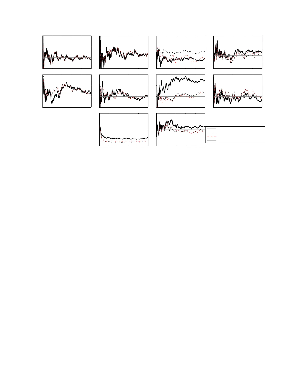
MANUSCRIPT SUBMITTED TO ARXIV .ORG, DECEMBER 2012 1 Estimating the Stati c Pa rameter s in Linea r Gaussian Multiple T ar get T racking Models Sinan Yıldırım a,b , Lan Jiang b , Sumeetpal S. Singh b , T om Dean Abstract —W e pres ent both ofﬂine and online maximum like- lihood estimation (MLE ) techniques f or inferring the static parameters of a multipl e tar get trackin g (MTT) model with linear Gaussian dynamics. W e present the b atch and online versions of the expectation-maximisation (EM) algorithm fo r short and long data sets respectiv ely , and we show how Monte Carlo approxima tions of these m ethods can be implemented. Perf ormance is assessed in numerical examples using simulated data fo r various scenarios and a comparison with a Bay esian estimation pr ocedure is also provided. I . I N T RO D U C T I O N The m ultiple target tracking (MTT ) prob lem concer ns the analysis of data from multiple movin g objects which are par- tially observed in noise to extract acc urate motion tra jectories. The M TT fr amew ork has b een tr aditionally ap plied to solve surveillance problems but more recently there has been a surge of interest in Bio logical Signal Processing, e.g. see [ 34]. The MTT framework is com prised o f th e f ollowing ingre- dients. A set of mu ltiple ind epende nt targets moving in the surveillance re gion in a Markov fashion. The number o f targets varies over tim e du e to departur e o f existing targets (known as death) and the arriv al of new targets ( known as birth ). The initial number o f targets are unknown and the maximum number of targets p resent a t a ny given time is unrestricted. At each time each target m ay genera te an observation which is a noisy record o f its state . T argets that do not generate ob serva- tions are said to be und etected a t that time. Additionally , the re may b e spu rious obser vations gener ated which a re un related to targets (kn own as clutter). The observation set at each time is the co llection of all target generated and false measur ements recorde d at that time, but without any information on the origin o r association of the m easurements. False m easure- ments, unknown o rigin of reco rded m easurements, undetected targets and a time varying number of targets rend er the task of extracting the motion trajecto ry of the und erlying ta rgets from the o bservation reco rd, which is known as tracking in the literature, a highly ch allenging problem . There is a large body of work o n the development of algorithm s for track ing multip le moving targets. Th ese al- gorithms ca n be categorised b y h ow they h andle the data association (or unkn own origin of record ed me asurements) a : Statisti cal Laboratory , Department of Pure Mathemati cs and Mathemat- ical Statisti cs, Uni ver sity of Cambridge, UK b : Department of E nginee ring, Univ ersity of Cambrid ge, UK L. Jiang, S.S. Singh and T . Dean’ s research is funded by the Engineerin g and Physical Scien ces Research Council (EP/G037590/1) whose support is gratefu lly ack no wledged. Some of the results in this work was presented by the authors in Yıldırım et al. [33] problem . Amo ng the main appro aches ar e the Multiple Hy- pothesis T r acking (MHT) algorith m [22] and the prob abilistic MHT (PMHT) variant [26], the joint pro babilistic da ta asso- ciation ﬁlter (JPDAF) [1, 2] , an d the prob ability hypo thesis density (PHD) ﬁlter [15, 24]. W ith the advancement of Monte Carlo methodolog y , sequential Monte Carlo (SMC) (or particle ﬁltering) and Markov cha in Monte Carlo (MCMC) meth ods have been applied to the MTT prob lem, e.g. SMC and MCMC implementatio ns of JPD A [14, 19], SMC implem entations of the MHT and PMHT [2 0, 27], a nd PHD ﬁlter [28, 29, 32]. Compared to th e hu ge amo unt of work on developing track- ing algo rithms, the pro blem of estimating the static par ameters of the tracking mo del has been largely neglected, altho ugh it is r arely the case that these param eters are known. Some exceptions include th e work o f Storlie et al. [25] where they extended the MHT algorithm to simu ltaneously estima te the parameters of th e MTT mo del. A fu ll Bayesian ap proach for estimating the mo del parameters using MCMC was presented in Y oon an d Singh [3 4]. Sing h et al. [23] presen ted an approx imated maximu m likeliho od method der iv ed by using a Poisson approx imation for the posterior distribution of the hidden targets which is also central to the deriv atio n of PHD ﬁlter in Mahler [15]. Add itionally , versions of PHD an d Cardinalised PHD (CPHD) ﬁlters that can learn the clutter rate and detection p roﬁle while ﬁltering are proposed in [16]. In this pap er , we p resent maximum likelihoo d estimation (MLE) algorithms to infer all the static parameter s of the MTT model when the ind ividual targets move accord ing to a linear Gaussian state-space mod el a nd when the tar get generated observations are linear f unctions of the target state corr upted with ad ditiv e Gaussian noise; we will hencefo rth call this a linear Gaussian MTT mo del. W e maxim ise the likeliho od function using the expectation- maximisation (E M) alg orithm and we pr esent both o nline and batch EM algorithm s. For a linear Gaussian MTT mo del we are able to present the exact recursions for updatin g static parameter estimate. T o th e best of ou r knowledge, this is a novel development in the target tracking ﬁeld. W e stress though th at th ese re cursions ar e n ot obvious by virtue of the m odel bein g linear Gaussian. This is because th e MTT mod el allo ws for false measu rements, unknown origin of rec orded m easuremen ts, undetected targets and a time varying number o f targets with unknown birth and death times. T o implemen t the pro posed EM algor ithms, an estimate of the po sterior distribution of the hidden targets giv en the o bservations is requ ired, and in the linear gau ssian setting, the con tinuous values of the target states c an be marginalised ou t. But, because the n umber of p ossible associ- ation of ob servations to targets g rows very quick ly with time, MANUSCRIPT SUBMITTED TO ARXIV .ORG, DECEMBER 2012 2 we ha ve to resort to appr oximation schem es that focu s the computatio n in the expectation (E)-step o f the EM algorithms on the most likely associations; that is, we app roximate the E-step with a Mo nte Carlo method . For this we employ both SMC an d MCMC which giv e rise to the following different MLE algorithms: • SMC-EM and MCMC-EM algorithm s for ofﬂine estima- tion; and • SMC online EM for o nline estimation. W e imp lement th ese three algorithms for simulated examples under v arious track ing scenarios an d p rovide reco mmend ations for the practitioner on wh ich one is to b e preferr ed. The EM alg orithms we present in this pap er can be imple- mented with any Monte-Carlo schem e f or in ferring the target states in MTT and reducing the errors in the appro ximation of th e E-step can on ly be ben eﬁcial to the EM p arameter estimates. W e do not f ully explore the use of th e v ario us Mo nte Carlo target track ing algorithm s that have been pro posed in the literature and instead focu s on the following two. When using SMC to app roximate the E-step, we compu te the L - best assignm ents [1 8] as the seq uential propo sal schem e of the particle ﬁlter . This L -best assignments appro ached ha s appeared previously in the literature in the context of track ing, e.g. see Cox and Miller [6], Danchick and Newnam [7], Ng et al. [19]. The MCMC algorith m we use for the E-step is th e MCMC-D A algor ithm propo sed for target tracking in Oh e t al. [20]. For further assessment/com parison of the EM alg orithms, we also implemen t a fu ll Bayesian estimation appro ach which is essentially a Gibb s like sampler for estimating the static parameters that alternates between sampling the target states and static param eter . No te that the Bayesian ap proach is not novel and a s it been prop osed by Y oon and Singh [ 34]. It is implemented in this work for the pu rpose of comp arison with the MLE techniques. The r emainder of the paper is organised as follows. In Section II, we describe the MTT mod el and formulate the static p arameter estimation problem . In Sectio n II I, w e pr esent the batch and online EM alg orithms. Section IV contains the numerical examples and we con clude the paper with a discussion o f our ﬁnd ings in Sectio n V. Th e Appendix contains furthe r details on the derivation o f the MTT EM algorithm , and details of the SMC and MCMC alg orithms we use in this p aper . A. Notatio n W e in troduce r andom variables (also sets and mapp ings) with capital letters such as X, Y , Z, X , A and de note th eir realisations by co rrespon ding small case letters x, y , z , x , a . If a non-discrete r andom variable X has a density ν ( x ) , with all densities being deﬁned w .r .t. th e L ebesgue measure (deno ted by dx ), we write X ∼ ν ( · ) to make explicit the law of X . W e use E θ [ ·|· ] for the (cond itional) expec tation operator ; for jointly distributed rando m variables X, Y and Z a nd a fu nction ( x, z ) → f ( x, z ) , E θ [ f ( X , Z ) | Y = y ] is the expec tation of the random variable f ( X , Z ) w .r .t. the joint distribution of X , Z condition ed o n Y = y . E θ [ f ( X , z ) | y ] is the expectation of the function x → f ( x, z ) for a ﬁxed z given Y = y . I I . M U LT I P L E TA R G E T T R A C K I N G M O D E L Consider ﬁrst a single target tracking mo del where a moving object (or target) is ob served when it traverses in a surveillance region. W e deﬁn e the target state an d the n oisy obser vation at time t to be the ran dom variables X t ∈ X ⊂ R d x and Y t ∈ Y ⊂ R d y respectively . The statistical mo del mo st common ly used f or the evolution of a target and its observa- tions { X t , Y t } t ≥ 1 is the hidd en Markov model (HMM). I n a HMM, it is assume d tha t { X t } t ≥ 1 is a hidd en Markov pr ocess with initial and transition probability den sities µ ψ and f ψ , respectively , and { Y t } t ≥ 1 is the observation process with the condition al observation d ensity g ψ , i.e. X 1 ∼ µ ψ ( · ) , X t | ( X 1: t − 1 = x 1: t − 1 ) ∼ f ψ ( ·| x t − 1 ) Y t |  { X i = x i } i ≥ 1 , { Y i = y i } i 6 = t  ∼ g ψ ( ·| x t ) . (1) Here the densities µ ψ , f ψ and g ψ are par ametrised by a r eal valued vector ψ ∈ Ψ ⊂ R d ψ . In this paper, we co nsider a speciﬁc type o f HMM, the Gaussian linear state-space model (GLSSM), which can be speciﬁed as µ ψ ( x ) = N ( x ; µ b , Σ b ) , f ψ ( x ′ | x ) = N ( x ′ ; F x, W ) , g ψ ( y | x ) = N ( y ; Gx, V ) . (2) where N ( x ; µ, Σ) denotes the probab ility density function for the multiv aria te normal distribution with mean µ and covariance Σ . In th is case, ψ = ( µ b , Σ b , F, G, W , V ) . In a M TT mo del, the state and the observation at each time ( t ≥ 1 ) are random ﬁnite sets, X t =  X t, 1 , X t, 2 , . . . , X t,K x t  and Y t =  Y t, 1 , Y t, 2 , . . . , Y t,K y t  . Here eac h element of X t is the state of an in dividual target an d elem ents of Y t are the distinct measur ements of these targets at time t . The nu mber of targets K x t under surveillance changes over time due to targets entering an d leaving the sur veillance region X . X t ev olves to X t +1 as follows: with p robab ility p s each target X t ‘survives’ and is displaced according to the state transition density f ψ in (2), oth erwise it dies. The random d eletion a nd Markov mo tion h appens independe ntly f or all the elements of X t . In ad dition to the survi ving targets, ne w targets are created. The n umber of new targets created p er time follows a Poisson distribution with m ean λ b and each of their states is in itiated indepen dently according to the initial den sity µ ψ in (2). Now X t +1 is deﬁned to be the super position of the states o f the surviving and e volved targets from time t and the newly born targets at time t +1 . The elements o f X t are observed throu gh a process of ran dom thinning and disp lacement: with pro bability p d , each point of X t generates a noisy o bservation in the observation space Y th rough the observation density g ψ in (2 ). This hap pens indep endently for each poin t of X t . In addition to these target g enerated o bservations, false measuremen ts are also gen erated. The nu mber of false m easuremen ts collected at each time follows a Po isson distribution with mea n λ f and their values are un iform over Y . Y t is the superp osition o f observations origin ating from the detected targets and these false measurements. A series of ran dom variables, wh ich are essential for the statistical analysis to follow are now deﬁned . Let C s t be a K x t − 1 × 1 vector of 1 ’ s and 0 ’ s where 1 ’ s indicate sur viv als MANUSCRIPT SUBMITTED TO ARXIV .ORG, DECEMBER 2012 3 and 0 ’ s in dicate dea ths o f targets fro m time t − 1 . For i = 1 , . . . , K x t − 1 , C s t ( i ) = ( 1 i ’th target at time t − 1 surviv es to time t 0 i ’th target at time t − 1 does n ot surviv e to t . The number o f sur viving targets at time t is K s t = P K x t − 1 i =1 C s t ( i ) . W e also deﬁne the K s t × 1 vector I s t containing the indices of surviving targets a t time t , I s t ( i ) = min    k : k X j =1 C s t ( j ) = i    , i = 1 , . . . , K s t . Note that I s t ( i ) will also denote the ancestor o f target i f rom time t − 1 , i.e. X t − 1 ,I s t ( i ) ev olves to X t,i for i = 1 , . . . , K s t . Denoting the n umber of ‘births’ at time n as K b t , we h av e K x t = K s t + K b t . Note that acco rding to these deﬁnitions, the su rviving targets from time t − 1 are re- labeled as X t, 1 , . . . , X t,K s t , and the newly b orn targets are denoted as X t,K s t +1 , . . . , X t,K x t . Next, g iv en K x t targets we d eﬁne C d t to be a K x t × 1 vector of 1 ’ s an d 0 ’ s where 1 ’ s in dicate d etections and 0 ’ s indicate non-de tections. For i = 1 , . . . , K x t , C d t ( i ) = ( 1 i ’th target at time t is detected at time t, 0 i ’th target at time t is not detected at time t. , Therefo re, the num ber o f detected targets at time t is K d t = P K x t i =1 C d t ( i ) . Similarly , we also deﬁne the K d t × 1 vector I d t showing the indices of the detected targets, I d t ( i ) = min    k : k X j =1 C d t ( j ) = i    , i = 1 , . . . , K d t . I d t ( i ) denotes the label o f the i -th detected target at time t . So the detected targets at time t are X t,I d t (1) , . . . , X t,I d t ( K d t ) . Finally , deﬁning th e num ber of false measurements at time t as K f t , we ha ve K y t = K d t + K f t and the associatio n from th e detected targets to th e observations c an be represented by a one-to- one mapp ing A t : { 1 , . . . , K d t } → { 1 , . . . , K y t } where at time t the i ’th detected target is target I d t ( i ) with state value X t,I d t ( i ) and generates Y t,A t ( i ) . W e assume tha t A t is uniform over the set of all K y t ! /K f t ! possible one-to - one mapp ings. T o summ arise, we giv e the list of the random variables in the MTT model introdu ced in this section as well as a sample r ealisation of them in Fig ure 1. The main d ifﬁculty in an M TT prob lem is that in general we do not know b irth-death times of targets, wheth er th ey are d etected o r no t, and which o bservation point in Y t is associated to which detected target in X t . Let Z t =  C s t , C d t , K b t , K f t , A t  be the collection of the just m entioned un known random variables at time t , and θ = ( ψ , p s , p d , λ b , λ f ) ∈ Θ = Ψ × [0 , 1] 2 × [0 , ∞ ) 2 be th e vector o f the MTT m odel para meters. W e can write the joint likeliho od of all the ran dom variables of the MTT model up to time n g iv en θ as p θ ( z 1: n , x 1: n , y 1: n ) = p θ ( z 1: n ) p θ ( x 1: n | z 1: n ) p θ ( y 1: n | x 1: n , z 1: n ) where p θ ( z 1: n ) = n Y t =1 p k s t s (1 − p s ) k x t − 1 − k s t P O ( k b t ; λ b ) p k d t d (1 − p d ) k x t − k d t P O ( k f t ; λ f ) k f t ! k y t ! ! (3) p θ ( x 1: n | z 1: n ) = n Y t =1   k s t Y j =1 f ψ ( x t,j | x t − 1 ,i s t ( j ) ) k x t Y j = k s t +1 µ ψ ( x t,j )   (4) p θ ( y 1: n | x 1: n , z 1: n ) = n Y t =1   |Y | − k f t k d t Y j =1 g ψ ( y t,a t ( j ) | x t,i d t ( j ) )   (5) Here P O ( k ; λ ) denotes the prob ability mass fun ction of th e Poisson d istribution with mean λ , |Y | is the volume (w .r . t. the Lebesgu e measure) of Y and the term k f t ! /k y t ! in (3) correspo nds to the law of A t . The marginal likeliho od o f the observation sequenc e y 1: n is p θ ( y 1: n ) = E θ [ p θ ( y 1: n | X 1: n , Z 1: n )] . (6) The m ain aim of this paper is, given Y 1: n = y 1: n , to estimate the static parameter θ ∗ where we assume the d ata is g enerated by some true but unkn own θ ∗ ∈ Θ . Our main con tribution is to present the EM algorithms, both batch and online versions, for computin g the MLE of θ ∗ : θ ML = arg max θ ∈ Θ p θ ( y 1: n ) . For comp arison sake we a lso present the Bay esian estimate of θ ∗ . In the Bay esian ap proach, the static p arameter is treated as random variable tak ing values θ in Θ with a pr obability density η ( θ ) and the a im is to ev a luate the den sity of the posterior distribution of θ given y 1: n , i.e. p ( θ | y 1: n ) = η ( θ ) p θ ( y 1: n ) R Θ η ( θ ) p θ ( y 1: n ) dθ . Y oon and Sin gh [34] use MCMC to sample from p ( θ | y 1: n ) which integrates both Metrop olis-Hastings a nd Gibbs moves. I I I . E M A L G O R I T H M S F O R M T T In this sectio n we present the batch and online EM al- gorithms f or lin ear Gaussian MTT mo dels. Th e no tation is in volved and we provide a list of the importan t variables used in the deriv ation of the EM algorithms in T able I at the end of the section. A. Ba tch EM for MTT Giv en Y 1: n = y 1: n , the EM algo rithm for maximising p θ ( y 1: n ) in (6) is g iv en by the fo llowing iterati ve p rocedu re: if θ j is the estimate of the EM alg orithm at the j ’th iteratio n, then at iteratio n j + 1 the estimate is updated by ﬁrst calculating the MANUSCRIPT SUBMITTED TO ARXIV .ORG, DECEMBER 2012 4 Complete li st of random v ariables of the MTT model X t,k , Y t,k : k ’th target and k ’th observ ation at time t . X t = { X 1 , . . . , X K x t } , Y t = { Y t, 1 , . . . , Y t,K y t } : Sets of targets and observ ations at time t . K b t , K f t : Numbers of ne w born targets and false measurements at t ime t K s t , K d t : Numbers of targets surviv ed from time t − 1 to time t and detected at time t . K x t , K y t : Numbers of aliv e targ ets and observ ations at time t . K x t = K s t + K b t , K y t = K d t + K f t . C s t : K x t − 1 × 1 v ector of 0 ’ s and 1 ’ s indicating survi ving targets from time t − 1 to time t . C d t : K x t × 1 vector of 0 ’ s and 1 ’ s indicating detected targets at time t . I s t : K s t × 1 vector of labels of survi ving targets from time t − 1 to time t . I d t : K d t × 1 vector of labels of detected targ ets at time t . A t : { 1 , . . . , K d t } → { 1 , . . . , K y t } : Association from detected targets to observations at time t . X 1 , 1 X 2 , 1 X 3 , 1 X 4 , 1 X 5 , 1 Y 1 , 4 Y 3 , 3 Y 5 , 3 X 1 , 2 X 2 , 2 X 3 , 2 X 4 , 2 X 5 , 2 Y 1 , 1 Y 2 , 1 Y 3 , 5 Y 4 , 1 Y 5 , 2 X 1 , 3 X 2 , 3 X 3 , 3 X 4 , 3 X 5 , 3 Y 1 , 2 Y 2 , 3 Y 3 , 4 Y 4 , 2 Y 5 , 1 Y 1 , 3 X 2 , 4 Y 3 , 1 X 4 , 4 X 5 , 4 Y 1 , 5 Y 2 , 2 Y 3 , 2 Y 4 , 3 Y 5 , 4 Fig. 1. T op: Complete list of the discrete random v ariables of the MTT model. B ottom: A realisat ion from MTT model: States of a tar gets are connecte d with arro ws and with its observ ations when detected. Undetected targets highli ghted w ith shado ws , and false mea- surements are coloured grey . C s 1:5 = ([ ] , [1 , 1 , 1] , [1 , 0 , 1 , 1] , [0 , 1 , 1] , [1 , 1 , 1 , 1]) ; I s 1:5 = ([ ] , [ 1 , 2 , 3] , [1 , 3 , 4] , [2 , 3] , [1 , 2 , 3 , 4]) ; C d 1:5 = ([1 , 1 , 0] , [0 , 1 , 1 , 1] , [1 , 1 , 1] , [ 0 , 1 , 1 , 0] , [1 , 1 , 1 , 1]) ; I d 1:5 = ([1 , 2] , [2 , 3 , 4] , [1 , 2 , 3] , [ 2 , 3] , [1 , 2 , 3 , 4]) ; K s 1:5 = (0 , 3 , 3 , 2 , 4) ; K b 1:5 = (3 , 1 , 0 , 2 , 0) ; K d 1:5 = (2 , 3 , 3 , 2 , 4) ; K f 1:5 = (3 , 0 , 2 , 1 , 0) , A 1:5 = ([4 , 1] , [1 , 3 , 2] , [3 , 5 , 4] , [1 , 2] , [3 , 2 , 1 , 4]) . following interm ediate o ptimisation criterion, which is known as the expectation (E) step, Q ( θ j , θ ) = E θ j [log p θ ( X 1: n , Z 1: n , y 1: n ) | y 1: n ] = E θ j [log p θ ( Z 1: n ) + log p θ ( X 1: n , y 1: n | Z 1: n ) | y 1: n ] = E θ j [log p θ ( Z 1: n ) + E θ j { log p θ ( X 1: n , y 1: n | Z 1: n ) | y 1: n , Z 1: n } | y 1: n  (7) The updated estimate is then co mputed in the maximisation (M) step θ j +1 = arg max θ ∈ Θ Q ( θ j , θ ) This proced ure is repeated until θ j conv erges (or in pra ctice ceases to change signiﬁcantly ). From equ ations (2)-(5), it can be shown that the E -step at the j ’th iteration redu ces to calculating th e expectatio ns of ﬁfteen sufﬁcient statistics of x 1: n , z 1: n and y 1: n denoted by S 1 ,n , . . . , S 15 ,n . (Fr om now on, any depen dancy on y 1: n in these sufﬁcient statistics and further variables arising from th em will be omitted fro m the notation for simplicity .) Sufﬁcient statistics S 1 ,n ( x 1: n , z 1: n ) to S 7 ,n ( x 1: n , z 1: n ) are: n X t =1 k d t X k =1 x t,i d t ( k ) x T t,i d t ( k ) , n X t =1 k d t X k =1 x t,i d t ( k ) y T t,a t ( k ) , n X t =2 k s t X k =1 x t − 1 ,i s t ( k ) x T t − 1 ,i s t ( k ) , n X t =2 k s t X k =1 x t,k x T t,k , (8) n X t =2 k s t X k =1 x t − 1 ,i s t ( k ) x T t,k , n X t =1 k x t X k = k s t +1 x t,k , n X t =1 k x t X k = k s t +1 x t,k x T t,k These sufﬁcient statistics are r elated to those used for es- timating the static p arameters of a linear Gau ssian single target track ing mod el, and this relation will be made more explicit later . The r est o f the sufﬁcient statistics S 8 ,n ( z 1: n ) to S 15 ,n ( z 1: n ) do not d epend on x 1: n . [ S 8 ,n , . . . , S 15 ,n ] ( z 1: n ) = n X t =1   k d t X k =1 y t,a t ( k ) y T t,a t ( k ) , k d t , k x t , k s t , k x t − 1 , k b t , k f t , 1   (9) Let S θ m,n denote the expectation o f th e m ’th sufﬁcient statistic w .r .t. the law of the latent variables X 1: n and Z 1: n condition al MANUSCRIPT SUBMITTED TO ARXIV .ORG, DECEMBER 2012 5 upon the observation y 1: n for a giv en θ , i.e. S θ m,n = ( E θ [ S m,n ( X 1: n , Z 1: n ) | y 1: n ] 1 ≤ m ≤ 7 , E θ [ S m,n ( Z 1: n ) | y 1: n ] 8 ≤ m ≤ 15 . (10) Then the solu tion to the M-step is g iv en by a kn own function Λ :  S θ 1 ,n , . . . , S θ 15 ,n  → Θ such that at iteration j θ j +1 = arg max θ Q ( θ j , θ ) = Λ  S θ j 1 ,n , . . . , S θ j 15 ,n  . The explicit expression of Λ dep ends on the pa rametrisation of the MTT mod el, in particular on the parametrisation of the matrices F, G, W , V , µ b , Σ b as in the f ollowing example. Example 1. (The constant velocity model:) Each tar get has a position and velocity in th e xy -plan e an d hence X t = [ X t (1) , X t (2) , X t (3) , X t (4)] T ∈ X = R 2 × [0 , ∞ ) 2 , wher e X t (1) , X t (2) ar e the x and y coordinates an d X t (3) , X t (4) ar e the ve locities in x and y d ir ection s. On ly a no isy measurement of the position of the target is availab le [ Y t (1) , Y t (2)] ∈ Y = [ − κ, κ ] 2 . W e assumed a bo unded Y and r egar d ob servations that ar e no t r eco r d ed due to being outside this interval as also a missed detection. W ith r efer en ce to (2) , the single tar get state-space model is µ b = [ µ bx , µ by , 0 , 0] T , Σ b =  σ 2 bp I 2 × 2 0 2 × 2 0 2 × 2 σ 2 bv I 2 × 2  F =  I 2 × 2 ∆ I 2 × 2 0 2 × 2 I 2 × 2  , G =  I 2 × 2 0 2 × 2  W =  σ 2 xp I 2 × 2 0 2 × 2 0 2 × 2 σ 2 xv I 2 × 2  , V = σ 2 y I 2 × 2 Ther e for e, the parameter vector of this MTT model is θ =  λ b , λ f , p d , p s , µ bp , µ bv , σ 2 bp , σ 2 bv , σ 2 xp , σ 2 xv , σ 2 y  . The upda te rule Λ for θ at the M-step of the EM algo rithm is µ bx = S θ 6 ,n (1) /S θ 13 ,n , µ by = S θ 6 ,n (2) /S θ 13 ,n , σ 2 bp = 1 2 S θ 13 ,n tr  S θ 7 ,n − 2 S θ 6 ,n µ T b + S θ 13 ,n µ b µ T b  M T p M p  σ 2 bv = 1 2 S θ 13 ,n tr  S θ 7 ,n − 2 S θ 6 ,n µ T b + S θ 13 ,n µ b µ T b  M T v M v  σ 2 xp = tr  S θ 4 ,n M T p M p − 2 S θ 5 ,n M p F p + S θ 3 ,n F T p F p  / 2 S θ 11 ,n , σ 2 xv = tr  S θ 4 ,n M T v M v − 2 S θ 5 ,n M v F v + S θ 3 ,n F T v F v  / 2 S θ 11 ,n , σ 2 y = tr  S θ 8 ,n − 2 GS θ 2 ,n + GS θ 1 ,n G T  / 2 S θ 9 ,n , p d = S θ 9 ,n /S θ 10 ,n , p s = S θ 11 ,n /S θ 12 ,n , λ b = S θ 13 ,n /S θ 15 ,n , λ f = S θ 14 ,n /S θ 15 ,n , wher e M p =  I 2 × 2 0 2 × 2  , M v =  0 2 × 2 I 2 × 2  , and F p and F v ar e the u pper an d lower halve s of F , that is F p ( i, j ) = F ( i, j ) and F v ( i, j ) = F (2 + i, j ) for i = 1 , 2 and j = 1 , . . . , 4 . 1) Estimation of sufﬁcient statistics: It is easy to calculate the expe ctation of the su fﬁcient statistics in ( 9) that do not depend on x 1: n . Noting that Z t is discrete, we simply calculate S m,n ( z 1: n ) for every z 1: n with a positive mass w .r . t. to the density p θ ( z 1: n | y 1: n ) and calculate the expectatio ns as S θ m,n = X z 1: n S m,n ( z 1: n ) p θ ( z 1: n | y 1: n ) . For those sufﬁcient statistics in ( 8) that d epend o n x 1: n , con- sider the last expression in (7) with the following facto risation of the posterior p θ ( x 1: n , z 1: n | y 1: n ) = p θ ( x 1: n | z 1: n , y 1: n ) p θ ( z 1: n | y 1: n ) . This factorisation sugg ests that we can write the required expectations as S θ m,n = E θ [ S m,n ( X 1: n , Z 1: n ) | y 1: n ] = E θ [ E θ [ S m,n ( X 1: n , Z 1: n ) | Z 1: n , y 1: n ] | y 1: n ] . (11) Let u s deﬁne the integrand of the outer expe ctation in (11) which is the conditional expectatio n e S θ m,n ( z 1: n ) = E θ [ S m,n ( X 1: n , z 1: n ) | z 1: n , y 1: n ] . as a matrix-valued fun ction with d omain Z n . Then, we can obtain S θ m,n by calculatin g e S θ m,n ( z 1: n ) for ev ery z 1: n with a positive m ass w .r . t. the density p θ ( z 1: n | y 1: n ) a nd then calcu late S θ m,n = X z 1: n e S θ m,n ( z 1: n ) p θ ( z 1: n | y 1: n ) . The cru cial point here is th at it is possible to calculate e S θ m,n ( z 1: n ) for any given z 1: n . In fact, the a vailability of this calculatio n is based on the f ollowing fact: cond itional on { Z t } t ≥ 1 , { X t , Y t } t ≥ 1 may be r egar ded as a collectio n of indepen dent GLSS Ms (with dif fer en t starting and en ding times, possible missing observation s) and ob servations which ar e not r elevant to any of these GLSSMs . In the context o f MTT , each GLSSM correspond s to a target a nd ir relev a nt observations correspo nd to false measur ements. W e defer details on h ow e S θ m,n ( z 1: n ) is calculated to Section III-B. 2) Stochastic versions of EM: For exact calculation of th e E-step of the EM algorithm we need p θ ( z 1: n | y 1: n ) which is infeasible to calculate due to the h uge cardinality of Z n . W e thus resort to Monte Carlo approxim ations of p θ ( z 1: n | y 1: n ) which we then use in the E-step ; in litera ture this appro ach is g enerically known as th e stoch astic EM algorithm [5, 9, 31]). W e know from the previous sections th at given Z 1: n = z 1: n the po sterior distribution p θ ( x 1: n | y 1: n , z 1: n ) is Gaussian and condition al expectations can b e e valuated. Ther efore, it is sufﬁcient to have the Mon te Carlo pa rticle approx imation for p θ ( z 1: n | y 1: n ) only , wh ich is expr essed as b p θ ( z 1: n | y 1: n ) = N X i =1 w ( i ) n δ z ( i ) 1: n ( z 1: n ) , N X i =1 w ( i ) n = 1 . (12) Then, th e co rrespond ing par ticle app roximatio ns fo r the ex- pectations of the su fﬁcient statistics are b S θ m,n = ( P N i =1 w ( i ) n e S θ m,n ( z ( i ) 1: n ) , 1 ≤ m ≤ 7 , P N i =1 w ( i ) n S m,n ( z ( i ) 1: n ) , 8 ≤ m ≤ 15 . MANUSCRIPT SUBMITTED TO ARXIV .ORG, DECEMBER 2012 6 When θ changes with each EM iteration, the appro priate update schem e at iteration j in volves a stochastic app roxima- tion procedur e where in the E-step one c alculates a weighted av erage of b S θ 1 m,n , . . . , b S θ j m,n ; the resultin g algorithm is known as th e stocha stic ap proxim ation EM (SAEM) [ 9]. Speciﬁcally , let γ = { γ j } j ≥ 1 , ca lled the step-size sequence, be a p ositiv e decreasing sequence satisfying X j γ j = ∞ , X j γ 2 j < ∞ . A comm on ch oice is γ j = j − α for 0 . 5 < α ≤ 1 . The SAEM algorithm is gi ven in Algor ithm 1 . Algorithm 1. The SAEM algorithm for the MTT model Start with θ 1 and b S (0) γ ,m,n = 0 for m = 1 , . . . , 15 . F or j = 1 , 2 , . . . • E-step: Calculate b S θ j m,n for each m , and t hen calculate the weighted avera ges b S ( j ) γ ,m,n = (1 − γ j ) b S ( j − 1) γ ,m,n + γ j b S θ j m,n . (13) • M-step Update the parameter esti mate using Λ( · ) as befor e θ j +1 = Λ  b S ( j ) γ , 1 ,n , . . . , b S ( j ) γ , 15 ,n  . In general, the Monte Carlo appro ximation b p θ j ( z 1: n | y 1: n ) in (1 3) is perfor med either sampling N samples from p θ j ( z 1: n | y 1: n ) using a MCMC m ethod (in which case weights w ( i ) n = 1 / N , i = 1 , . . . , N ) or using a SMC method with N particles. Dependin g o n which method is used , we will call the r esulting algo rithm MCMC-EM or SMC-EM, respectively . For MCMC, we use the MCMC-DA algorithm of [20], but with so me reﬁn ements of the MCMC proposals. (Details are av ailable from the author s.) W e use SMC to obtain the app roximatio ns { b p θ ( z 1: t | y 1: t ) } 1 ≤ t ≤ n sequentially as follows. Assume that we ha ve the ap proxim ation at time t − 1 b p θ ( z 1: t − 1 | y 1: t − 1 ) = N X i =1 w ( i ) t − 1 δ z ( i ) 1: t − 1 ( z 1: t − 1 ) . T o av oid weigh t degener acy , at ea ch time one can resample from b p θ ( z 1: t − 1 | y 1: t − 1 ) to obtain a new collection of N particles an d th en p roceed to the time t . Alternatively , this resampling operatio n can be do ne according to a criterion which measur es the weight degener acy (e.g . see Douc et et al. [11]). W e deﬁne the N × 1 random m apping Π t : { 1 , . . . , N } → { 1 , . . . , N } containing the ind ices of the resampled particles, i.e. Π t ( i ) = j if the i ’th resampled particle is z ( j ) 1: t − 1 . (I f no r esampling is perfor med at the end of time t − 1 , th en Π t ( i ) = i fo r all i .) Th en, given y t and Π t = π t , the particle z ( i ) t at time t is sampled from a proposal d istribution q θ  z t    z ( π t ( i )) 1: t − 1 , y 1: t  for i = 1 , . . . , N . There fore, z ( i ) t is con nected to z ( π t ( i )) 1: t − 1 and the i ’th path particle at time t is z ( i ) 1: t = ( z ( i ) t , z ( π t ( i )) 1: t − 1 ) and its new weight is w ( i ) t ∝ ¯ w ( π t ( i )) t − 1 × p θ ( z ( i ) t | z ( π t ( i )) t − 1 ) p θ ( y t | y 1: t − 1 , z ( i ) 1: t ) q θ ( z ( i ) t | z ( π t ( i )) 1: t − 1 , y 1: t ) (14) where, for i = 1 , . . . , N , we take ¯ w ( i ) t − 1 = 1 / N if resampling is performed and ¯ w ( i ) t − 1 = w ( i ) t − 1 otherwise. Note tha t we also need to imp lement SMC for the online EM algorith m in ord er to ob tain a Monte Carlo appr oximation of th e E-step. Our SMC alg orithm ca lculates the L -b est linear assignments [18] as the seque ntial propo sal; see Appen dix B for details. B. On line EM fo r MTT W e showed in the previous section how to im plement the batch E M algorithm f or M TT using Monte Carlo appro xima- tions. However , the batch E M algo rithm is computationally demand ing when the data sequence y 1: n is long since one iteration of the EM requ ires a comp lete br owse of the data. In these situations, the online version of the EM algorithm which up dates the p arameter estimates as a new d ata reco rd is received at each time can b e a m uch cheaper alter native. In this section, we p resent a SMC online EM algorithm for linear Gaussian MTT models. An important observation at this point is that the sufﬁcient statistics of interest for the EM algo rithm have a certain additive f orm such th at the d ifference of S m,n ( x 1: n , z 1: n ) and S m,n − 1 ( x 1: n − 1 , z 1: n − 1 ) o nly depends o n ( x n − 1 , x n , y n ) . This enables us to com pute the required expectations in the E-step of the EM algor ithm e ffecti vely in an online manner . W e shall see in th is section that, with a ﬁxed amo unt of com putation and memory pe r time, it is p ossible to update f rom e S θ m,t − 1 ( z 1: t − 1 ) to e S θ m,t ( z 1: t ) given y t and z t at time t . T o show how to hand le the sufﬁcient statistics in (8) for the MTT m odel, we ﬁrst start with a single GLSSM and then extend the idea to the MTT case by showing the relation between the sufﬁcient statistics in a single GLSSM and in the MTT mod el. 1) Online smoothing in a single GLSS M: Consider the HMM { X t , Y t } t ≥ 1 deﬁned in (1). I t is possible to ev aluate expectations o f additiv e fun ctionals o f X 1: n of the form S n ( x 1: n ) = s ( x 1 ) + n X t =2 s ( x t − 1 , x t ) (with possible depend ancy on y 1: n also allowed) w .r .t. the posterior density p θ ( x 1: n | y 1: n ) in an on line mann er using only the ﬁlterin g densities { p θ ( x t | y 1: t ) } 1 ≤ t ≤ n . The technique is based on the following recursion on the inter mediate function [4, 8] T θ t ( x t ) := E θ [ S t ( X 1: t ) | X t = x t , y 1: t ] = E θ  T θ t − 1 ( X t − 1 ) + s ( X t − 1 , x t )   y 1: t − 1 , x t  (15) with the in itial condition T θ 1 ( x 1 ) = s ( x 1 ) . Note th at the ex- pectation r equired fo r the recu rsion is w .r .t. the backward tr an- sition de nsity p θ ( x t − 1 | y 1: t − 1 , x t ) . T he required expectation E θ [ S n ( X 1: n ) | y 1: n ] can then be ca lculated as th e expectation of the intermediate function T θ n ( x n ) w .r .t. the ﬁlterin g density p θ ( x n | y 1: n ) , that is, E θ [ S n ( X 1: n ) | y 1: n ] = E θ  T θ n ( X n )   y 1: n  . Consider now the GLSSM that is de ﬁned in (2), where, additionally , Y t is possibly missing /undetected and C d t is the MANUSCRIPT SUBMITTED TO ARXIV .ORG, DECEMBER 2012 7 indicator of detection at time t . I t is well known that, g i ven { ( Y t , C d t ) = ( y t , c d t ) } t ≥ 1 , the prediction and ﬁltering densities p θ ( x t | y 1: t − 1 , c d 1: t − 1 ) and p θ ( x t | y 1: t , c d 1: t ) are Gaussians with means  µ t | t − 1 , µ t | t  and cov a riances  Σ t | t − 1 , Σ t | t  and are updated sequentially as f ollows: ( µ t | t − 1 , Σ t | t − 1 ) = F µ t − 1 | t − 1 , F Σ t | t − 1 F T + W, (16) ( µ t | t , Σ t | t )=     µ t | t − 1 + Σ t | t − 1 G T Γ − 1 t ǫ t , Σ t | t − 1 − Σ t | t − 1 G T Γ − 1 t G Σ t | t − 1  , c d t = 1  µ t | t − 1 , Σ t | t − 1  , c d t = 0 . (17) where Γ t = G Σ t | t − 1 G T + V and ǫ t = y t − Gµ t | t − 1 . Also, letting B t = Σ t | t F T ( F Σ t | t F T + W ) − 1 , b t = ( I d x × d x − B t F ) µ t | t , and Σ t | t +1 = ( I d x × d x − B t F )Σ t | t we can show that the b ackward tran sition den sity r equired f or the f orward smoothing recursion (15) is Gau ssian as well p θ ( x t − 1 | y 1: t − 1 , c d 1: t − 1 , x t ) = N  x t − 1 ; B t − 1 x t + b t − 1 , Σ t − 1 | t  . W e deﬁn e the matr ix v alued f unctions ¯ S m,l : X l × { 0 , 1 } l × Y l → R d x × d m , such that ¯ S m,l ( x 1: l , c d 1: l , y 1: l ) for m = 1 , . . . , 7 are in the following for m: l X t =1 c d t x t x T t , l X t =1 c d t x t y T t , l X t =2 x t − 1 x T t − 1 , l X t =2 x t x T t , l X t =2 x t − 1 x T t , x 1 , x 1 x T 1 . (18) (so, d 2 = d y and d 6 = 1 , else d m = d x ). T hese func tions are actually the su fﬁcient statistics in the MTT model corre- sponding to a single target. Then it is possible to deﬁne the incrementa l func tions ¯ s m :  X ∪ X 2  × { 0 , 1 } × Y → R d x × d m (19) where ¯ s m ’ s are deﬁned such th at for m = 1 , . . . , 7 ¯ S m,l ( x 1: l , c d 1: l , y 1: l ) = ¯ s m ( x 1 , c d 1 , y 1 )+ l X t =2 ¯ s m ( x t − 1 , x t , c d t , y t ) . For exam ple, ¯ s 1 ( x 1 , c d 1 , y 1 ) = c d 1 x 1 x T 1 , ¯ s 3 ( x 1 , c d 1 , y 1 ) = 0 d x × d x , ¯ s 5 ( x t − 1 , x t , c d t , y t ) = x t − 1 x T t , ¯ s 6 ( x 1 , c d 1 , y 1 ) = x 1 , ¯ s 7 ( x t − 1 , x t , c d t , y t ) = 0 d x × d x , etc. W e observe that each suf ﬁ- cient statistic is a matrix valued qu antity , hence its expectatio n can be calculated using for ward smoothing b y treating each element of the matrix sepa rately . For example, for ¯ S 1 ,n ( x 1: n , c d 1: n , y 1: n ) = n X t =1 c d t x t x T t , we perform forward smoo thing for each ¯ S 1 ,n,ij ( x 1: n , c d 1: n , y 1: n ) = n X t =1 c d t x t ( i ) x t ( j ) , i, j = 1 , . . . , d x . It was sho wn in Elliott and Krishnamurth y [12] that, the intermediate function ¯ T θ 1 ,t,ij ( x t , c d 1: t ) := E θ  ¯ S 1 ,t,ij ( X 1: t , c d 1: t , y 1: t )   c d 1: t , x t , y 1: t  for the i, j ’th element is a quadratic in x t : ¯ T θ 1 ,t,ij ( x t , c d 1: t ) = x T t ¯ P 1 ,t,ij x t + ¯ q T 1 ,t,ij x t + ¯ r 1 ,t,ij , (20) where ¯ P 1 ,t,ij is a d x × d x matrix, ¯ q 1 ,t,ij is a d x × 1 vecto r , and ¯ r 1 ,t,ij is a scalar . Online smo othing is then perfor med v ia the following recu rsion over the variables ¯ P 1 ,t,ij , ¯ q 1 ,t,ij , ¯ r 1 ,t,ij . ¯ P 1 ,t +1 ,ij = B T t ¯ P 1 ,t,ij B t + c d t +1 e i e T j , ¯ q 1 ,t +1 ,ij = B T t ¯ q 1 ,t,ij + B T t  ¯ P 1 ,t,ij + ¯ P T 1 ,t,ij  b t , ¯ r 1 ,t +1 ,ij = ¯ r 1 ,t,ij + tr  ¯ P 1 ,t,ij Σ t | t +1  + ¯ q T 1 ,t,ij b t + b T t ¯ P 1 ,t,ij b t , where e i is th e i ’th column of the identity matr ix o f the size d x , and tr ( A ) is th e trace o f the matrix A . For the initial value of ¯ T θ 1 , 1 ,ij ( x 1 , c d 1 ) , ¯ P 1 , 1 ,ij = c d 1 e i e T j , q 1 , 1 ,ij = 0 d x × 1 , ¯ r 1 , 1 ,ij = 0 . Therefo re, the i , j ’th element of the req uired expec tation at time n can be ca lculated as E θ  ¯ T θ 1 ,n,ij ( X n , c d 1: n )   y 1: n , c d 1: n  = tr  ¯ P 1 ,n,ij  Σ n | n + µ n | n µ T n | n  + ¯ q T 1 ,n,ij µ n | n + ¯ r 1 ,n,ij . W e can similarly o btain the recursions for th e other suf ﬁcient statistics in terms of variables ¯ P m,t,ij , ¯ q m,t,ij , ¯ r m,t,ij for the m ’th sufﬁcient statistic (see Ap pendix A) [ 12]. Remark 1. Note that ¯ P 1 ,t,j i = ( ¯ P 1 ,t,ij ) T (similarly for ¯ q 1 ,t,ij ) and th er efo r e n eed only b e calculated for j ≥ i . Note that the variab les µ t | t , Σ t | t , Γ t , ǫ t , B t , b t , Σ t | t +1 , ¯ P m,t,ij , ¯ q m,t,ij , ¯ r m,t,ij obviously dep end on c d 1: t , y 1: t and θ , b ut we made this depend ancy implicit in our nota tion for simplicity . W e will carry on with this simp liﬁcation in the rest of the p aper . 2) App lication to MTT : W e showed above h ow to calculate expectations of the requ ired sufﬁcient for a single GLSSM. W e can extend that id ea to the scenario in the MT T case, where ther e may be multiple GLSSMs at a time, with different starting and end ing times and po ssible missing observations. Recall that at tim e t the ta rgets which are alive ar e the k s t surviving targets from t − 1 and th e k b t newly bor n targets at time t , so the nu mber of targets is k x t = k s t + k b t . For each aliv e target, we can calculate th e mom ents of the prediction density p θ ( x t,k | y 1: t − 1 , z 1: t ) for the state ( µ t | t − 1 ,k , Σ t | t − 1 ,k )=     F µ t − 1 | t − 1 ,i s t ( k ) , F Σ t | t − 1 ,i s t ( k ) F T + W  , k ≤ k s t , ( µ b , Σ b ) , k s t < k ≤ k x t . Recall that i s t ( k ) appear s above due to th e relabelling of surviving targets from time t − 1 . Also, given th e detection vector c d t and the associatio n vector a t , we calculate the moments of the ﬁltering den sity p θ ( x t,k | y 1: t , z 1: t ) for the targets usin g the pr ediction moments ( µ t | t,k , Σ t | t,k ) =         µ t | t − 1 ,k + Σ t | t − 1 ,k G T Γ − 1 t,k ǫ t,k , Σ t | t − 1 ,k − Σ t | t − 1 ,k G T Γ − 1 t,k G Σ t | t − 1 ,k  , c d t ( k ) = 1  µ t | t − 1 ,k , Σ t | t − 1 ,k  , c d t ( k ) = 0 . where Γ t,k = G Σ t | t − 1 ,k G T + V and ǫ t,k = y t,a t ( i ′ t ( k )) − Gµ t | t − 1 ,k , where i ′ t ( k ) = P k j =1 c d t ( j ) . Note that if the k ’th MANUSCRIPT SUBMITTED TO ARXIV .ORG, DECEMBER 2012 8 aliv e target at time t is detected , it will be the i ′ t ( k ) ’th detected target, which explains i ′ t ( k ) in ǫ t,k . In a similar manner, we calculate B t,k , b t,k , and Σ t | t +1 ,k using µ t | t,k and Σ t | t,k for k = 1 , . . . , k x t in analogy with B t , b t , and Σ t | t +1 . In the following, we will present the ru les for one-step update of the expectations e S θ m,n ( z 1: n ) = E θ [ S m,n ( X 1: n , z 1: n ) | y 1: n , z 1: n ] of the sufﬁcient statistics S m,n ( x 1: n , z 1: n ) that are deﬁned in (8). Observe that we can write for 1 ≤ m ≤ 7 , S m,n ( x 1: n , z 1: n ) = s m ( x 1 , z 1 ) + n X t =2 s m ( x t − 1 , x t , z t ) , (21) where the f unction s s m can be wr itten in terms of ¯ s m ’ s (1 9) as follows: s m ( x 1 , z 1 ) = k b 1 X k =1 ¯ s m ( x 1 ,k , c d 1 ( k ) , y 1 ,a 1 ( i ′ 1 ( k )) ) , s m ( x t − 1 , x t , z t ) = k s t X k =1 ¯ s m ( x t − 1 ,i s t ( k ) , x t,k , c d t ( k ) , y t,a t ( i ′ t ( k )) ) + k x t X k = k s t +1 ¯ s m ( x t,k , c d t ( k ) , y t,a t ( i ′ t ( k )) ) . where, again, i ′ t ( k ) = P k j =1 c d t ( j ) . (Notice that if c d t ( k ) = 0 this i ′ t ( k ) can still be used as a conv ention; since the choice of the observation point in y t is irrelevant a s it will h av e no contribution being multiplied by c d t ( k ) .) Therefore, the forward smoothing re cursion for those sufﬁcient statistics in (8) at time t T θ m,t ( x t , z 1: t ) = E θ  T θ m,t − 1 ( X t − 1 , z 1: t − 1 ) + s m ( X t − 1 , x t , z t ) | x t , y 1: t − 1 , z 1: t − 1 ] can b e h andled o nce we have the forward sm oothing rec ursion rules for th e suf ﬁcient statistics in (18). For k = 1 , . . . , k x t , let T θ m,t,k denote the fo rward smooth ing recu rsion fu nction f or the m ’th sufﬁcient statistic for k ’th alive target at time t . F or the sur viving targets, k ’th target at time t is a con tinuation of the i s t ( k ) ’the target at tim e t − 1 . T herefor e, we have the recursion update for T θ m,t,k for 1 ≤ k ≤ k s t as T θ m,t,k ( x t,k , z 1: t ) = E θ h T θ m,t − 1 ,i s t ( k ) ( X t − 1 ,i s t ( k ) , z 1: t − 1 ) + ¯ s m ( X t − 1 ,i s t ( k ) , x t,k , c d t ( k ) , y a t ( i ′ t ( k )) )   x t,k , y 1: t − 1 , z 1: t − 1 i . For the targets born at tim e t (fo r k s t + 1 ≤ k ≤ k x t ), the recu rsion function is initiated as T θ m,t,k ( x t,k , z 1: t ) = s m ( x t,k , c d t ( k )) . Th erefore , the ( i, j ) ’th compon ent of the recursion function can be written as T θ m,t,k,ij ( x t,k , z 1: t ) = x T t,k P m,t,k,ij x t,k + q T m,t,k,ij x t,k + r m,t,k,ij similarly to th e single GL SSM case, wh ere this time we have the addition al subscript k . For surviving targets th e recur- sion variables P m,t,k,ij , q m,t,k,ij , r m,t,k,ij for each m, i, j are updated from P m,t − 1 ,i s t ( k ) ,ij , q m,t − 1 ,i s t ( k ) ,ij , r m,t − 1 ,i s t ( k ) ,ij , by using µ t − 1 | t − 1 ,i s t ( k ) , Σ t − 1 | t − 1 ,i s t ( k ) , B t − 1 ,i s t ( k ) , b t − 1 ,i s t ( k ) , Σ t − 1 | t,i s t ( k ) , c d t ( k ) and , y t,a t ( i ′ t ( k )) with i ′ t ( k ) = P k j =1 c d t ( j ) . For th e targets born at time t (f or k s t + 1 ≤ k ≤ k x t ), the variables are set to their initial values in the same way as in Section I II-B1 u sing c d t ( k ) and, if c d t ( k ) = 1 , y t,a t ( i ′ t ( k )) . The condition al expectations o f suf ﬁcient statistics e S θ m,t ( z 1: t ) = E θ  T θ m,t ( X t , z 1: t )   y 1: t , z 1: t  can then be calculated by using the forward recursion v ariab les and the ﬁltering m oments. Let e S θ m,t,k ( z 1: t ) = E θ  T θ m,t,k ( X t,k , z 1: t )   y 1: t , z 1: t  denote the expectation of the m ’th sufﬁcient statistic f or the k ’th alive target at time t , where its ( i, j ) ’th compon ent is e S θ m,t,k,ij ( z 1: t ) = tr  P m,t,k,ij  µ t | t,k µ T t | t,k + Σ t | t,k  + q T m,t,k,ij µ t | t,k + r m,t,k,ij . Then, the required co nditional expectation f or the m ’th sufﬁ- cient statistic can b e written as the sum o f two qu antities e S θ m,t ( z 1: t ) = e S θ alive,m,t ( z 1: t ) + e S θ dead,m,t ( z 1: t ) . (22) where the quantities are respectively the contributions of the aliv e targets at time t a nd dead targets up to tim e t to th e condition al expectation e S θ m,t ( z 1: t ) e S θ alive,m,t ( z 1: t ) = k x t X k =1 e S θ m,t,k ( z 1: t ) , e S θ dead,m,t ( z 1: t ) = t X j =1 X k : c s j ( k )=0 e S θ m,j − 1 ,k ( z 1: j − 1 ) (23) As ( 22) shows, we also need to calcu late e S θ dead,m,t ( z 1: t ) at each time and b y (23) this can easily b e done by storin g e S θ dead,m,t − 1 ( z 1: t − 1 ) at time t − 1 a nd using the r ecursion e S θ dead,m,t ( z 1: t )= e S θ dead,m,t − 1 ( z 1: t − 1 )+ X k : c s t ( k )=0 e S θ m,t − 1 ,k ( z 1: t − 1 ) where the terms in the sum correspo nd to targets that terminate at time t − 1 . Finally , the sufﬁcient statistics S 8 ,n ( z 1: n ) , . . . , S 15 ,n ( z 1: n ) can be calcu lated online since we can write for each m = 8 , . . . , 15 S m,n ( z 1: n ) = n X t =1 s m ( z t ) for some suitab le functions s m which can easily be constructed from (9). Hence they can be updated online as S m,t ( z 1: t ) = S m,t − 1 ( z 1: t − 1 ) + s m ( z t ) . (24) W e now p resent Alg orithm 2 to show how these one-step update rules for the sufﬁcient statistics in the MT T model can be implemented. For simplicity of the p resentation, we will use a short hand notation fo r representing the forward recur sion variables in a batch way . Let T θ m,t ( z 1: t ) = ( T θ m,t,k ( z 1: t ) , k = 1 , . . . , k x t ) where T θ m,t,k ( z 1: t ) = ( P m,t,k,ij , q m,t,k,ij , r m,t,k,ij : all i, j ) denote all the variables required for th e forward smo othing recursion for the m ’th su fﬁcient statistic for the k ’th alive MANUSCRIPT SUBMITTED TO ARXIV .ORG, DECEMBER 2012 9 target at time t . W e can now pr esent the algo rithm using this notation. Algorithm 2. One step update for sufﬁcient statistics in the MTT model W e have T θ m,t − 1 ( z 1: t − 1 ) , e S θ dead,m,t − 1 ( z 1: t − 1 ) , m = 1 , . . . , 7 , S θ m ′ ,t − 1 ( z 1: t − 1 ) , m ′ = 8 , . . . , 15 at time t − 1 . Given z t and y t , - Set i x = 0 , i d = 0 , e S θ aliv e,m,t ( z 1: t ) = 0 and S θ dead,m,t ( z 1: t ) = S θ dead,m,t − 1 ( z 1: t − 1 ) for m = 1 , . . . , 7 . - for i = 1 , . . . , k x t − 1 + k b t • if i ≤ k x t − 1 and c s t ( i ) = 1 , (t he i ’ th tar get at time t − 1 survives), or if i > k x t − 1 , (a new tar get is born), set i x = i x + 1 . – In case of survival, use µ t − 1 | t − 1 ,i and Σ t − 1 | t − 1 ,i to obtain the pr ediction moments µ t | t − 1 ,i x and Σ t | t − 1 ,i x . In case of birth, set t he pr ediction distribution µ t | t − 1 ,i x = µ b and Σ t | t − 1 ,i = Σ b . ∗ If c d t ( i x ) = 1 , i x ’th targ et is detected: i d = i d + 1 . Use µ t | t − 1 ,i x and Σ t | t − 1 ,i x and y t,a t ( i d ) to update the ﬁltering moments µ t | t,i x and Σ t | t,i x . ∗ If c d t ( i x ) = 0 , i x ’th tar get is not detected: Set  µ t | t,i x , Σ t | t,i x  =  µ t | t − 1 ,i x , Σ t | t − 1 ,i x  . – F or m = 1 , . . . , 7 ∗ In case of survival, update the r ecurs ion vari- ables T θ m,t,i x ( z 1: t ) using T θ m,t − 1 ,i ( z 1: t − 1 ) , µ t − 1 | t − 1 ,i , Σ t − 1 | t − 1 ,i , b t − 1 ,i , B t − 1 ,i , Σ t − 1 | t,i , c d t ( i x ) and y t,a t ( i d ) if c d t ( i x ) = 1 . In case of birth, initiate T θ m,t,i x ( z 1: t ) using c d t ( i x ) and y t,a t ( i d ) if c d t ( i x ) = 1 . ∗ (optional) Calculate e S θ m,t,i x ( z 1: t ) using T θ m,t,i x ( z 1: t ) , µ t | t,i x and Σ t | t,i x and upda te e S θ aliv e,m,t ( z 1: t ) ← e S θ aliv e,m,t ( z 1: t ) + e S θ m,t,i x ( z 1: t ) . • if i ≤ k x t − 1 and c s t ( i ) = 0 , the i ’th tar get at time t − 1 is dead. F or m = 1 , . . . , 7 , – Calculate e S θ m,t − 1 ,i ( z 1: t − 1 ) fr om T m,t − 1 ,i ( z 1: t − 1 ) , µ t − 1 | t − 1 ,i and Σ t − 1 | t − 1 ,i . – Update e S θ dead,m,t ( z 1: t ) ← e S θ dead,m,t ( z 1: t ) + e S θ m,t − 1 ,i ( z 1: t − 1 ) . - (optional) Update e S θ m,t ( z 1: t ) = e S θ aliv e,m,t ( z 1: t ) + e S θ dead,m,t ( z 1: t ) for m = 1 , . . . , 7 . - Update S m,t ( z 1: t ) = S m,t − 1 ( z 1: t − 1 ) + s m ( z t ) for m = 8 , . . . , 15 . Notice that th e lin es o f the alg orithm labele d as “optio nal” are not necessary fo r the recursio n and need not to be per- formed at every time step. For examp le, we c an u se Algo rithm 2 in a ba tch EM to save memo ry , in th at case we p erform these steps only at the last time step n to o btain the required expectations. Notice also that we in cluded the update rule fo r the sufﬁcient statistics in (9) for completeness. 3) On line EM implementation: In order to develop an online EM algorithm , we exploit the availability o f calcu lating e S θ 1 ,t , . . . , e S θ 7 ,t and S 8 ,t , . . . , S 15 ,t in an on line manner as sho wn in Section III-B2. In online E M, ru nning av erages of sufﬁcient statistics are calculated and then used to upd ate th e estimate of θ ∗ at each time [3, 4, 13, 1 7]. Let θ 1 be the initial gu ess of θ ∗ before h aving m ade any obser vations and at time t , let θ 1: t be the sequence of pa rameter e stimates of the o nline EM algorithm comp uted sequentially based on y 1: t − 1 . When y t is received, we ﬁrst up date the poster ior density to have b p θ 1: t ( z 1: t | y 1: t ) , and compute for 1 ≤ m ≤ 7 T θ 1: t γ , m,t ( x t , z 1: t ) = E θ 1: t h (1 − γ t ) T θ 1: t − 1 γ , m,t − 1 ( X t − 1 , z 1: t − 1 ) + γ t s m ( X t − 1 , x t , z t )    x t , y 1: t − 1 , z 1: t − 1 i (25) for the values z 1: t = z ( i ) 1: t for i = 1 , . . . , N , wh ere we hav e the same constraints on the step-size seq uence { γ t } t ≥ 1 as in the SAEM algorithm. This modiﬁcation reﬂects on the updates ru les for the variables in T θ m,t . T o illu strate the change in the recursion s with an example , the r ecursion rules for the variables for S 1 ,t ( x 1: t , c d 1: t ) for the simple GLSSM case become (see Appendix A) ¯ P γ , 1 ,t +1 ,ij = (1 − γ t +1 ) B T t ¯ P γ , 1 ,t,ij B t + γ t +1 c d t +1 e i e T j ¯ q γ , 1 ,t +1 ,ij = (1 − γ t +1 )  B T t ¯ q γ , 1 ,t,ij + B T t  ¯ P γ , 1 ,t,ij + ¯ P T γ , 1 ,t,ij  b t  ¯ r γ , 1 ,t +1 ,ij = (1 − γ t +1 )  ¯ r γ , 1 ,t,ij + tr  ¯ P γ , 1 ,t,ij Σ t | t +1  + ¯ q T γ , 1 ,t,ij b t + b T t ¯ P γ , 1 ,t,ij b t  So this time we have T θ 1: t γ , m,t ( z 1: t ) = ( T θ 1: t γ , m,t,k ( z 1: t ) , k = 1 , . . . , k x t ) where T θ 1: t γ , m,t,k ( z 1: t ) = ( P γ , m,t,k,ij , q γ , m,t,k,ij , r γ , m,t,k,ij : all i, j ) . and the conditional expectations e S θ 1: t γ , m,t ( z 1: t ) = e S θ 1: t γ , alive,m,t ( z 1: t ) + e S θ 1: t γ , dead,m,t ( z 1: t ) can be calculated by using T θ 1: t γ , m,t,k ( z 1: t ) as in Section III-B2. Finally , regarding those S m,t in (9), we calcu late 8 ≤ m ≤ 15 . S γ , m,t ( z 1: t ) = (1 − γ t ) S γ , m,t − 1 ( z 1: t − 1 ) + γ t s m ( z t ) . (26) for the values z 1: t = z ( i ) 1: t for i = 1 , . . . , N . In the maximisa- tion step , we update θ t +1 = Λ  b S θ 1: t γ , 1 ,t , . . . , b S θ 1: t γ , 15 ,t  where the expectations ar e obtained b S θ 1: t γ , m,t = ( P N i =1 w ( i ) t e S θ 1: t γ , m,t ( z ( i ) 1: t ) , 1 ≤ m ≤ 7 , P N i =1 w ( i ) t S γ , m,t ( z ( i ) 1: t ) , 8 ≤ m ≤ 15 . In practice, the maximisation step is no t executed until a burn- in time t b for added stability of the estimato rs (e.g . see Capp ´ e [3]). Notice that th e SMC on line EM alg orithm can be im ple- mented with the help o f Algor ithm 2 the on ly chang es are (25) an d (2 6) instead of (22) and (24). Algorithm 3 describes the SMC online E M algorithm for the M TT model. Algorithm 3. The SMC online EM algorithm for the MTT model • E-step: If t = 1 , start with θ 1 , obtain b p θ 1 ( z 1 | y 1 ) = P N i =1 w ( i ) 1 δ z ( i ) 1 ( z 1 ) , and for i = 1 , . . . , N initialise T θ 1 γ ,m, 1 ( z ( i ) 1 ) , e S θ 1 γ ,dead,m, 1 ( z ( i ) 1 ) for m = 1 , . . . , 7 and S γ ,m ′ , 1 ( z ( i ) 1 ) for m ′ = 8 , . . . , 15 , If t ≥ 1 , Obtain b p θ 1: t ( z 1: t | y 1: t ) = P N i =1 w ( i ) t δ z ( i ) 1: t ( z 1: t ) fr om b p θ 1: t − 1 ( z 1: t − 1 | y 1: t − 1 ) along with π t . F or i = 1 , . . . , N , set j = π t ( i ) . Use Algorithm 2 with the stocha stic appr oximation to obtain T θ 1: t γ ,m,t ( z ( i ) 1: t ) , e S θ 1: t γ ,dead,m,t ( z ( i ) 1: t ) for m = 1 , . . . , 7 and S γ ,m ′ ,t ( z ( i ) 1: t ) for m ′ = 8 , . . . , 15 from T θ 1: t − 1 γ ,m,t − 1 ( z ( j ) 1: t − 1 ) , e S θ 1: t − 1 γ ,dead,m,t − 1 ( z ( j ) 1: t − 1 ) for m = 1 , . . . , 7 and S γ ,m ′ ,t − 1 ( z ( j ) 1: t − 1 ) for m ′ = 8 , . . . , 15 . • M-step: If t < t b , θ t +1 = θ t . Else, for i = 1 , . . . , N , m = 1 , . . . , 7 calculate e S θ 1: t γ ,aliv e,m,t ( z ( i ) 1: t ) and e S θ 1: t γ ,m,t ( z ( i ) 1: t ) = MANUSCRIPT SUBMITTED TO ARXIV .ORG, DECEMBER 2012 10 T ABLE I T H E L I S T O F T H E E M V A R I A B L E S U S E D I N S E C T I O N I I I Sections III -A and III-A1 S m,n , m = 1 : 15 , Sufﬁcie nt stati stics of the MT T model S θ m,n , m = 1 : 15 , Expectation of S m,n conditi onal to y 1: n e S θ m,n , m = 1 : 7 , E xpecta tion of S m,n conditi onal to y 1: n and z 1: n Section III-A2 b S θ m,n , Monte Carlo estimati on of S θ m,n b S ( j ) γ ,m,n , W eighted av erage of b S θ 1 m,n , . . . , b S θ j m,n for the SAEM algorithm Section III-B1 ¯ S m,n , m = 1 : 7 , Sufﬁcient statistic s of a single GLSSM ¯ s m,t , m = 1 : 7 , Incrementa l functions for ¯ S m,n ¯ S m,n,ij , The ( i, j ) ’th element of ¯ S m,n ¯ s m,t,ij , The ( i, j ) ’th element of ¯ s m,t ¯ T m,t,ij , Forwa rd smoothing recursion (FSR) function for ¯ S m,t,ij ¯ P m,t,ij , ¯ q m,t,ij , ¯ r m,t,ij , V ariables used to write ¯ T m,t,ij in closed-form Section III-B2 s m,t , m = 1 : 15 , Incremental functions for S m,n T θ m,t , m = 1 : 7 , FSR function for S m,t T θ m,t,k , FSR function for m ’th sufﬁci ent statistic of the k ’th ali ve tar get at time t T θ m,t,k,ij , T he ( i, j ) t h element of T θ m,t,k P m,t,k,ij , q m,t,k,ij , r m,t,k,ij , V ariabl es to write T m,t,k,ij e S θ m,t,k Expectat ion of the m ’th s uf ﬁcient statistic of the k ’th ali ve tar get at time t e S θ m,t,k,ij , The ( i, j ) ’th element of e S θ m,t,k e S θ aliv e,m,t , Contrib utions of the aliv e target s at time t to e S θ m,t e S θ dead,m,t , Contrib utions of the dead tar gets up to time t to e S θ m,t Section III-B3 T θ 1: t γ ,m,t , Online estimation of T θ m,t using θ 1: t P γ ,m,t,k,ij , q γ ,m,t,k,ij , r γ ,m,t,k,ij : V ariables to write T γ ,m,t,k,ij e S θ 1: t γ ,aliv e,m,t , Online estimati on of e S θ aliv e,m,t using θ 1: t e S θ 1: t γ ,dead,m,t , Online esti mation of e S θ dead,m,t using θ 1: t e S θ 1: t γ ,m,t , Online estimati on of e S θ m,t using θ 1: t S γ ,m,t , m = 8 : 15 , Online calculati on of S m,n using θ 1: t b S θ 1: t γ ,m,t , Online estimati on of b S θ m,t using θ 1: t e S θ 1: t γ ,aliv e,m,t ( z ( i ) 1: t ) + e S θ 1: t γ ,dead,m,t ( z ( i ) 1: t ) (‘ optional ’ lines in Algo- rithm 2). Calculate the expec tations h b S θ 1: t γ , 1 ,t , . . . , b S θ 1: t γ , 15 ,t i = N X i =1 w ( i ) n h e S θ γ ,m,t , . . . , e S θ 1: t γ , 7 ,t , S γ , 8 ,t , . . . , S γ , 15 ,t i  z ( i ) 1: t  . and update θ t +1 = Λ  b S θ 1: t γ , 1 ,t , . . . , b S θ 1: t γ , 15 ,t  . Finally , before en ding this section, we list in T able I some imp ortant variables used to describe the EM algorithms throug hout the section. I V . E X P E R I M E N T S A N D R E S U LT S W e c ompare the perfor mance of the par ameter estimation methods d escribed in Section III f or the constant velocity model in Example 1 , where the parameter vector is θ =  λ b , λ f , p d , p s , µ bp , µ bv , σ 2 bp , σ 2 bv , σ 2 xp , σ 2 xv , σ 2 y  . Note th at the constant velocity m odel assumes the position noise v ariance σ 2 xp = 0 . All other parameters are estimated . A. Ba tch setting 1) Comparison of me thods for batch estimation : W e ru n two e xperime nts using the con stant velocity mo del in the batch setting. I n the ﬁrst experim ent, we generate an observation sequence of length n = 10 0 by using th e parameter value θ ∗ = (0 . 2 , 10 , 0 . 90 , 0 . 95 , 0 , 0 , 25 , 4 , 0 , 0 . 0625 , 4) and win dow size κ = 100 . This particular value of θ ∗ creates on av erage 1 target every 5 time steps, and the a verage life o f a target is 20 time step s. Therefo re we expect to see aroun d 4 targets per time. Using the generated d ata set, we co mpare the p erform ance of the thre e different methods for batch estimatio n, which ar e SMC-EM and MCMC-EM (two different implemen tations o f SAEM in Algorithm 1) for MLE, and MCMC for the Bayesian estimation [3 4]. For SMC-EM, we used N = 200 particles to implemen t the SMC method based on the L -best linear assignment to sam ple association s, where we set L = 10 , the details of the SMC metho d are in Ap pendix B. For th e MCMC-EM, in e ach E M iteration we ran 5 MCMC steps and the last samp le is taken to co mpute the sufﬁcient statistics, i.e. N = 1 . For b oth the SMC and MCMC implem entations of SAEM , γ j = j − 0 . 8 is used as the sequen ce of step-sizes for all parameters to be estimated, with the exceptio n tha t γ j = j − 0 . 55 is u sed for estimatin g σ 2 xv . That is to say , in the SAEM algorithm, b S ( j ) γ , 3 ,n , b S ( j ) γ , 4 ,n , and b S ( j ) γ , 5 ,n are calculated using γ j = j − 0 . 55 , and b S ( j ) γ , 11 ,n is calculated twice b y u sing γ j = j − 0 . 55 and γ j = j − 0 . 8 separately (since it a ppears both in the estimation of σ 2 xv and p s ), an d for th e rest of b S ( j ) γ , m,n γ j = j − 0 . 8 is u sed. For Bayesian estimation, the following conjuga te priors are used: p s , p d iid ∼ Unif (0 , 1) , λ b , λ f iid ∼ G (0 . 001 , 10 0 0) , σ 2 xv , σ 2 y , σ 2 bp , σ 2 bv iid ∼ I G (0 . 001 , 0 . 001) , µ bx | σ 2 bp ∼ N (0 . 1 , 1000 σ 2 bp ) , µ by | σ 2 bp ∼ N ( − 0 . 1 , 100 0 σ 2 bp ) . Figure 2 shows the results ob tained usin g SMC-EM , MCMC- EM a nd MCMC after 200 0 , 3 × 10 5 , 3 × 10 5 iterations respectively . For the Bayesian estimate, we conside r only the last 5000 samples generated using MC MC as samples from t he true p osterior p ( θ | y 1: n ) . For comparison, we also execute the EM algo rithm with the true da ta association an d the r esulting θ ∗ estimate will serve a s the be nchmark . Note that given the true a ssociation, the EM can be ex ecuted without the need fo r any Mon te Carlo approxim ation, and it gav e th e estimate θ ∗ ,z = (0 . 18 , 9 . 9 4 , 0 . 92 , 0 . 9 7 , − 1 . 98 , 0 . 91 , 17 . 18 , 5 . 92 , 0 , 0 . 027 , 4 . 01) . The z in the su perscript is to in dicate th at this v alue o f θ maximises the joint probability d ensity of y 1: n and z 1: n , i.e. θ ∗ ,z = arg max θ ∈ Θ log p θ ( y 1: n , z 1: n ) which is different than θ ML . Howe ver, for a data size of 100 , θ ∗ ,z is expe cted to be closer to θ ML than θ ∗ is, hence it is useful for evaluating the perform ances of the stochastic EM algorithm s we present. From Figure 2, we can see that almost all MLE estimates obtain ed u sing SMC-EM an d MCMC-EM conv erge to values aro und θ ∗ ,z , except f or σ 2 xv from SMC-E M MANUSCRIPT SUBMITTED TO ARXIV .ORG, DECEMBER 2012 11 p s 0.8 0.85 0.9 0.95 1 0 0.5 1 1.5 2 2.5 3 λ b 0 0.1 0.2 0.3 0.4 0 0.5 1 1.5 2 2.5 3 p d 0.8 0.85 0.9 0.95 1 0 0.5 1 1.5 2 2.5 3 λ f 8 9 10 11 12 0 0.5 1 1.5 2 2.5 3 µ bx 0 500 1000 1500 2000 −5 0 5 µ by −5 0 5 σ bp 2 20 40 60 σ bv 2 0 500 1000 1500 2000 5 10 15 20 25 σ xv 2 0 500 1000 1500 2000 0 0.05 0.1 0.15 0.2 σ y 2 0 500 1000 1500 2000 3 3.5 4 4.5 5 5.5 lo wer x-ax is: num b er of SMC -EM iterat ions , upper x- axi s: number of MCM C-EM iterat ions ( × 10 5 ) Fig. 2. Batch estimates obtained using the SMC-EM (thin lines) and MCMC-EM (bold lines) alg orithms for MLE and MCMC algorithm for the Bayesia n estimate (histograms). θ ∗ ,z is sho wn as a cross. Upper and lower x-axes show the number of EM itera tions for MCMC-EM and SMC-EM, respecti vely . has n ot co n verged within the experimen t r unning time . Th e histogram of the Bayesian MCMC samples in Fig 2 indicate that the modes o f the posterior probab ilities obtained using MCMC are around θ ∗ ,z as well. The com putational complexity of one MCMC move for updating z 1: n , for a ﬁxed para meter θ , is dom inated by a term which is O ( λ x T 2 λ b ) , where λ x = λ b / (1 − p s ) is the av erage numb er of targets per time. On the oth er han d, the cost of th e E-step o f SMC-EM is dominated by a term which is O ( T N Lλ 3 y ) , where λ y = λ x (1 + p d ) + λ f and L is th e parameter used in L -best assignment. (For a mo re d etailed computatio nal analysis fo r SMC based EM algo rithms see Append ix C.) In realistic scenarios, o ne expects th e SMC E- step, being power thre e in the nu mber o f targets and clutter , to be far mor e costly th en the MCMC E-step, which results in the SMC-EM alg orithm bein g far slower , as in our exam ple. W e o bserved, but n ot shown in Figu re 2, tha t the θ samp les of the MCMC Bay esian estimate reached the tr ue values after approx imately 2 e 4 iterations, earlier than MCMC-EM’ s 7 . 5 e 4 iterations. This is b ecause M CMC-EM forgets its past more slowly than MCMC Bayesian due to depend ance induced by the stocha stic appro ximation step (13). Alth ough in this case MCMC Bayesian seems preferab le, we need to be carefu l when choosing the prior distribution for θ especially when data is scarce as it may unduly inﬂu ence the r esults. The reason why SMC-EM is com paratively slow to con- verge is because o f the costly SMC E-step. Of ten, the pa- rameters can be u pdated without a complete browse th rough all the data. W e may th us speed up convergence by applyin g SMC online EM (Algorithm 3) on the following sequence of concatenate d data [ y 1: n , y 1: n , . . . ] , Figure 3 shows both ou r previous SMC-EM estimates (vs number of iterations) in Figu re 2 and the SMC online EM estimates ( vs nu mber of p asses over the original data y 1: n ) on the concatenated da ta; an d we no te that both algorithms are started with the same initial estimate of θ ∗ . Noting that th e computatio nal cost of one iteration of the SMC-EM algorithm and the com putationa l cost of on e pass of SMC online EM algorithm over the data are roughly the same, we observe that σ 2 xv and the o ther param eters con verge much quicker in this way . The caveat though is th at ther e is now a bias intro duced due to th e discontinuity at the concatenation points, e. g. y n may correspo nd to the observations of ma ny su rviving targets whereas y 1 may be the observations o f an initially target fr ee surveillance region . This discontinuity will effect, e specially , surviv al p s , detection p d , and any other param eter depending crucially on a correct K x t estimate over time. Howe ver it will have little effect o n the pa rameters µ bx , µ by , σ 2 bp , σ 2 bv , σ 2 xv , σ 2 y which govern the d ynamics of the HMM associated with a target. In conclusio n, one way to estimate θ ∗ in a batch setting using SMC-EM is by (i) ﬁrst runnin g SMC on line EM on [ y 1: n , y 1: n , . . . ] until c on vergence to get an estimator θ ′ of θ ∗ , (ii) and then r un the batch SMC-E M initialised at θ ′ . 2) Batch estimation on a lar ger data set: In th e sec- ond experiment we compar e th e batch estimation alg orithms, MCMC-EM and the Bayesian meth od, with a larger data set which has more targets and observations. Recall th at the SMC- EM algo rithm is based on a SMC algorithm wh ich uses th e L -best linear a ssignments a nd its co mputation al complexity is approx imately polynom ial of order 3 in λ y = λ x + (1 + p d ) λ f . Therefo re, the SMC-EM algorithm would take a lo ng time to execute and is left out of the comp arison in this experiment. W e cr eated a data set o f n = 1 50 time steps by u sing th e parameter θ ∗ = (0 . 65 , 22 . 5 , 0 . 90 , 0 . 9 5 , 0 , 0 , 25 , 4 , 0 , 0 . 06 25 , 4) . with window size κ = 150 fo r th e surveillance region. With this ch oice, we see ap proxim ately 13 targets per time. Fig ure 4 shows the results ob tained from th e MCMC-EM and the Bayesian m ethod fo r estimating θ ∗ . When the true association MANUSCRIPT SUBMITTED TO ARXIV .ORG, DECEMBER 2012 12 0.9 0.92 0.94 0.96 0.98 1 p s 0 0.05 0.1 0.15 0.2 0.25 λ b 0.9 0.91 0.92 0.93 0.94 p d 9.8 9.85 9.9 9.95 10 λ f 0 500 1000 1500 2000 −2.5 −2 −1.5 −1 −0.5 0 µ bx Number of iterations (passes over data) 0 0.5 1 1.5 2 µ by 10 12 14 16 18 20 σ bp 2 0 500 1000 1500 2000 2 4 6 8 σ bv 2 Number of iterations (passes over data) 0 500 1000 1500 2000 0 0.05 0.1 0.15 0.2 0.25 σ xv 2 Number of iterations (passes over data) 0 500 1000 1500 2000 2 3 4 5 6 σ y 2 Number of iterations (passes over data) batch online Fig. 3. Comparison of online SMC-EM estimates applied to the conca tenat ed data (thick er line) with batch SMC-EM is gi ven, the EM algorith m ﬁnd s θ ∗ ,z for this data set as θ ∗ ,z = (0 . 63 , 22 . 88 , 0 . 90 , 0 . 95 , 0 . 15 , − 0 . 68 , 27 . 96 , 3 . 32 , 0 , 0 . 065 , 3 . 98) . W e can see that b oth m ethods work well for this la rge data set. I t is worth mention ing that MCMC Bayesian conv erged to the stationary distribution af ter 1 e 5 iterations (not shown in the ﬁgure), while MCMC-EM con verged after 3 e 5 iterations. B. On line EM settin g W e demon strate the perf ormanc e of the SMC online EM in Algorithm 3 in two settings. 1) Un known ﬁxed number of tar gets: I n the ﬁrst experiment for onlin e estimation, we create a scenario where there are a constant but unk nown number of targets that n ev er d ie an d trav el in the sur veillance region for a lon g time. Th at is, K x 0 = K (wh ich is unknown and to be estimated ), λ b = 0 a nd p s = 1 . W e also slightly modify our MTT mo del so tha t th e target state is a stationary pr ocess. The modiﬁed model assume s that the state transition m atrix F is F =  0 . 99 I 2 × 2 ∆ I 2 × 2 0 2 × 2 0 . 99 I 2 × 2  , (27) and G, W and V a re the sam e as th e MTT m odel in Ex ample 1. The change is to the d iagonals of m atrix F which shou ld be I 2 × 2 for a constant velocity model. Howe ver , 0 . 99 I 2 × 2 will lead to n on-d i vergent targets, i.e. ha ving a stationary distribution; see Figur e 5 for a sample trajectory . W e cr eate data of len gth n = 5 0000 with K = 10 targets which ar e initiated by u sing µ bx = 0 , µ by = 0 , σ 2 bx = 25 , σ 2 bv = 4 . The other parameters to create the data are p d = 0 . 9 , λ f = 10 , σ 2 xv = 0 . 01 , σ 2 y = 4 , and the window size κ = 100 . −100 0 100 −100 0 100 path of the 1st target for 1000 time steps X t (1) X t (2) Fig. 5. T he position of tar get no. 1 ev olving in time for the ﬁrst 1000 time steps with modiﬁed constant veloci ty model with F in (27) Figure 6 shows the estimates fo r p arameters p d , λ f , σ 2 xv , σ 2 y using th e SMC on line EM algor ithm described in Algorithm 3, wh en K 0 t = K = 10 is known. W e used L = 10 and N = 100 , an d γ t = t − 0 . 8 is taken for all of the par ameters except σ 2 xv , where we u sed γ t = t − 0 . 55 . The burn-in time, until when the M-step is n ot executed, is t b = 1 0 . W e can observe th e estimates for the p arameters quickly settle ar ound the tr ue values. Note th at µ x , µ y , σ 2 bp , σ 2 bv are not estimated here because they are the parameter s of the initial distribution of targets which have n o effect on the stationary distribution of a MTT m odel with ﬁxed number of targets, and th us they are not id entiﬁable by an online EM algorith m [10]. Note that the online MLE pr ocedure is based on the fact that th e parame ters of the initial distrib ution will have a negligible effect on the likelihood of ob servations y t for large t . In practice, the parameters o f the in itial distribution can be estimated by runnin g a batch EM algo rithm fo r the sequ ence of the ﬁrst few MANUSCRIPT SUBMITTED TO ARXIV .ORG, DECEMBER 2012 13 p s 0.8 0.85 0.9 0.95 1 λ b 0.2 0.4 0.6 0.8 1 p d 0.8 0.85 0.9 λ f 21 22 23 24 25 µ x 0 1 2 3 4 5 6 −5 0 5 Num ber of MC MC-E M iterations ( × 10 5 ) µ y −5 0 5 σ bp 2 20 40 60 σ bv 2 0 1 2 3 4 5 6 2 4 6 8 10 Num ber of MC MC-E M iterations ( × 10 5 ) σ xv 2 0 1 2 3 4 5 6 0 0.05 0.1 0.15 0.2 Num be r of MC MC- EM iterations ( × 10 5 ) σ y 2 0 1 2 3 4 5 6 5 10 15 20 25 Num be r of MC MC- EM iterations,( × 10 5 ) Fig. 4. Batch estimat es obtaine d from a lar ge data set using the MCMC-EM (bold li nes) algorit hm for MLE and MCMC for Bayesi an estimates (histograms). θ ∗ ,z is sho wn as a cross. Upper and lower x-axes show the number of EM iteration s for MCMC-EM and SMC-EM, respe cti vely . observations, such as y 1:50 , and ﬁxing all other par ameters to the values obtain ed b y SMC o nline EM. 0.88 0.89 0.9 0.91 0.92 p d 9.5 10 10.5 λ f 0 1 2 3 4 5 x 10 4 0.005 0.01 0.015 0.02 0.025 num. of samp. (t) σ xv 2 0 1 2 3 4 5 x 10 4 3.5 4 4.5 σ y 2 num. of samp. (t) Fig. 6. Online estimates of SMC-EM algorit hm (Algorithm 3) for ﬁxed number of tar gets. True v alues are indicat ed with a horizonta l line. Initial estimate s for p d , λ f , σ 2 xv , σ 2 y are 0 . 6 , 15 , 0 . 25 , 25 ; they are not shown in order to zoom in around the con ver ged values. The par ticle ﬁlter in A lgorithm 3, which we used to produ ce th e results in Figure 3, has all its particles h aving the same nu mber of targets, which is the true K . Howe ver, K can be estimated by ru nning se veral SMC online EM algorithm s with dif ferent p ossible K ’ s, and comparin g the estimated likeliho ods p θ 1: t ( y 1: t | K ) versus t . Figu re 7 shows how the estimates of p θ 1: t ( y 1: t | K ) for values K = 6 , . . . , 15 compare with time. Both the left and r ight ﬁg ures su ggest that p θ 1: t ( y 1: t | K ) fa vours K = 1 0 starting fro m t = 100 an d the decision on th e nu mber of targets can b e safely mad e after about 20 0 time steps. W e have also checked this comparison with different initial values for θ and foun d out that the compariso n is robust to the initial estimate θ 0 . 6 7 8 9 10 11 12 13 14 15 −2.4 −2.2 −2 −1.8 −1.6 −1.4 −1.2 −1 −0.8 −0.6 −0.4 x 10 5 Number of targets K log−likelihood of data up to time t t = 500 t = 100 t = 400 t = 200 t = 300 50 100 150 200 250 300 350 400 450 500 −485 −480 −475 −470 −465 −460 −455 −450 −445 −440 −435 time t log−likelihood of data up to time t (normalised by t) K = 10 Fig. 7. Left: estimates of p θ 1: t ( y 1: t | K ) (normalised by t ) for value s t = 100 . . . , t = 500 and for K = 6 , . . . , K = 15 . Right: Estimates of p θ 1: t ( y 1: t | K ) normalised by t for v alues K = 6 , . . . , K = 15 , K = 10 is stressed with a bold plot. 2) Unkno wn time varying numb er of targets: In the second experiment with on line estimation , we con sider the co nstant velocity model in Example 1 with a time-varying numb er of targets, i.e. λ b > 0 and p s < 1 . W e generated a set o f da ta o f length n = 10 5 using parameters θ ∗ = ( 0 . 2 , 10 , 0 . 90 , 0 . 95 , 0 , 0 , 25 , 4 , 0 , 0 . 0625 , 4) and we estimated all of them (except σ 2 xp = 0 ). Again, we used L = 10 and N = 200 , and γ t = t − 0 . 8 is taken for all of the parameter s except σ 2 xv for wh ich w e used γ t = t − 0 . 55 . Th e online estimate s for those p arameters ar e giv en in Figure 8 (solid lines). The initial values are taken to be θ 0 = (0 . 8 , 0 . 5 , 0 . 6 , 13 , − 1 , − 1 , 1 , 1 , 16 , 0 , 0 . 2 5 , 25) which is n ot shown in the ﬁgur e in orde r to zoom in a round θ ∗ . W e observe th at the estimates have quickly lef t their initial values and settle arou nd θ ∗ . Also, the parame ter estimates for the initial distribution o f newborn targets have the largest MANUSCRIPT SUBMITTED TO ARXIV .ORG, DECEMBER 2012 14 0.945 0.95 0.955 0.96 p s 0.18 0.19 0.2 0.21 0.22 λ b 0.88 0.89 0.9 0.91 0.92 p d 9.8 9.9 10 10.1 10.2 10.3 λ f 0 2 4 6 8 10 x 10 4 −0.2 −0.1 0 0.1 0.2 0.3 num. of samp. (t) µ bx −0.2 0 0.2 0.4 µ by 3.5 4 4.5 5 σ bp 2 0 2 4 6 8 10 x 10 4 23 24 25 26 27 28 29 σ bv 2 num. of samp. (t) 0 2 4 6 8 10 x 10 4 0.05 0.1 0.15 σ xv 2 num. of samp. (t) 0 2 4 6 8 10 x 10 4 3.8 3.9 4 4.1 4.2 σ y 2 num. of samp. (t) SMC online EM Online EM with true asssociation SMC online EM with birth−death info True value Fig. 8. Estimates of online SMC-EM algorithm (Algorithm 3) for a time vary ing number of target s, compared with online E M estimates when the true data associat ion ( { Z t } t ≥ 1 ) is kno wn (black dashed lines) and SMC online EM estimates when the birth death information ( { K b t , C s t } t ≥ 1 ) is kno wn (red dashed lines). For the estimat es in case of kno wn true associati on and in case of kno wn birth-death information , θ 1000 , 20 00 ,... , 100000 are shown only . Tru e val ues are indica ted with a horizonta l line. The initial val ue θ 0 = (0 . 8 , 0 . 5 , 0 . 6 , 13 , − 1 , − 1 , 1 , 1 , 16 , 0 , 0 . 25 , 25) is not shown in order to zoom in aroun d θ ∗ oscillations arou nd their tr ue values wh ich is in agreem ent with the results in the b atch setting. Another impo rtant observation fro m Figure 8 is that there is b ias in the estimates of some o f th e parameter s, namely p d , λ f , σ 2 bv , σ 2 xv , σ 2 y . This bias arises f rom the Monte Carlo approx imation. T o provide a clearer illustration of th is Monte Carlo bias, we compar ed the SMC on line EM estimates w ith the on line EM estima tes we would h ave if we were g iv en the true data association, i.e. { Z t } t ≥ 1 . The dashed lines in Figure 8 sho w the results obtained when the true association is known; for illustrative purposes we p lot every 10 00 ’th estimate only , hence the sequence θ 1000 , 2000 ,..., 100000 . The so urce of the b ias in the results is undoubted ly due to the SMC app roximatio n of p θ ( z 1: n | y 1: n ) . Howe ver , we are able to pin down more p recisely which compo nents of z 1: n are being poorly tracked . W e ran the SMC online EM algo rithm for the same data sequence, but this time by feeding the algorithm with the birth-d eath inf ormation , i.e. { K b t , C s t } t ≥ 1 . Figure 8 shows that when { K b t , C s t } t ≥ 1 is provided to the algorithm , the b ias for some compon ents dro ps. Th is indicates that (i) the b ias in th e MTT parameters is pr edominan tly due to the p oor track ing of the b irth and d eath times b y our SMC MTT algorithm a nd (ii) with knowledge of the births an d deaths, the u nknown assign ments o f targets to o bservations seem to be adequately resolved by the L -best approach since the bias in the target HMM param eters diminishes. Therefo re, the bottle neck of the SMC MTT algorithm is birth/death estimation and, generally speaking, a better SMC scheme f or the birth-d eath trac king may redu ce the bias. Note that when the number o f births per time is lim ited by a ﬁnite in teger , all the variables of Z t i.e. ( K b t , K f t , C s t , C d t , A t ) can b e tracked within th e L -best assignment fram ew ork, and we expect in this case the b ias to be signiﬁcan tly sma ller . Howe ver, since in our MTT mod el the num ber o f births per time is unlimited (being a Poisson rando m variable), we cann ot include b irth- death track ing in the L -best assignme nt framework; see the SMC algorithm in Appendix B f or details. 3) T uning th e number of particles N : It is expected that a reasonable acc uracy o f SMC target tracker is necessary for goo d perfor mance in param eter estimation. Obviously , there is a trad e off between accuracy o f SMC tracking and computatio nal cost, an d this trade off is a function of N , the number of par ticles. This raises the following question: how do we id entify if the n umber o f p articles is ad equate for the SMC on line EM a lgorithm f or a real data set given that θ ∗ is unknown? W e pr opose a p rocedu re to address this issue. For the chosen v alue N : 1) Run SMC online EM on the real data set with N particles to obtain an estimate ˆ θ o f the unknown θ ∗ . 2) Simulate the MTT model with ˆ θ for a small number of time steps to o btain a data set f or veriﬁcation. 3) Run th e SMC target tracker for the simulated data with θ = ˆ θ k nown. 4) If the target track ing accuracy is “bad”, increase N and return to step 1; else stop. The trackin g accur acy can rou ghly b e measured by comparing K x t with its particle estimate which is suggestive of the birth- death tracking perf ormance , which we ha ve id entiﬁed to have MANUSCRIPT SUBMITTED TO ARXIV .ORG, DECEMBER 2012 15 a sign iﬁcant impact o n the b ias of the estimates as shown in Figure 8. V . C O N C L U S I O N A N D D I S C U S S I O N W e have pr esented M LE algorithm s for inferr ing th e static parameters in linear Gaussian MTT m odels. Based on our compariso ns of the ofﬂine an d o nline EM implem entations, our recom mendation s to the practitioner are: ( i) If batch estimation permissible fo r t he application then it should al ways be prefe rred. (ii) Mor eover , MCMC-EM sho uld be p referred as batch SMC-EM ha s the disadvantage o f slow co n ver - gence of some parame ters while online SMC-EM applied to concatenated data, although conver ges q uicker th en b atch MCMC-EM, in duces some bias for certain pa rameters du e to the discontinu ity caused at the conc atenation bou ndaries. Furthermo re, SMC tracker does not scale well with the a verage number o f targets per time and clutter rate; see Sec c alculation in IV -A. (iii) For very lon g data sets (i.e. large time) and when there is a compu tational budget, then on line SMC-EM seems the most appro priate since the it is easier to control computatio nal d emands b y restricting the numb er of particles. W e have seen that in o nline SMC-EM there w ill be b iases in some of the param eter estimates if the bir th an d death times are not tr acked accu rately . The particle number sho uld b e veriﬁed for adequacy as recom mended in Section I V -B3. W e h av e not considered o ther tr acking a lgorithms that work well such as those b ased on the PHD ﬁlter [30, 3 2] which could b e used provided track estimate s can be extracted. The linear Gau ssian MTT m odel can b e extended in the following man ner while still adm itting an EM im plementation of MLE. For examp le, split-m erge scen arios for targets can be considered . Moreover , the num ber of newborn targets p er tim e and false measuremen ts need no t be Poisson random variables; for examp le th e m odel may allow n o b irths or at most one birth at a time determined by a Bernoulli ran dom variable. Furthermo re, false measurements n eed n ot be uniform, e.g. their distribution may be a Gaussian (or a Gaussian mixtu re) distribution. Also , we assume d that targets are born close to the centre of the surveillance region; however , different types of initiation for targets may be preferable in some applications. For n on-linear non- Gaussian MT T models, Mon te Car lo type batch and on line EM algo rithms may still be applied by sampling fr om the h idden states X t ’ s p rovided th at the sufﬁcient statistics fo r th e EM are av a ilable in the r equired additive fo rm [8]. In th ose MTT m odels where sufﬁcient statistics for EM are not av ailable, other methods such as gradient based MLE metho ds can b e useful (e.g. Poyiadjis et al. [21]). A P P E N D I X A. Rec ursive updates for sufﬁcient statistics in a single GLSSM Referring to the variables in Section III-B1, the interme diate function s for the sufﬁcient statistics in (18) can be written as T m,t,ij ( x t , c d 1: t ) = x T t ¯ P m,t,ij x t + ¯ q T m,t,ij x t + ¯ r m,t,ij where i, j = 1 , . . . , d x for m = 1 , 3 , 4 , 5 , 7 ; i = 1 , . . . , d x , j = 1 , . . . , d y for m = 2 ; and i = 1 , . . . , d x , j = 1 for m = 6 . All ¯ P m,t,ij ’ s, ¯ q m,t,ij ’ s and ¯ r m,t,ij ’ s are d x × d x matrices, d x × 1 vectors and scalars, respectively . Forward smoo thing is then perfor med via recu rsions over these variables. Start at time 1 with the in itial c ondition s ¯ P m, 1 ,ij = 0 d x × d x , ¯ q m, 1 ,ij = 0 d x × 1 , and ¯ r m, 1 ,ij = 0 for all m except ¯ P 1 , 1 ,ij = c d 1 e i e T j , ¯ P 7 , 1 ,ij = e i e T j , ¯ q 2 , 1 ,ij = c d 1 y 1 ( j ) e i , and ¯ q 6 , 1 ,i 1 = e i . At time t + 1 , update ¯ P 1 ,t +1 ,ij = B T t ¯ P 1 ,t,ij B t + c d t +1 e i e T j ¯ q 1 ,t +1 ,ij = B T t ¯ q 1 ,t,ij + B T t  ¯ P 1 ,t,ij + ¯ P θ ,T 1 ,t,ij  b t ¯ r 1 ,t +1 ,ij = ¯ r 1 ,t,ij + tr  ¯ P 1 ,t,ij Σ t | t +1  + ¯ q T 1 ,t,ij b t + b T t ¯ P 1 ,t,ij b t ¯ P 2 ,t +1 ,ij = 0 d x × d x ¯ q 2 ,t +1 ,ij = B T t ¯ q 2 ,t,ij + c d t +1 y t +1 ( j ) e i ¯ r 2 ,t +1 ,ij = ¯ r 2 ,t,ij + ¯ q T 2 ,t +1 ,ij b t ¯ P 3 ,t +1 ,ij = B T t  ¯ P 3 ,t,ij + e i e T j  B t ¯ q 3 ,t +1 ,ij = B T t ¯ q 3 ,t,ij + B T t  ¯ P 3 ,t,ij + ¯ P T 3 ,t,ij + e i e T j + e j e T i  b t ¯ r 3 ,t +1 ,ij = ¯ r 3 ,t,ij + tr  ¯ P 3 ,t,ij + e i e T j  Σ t | t +1  + ¯ q T 3 ,t,ij b t + b T t  ¯ P 3 ,t,ij + e i e T j  b t ¯ P 4 ,t +1 ,ij = B T t ¯ P 4 ,t,ij B t + e i e T j ¯ q 4 ,t +1 ,ij = B T t ¯ q 4 ,t,ij + B T t  ¯ P 4 ,t,ij + ¯ P T 4 ,t,ij  b t ¯ r 4 ,t +1 ,ij = ¯ r 4 ,t,ij + tr  ¯ P 4 ,t,ij Σ t | t +1  + ¯ q T 4 ,t,ij b t + b T t ¯ P 4 ,t,ij b t ¯ P 5 ,t +1 ,ij = B T t ¯ P 5 ,t,ij B t + e i e T j B t ¯ q 5 ,t +1 ,ij = B T t ¯ q 5 ,t,ij + B T t  ¯ P 5 ,t,ij + ¯ P T 5 ,t,ij  b t + e j b T k e i ¯ r 5 ,t +1 ,ij = ¯ r 5 ,t,ij + tr  ¯ P 5 ,t,ij Σ t | t +1  + ¯ q T 5 ,t,ij b t + b T t ¯ P 5 ,t,ij b t ¯ P 6 ,t +1 ,i 1 = 0 d x × d x ¯ q 6 ,t +1 ,i 1 = B T t ¯ q 6 ,t,i 1 ¯ r 6 ,t +1 ,i 1 = ¯ r 6 ,t,i 1 + ¯ q T 6 ,t +1 ,i 1 b t ¯ P 7 ,t +1 ,ij = B T t  ¯ P 7 ,t,ij  B t ¯ q 7 ,t +1 ,ij = B T t ¯ q 7 ,t,ij + B T t  ¯ P 7 ,t,ij + ¯ P T 7 ,t,ij  b t ¯ r 7 ,t +1 ,ij = ¯ r 7 ,t,ij + tr  ¯ P 7 ,t,ij Σ t | t +1  + ¯ q T 7 ,t,ij b t + b T t ¯ P 7 ,t,ij b t For th e online EM alg orithm, we simply m odify th e update rules by multiplyin g th e terms on the rig ht hand side con tain- ing e t or I d x × d x by γ t +1 and mu ltiplying the rest of the ter ms by (1 − γ t +1 ) . B. SMC algo rithm for MTT An SMC algorith m is mainly characterised by its pro posal distribution. Hence, in this section we present th e proposal distribution q θ ( z t | z 1: t − 1 , y 1: t ) , where we exclude th e super- scripts fo r p article num bers from the n otation fo r simplicity . Assume that z 1: t − 1 is the ancestor of the particle of inter est with weight w t − 1 . W e sam ple z t = ( k b t , c s t , c d t , k f t , a t ) and calculate its w eight by perfor ming the following steps: • Birth-dea th move: Sample k b t ∼ P O ( · ; λ b ) and c s t ( j ) ∼ B E ( · ; p s ) for j = 1 , . . . , k x t − 1 . Set k s t = P k x t − 1 j =1 c s t and construct the k s t × 1 vector i s t from c s t . Set k x t = k s t + k b t and calculate the pr ediction moments for the state. For j = 1 , . . . , k x t , MANUSCRIPT SUBMITTED TO ARXIV .ORG, DECEMBER 2012 16 – if j ≤ k s t , set µ t | t − 1 ,j = F µ t − 1 | t − 1 ,i s t ( j ) and Σ t | t − 1 ,j = F Σ t − 1 | t − 1 ,i s t ( j ) F T + W . – if j > k s t , set µ t | t − 1 ,j = µ b and Σ t | t − 1 ,j = Σ b . Also, calculate the mome nts of the co nditional observa- tion likelihood: For j = 1 , . . . , k x t , µ y t,j = Gµ t | t − 1 ,j and Σ y t,j = G Σ t | t − 1 ,j G T + V . • Detection and associa tion Deﬁne the k x t × ( k y t + k x t ) matrix D t as D t ( i, j ) =      log( p d N ( y t,i ; µ y t,j , Σ y t,j )) if j ≤ k y t , log (1 − p d ) λ f |Y | if i = j − k y t , −∞ otherwise. and an assignm ent is a one-to- one ma pping α t : { 1 , . . . , k x t } → { 1 , . . . , k y t + k x t } . The co st of the as- signment, up to an iden tical ad ditiv e co nstant f or each α t is d ( D t , α t ) = k d t X j =1 D t ( j, α t ( j )) . Find th e set A L = { α t, 1 , . . . , α t,L } of L assignments produ cing the h ighest assignmen t scores. The set A L can be f ound using the Murty ’ s assignm ent rank ing algorithm [18]. Finally , sample α t = α t,j with probab ility κ ( α t,j ) = exp[ d ( D t , α t,j )] P L j ′ =1 exp[ d ( D t , α t,j ′ )] , j = 1 , . . . , L Giv en α t , one can in fer c d t (hence i d t ), k d t , k f t and the association a t as follows: c d t ( k ) = ( 1 if α t ( k ) ≤ k y t , 0 if α t ( k ) > k y t . Then k d t = P k x t j =1 c d t ( k ) , k f t = k y t − k d t , i d t is co nstructed from c d t , and ﬁnally a t ( k ) = α t ( i d t ( k )) , k = 1 , . . . , k d t . • Reweighting: After we sample z t =  k b t , c s t , c d t , k f t , a t  from q θ ( z t | z 1: t − 1 , y t ) , we calcu late the we ight of the particle as in (14), wh ich becomes for this sam pling scheme as w t ∝ w t − 1 λ − k x t f L X j =1 exp[ d ( D t , α t,j )] . C. Comp utationa l complexity of SMC ba sed EM algo rithms 1) Comp utationa l complexity of S MC ﬁltering: For simplic- ity , assume the true parameter value is θ . Th e comp utational cost of SMC ﬁlter ing with θ and N particles, at tim e t , is C SMC ( θ, t, N ) = c 1 N |{z} resampling + N X i =1 "  c 2 K x ( i ) t − 1 + c 3  | {z } birth-death sampling + d 3 x ( c 4 K x t + c 5 K x t K y t ) | {z } moments and assignments + c 6 L  K x ( i ) t + K y t  3 | {z } Murty (worst case) # where c 1 to c 6 are constants and c 3 is for sampling from the Poisson distrib ution. If we ass ume that SMC tracks the n umber of births and deaths well on av erage then we can simplify the term above C SMC ( θ, t, N ) ≈ N h c 1 , 3 + c 2 K x t − 1 + d 3 x ( c 4 K x t + c 5 K x t K y t ) + c 6 L ( K x t + K y t ) 3 i where c 1 , 3 = c 1 + c 3 . The process { K x t } t ≥ 1 is Markov and its stationary distribution is P ( λ x ) wher e λ x = λ b 1 − p s . Also K y t = K d t + K f t and for simplicity we write K d t ≈ p d K x t . Therefo re the station ary distribution for { K x t + K y t } t ≥ 1 is ap prox imately that of { (1 + p d ) K x t + K f t } t ≥ 1 which is P ( λ y ) where λ y = λ x (1 + p d ) + λ f . Therefor e, assuming stationarity at time t and substitutin g E P ( λ ) ( X 3 ) = λ 3 + 3 λ 2 + λ , the expected cost will be E θ [ C SMC ( θ, t, N )] ≈ N h c 1 , 3 +  c 2 + d 3 x [ c 4 + c 5 ( p d + λ f )]  λ x + c 5 p d λ 2 x + c 6 L  λ 3 y + 3 λ 2 y + λ y  i . 2) SMC-EM for the ba tch setting: T he SMC-EM algorithm for the batch setting ﬁrst run s the SMC ﬁlter , store s all its path trajectories i.e. { Z ( i ) 1: n } 1 ≤ i ≤ N and then calculates the estimates of required sufﬁcient s tatistics for each Z ( i ) 1: n by using a fo rward ﬁltering backward smoo thing (FFBS) tech nique, which is bit quicker th en fo rward smooth ing. Therefo re, the overall expected cost of batch SMC-EM applied to data of size n is C SMC-EM = C FFBS ( θ, n, N ) + n X t =1 C SMC ( θ, t, N ) + c 7 where c 7 is the co st of the M -step, i.e. Λ . Le t us deno te the total nu mber o f targets up to time n is M and let L 1 , . . . , L M be their life lengths. The compu tational cost of FFBS to calculate the smoothed e stimates of sufﬁcient statistics for a target of life length L is O ( d 3 x L ) . Therefore, C FFBS ( θ, n, N ) = N X i =1 M ( i ) X m =1 c 8 d 3 x L ( i ) m . Assume the particle ﬁlter tracks well and M ( i ) and L ( i ) m , m = 1 , . . . , M ( i ) for particles i = 1 , . . . , N are close enou gh to L m , and M , the tr ue values, for m = 1 , . . . , M . Then, we have C FFBS ( θ, n, N ) ≈ N X i =1 M X m =1 c 8 d 3 x L m . The expected values of L m and M are 1 / (1 − p s ) , nλ b , respectively . Also assume stationarity at all times so tha t the expectations o f the term s C SMC ( θ, t, N ) are the same and we have E θ [ C FFBS ( θ, n, N )] ≈ c 8 N nd 3 x λ b (1 − p s ) − 1 . As a result, g iv en a data set o f n tim e points, the overall expected cost of SMC-EM for the batch setting pe r iter ation is E θ [ C SMC-EM ] ≈ E θ [ C FFBS ( θ, n, N )] + n E θ [ C SMC ( θ, t, N )] + c 7 . MANUSCRIPT SUBMITTED TO ARXIV .ORG, DECEMBER 2012 17 3) S MC online EM: The overall cost of an SMC o nline EM for a d ata set of n time points is C SMConEM ≈ n X t =1 [ C FSR ( θ, t, N ) + C SMC ( θ, t, N ) + c 7 ] . The for ward smoothing recu rsion and m aximisation used in the SMC online EM r equires C FSR ( θ, t, N ) = N X i =1 c 9 K x ( i ) t d 5 x calculations at time t f or a constant c 9 , whose expectation is E θ [ C FSR ( θ, t, N )] = c 9 N λ b (1 − p s ) − 1 d 5 x . at stationar ity . The overall expected cost of an SMC onlin e EM for a d ata of n time steps, assum ing stationarity , is E θ [ C SMConEM ( θ, n, N )] ≈ n ( E θ [ C FSR ( θ, t, N )] + E θ [ C SMC ( θ, t, N )] + c 7 ) . R E F E R E N C E S [1] Y aak ov Bar-Shalom and Thomas E . Fortma nn. T rack ing and Data Association . Academic Press, Boston :, 1988. ISBN 0120797607. [2] Y aak ov Bar-Shalom and X.R. L i. Multitar get-Mult isensor T rac king: Principle s and T echnique s . YBS Publishig, 1995. ISBN 0120797607. [3] O Capp ´ e. Online sequential Monte Carlo E M algorithm. In Proc . IEEE W orkshop on Statistical Signal Pr ocessing , 2009. [4] O Capp ´ e. Online EM algorit hm for hidden Mark ov models. J ournal of Computati onal and Graphic al Statistics , 20(3):728–749, 2011. [5] G. Cel eux and J. Diebolt. The SEM algo rithm: A probabi listic teacher algorit hm deri ved from the EM algorithm for the m ixture proble m. Computati onal Stati stics Quarte rly , 2:73–82, 1985. [6] Ingemar J. Cox and Matt L. Miller . On ﬁnding ranked assignments wit h applic ation to multi-ta rget tracking and motion corresponde nce. IEE E T rans. on Aero space and Electr onic Systems , 32:48–9, 1995. [7] R. Danchick and G. E. Newnam. Reformula ting Reid’ s MHT method with generali sed Murty K-best rank ed linear assignment algorithm. IEE Pr oceedi ngs - Radar , Sonar and Navigation , 153(1): 13–22, 2006. doi: 10.1049/ip-rsn:20050041. URL http:// link.aip.or g/link/?IRS/153/13/1 . [8] P . Del Moral, A. Doucet, and S. S Singh. Forward smoothing using sequenti al Monte Carl o. T echni cal Report 638, Cambridge Univ ersity , Engineeri ng Depart ment, 2009. [9] Bernard Delyon, Marc Laviel le, and Eric Moulines. Conv ergence of a stocha stic approximation version of the EM algorithm. The Annals of Statisti cs , 27(1):pp. 94–128, 1999. ISSN 00905364. URL http:/ /www .jstor .org/stabl e/120120 . [10] Randal Douc, ´ Eric Moulines, and T obias Ryd ´ en. Asymptotic properties of the maximum lik elihood estimator in autoreg ressi ve models with Marko v regime. Ann. Statist. , 32(5):2254–2304, 2004. [11] A. Doucet, S. J. Godsill, and C. Andrieu. On sequential Monte Carlo sampling m ethods for Bayesian ﬁltering. Statistics and Computing , 10: 197–208, 2000. [12] R.J. Elliott and V . Krishnamurthy . Ne w ﬁnite-dimensi onal ﬁlters for paramete r estimation of discr ete-ti me linear Gaussian models. Automat ic Contr ol, IEEE T ransactions on , 44(5):93 8 –95 1, may . 1999. ISSN 0018- 9286. doi: 10.1109/9.763210. [13] Robert J. E lliott , Jason J. Ford, and John B. Moore. On-line al most-sure paramete r estimation for partially observe d discret e-time linear systems with known noise charact eristic s. Internationa l Journal of Adaptive Contr ol and Si gnal Pro cessing , 16:435 –453, 2002. doi: 10.1002/acs.703. [14] C. Hue, J.-P . Le Cadre, and P . Perez. Sequentia l Monte Carlo methods for multiple tar get tracking and data fusion. Signal Proc essing, IEEE T ransaction s on , 50(2):309– 325, feb 2002. ISSN 1053-587X. doi: 10. 1109/78.9783 86. [15] R.P .S. Mahler . Multita rget Bayes ﬁltering via ﬁrst-order multit arge t moments. Aer ospace and Electr onic Systems, IE EE T ransactions on , 39(4):1152 – 1178, oct. 2003. ISSN 0018-9251. doi: 10.1109/T AES. 2003.1261119. [16] R.P .S. Mahl er , B.T . V o, and B.N. V o. CPHD ﬁlte ring with unknown clutt er rate and detec tion proﬁle. Signal Pr ocessing , IEEE T ransactions on , 59(8):3497 –3513, 2011. [17] G. Mongill o and S. Denev e. Online learning with hidden Marko v models. Neural Computation , 20(7):17 06–1716, 2008. [18] Katta G. Murty . An algorithm for ranki ng all the assignments in order of incre asing cost. Operations Resear ch , 16(3):682 –687, 1968. URL http:/ /www .jstor .org/stabl e/168595 . [19] W . Ng, J. Li, S. Godsill, and J. V ermaak. A hybrid approach for online joint detecti on and tracking for multi ple targe ts. In Aer ospace Confer ence, 2005 IEEE , pages 2126 –2141, march 2005. doi: 10.1109/ AER O. 2005.1559504. [20] Songhwai Oh, S. Russell , and S. Sastry . Markov chain Monte Carlo data associa tion for multi-ta rget tracking. Automatic Contro l, IEE E T ransaction s on , 54(3):481 –497, march 2009. ISSN 0018-9286. doi: 10.1109/T AC .2009.2012975. [21] George Poyiadjis, Arnaud Doucet, and Sumeetpal S. Singh. P articl e approximat ions of the score and observe d information matrix in state space models with application to paramet er estimation. Biometrika , 2011. doi: 10.1093/biomet/asq06 2. [22] Donald B. Reid. An algorithm for tracki ng multiple targe ts. IEEE T ransaction s on Automat ic Contr ol , 24:843–854, 1979. [23] S. Singh, N. Whiteley , and S. Godsill. An approxima te like lihood method for estimating the static paramete rs in multi-tar get tracking models. In D. Barber , T . Cemgil, and S . Chiappa, editors, B ayesian T ime Series Models , chapter 11, pages 225–24 4. Cambridge Univ ersity Press, 2011. [24] Sumeetpal S. Singh, Ba-Ngu V o, Adrian Baddele y , and Serge i Zuye v . Filters for spat ial point processes. SIAM J . Contr ol Optim. , 48(4):2275– 2295, June 2009. ISSN 0363-0129. doi: 10.1137/070710 457. URL http:/ /dx.doi.or g/10.1137/07 0710457 . [25] C.B. Storlie, T .C. Lee, J. Hannig, and D.W . Nychka. Tracki ng of multiple mer ging and splitti ng targets: A sta tistic al per specti ve. Statistica Sinica , 19:1–52, 2009. [26] R. Streit and T . Luginbuhi . Probabil istic multi-hypothesis trackin g. T echnic al Report 10,428, Nav al Undersea W arfare Center Di vision, Ne wport, Rhode Island, February 1995. [27] J. V ermaak, S. J. Godsill, and P . Perez. Monte Carlo ﬁ lteri ng for multi targ et tracking and data association. Aer ospace and Electr onic Systems, IEEE T ransactions on , 41(1):309 – 332, jan. 2005. ISSN 0018-9251. doi: 10.1109/T AE S.2005.1413764. [28] B.-N. V o, S. Singh, and A. Douce t. Sequential Monte Carlo m ethods for multita rget ﬁltering with rando m ﬁnite sets. Aer ospace and Electr onic Systems, IE EE T ransacti ons on , 41(4):1224 – 1245, oct. 2005. ISSN 0018-9251. doi: 10.1109/T AE S.2005.1561884. [29] Ba-Ngu V o, S . Singh, and A. Doucet. Random ﬁnite sets and seque ntial Monte Carlo methods in multi-ta rget trackin g. In Radar Confer ence, 2003. Pr oceedings of the Internati onal , pages 486 – 491, sept. 2003. doi: 10.1109/RAD AR.2003.1278790. [30] B.N. V o and W .K. Ma. The Gaussian mixture probabil ity hypothesis density ﬁlter . Signal Proce ssing, IEEE T ransactions on , 54(11):4091– 4104, 2006. [31] Greg C. G. W ei and Martin A. T anner . A Monte Carlo implementati on of the EM algorithm and the poor man’ s data augmentati on algorithms. J ournal of the American Statistical Associati on , 85( 411):699–70 4, 1990. ISSN 01621459. doi: W ei \ %20a nd \ %20T anner , \ % 201990. URL http:/ /dx.doi.or g/W ei%20 and%20T anner , %201990 . [32] N. W hitele y , S. Singh, and S. Godsill. Auxiliary particle imple mentati on of probabili ty hypothesis density ﬁlter . A er ospace and Electr onic Systems, IEEE T ransactions on , 46(3):1437–1454, 2010. [33] S. Yıldırım, L. Jiang, S. S. Singh, and T . D ean. A Monte Carlo expe ctati on-maximisat ion algorit hm for para meter estimation in multiple targ et track ing. In 15th International Confer ence on Informat ion Fusion 2012, to appear . Fusion 2012, 2012. [34] J.W . Y oon and S.S. Singh. A Bayesia n approac h to tracking in single molec ule ﬂuorescence microsco py . T echnical Report CUED/F- INFENG/TR-612, Uni ver sity of Cambridge , Septe mber 2008.

Estimating the Static Parameters in Linear Gaussian Multiple Target Tracking Models

Original Paper

Comments & Academic Discussion

Leave a Comment

Original Paper

Related Papers

Comments & Academic Discussion

Leave a Comment